
Abstract
Action prediction and fluidity are key elements of human–robot teamwork. If a robot’s actions are hard to understand, it can impede fluid human–robot interaction. Our goal is to improve the clarity of robot motion by making it more human-like. We present an algorithm that autonomously synthesizes human-like variants of an input motion. Our approach is a three-stage pipeline. First we optimize motion with respect to spatiotemporal correspondence (STC), which emulates the coordinated effects of human joints that are connected by muscles. We present three experiments that validate that our STC optimization approach increases human-likeness and recognition accuracy for human social partners. Next in the pipeline, we avoid repetitive motion by adding variance, through exploiting redundant and underutilized spaces of the input motion, which creates multiple motions from a single input. In two experiments we validate that our variance approach maintains the human-likeness from the previous step, and that a social partner can still accurately recognize the motion’s intent. As a final step, we maintain the robot’s ability to interact with its world by providing it the ability to satisfy constraints. We provide experimental analysis of the effects of constraints on the synthesized human-like robot motion variants.
1. Introduction
Human–robot collaboration is one important goal of the field of robotics, where a human and a robot work jointly together on shared tasks. Importantly, results indicate that collaboration is improved if the robot exhibits human-like movements (Fukuda et al., 2001; Fong et al., 2003; Duffy, 2003). This stems in part from the fact that human-like motion supports natural human–robot interaction by allowing the human user to more easily interpret movements of the robot in terms of goals. This is also called motion clarity.
There is much evidence from human–human interaction, that predicting the motor intentions of others while watching their actions is a fundamental building block of successful joint action (Sebanz et al., 2006). The prediction of action outcomes may be used by the observer to select an adequate complementary behavior in a timely manner (Bicho et al., 2011), contributing to efficient coordination of actions and decisions between the agents in a shared task. Thus, if a robot’s motion is such that it is more recognizable it will better afford anticipation and intention prediction, and will contribute to improving the human–robot collaboration.
Hence, the goal of our work is to produce algorithmic solutions for generating human-like motion on a social robot. Our approach divides the process of generating human-like motion into three components.
Spatiotemporal coordination: The first aspect of our algorithm takes an input motion and makes it more human-like by applying a spatiotemporal optimization, emulating the coordinated effects of human joints that are connected by muscles.
Variance: The second aspect of our algorithm adds variance. Humans never move in the same way twice, so variance in and of itself can contribute to making motion human-like.
Constraints: The final aspect of our algorithm makes the new human-like variant of the input motion practically applicable in the face of environmental constraints.
The majority of existing motion generation techniques for social robots do not produce human-like motion. For example, retargeting human motion capture data to robots does not produce human-like motion for robots because the degrees of freedom (DOFs) differ in number or location on the kinematic structures of robots and humans. The projection of motion causes information to be lost, and the human motion can look much different (often quite poor) on the robot kinematic hierarchy. Also, in the rare instances when retargeting human motion to robots works well, it produces only one motion trajectory, rather than a variety of trajectories, which makes the robot move in a very repetitive way.
We present an algorithm for the generation of an infinite number of human-like motion variants from a single exemplar. Through a series of experiments with human participants, we provide evidence that these variants are human-like, increase motion recognition, and respect the task (i.e. are quantitatively and qualitatively classified as the same motion type as the input exemplar). Furthermore, this algorithm can be combined with joint and Cartesian-space constraints to ensure that position, velocity, and acceleration are satisfied. These constraints will enable social robots to accomplish sophisticated tasks such as synchronization with human partners.
2. Related work
2.1. Human-like motion in robotics
A fundamental problem with existing techniques that generate robot motion is data dependence. For example, a very common technique is to build a model for a particular motion from a large number of exemplars (Lee et al., 2002; Song et al., 2003; Oziem et al., 2004). Ideally, the robot could observe one (potentially bad) exemplar of a motion and generalize it to a more human-like counterpart.
Dependence on large quantities of data is often an empirical substitute for a more principled approach. For example, rapidly exploring random tree (RRT)-based methods offer no guarantees of human-like motion, but relies upon a database of natural or human-like motions to bias the solution towards realism. Searching the database to find a motion similar to the RRT-generated trajectory is a bottleneck for online planning, which can affect algorithm runtime (Yamane et al., 2004).
Other techniques rely upon empirical relationships derived from the data to constrain robot motion to appear more human-like. This includes criteria such as joint comfort, movement time, jerk (Harada et al., 2006; Flash and Hogan, 1985), and human pose-to-target relationships (Tomovic et al., 1987; Kondo, 1994). When motion capture data is used, often timing is neglected, which causes robot motion to occur at unrealistic and non-human velocities (Asfour et al., 2000, 2001).
2.2. Human-like motion in computer graphics
Motion techniques developed for cartoon or virtual characters cannot be immediately applied to robots because fundamental differences exist in the real world. The extent to which techniques designed for graphics can be applied to robots depends on the assumptions made for a particular technique. Constraints such as torque or velocity limits of actual hardware often cause motion synthesized for virtual characters to look poor on a robot, even when the motion looks good on a virtual model because less strict limits exist for the virtual world.
Data-dependent techniques such as annotated databases of human motion are also very common in computer animation (Dasgupta and Nakamura, 1999; Playter, 2000). These suffer from the previously mentioned insufficiencies, such as lack of variance, because variance is limited by the size of the database.
Optimization is a common technique used to generate human-like motion or change human motion retargeted to a virtual character in the presence of new constraints. The former works when human data profiles (e.g. human momentum (Liu and Popovic, 2002), minimum jerk (Flash and Hogan, 1985)) are used, and the latter works well when a second, lower-dimensional model exists (Popovic and Witkin, 1999). The disadvantage is that the human-recorded trajectory might not be applicable or extensible to other scenarios, which results in the collection of larger quantities of data to work well for a specific motion or scenario. And in the case of spacetime optimization, where constraints are solved on a simpler model and motion is projected back to a more complex model, the manual creation of the second, low-dimensional model is a disadvantage. In general, optimization is computationally costly for high numbers of DOFs, sensitive to initial conditions, and nonlinear, which hinders solution convergence.
2.3. Existing human-like motion metrics
Human perception is often the metric for quality in robot motion. By modulating physical quantities such as gravity in dynamic simulations from normal values and measuring human perception sensitivity to error in motion, studies can yield a range of values for the physical variables that are below the measured perceptible error threshold (i.e. effectively equivalent to the human eye) (Reitsma and Pollard, 2003; Wu, 2009). These techniques are valuable as both synthesis and measurement tools. However, the primary problem with this type of metric is dependency on human input to judge acceptable ranges. Results may not be extensible to all motions without testing new motions with new user studies because these metrics depend upon quantifying the measurement device (i.e. human perception).
Classifiers have been used to distinguish between natural and unnatural movement based on human-labeled data. If a Gaussian mixture model, hidden Markov model, switching linear dynamic system, naive Bayesian, or other statistical model can represent a database of motions, then by training one such model based on good motion-capture data and another based on edited or noise-corrupted motion capture data, the better predictive model would more accurately match the test data. This approach is inspired by the theory that humans are good classifiers of motion because they have witnessed a lot of motion. However, data dependence is the problem, and retraining is necessary when significantly different exemplars are added (Ren et al., 2005).
In our literature search, we found no widely accepted metric for human-like motion in the fields of robotics, computer animation, or biomechanics. By far, the most common validation efforts rely upon subjective observation and are not quantitative. For example, the ground truth estimates produced by computer animation algorithms are evaluated and validated widely based on qualitative assessment and visual inspection. Other forms of validation include projection of motion onto a two-dimensional or three-dimensional virtual character to see whether the movements seem human-like (Moeslund and Granum, 2001). Our work presents a metric for human-like motion that is quantitative.
3. Research platform
The robot platform used in our research is an upper-torso humanoid robot called Simon. It has two controllable DOFs on the torso, seven DOFs per arm, four per hand, two per ear, three eye DOFs, and four neck DOFs. The robot operates on a dedicated EtherCAT network coupled with a real-time PC operating at a frequency of 1 kHz. To maintain highly accurate joint angle positions, the hardware is controlled with PID gains of very high magnitude, providing rapid transient response.
4. Algorithm
In this section we detail each of the three components of our approach to generating human-like motion for robots. Each of these components is one piece in a pipeline. The first step is our algorithm for optimizing spatiotemporal correspondence (STC). The next component is an optimization to add variance while remaining consistent with the intent of the original motion and obeying constraints of the task. The final component in the pipeline is an algorithm for generating transitions between these human-like motion trajectories, such that this pipeline can produce continuous robot motion.
4.1. Human-like optimization
Owing to muscles that connect DOFs, the trajectories of proximal DOFs on a human exhibit coordination or correspondence, meaning that motion of one DOF influences the others connected. However, robots have motors, and the trajectories of proximal DOFs do not influence each other. In theory, if the effect of trajectories influencing each other is created for proximal robot DOFs by increasing the amount of spatial (SC) and temporal coordination (TC) for robot motion, it should become more human-like.
The STC problem has already been heavily studied and analyzed mathematically for a pair of trajectory sets, where there is a one-to-one correspondence between trajectories in each set (e.g. two human bodies, both of which have completely defined and completely identical kinematic hierarchies and dynamic properties) (Giese and Poggio, 2000; Kolmogorov, 1959). Given two trajectories x(t) and y(t), correspondence entails determining the combination of sets of spatial (a(t)) and temporal (b(t)) shifts that map two trajectories onto each other. In the absence of constraints, the temporal and spatial shifts satisfy the equations
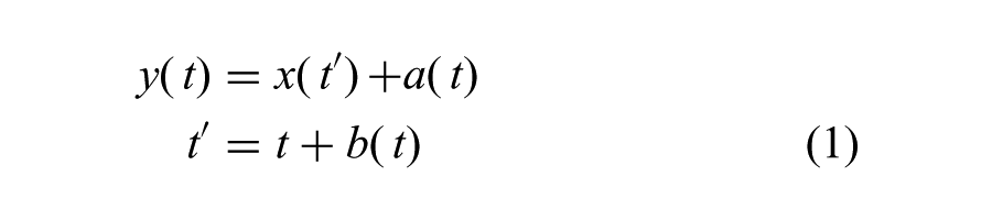
where x(t) is the first reference trajectory, y(t) is the second reference or output trajectory, a(t) is the set of time-dependent spatial shifts, b(t) is the set of time-dependent temporal shifts, t is time and t′ is the temporally shifted time variable, and where reference trajectory x(t) is being mapped onto y(t).
The correspondence problem is ill-posed, meaning that the set of spatial and temporal shifts is not unique. Therefore, a metric is often used to define a unique set of shifts.
Spatial-only metrics, which constitute the majority of “distance” metrics, are insufficient when data includes spatial and temporal relationships. Spatiotemporal-Isomap (ST-Isomap) is a common algorithm that takes advantage of STC in data to reduce dimensionality. However, the geodesic distance-based algorithm at the core of ST-Isomap was not selected as the candidate metric due to manual tuning of thresholds and operator input required to cleanly establish correspondence (Jenkins and Mataric, 2004). Another critical requirement for a metric is nonlinearity, since human motion data is nonlinear.
Our algorithm begins with the assumption that an input exemplar motion exists, for which human-like variants should be generated. To emulate the local coupling exhibited in human DOFs (e.g. ball-and-socket joints, muscular interdependence) on an anthropomorphic robot, which typically has serial DOFs, we optimize torque trajectories from the original motion according to the metric (based on parent and children DOFs, in the hierarchical anthropomorphic chain)
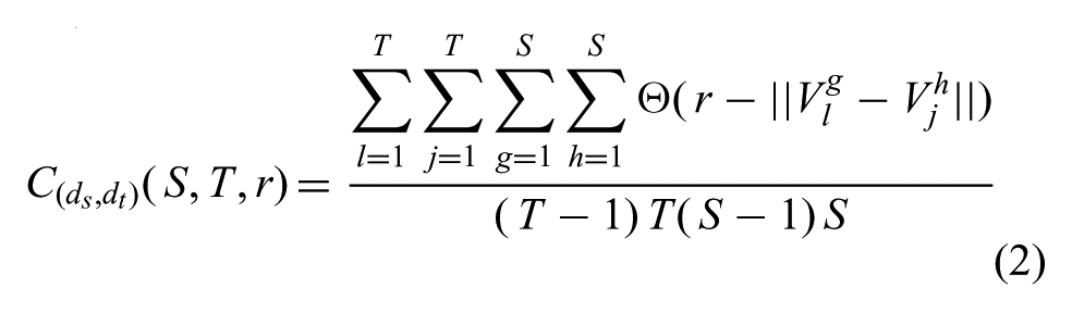
Before continuing, it might be helpful to provide some insight into the metric
where Θ(…) is the Heaviside step function,
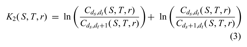
The K2 metric presented in Equation (3) constrains the amount of trajectory modulation in three parameters: r, S, and T. Here r can be thought of as a resolution or similarity threshold. Every spatial or temporal pair below this threshold would be considered equivalent and everything above it, non-equivalent and subject to modulation. We empirically determined a 0.1 N.m. threshold for r on the Simon robot hardware.
Based upon the assumption of a predefined input motion, temporal extent, T, varies based on the sequence length for a given motion. And, to emulate the local coupling exhibited in human DOFs on an anthropomorphic robot, the spatial parameter, S, is set at a value that optimizes only based upon parent and children DOFs, in the hierarchical anthropomorphic chain.
When modulating trajectories, the optimization begins at the “root” DOF (typically a rotationally motionless DOF, such as the pelvis), and it extends outward toward the fingertips. For Simon, this “root” DOF represents the rigid mount to the base. In other robots, the DOF nearest to the center-of-gravity is a logical place to begin the optimization, which can extend outward along each separate DOF chain. Any optimization that accepts a cost function can be used (e.g. optimal control, dynamic time warping), and the metric presented in Equation (3) would be substituted for the cost function in the problem definition.
4.2. Variance optimization
Once the process of inducing coupling between DOFs that are locally proximal on the hierarchy is complete, the output trajectory of the human-like optimization is used as the reference trajectory for a second optimization to add variance and satisfy constraints. The objective of this second optimization is to produce human-like variants without corrupting the original motion intent. The second optimization yields a biased torque that optimally preserves the characteristics of the input motion encoded in the cost function and any joint-space constraints. This biased torque is projected to the null space of Cartesian constraints to ensure that they are preserved. The resultant torque stochastically produces motion that is visually different from the input while maintaining constraints.
The core of our algorithm computes a time-varying multivariate Gaussian that has shaped covariance matrices,
Variation for an input motion is generated online by applying the following operations at each time step, which are explained in detail in subsequent sections. As closely as possible, we maintain the variable conventions for optimal control, so that notation is familiar from control theory.
Shape the torque covariance matrix for a Gaussian and draw a random sample:
Preserve joint-space constraints by appropriately defining two weight matrices: Qt and Rt, which scale the relative importance of the state and control terms, respectively, in the optimization.
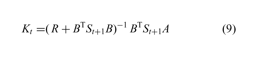
Compute the corresponding control force via the feedback control policy: Δut = −KtΔxt
Project the control force to enforce Cartesian constraints:
Apply the input motion and projected torque,
4.2.1. Shaping torque noise
Since the human-like optimization performs correspondence on torque trajectories, forward dynamics is used to compute the time-varying set of joint angles that comprise the motion. For the second optimization, the time-varying sequence of joint angles, qt, which were formed from the motion output from the human-like optimization are constructed into a reference state trajectory,
The goal of the variance optimization is to minimize the state and control deviation from the reference trajectory, subject to discrete-time dynamic equations
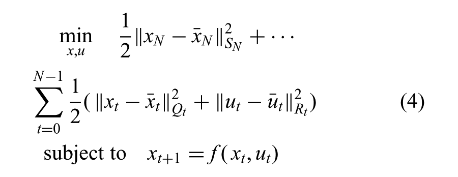
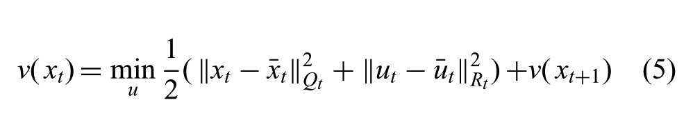
For an optimal control problem (Equation (4)), it is convenient to define an optimal value function, v(xt), which measures the minimal total cost of the trajectory from state, xt. Evaluation of the optimal value function defines the optimal action at each state. It can be written recursively, using the shorthand notation,
Our key insight is that the shape of this value function reveals information about the tolerance of the control policy to perturbations. With this, we can choose a perturbation that causes minimal disruption to the motion intent while inducing visible variation to the reference motion.
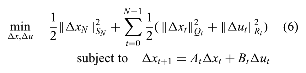
Both human and robot motion are nonlinear, and the optimal value function is usually very difficult to solve for a nonlinear problem. We approximate the full nonlinear dynamic tracking problem with linear quadratic regulator (LQR), which has a linear dynamic equation and a quadratic cost function. From a full optimal control problem, we linearize the dynamic equation around the reference trajectory and substitute the variables with the deviation from the reference, Δx and Δu:
where
Here SN, Qt, and Rt are positive semidefinite matrices that indicate the time-varying weights between different objective terms. We will discuss how these terms are computed to satisfy joint-space constraints later.
The primary reason to approximate our problem with a time-varying LQR formulation is that the optimal value function can be represented in quadratic form with time-varying Hessians:
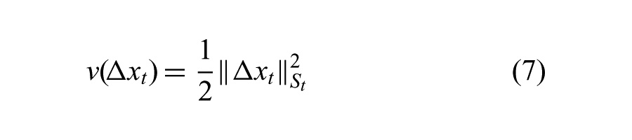
where the Hessian matrix, St, is a symmetric matrix.
The result of linearizing about the reference trajectory is that at time step t, the optimal value function is a quadratic function centered at the minimal point
We induce more noise in the dimensions consistent with tracking the human-like input motion by shaping a zero-mean Gaussian with a time-varying covariance matrix defined as the inverse of the Hessian,
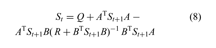
which exploits backward recursive relations starting from the weight matrix at the last time step, SN. We omit the subscript t on A, B, Q, and R for clarity (a detailed derivation is given by Lewis and Syrmos (1995)).
Solving this optimization defines how to shape the covariance matrices for all time so that variance can be added in dimensions consistent with the input motion, which in our case is the output of the human-like optimization step. But, we have not yet described how to create variance from the human-like input motion using these shaped covariance matrices.
4.2.2. Preserving joint-space constraints
Before we can solve the variance optimization, it is necessary to define the cost matrices in the optimization (i.e. SN, Qt, and Rt) appropriately so that joint-space constraints are preserved. The cost matrices define how closely the optimization output matches values of joint positions, velocities, or control torques. Since the weight matrices are time-varying, joint-space constraints are also time-varying. High weights at a specific time will generate variants that are biased toward preservation of that specific value at the appropriate time in all variants.
The cost weight matrices, SN, Qt Rt, can be selected manually based on prior knowledge of the input motion and control. Intuitively, when a joint or actuator is unimportant we assign a small value to the corresponding diagonal entry in these matrices. Likewise, when two joints are moving in synchrony, we give them similar weights.
We use Qt to denote the weight matrix for the state (i.e. joint position and velocity). Thus, to preserve joint-space constraints, the respective of weights of the desired DOFs in the Qt matrix are increased so there is a very high cost of deviation from the original trajectory. Similarly, Rt is the weight matrix for joint torques. To preserve the control from the input motion, high weights for the desired DOFs at the specific time instants will preserve this control torque in all of the output variants at the respective time instants. Joint-space constraints do not need to be specified outside of the time ranges for which they need to be satisfied to ensure they are met at the desired times. Since the optimal control problem is solved backward and sequentially, the formulation takes care of minimizing variance around temporally-local constraints so that motion remains smooth and human-like in all output variants.
In theory Q and R can vary over time, but in the absence of joint-space constraints, most practical controllers hold Q and R fixed to simplify the design process.
We propose a method to automatically determine the cost weights based on coordination in the reference trajectory. The weights for any DOFs constrained in joint-space should overwrite the values output from this automatic algorithm. We apply principal components analysis (PCA) on the reference motion
4.2.3. Computing the control force that corresponds to the shaped Gaussian sample
We are ready to solve the variance optimization and, thus, we describe how to create variations of the input motion using these shaped covariance matrices.
A random sample, Δxt, is drawn from the Gaussian
Occasionally, the Hessians of the optimal value function become singular. In this case, we apply singular value decomposition on the Hessian to obtain a set of orthogonal eigenvectors E and eigenvalues σ1 ⋯ σn (because St is always symmetric). For each eigenvector ei, we define a one-dimensional Gaussian with zero mean and a variance inversely proportional to the corresponding eigenvalue:
4.2.4. Preserving Cartesian constraints
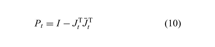
In addition to maintaining characteristics of the input motion, we also want variance that adheres to Cartesian constraints. At each iteration, we define a projection matrix Pt,
(where
We use the “dynamically consistent generalized inverse” (Sentis and Khatib, 2006)
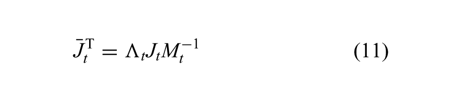
where Λ t and Mt are the current inertia matrix in Cartesian space and in joint space.
When we apply the projection matrix Pt to a torque vector, it removes the components in the space spanned by the columns of
4.2.5. Generating constrained variants
The final output after both optimizations is realized by applying the human-like motion torques,
4.3. Creating continuous motion
Since robots require the ability to move continuously, we describe how our algorithm can be used to continuously produce varied, human-like motion that respects constraints. We demonstrate that it is possible to transition to the next desired motion from a wide range of states. Furthermore, to make the transition reflect natural variance, we stochastically select the starting state of the next motion, called the transition-to pose, online so that it contains variance. We call our transition motions nondeterministic transitions because between the same two motions, different transitions are produced each time.
Once the next motion is selected, our algorithm determines a transition-to pose,
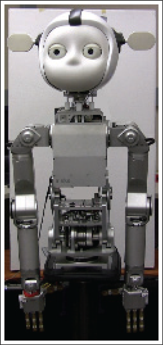
The robot platform used in this research is an upper-torso humanoid robot called Simon.
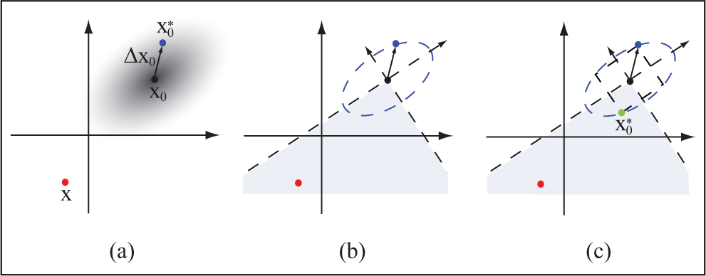
(a) Setting the transition-to pose to
To overcome this issue, we account for the current state, which is denoted as x in Figure 2, when selecting the transition-to pose,
After determining the transition-to pose, we use spline interpolation on the state and PID tracking to move the robot to this pose from the current pose. This works well because the transition-to pose is both consistent with the next motion and biased toward the current state.
5. Hypotheses
In the remainder of this paper, we evaluate the impact and effectiveness of different aspects of this pipeline for generating human-like motion. The respective hypotheses are divided up into categories based upon where the input motion is along the process of being transformed into human-like, constrained variants.
5.1. Human-like optimization
Our hypotheses are broken down into four distinct groups based upon topic. The first two hypotheses are based on our expectations for the human-like optimization.
H1: The human-like optimization increases motion recognition. Thus, motion that has been optimized with respect to STC will be easier for people to correctly identify intent (i.e. the task).
H2: Spatial and temporal correspondence separately are better metrics for human-likeness than composite STC.
When trajectories that were developed on one kinematic hierarchy (e.g. human) are applied to move another hierarchy (e.g. robot) that is kinematically or dynamically different (e.g. due to lack of DOF correspondence) motion trajectory data is lost. However, motion trajectory data can also be lost because the data is corrupted (e.g. insufficient sample rates in recording equipment). These are examples of using motion data in less-than-ideal conditions. The next three hypotheses are based upon the effects that we expect the human-like optimization to induce upon motion when used in less-than-ideal conditions. For rigor, we also include and test the ideal conditions. These hypotheses arise from our expectation that improving trajectory coordination from proximal motors offsets problems that arise due to DOF correspondence.
H3: The human-like optimization makes robot motion more human-like for imperfect (i.e. non-human-like) models. Thus, information lost due to DOF correspondence is regained by proximal DOF optimization with respect to spatiotemporal motor coordination.
H4: The human-like optimization has no effect when motion is projected onto a perfect model (i.e. when data-captured human and target model are sufficiently similar).
H5: The human-like optimization makes motion trajectories more human-like for imperfect data (i.e. when data loss exists). As more data is lost, the human-like optimization produces less optimal results.
5.2. Variance optimization
The next two hypotheses are relevant to the effect that the variance optimization has on the output of the human-like optimization. Since they are serial optimizations, ideally we want all our generated variants to be at least as human-like as the motion from which the variants are generated. Furthermore, the variance optimization should not corrupt the original intent of the motion (i.e. if the input is classified by observers as a wave, all variants should also be classified as a wave). We want to test both the quality of the variance optimization output, i.e. human-likeness, and the more fundamental property that our variance optimization produces variants (recognized and labeled same as the input motion).
H6: The variance optimization preserves human-likeness.
H7: The variance optimization preserves intent in the original motion.
5.3. Constraints
Our final three hypotheses test the effect of applied constraints on human-likeness and variance. The effects of constraints are tested in terms of both number of constraints and proximity of constraints to DOFs.
H8: As the number of applied constraints increases, motion becomes less coordinated and less human-like.
H9: As the number of applied constraints increases, variance decreases.
H10: Closer to location of application of a Cartesian constraint, the variance optimization produces less variance due to a smaller null space.
6. Experiment 1: Mimicking
The purpose of our first experiment is to quantitatively support that increasing STC of distributed actuators synthesizes motion that is more human-like. Since human motion exhibits spatial and temporal correspondence, robot motion that is more coordinated with respect to space and timing should be more human-like. Thus, we hypothesize that motor coordination as produced by SC and TC is a metric for human-like motion.
Testing this hypothesis requires a quantitative way to measure human-likeness. Distance measures between human and robot motion variables (e.g. torques, joint angles, joint velocities) in joint space cannot be used without retargeting (i.e. a domain change) due to the DOF correspondence problem. Thus, we designed an experiment based on mimicking.
In short, people are asked to mimic robot motions created by different motion synthesis techniques, and the technique that produced motions that humans were able to mimic the “best” (to be defined later) is deemed the technique that generates the most human-like motion. This experiment assumes that a human-like motion should be easier for people to mimic accurately, and awkward, less natural motions should be harder to mimic.
6.1. Experimental design
In this experiment human motion was measured with a Vicon motion capture system. We examined differences in people’s mimicking performance when they attempted to mimic the following three types of stimulus motion:
Original Human (OH): 20 motions captured from a male human, displayed on a virtual human model that precisely matches the marker data (i.e. no retargeting takes place).
Original Retargeted (OR): The OH motions were retargeted to the Simon hardware using a standard retargeting process (Gleicher, 1998).
Original Coordinated (OC): The OR motions were then coordinated using the human-like optimization.
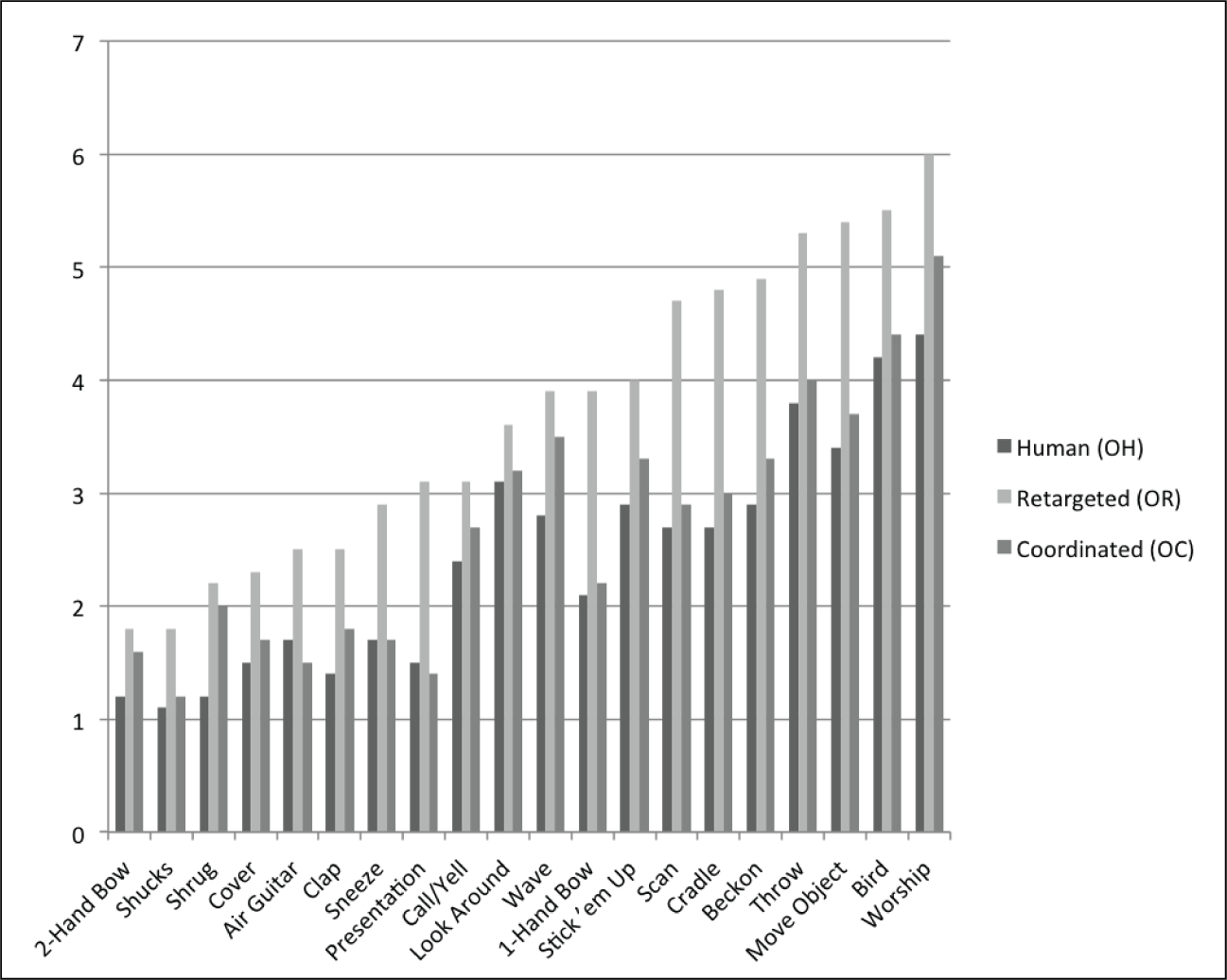
These three different “original” data sets were created before the experiment. The 20 motions used in the experiment included common social robot gestures both unconstrained and constrained, such as waving and object-moving, but also nonsense motions such as “air-guitar”. The full set of the motions used was: shrug, one-hand bow, two-hand bow, scan the distance, worship, presentation, air-guitar, shucks, bird, stick’em up, cradle, take cover, sneeze, clap, look around, wave, beckon, move object, throw, and call/yell. The latter six motions were constrained with objects for gesture directionality or manipulation, such as a box placed in a certain location to wave toward. When participants were asked to mimic such motions, these constraints were given to them to facilitate ability to mimic accurately. For all participants, the constraint locations and the standing position of the participant were identical. When constraints were given, they were given in all experimental conditions to avoid bias. The air-guitar motion was unconstrained because when humans perform an air-guitar motion, they do not have a guitar in their hands.
In the experiment, videos of motions were used for data integrity and motion repeatability. For example, if the robot hardware were used in the motion capture lab, the infrared light would reflect off the aluminum robot body and corrupt data. The original retargeted and original coordinated motion trajectories were videotaped on the Simon hardware from multiple angles for the study. Similarly, the original human motion was visualized on a simplified virtual human character (Figure 3) and also recorded from multiple angles. Each video of the recorded motion contained all recorded angles shown serially. There were 60 input (i.e. stimulus) videos total (20 motions for the 3 groups described above).
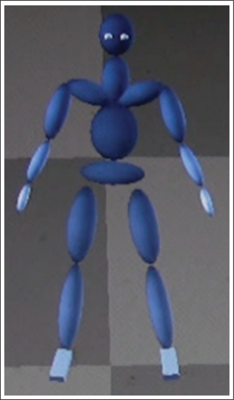
Virtual human model used in Experiment 1.
A total of 41 participants (17 women and 24 men), ranging in ages from 20 to 26, were recruited for the study. Each participant saw a set of 12 motions from the possible set of twenty that were randomly selected for each participant in such a way that each participant received four OH, four OR, and four OC motions each. This provided a set of 492 mimicked motions total (i.e. 164 motions from each of three groups, with 8–9 mimicked examples for each of 20 motions).
6.1.1. Part one: Motion capture data collection
Each participant was equipped with a motion capture suit and told to observe videos projected onto the wall in the motion capture lab. They were instructed to observe each motion as long as necessary (without moving) until they thought they could mimic it exactly. The video looped on the screen showing the motion from different view angles so participants could view each DOF with clarity. Unbeknownst to them, the number of views before mimicking (NVBM) was recorded as a measure for the study.
When the participant indicated they could mimic the motion exactly, the video was turned off and the motion capture equipment was turned on, and they performed one motion. Since there is a documented effect of practice on coordination (Lay et al., 2002), they were not allowed to move while watching and only their initial performance was captured. This process was repeated for the twelve motions. Prior to the 12 motions, each participant was allowed an initial motion for practice and to get familiar with the experimental procedure. Only when a participant was grossly off with respect to timing or some other anomaly occurred, were suggestions made about their performance before continuing. This happened with two participants, during their practice sessions, and those two participants’ non-practice data is included in the experimental results. No practice data from any participant is included in the experimental results.
After mimicking each motion, the participant was asked whether they recognized the motion, and if so, what name they would give it (e.g. wave, beckon). Participants did not select motion names from a list. After mimicking all 12 motions, the participant was told the original intent (i.e. name) for all 12 motions in their set. They were then asked to perform each motion unconstrained, as they would normally perform it. This data was recorded with the motion capture equipment, and in our analysis it is labeled the “participant unconstrained” (PU) set.
While the participants removed the motion capture suit, they were asked which motions were easiest and hardest to mimic; which motions were easiest and hardest to recognize; and which motion they thought that they had mimicked best (TMB). They were asked to give their reasoning behind all of these choices.
Thus, at the conclusion of part one of Experiment 1, the following data had been collected for each participant:
Motion capture data from 12 mimicked motions:
– 4 “mimicking human” (MH) motions;
– 4 “mimicking retargeted” (MR) motions;
– 4 “mimicking coordinated” (MC) motions.
Number of views before mimicking for each of the 12 motions above.
Recognition (yes/no) for each of the 12 motions.
For all recognizable motions, a name for that motion.
Motion capture data from 12 PU performances of the 12 motions above.
Participant’s selection of:
– easiest motion to mimic, and why;
– hardest motion to mimic, and why;
– easiest motion to recognize, and why;
– hardest motion to recognize, and why;
– which motion they thought that they mimicked the best, and why.
6.1.2. Part two: Video comparison
After finishing part one, participants watched pairs of videos for all 12 motions that they had just mimicked. Each participant watched the retargeted and coordinated versions (OR and OC) of the robot motion serially, but projected in different spatial locations on the screen to facilitate mental distinction. The order of the two versions was randomized. The videos were shown once each and the participants were asked if they perceived a difference. Single viewing was chosen because it leads to a stronger claim if difference can be noted after only one comparison viewing.
Then, the videos were allowed to loop serially and the participants were asked to watch the two videos and tell which motion in which video they thought looked “better” and which motion they thought looked more natural. The participants were also asked to give reasons for their choices. Unbeknownst to them, the number of views of each version before deciding “better” and more natural was also collected. The video order for all motions and motion pairs was randomized.
Thus, at the conclusion of part two of Experiment 1, the following data had been collected for each participant:
Recognized a difference between retargeted and coordinated motion after one viewing (yes/no); for each of 12 motions mimicked in part one (Section 6.1.1).
For motions where a difference was acknowledged:
– selection of retargeted or coordinated as “better”;
– selection of retargeted or coordinated as more natural.
Rationale for “better” and more natural selections.
Number of views before each of these decisions.
6.2. Results
6.2.1. H1: Human-like optimization increases recognition
The results presented in this section support Hypothesis 1, that our human-like optimization makes robot motion easier to recognize. The data in Figure 4 represents the percentage of participants who named a motion correctly, incorrectly, or who opted not to try to identify the motion (i.e. unrecognized). This data is accumulated over all 20 motions and sorted according to the three categories of stimulus video: OH, OR, and OC. Coordinated robot motion was correctly recognized 87.2% of the time, and was mistakenly named only 9.1% of the time. These are better results than either human or retargeted motion. In addition, coordinating motion led human observers to try to identify motions more frequently than human or retargeted motion (unrecognized = 3.7% for OC, compared with 8.5% for OH and 11% for OR). This data suggests that the human-like optimization (i.e coordinating motion trajectories) makes the motion more familiar or common.
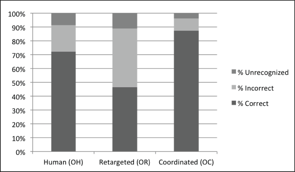
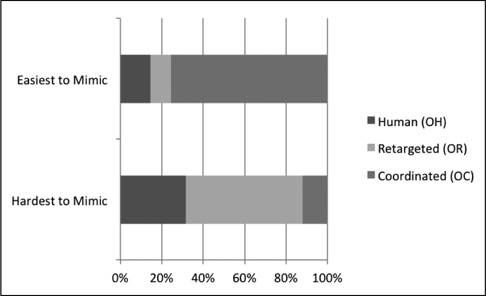
Percentage of motion recognized correctly, incorrectly, or not recognized by participants in Experiment 1, for each of the three categories of original data that they were asked to mimic. Spatiotemporal Coordinated motion is correctly recognized significantly more than simply retargeted motion, and at a rate similar to (but even higher than) the human motion.
On a motion-by-motion basis, the percentage correct was highest for 16 of 20 coordinated motions and lowest for 17 of 20 retargeted motions. In 17 of 20 motions percent incorrect was lowest for coordinated motions, and in a different set of 17 of 20 possible motions, the percentage incorrect was highest for retargeted motion. These numbers support the aggregate data presented in Figure 4 suggesting that naming accuracy, in general, is higher for coordinated motion, and lower for retargeted motion. Comparing only coordinated and retargeted motion, the percentage correct was highest for 19 of 20 possible motions, and in a different set of 19 of 20, percent incorrect was highest for retargeted motion. This data implies that relationships for recognition comparing retargeted and coordinated robot motion are maintained, in general, regardless of the particular motion performed. For reference, overall recognition of a particular motion (aggregate percentage) is a function of the motion performed. For example, waving was correctly recognized 91.7% of the all occurrences (OH, OR, and OC), whereas “flapping like a bird” was correctly recognized overall only 40.2% of the time.
The subjective data also supports the conclusion that coordinated motion is easier to recognize. When asked which of the 12 motions they mimicked was the easiest and hardest to recognize, coordinated was most often found easiest, and retargeted most often hardest. Figure 5 shows the percentage of participants that chose an OH, OR, or OC motion as easiest/hardest. A total of 75.3% of participants chose a coordinated motion as the easiest motion to recognize, and only 10.2% chose a coordinated motion as the hardest motion to recognize. A significant majority of participants (78.3%) selected a retargeted motion as the hardest motion to recognize.
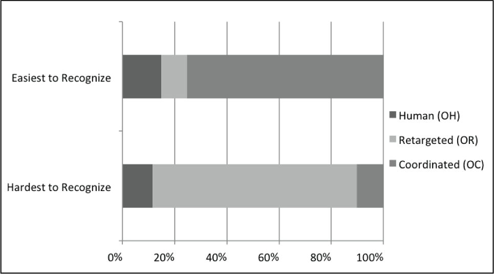
Percentage of responses selecting types of motions as easiest and hardest motion to recognize, for each of the three categories of original data that they were asked to mimic. Spatiotemporal coordinated motion is most often selected as easiest, and retargeted is most often selected as hardest.
When asked, participants claimed coordinated motion was easiest to recognize because it looked “better”, “more natural”, and was a “more complete” and “detailed” motion. And, retargeted motion was hardest because it looked “artificial” or “strange” to participants.
This notion of coordinated being “better” than retargeted is supported quantitatively by the second part of Experiment 1. In 98.98% of the trials, participants recognized a difference between retargeted and coordinated motion after only one viewing. When difference was noted, 56.1% claimed that coordinated motion looked more natural (27.1% chose retargeted), and 57.9% said that coordinated motion looked “better” (compared with 25.3% for retargeted). In the remaining 16.8%, participants (unsolicited) said that “better” or more natural depends on context, and therefore they abstained from making a selection. Participants who selected coordinated motion indicated they did so because it was a “more detailed” or “more complete” motion, closer to their “expectation” of human motion.
Statistical significance tests for the results in Figures 4 and 5 were not performed due to the nature of the data. Each number is an accumulation expressed as a percentage. The data is not forced choice; all participants were trying to correctly recognize the motion; some attempted and failed, and some did not attempt because they could not recognize the motion.
6.2.2. H2: SC and TC are better than STC
The following results from Experiment 1 support hypothesis H2, that optimizing based on composite STC rather than the individual components of SC and TC produces slightly worse results.
In Equation (3), the individual terms (spatial and temporal) on the right-hand side can be evaluated separately, rather than summing to form a composite STC. In our analysis, when the components were evaluated individually on a motion-by-motion basis, 20 of 20 retargeted motions exhibited statistical difference (p < 0.05) from the human mimicked data and 0 of 20 coordinated motions exhibited correspondence that is not statistically different (p < 0.05) than human data distribution. We will discuss these results in much more detail in Section 6.2.3. However, with the composite STC used as the metric, only 16 of 20 retargeted motions were statistically different than the original human performance (p < 0.05). Since the results were slightly less strong when combining the terms and using composite STC as the metric rather than analyzing SC and TC individually, we recommend that the SC and TC individual components be used independently as a metric for human-likeness.
6.2.3. H3: Makes motion human-like
Having completed the discussion on the general hypotheses for our human-like optimization, we have not yet completely proven that the optimization improves human-likeness in the presence of different models, agents, or data loss. Our robot, discussed in Section 3, represents a model or agent which is different kinematically and dynamically from a human. Thus, we can use Experiment 1 data to support our hypotheses regarding the effect of the human-like optimization on trajectories that are projected onto kinematic and dynamic hierarchies of DOFs (e.g. agents, models) that are different. The difference can be the result of DOF correspondence issues, and projection causes trajectory data loss. We call such trajectories: imperfect, which in the instance of Experiment 1, means non-human-like.
The data from Experiment 1 presented in this section supports hypothesis H3, that the human-like optimization (i.e. spatiotemporally coordinating motion) makes robot motion more human-like. In subsequent sections, hypothesis H3 will be refined (via hypotheses H4 and H5, Experiments 2 and 3, respectively) to be more general. These subsequent sections will show that for any model or agent that does not perfectly match the agent (i.e. the original human from which the original trajectory was motion captured or developed) and for large quantities of data loss, the human-like optimization makes any motion trajectory closer to human-like. This will be true in our case because the original trajectories were captured from a human.
Four sets of motion-capture data exist from Experiment 1, part one (Section 6.1.1.): MH, MR, MC, and PU motion. Analysis must occur on a motion-by-motion basis. Thus, for each of the 20 motions, there is a distribution of data that captures how well participants mimicked each motion. For each participant, we calculated the spatial and temporal correspondence according to Equation (3), which resolved each motion into two numbers, one for each term on the right-hand side of the equation. For each motion, eight or nine participants mimicked OH, OR, and OC. Three times more data exists for the unconstrained version because regardless which constrained version a participant mimicked, they were still asked to perform the motion unconstrained. Thus, for the analysis, we resolved MH, MR, MC, and PU into distributions for SC and TC across all participants. There are separate distributions for each of the 20 motions, yielding 4 × 2 × 20 unique distributions. The goal was to analyze each of the SC and TC results independently on a motion-by-motion basis, in order to draw conclusions about MH, MR, MC, and PU. We used analyses of variance (ANOVAs) to test the following hypotheses:
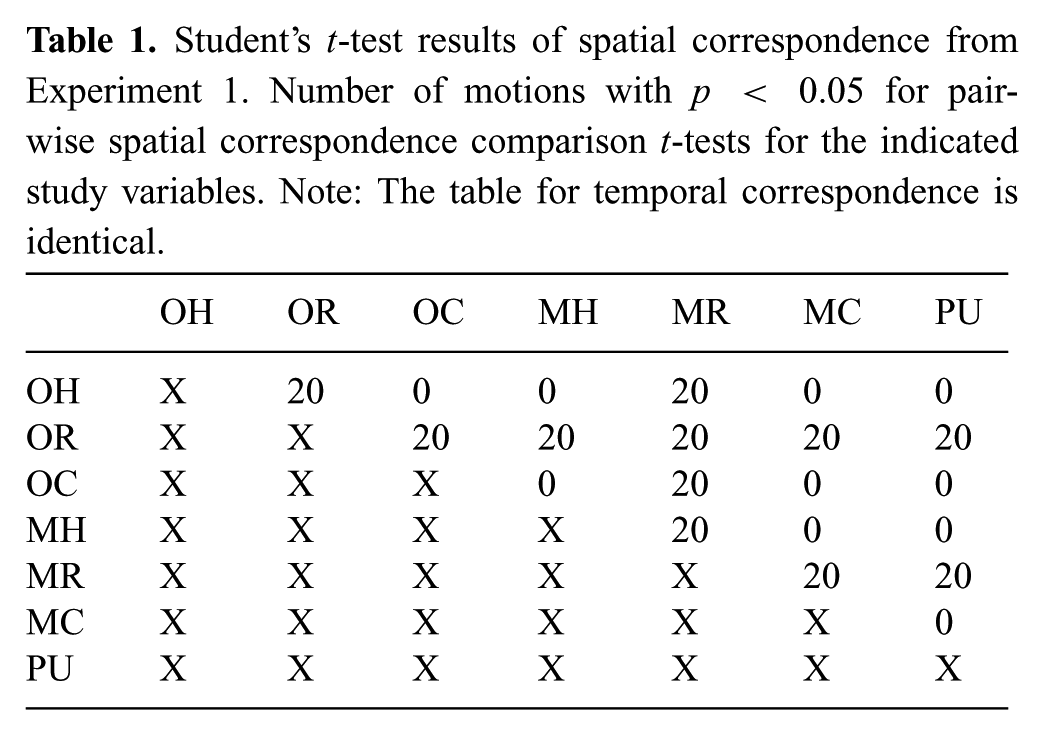
Since the above analysis isolated that retargeted motion was different from the other spatial and temporal correspondence distributions in mimicked motion, at this point, pairwise t-tests were performed to determine the difference between data sets on a motion-by-motion basis. Table 1 shows the number of motions for which there is a statically significant difference in spatial correspondence (the table for temporal correspondence is identical but not shown). For example, when participants mimicked retargeted motion, twenty motions were statistically different than the original retargeted performance. However, for the data when participants mimicked human or coordinated motion, the distributions failed to be different from their original performance for both SC and TC (H3.3). From this, we conclude that humans are not able to mimic retargeted motion as well as the coordinated or human motion.
Student’s t-test results of spatial correspondence from Experiment 1. Number of motions with p < 0.05 for pairwise spatial correspondence comparison t-tests for the indicated study variables. Note: The table for temporal correspondence is identical.
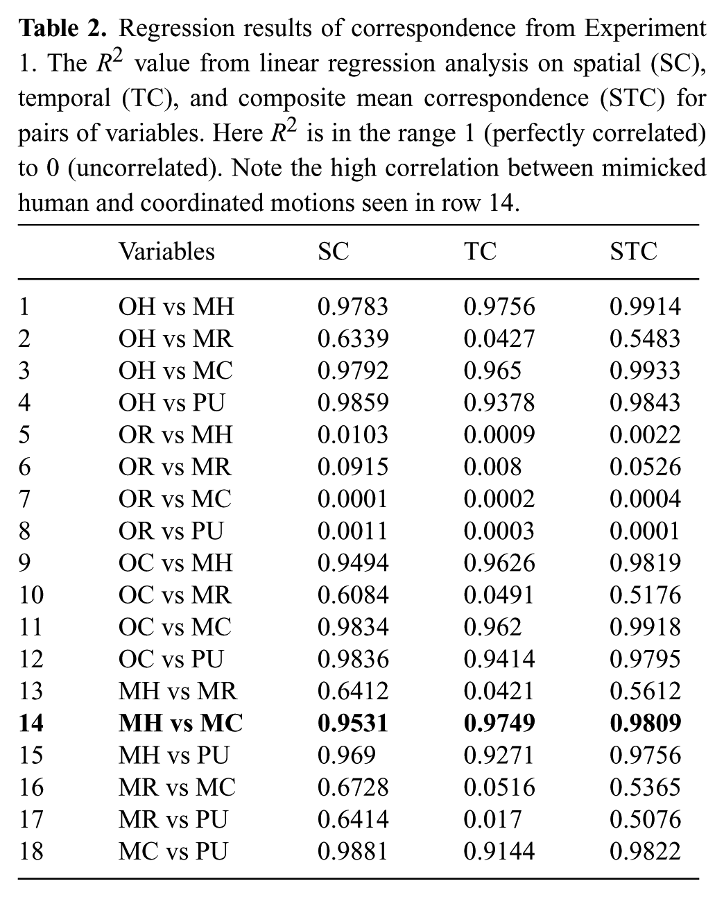
Since the above statistical tests do not allow us to conclude that the distributions were identical (H3.3), we performed a regression analysis of the data across all 20 motions to determine how correlated any two variables are in the study. For the purpose of this regression analysis the variables are either the mean or the standard deviation of SC, TC, or STC, for each of the distributions (OH, OR, OC, MH, MR, MC, and PU). However, the original data sets (OH, OR, and OC) are only one number (not a distribution) so they were not included in the standard deviation analysis. The intuition for this analysis is that if two variables are highly correlated with respect to both mean and variance, then it is further evidence that their distributions are similar. Specifically, results showing high correlation between the human and coordinated motions were expected, if Hypothesis 3 is to be supported.
The R2 values from the linear data fits, are shown in Tables 2 and 3. This data shows that participants mimicking coordinated and human motion were highly correlated (line 14 in Table 2 and line 2 in Table 3, shown in bold), whereas the data from when participants mimicked retargeted motion was less correlated to all other data including the original human performance (lines 2, 6, 10, 13, and 16 in Table 2). When two variables have high correlation in a linear data fit, it means that either variable would be a excellent linear predictor of the other variable in the pair. These higher correlations between human and coordinated motion are further evidence that coordinated motion is more human-like than retargeted motion.
Regression results of correspondence from Experiment 1. The R2 value from linear regression analysis on spatial (SC), temporal (TC), and composite mean correspondence (STC) for pairs of variables. Here R2 is in the range 1 (perfectly correlated) to 0 (uncorrelated). Note the high correlation between mimicked human and coordinated motions seen in row 14.
Regression results of standard deviation from Experiment 1. The R2 value from linear regression analysis on standard deviation of spatial, temporal and composite correspondence for pairs of study variables. Here R2 is in the range 1 (perfectly correlated) to 0 (uncorrelated). Variables not shown have a standard deviation of zero. Note the high correlation between mimicked human and coordinated motions seen in row 2.
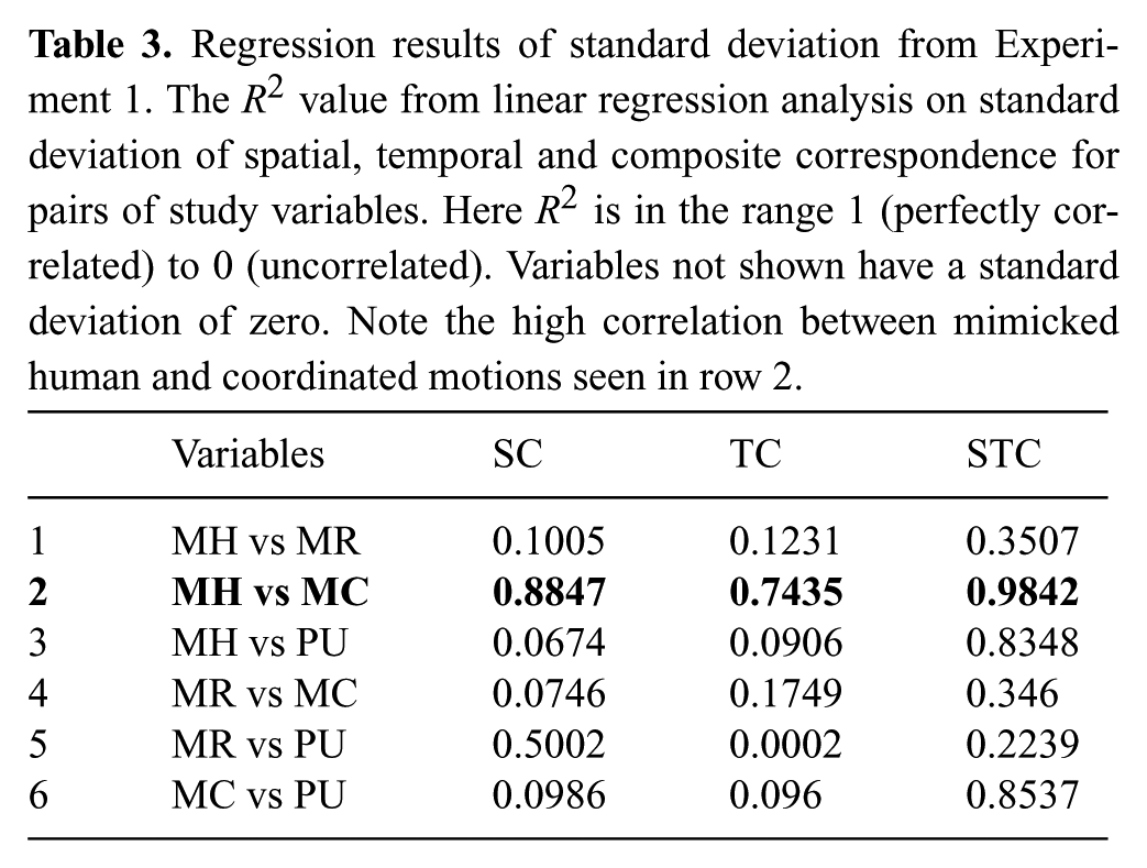
Furthermore, the standard deviation correlation on line 3 in Table 3 is low for the spatial and temporal components when regressing mimicked human and participant unconstrained data, which shows that mimicking does in fact constrain people’s motion. Variance increases for the PU distribution because motion is unconstrained and humans are free to perform the motion as they please. This validates our premise in Experiment 1 that mimicking performance is a better method by which to compare motion.
The data in Figure 6 shows the number of views before mimicking for each of the 20 motions, which also supports the claim that coordinated motion is more human-like. On average, humans viewed a retargeted motion more times before they are able to mimic (3.7 times) as compared with coordinated motion (2.7 times) or human motion (2.4 times). Pairwise t-tests between these distributions, on a motion-by-motion basis for NVBM, showed that 19 of 20 retargeted motions exhibited statistical significance (p < 0.05) when compared with human NVBM whereas only 3 of 20 coordinated motions NVBM were statically different (p < 0.05) from human NVBM. This suggests coordinated motion is more similar to human motion in terms of preparation for mimicking.
Average number of times participants watched each motion before deciding that they were prepared to mimic the motion. Retargeted versions of the motion always required the most views, whereas coordinated and human motion were usually more similar in number of views before mimicking.
Of the 12 mimicked motions, each participant was asked which motion was easiest and hardest to mimic. Of all participant responses, 75.6% of motions chosen as easiest were coordinated motions, and only 12.2% of participant responses chose a coordinated motion as hardest to mimic (Figure 7). In the assertion stated earlier, we claimed that a human would be able to more easily mimic something common and familiar to them. These results suggest that coordination adds this quality to robot motion, which improves not only ability to mimic, as presented earlier, but also perception of difficulty in mimicking (Figure 7).
Percentage of responses selecting types of motions as easiest and hardest motion to mimic. Coordinated is usually selected as easiest, and retargeted as hardest.
During questioning of participants in post-experiment interviews, we gained insight into people’s choices of easier and harder to mimic. Participants felt that human and coordinated motion were “more natural” or “more comfortable”. Participants also indicated that human and coordinated motion were easier to mimic because the motion was “more familiar”, “more common”, and “more distinctive”. In comparison, some people selected retargeted motion as being easier to mimic because fewer parts are moving in the motion. Others said retargeted motion is hardest to mimic because the motion felt “artificial” and “more unnatural”.
6.3. Summary of Experiment 1
The purpose of Experiment 1 was to support the general hypothesis that increasing STC of distributed actuators synthesizes more human-like motion. Our experimental design asked people to mimic motion that was either human motion, human motion retargeted to a humanoid robot, or additionally spatiotemporal coordinated motion. We find that people can more accurately recognize or infer the intent of STC motion, and they subjectively report this to be so. We show that SC and TC are more accurate metrics when used separately than in combination. Then find that based on such a metric, find that people are better able to mimic exactly a human motion or a coordinated motion, and are significantly worse at accurately mimicking retargeted motion. And this is also their subjective experience, most people found retargeted motion to be the hardest to mimic.
7. Experiment 2: Human motion
The purpose of Experiment 2 is to further quantitatively support that STC of distributed actuators is a good metric for human-like motion. Since human motion exhibits spatial and temporal correspondence, if SC and TC are good metrics for human motion, then optimizing human motion with respect to these metrics should not significantly change the spatial and temporal correspondence of human motion.
7.1. Experimental design
Experiment 2 was designed to test hypothesis H4, which is an extension to hypothesis H3. In Experiment 1, we tested retargeting human motion onto two different models: a human model and the Simon robot model. By doing so, we demonstrated that the human-like optimization recovers information lost when the model is imperfect. To state it precisely, an imperfect model is any model that is kinematically or dynamically different than the original agent who was motion captured. In Experiment 1, statistical difference of SC and TC groups for the retargeted robot motions showed that the retargeting process loses data when projecting onto an imperfect model (i.e. retargeting the human motion to the robot model). The advantage of the human-like optimization was that it was able to recover this lost data (e.g. we saw high correlation of the coordinated motion and human motion).
In Experiment 2, we focus on the human data to add evidence that SC and TC are good metrics for human motion. Hypothesis H4 extends H3 by demonstrating a complementary scenario: that less motion data is lost when models that are closer to ideal are used (i.e. the human-like optimization is unnecessary for projection onto ideal models).
We did not explain the details in Experiment 1, but the human model used for the motion captured data sets (i.e. the OH, MH, and PU) was actually 42 different human models (i.e. one for each participant and one for the human who performed the original, initial motions). The optimization for SC and TC in Equation (3) uses torque trajectories, and each human participant in Experiment 1 was physically different (e.g. mass, height, strength). In order to get accurate dynamic models for our human data, when Experiment 1 was performed, we collected basic anthropometric data from our participants: height, weight, gender, and age. Using the model scaling functionality of the Software for Interactive Musculoskeletal Modeling (SIMM) Tool 1 and the dynamic parameters we collected, we were able to produce accurate dynamic models of all humans, from which we collected motion capture data.
In Experiment 1, human participants were visualizing the OH data on the simplified human model shown in Figure 3. Although the SIMM tool provides trajectories for 86 DOFs, in the motion capture data, markers were not placed to sufficiently capture all 86 DOFs because we focus on body motion in this research. Thus, the number of DOFs in the human model was also simplified. DOFs in the eyes, thumbs, toes, ears, and face of the human model were removed since motion capture markers were not placed to capture sufficient motion in these areas when we collected data. Additional DOFs were removed in the human model in locations such as the legs, since the majority of these DOFs were not significantly animated in the 20 motions from Experiment 1 (i.e. they are upper-body motions). The final human model was comprised of 34 joints, concentrated in the neck, abdomen, and arms. When the motion capture data was retargeted to the human model, 45 markers were used as constraints to animate the 34 DOFs.
After each model was scaled for dynamic parameters unique to each participant (thereby creating 42 human models), the human motion capture data was retargeted to these 34-DOF simplified human models optimally. From this optimal retargeting, we had the original human and mimicked human (OH and MH) data sets. Since each participant in Experiment 1 mimicked 4 original human motions, we had distributions of mimicked human data formed from 8–9 human performances per motion. For Experiment 2, we combined these OH and MH data sets to create a data set that we call pre-optimization (pre-op), which consists of 9–10 similar human examples for each of 20 different motions.
To test H4, we optimized each of these 184 trajectories (4 MH motions per participant × 41 participants + 20 OH motions) according to the procedure in Section 4.1. This provided a comparison data set of 9–10 similar human examples for each of 20 different motions optimized according to the STC metric. This set is called post-optimization (post-op).
The SC and TC were evaluated for each of the trajectories in the pre-op and post-op data sets to create paired distributions of SC and TC for each motion. According to hypothesis H4, if SC and TC are good metrics for human-like motion, the optimization should not significantly affect them when the models used for retargeting and optimization are close to identical.
7.2. Results
For the initial analysis, on a motion-by-motion basis, 20 pre-op and 20 post-op distributions were combined to create 20 distributions (one for each motion). H4 states that SC and TC will not be affected by the human-like optimization when the data is not modified and the model accurately represents the agent who was motion captured. In other words, the SC and TC of the pre-op and post-op data come from the same distribution.
A total of 20 F-tests were performed, i.e. one for each combined motion distribution. The F values, for all 20 motions, were in the range 0.7–1.3 (spatial) and 0.8–1.4 (temporal), which were less than Fcrit = 4.4–4.5. Therefore, the data for all 20 motions was not statistically different before and after the optimization with respect to SC and TC. This data does not allow us to prove H4 definitively, but it is a first step toward understanding the performance of our human-like optimization. Since we believe that the metric is valid, we can increase confidence that the pre-op and post-op data belong to the same distribution with a regression analysis.
Assuming a normal distribution, high correlation between the pre-op and post-op distributions’ mean values and standard deviations would increase confidence in H4. Using the 20 independent data points (one for each motion), we formed linear regressions for the pre-op and post-op distributions’ mean values and standard deviations. After performing these four linear regressions, the correlation coefficient of the means was 0.9874 (SC) and 0.9657 (TC), and the standard deviations resulted in a correlation coefficient of 0.9791 (SC) and 0.9580 (TC). Ideally, the correlation coefficient of both of these regressions would be 1.0, which would indicate that they are identical distributions. The corresponding slopes of these two lines were 0.9954 (mean, SC), 0.9879 (mean, TC), 0.9481 (standard deviation, SC), and 0.9823 (standard deviation, TC). The ideal slope is 1.0, and these results show that the optimization did not significantly affect SC or TC of human-like motion when the models used for retargeting and optimization were identical.
7.3. Summary of Experiment 2
To summarize, in Experiment 2 we have strengthened the proof that STC is a good metric for human-like motion. In particular, we have shown that when the optimization is applied to motion that is already human-like (e.g. the OH and MH data sets from Experiment 1), the resulting motion is not significantly different from the original. Moreover, the SC and TC measures are highly correlated for both the pre-optimized and post-optimized versions of these motions.
In experiment 1 we learned that the human-like optimization procedure described in Section 4.1 can make retargeted motion more natural looking and easier for people to identify intent. Experiment 2 has additionally shown that applying our optimization to motion that is already human-like does not alter it significantly; that the human-likeness is left in tact.
8. Experiment 3: Downsampling human motion
This next experiment is designed to test H5, that our human-like motion optimization can work to recover information loss in situations with imperfect data.
In the last experiment, we provided evidence that the optimization does not significantly affect SC and TC for human-like motion when the model is identical for retargeting and optimization. With Experiment 3, we want to test the strength of the optimization in “retrieving” lost information and data. In other words, after Experiment 2 we knew that the optimization would function as expected under ideal conditions (i.e. ideal model and ideal data), but in Experiment 3 we wanted to test the metric to see whether it would function as expected when used in non-ideal conditions. One such non-ideal condition was discussed in Experiment 1: when the motion trajectory is used on an agent that was kinematically and dynamically different than a human (i.e. a robot). Experiment 3 tests the remaining non-ideal scenario.
The parameter K2 in Equation (3) from the human-like optimization is a metric from chaos theory that estimates the information lost as a function of time for a stochastic signal. In the human-like optimization, we used Kolmogorov-Sinai Entropy to estimate information difference between two deterministic signals (i.e. proximal DOF trajectories) and by correlating these two signals the robot motion became more human-like. Thus, in Experiment 3, we intentionally eliminate some information in the motion signal for an optimal model by downsampling the motion signal, and then we test how much of that information the optimization process is able to return for human motion. For example, this information loss could be due to motion trajectory transmission across a noisy channel or recording motion capture data at too low of a frequency.
8.1. Experimental design
For Experiment 3, we use the same human model and same two data sets from Experiment 2 (pre-op and post-op) for all 20 motions. We created eight new data sets, each of which represents the pre-op data set uniformly subsampled to remove information from the 184 trajectories. There were eight new data sets because the subsampling occurs at eight distinct rates: downsampling by rates in half integer intervals 2 from 1.5 to 5.0 (i.e. 1.5, 2.0, …, 5.0). These data sets are denoted by the label “pre-op” followed by the sampling rate (e.g. pre-op1.5 refers to the pre-op data set of trajectories with each trajectory subsampled by a rate of 1.5). For reference, the original pre-op data set from Experiment 2 represents pre-op1.0.
Then, we optimized each of the 1,472 trajectories (184 × 8) according to the procedure in Section 4.1 to create an additional eight new data sets for each of 20 motions. This provided paired comparison data sets of 9–10 similar human examples of each of 20 different motions for each of 8 unique sampling rates optimized according to the SC and TC metrics. These eight data sets are denoted by the label “post-op” followed by the sampling rate (e.g. post-op1.5 refers to the pre-op1.5 data set after optimization).
For each trajectory in these 16 new data sets (2,944 trajectories), SC and TC were evaluated. According to hypothesis H5, if SC and TC are good metrics for human-like motion, the optimization should compensate for SC and TC lost in the downsampling process when the models used for retargeting and optimization are identical. Also, H5 states that SC and TC for post-opN trajectories with subsampling rates closer to 5.0 will be less similar to the pre-op1.0 and post-op1.0 data sets for each motion.
8.2. Results
Since there are a large number of variables in the statistical significance tests (which result in many combinations of statistical tests), we will omit the details of the intermediate series of numerous tests that begin from the most broad hypothesis (i.e. that sampling rate has no effect on the pre-op1.0 trajectories; this means the optimized, downsampled, and original data (pre-op1.0, post-op1.0, pre-op1.5, post-op 1.5, …, pre−op5.0, post-op5.0) come from the same distribution). The intermediate set of tests led us to conclude the following:
Downsampled trajectories prior to optimization (pre-opN) were significantly different (p < 0.05) from pre-op1.0 and post-op1.0 for all sample rates N > 1.0, on a motion by motion basis for all 20 motions (with respect to both SC and TC). Thus, we conclude that degradation does cause a motion trajectory to lose spatial and temporal information.
Downsampled trajectories prior to optimization (pre-opN) were significantly different (p < 0.05) with respect to downsampled trajectories after optimization (post-opN) for all evaluated sample rates N > 1.0, on a motion by motion basis for all 20 motions (with respect to both SC and TC). We conclude that the human-like optimization significantly changed the spatial and temporal information of downsampled trajectories.
Downsampled trajectories prior to optimization (pre-opX) were significantly different (p < 0.05) from each other (pre-opY) on a motion by motion basis for all 20 motions (with respect to both SC and TC) for all sample rates where X ≠ Y. We conclude that downsampling at higher rates caused more spatial and temporal motion information to be lost.
The remainder of the pairwise t-tests are captured in Figure 8. In Figure 8 the data from Experiment 2 (i.e. pre-op1.0 and post-op1.0) is combined into a single distribution and compared against the SC and TC data from downsampled data sets after optimization (i.e. post-opN, where N > 1.0).
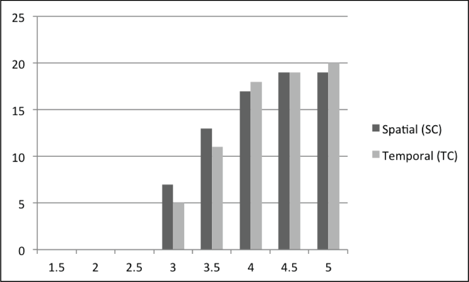
Number of motions with p < 0.05 for pairwise spatial and temporal correspondence comparison t-tests for the composite data set of pre-op and post-op (from Experiment 2) versus post-opN, where N = downsample rate. For downsample rates less than 4.0 the motion is often not significantly different than the non-downsampled version.
Numbers closer to 20 in Figure 8 indicate that more motions were unable to be recovered and restored with respect to SC or TC, as compared with the respective distributions without downsampling. Too much information was lost at higher sample rates (N ≥ 4.0), and the optimization was not able to compensate for the lost data, which provides evidence for the second half of H5. For lower values of downsampling rates, the optimization was able to perform well and recover lost information, but as downsampling rate increased less information was recoverable.
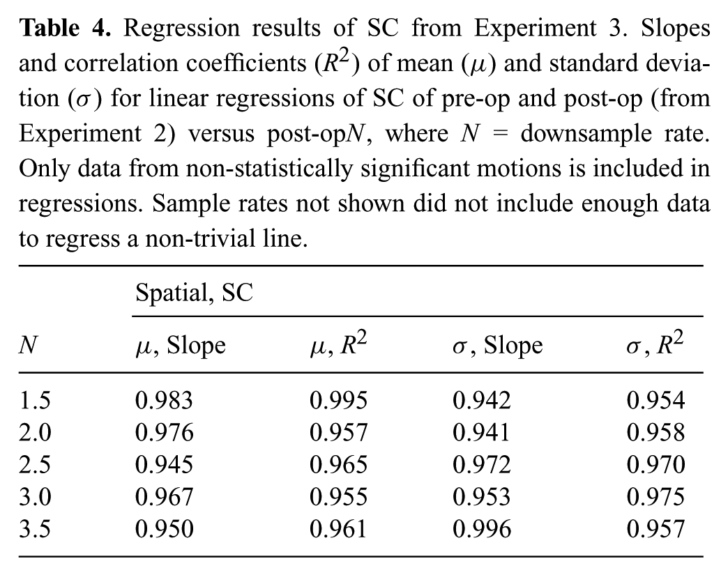
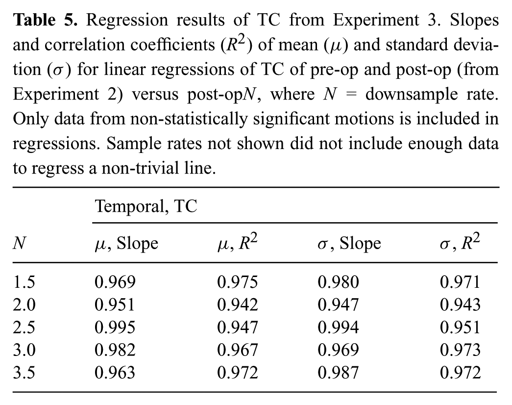
We would further like to say that for the sample rates N < 4.0 the resulting optimized motion is similar to the pre-op1.0 and post-op1.0 distributions. To do so we perform a linear regressions on the distribution means and standard deviations (pre-op1.0 and post-op1.0 versus post-opN). The slopes and correlation coefficients, as shown in Tables 4 and 5, indicate that for motion distributions that were not statistically different, the pre-op1.0, post-op1.0, and post-opN distributions are similar (slopes close to 1.0 with high correlation coefficient). This means that for downsampled trajectories where sufficient information content survives the downsampling process, after optimization, the distributions of SC and TC of these trajectories (on a motion by motion basis) appeared similar to the distributions where there is no information loss (pre-op and post-op from Experiment 2, without downsampling data).
Regression results of SC from Experiment 3. Slopes and correlation coefficients (R2) of mean (μ) and standard deviation (σ) for linear regressions of SC of pre-op and post-op (from Experiment 2) versus post-opN, where N = downsample rate. Only data from non-statistically significant motions is included in regressions. Sample rates not shown did not include enough data to regress a non-trivial line.
Regression results of TC from Experiment 3. Slopes and correlation coefficients (R2) of mean (μ) and standard deviation (σ) for linear regressions of TC of pre-op and post-op (from Experiment 2) versus post-opN, where N = downsample rate. Only data from non-statistically significant motions is included in regressions. Sample rates not shown did not include enough data to regress a non-trivial line.
8.3. Summary of Experiment 3
Experiment 3 is our final piece of evidence supporting that the human-like optimization that we have proposed is a good one. In Experiment 1 we showed it makes non-humanlike motion more human-like. In Experiment 2 we showed that is does not degrade already human-like motion. And in Experiment 3, we intentionally eliminate some information in the motion signal (by downsampling), and show that the optimization process is still able to recover that information to produce a human-like motion.
9. Experiment 4: Human-like variants
Experiments 1, 2, and 3 showed that human trajectories projected onto a robot kinematic hierarchy are more human-like if they are optimized with respect to STC. Now we would like create human-like variants for robot motion, which is why our variance optimization follows serially after the human-like optimization. For Experiment 4 we analyze the human-likeness after this variance optimization.
9.1. Experimental design
To demonstrate that the variance optimization maintains human-likeness when the optimized motion is already human-like, Experiment 4 proceeded in four steps. (1) In Experiments 1–3, we already supported that the input to the variance algorithm is human-like motion. (2) After the variance optimization, the SC and TC of the variants should not show statistical difference from the human-like optimization input motion SC and TC respective values. (3) Since step (2) does not allow us to make any claims about distribution equality between input and output motions for the variance optimization, we show high correlation between these distributions using a regression analysis. (4) Finally, to strengthen our quantitative data from step (3) we performed an experiment that is explained in the next section.
For step (4), the 20 motions from Experiment 1 that represent the original coordinated data set were used as inputs to the variance optimization. These are the SC and TC coordinated versions of the human motion executed on the robot hardware. The first 12 variants of each motion were generated, according to the procedure described in Section 4.2, and videos were made of these variants running on the robot hardware. Three different viewing angles were used to help participants see the motions clearly. These variants are labeled V1 to V12, and V0 represents the input motion to the variance optimization. Videos were used so that participants would be able to rewatch motions more easily.
Order of the twenty motions was randomized for each participant. The 13 videos (1 input and 12 variants) for the first randomly selected motion were shown to the participant in a random order. The participant was asked to select the most human-like motion from all thirteen. Participants were allowed to rewatch any videos in any order as many times as desired before making their selection. The experiment concluded when the most human-like version for all 20 motions was selected.
9.2. Results
The SC and TC of the variance optimization outputs (i.e. the motion variants) should not show statistical difference from the human-like motions’ (i.e. variance optimization inputs) SC and TC respective values. Thus, we compare the SC and TC distributions before and after the variance optimization. The original coordinated data set is only one data point per motion prior to the variance optimization (i.e. the variance optimization input, which is the original coordinated data from Experiment 1, is not a distribution for each motion), and neither SC nor TC can be averaged across motions. We are making comparisons of human-likeness on the robot hardware, and therefore we have a couple options for comparison data sets from Experiment 1 that will produce distributions that are representative for motions after the human-like optimization. The following are valid representative distributions after the human-like optimization because the analysis in Experiment 1 showed high correlation between these distributions (i.e. they were representative of human-like motion on the robot hardware).
OC (Original Coordinated): This is the OH data set from Experiment 1, optimally retargeted to the robot model (which became the original retargeted data set), and then processed through the human-like optimization. This is identical to the original coordinated data set from Experiment 1. One example per motion.
MHC (Mimicked Human Coordinated): This is the MH data set from Experiment 1, optimally retargeted to the robot model, and then processed through the human-like optimization. Eight or nine examples per motion.
MCC (Mimicked Coordinated Coordinated): This is the MC data set from Experiment 1, optimally retargeted to the robot model, and then processed through the human-like optimization. Eight or nine examples per motion.
PUC (Participant Unconstrained Coordinated): This is the PU data set from Experiment 1, optimally retargeted to the robot model, and then processed through the human-like optimization. There are 24–27 examples per motion.
The latter three options (MHC, MCC, and PUC) represent different sets of human participant data from Experiment 1 (i.e. the first two acronym characters), which undergo optimal retargeting and then the human-like optimization. Each of the 4 options (after the human-like optimization but before the variance optimization) had 12 variants generated per example per motion, to create a respective comparison data set distribution after the variance optimization.
We performed pairwise t-tests on each of these four data sets (OC, MHC, MCC, and PUC) compared against their respective data set after the variance optimization, and found that none of these tests showed statistical difference in the SC or TC dimension. This begins to support H6, that the variance algorithm does not alter human-likeness of the input motion. However, a regression analysis is required to provide conclusive support.
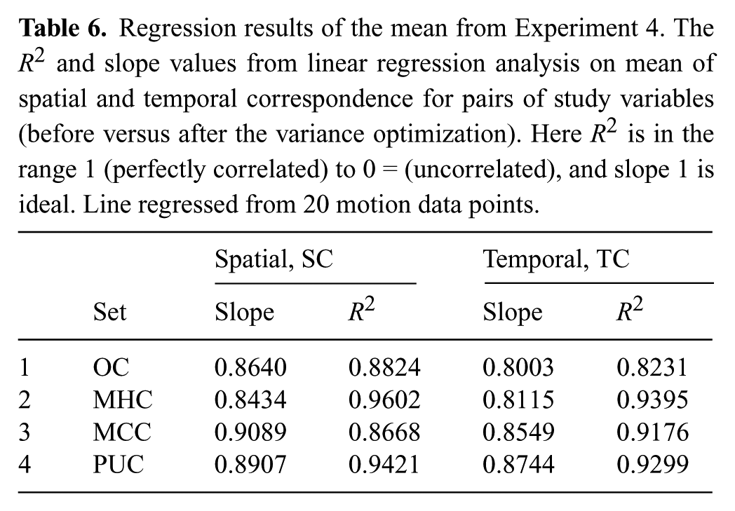
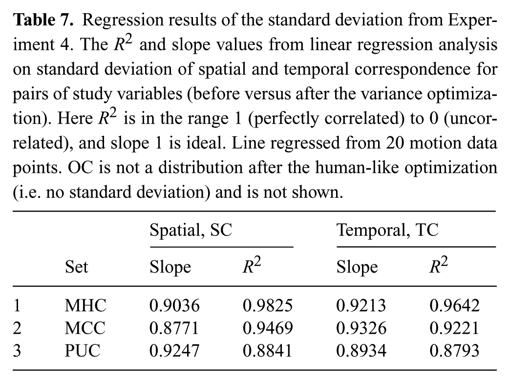
Tables 6 and 7 show that the distribution of spatial and temporal correspondence is fairly well maintained before and after variance optimization, regardless of the human-like motion data on the robot that is used. The high correlation numbers and slopes close to one provide insight that under the assumption of Normal distributions for this data, the variance optimization does not significantly change the distribution. These distributions represent the amount of SC and TC in the motions, and it is important to remember that SC and TC are not measures of amount of variance in motion.
Regression results of the mean from Experiment 4. The R2 and slope values from linear regression analysis on mean of spatial and temporal correspondence for pairs of study variables (before versus after the variance optimization). Here R2 is in the range 1 (perfectly correlated) to 0 = (uncorrelated), and slope 1 is ideal. Line regressed from 20 motion data points.
Regression results of the standard deviation from Experiment 4. The R2 and slope values from linear regression analysis on standard deviation of spatial and temporal correspondence for pairs of study variables (before versus after the variance optimization). Here R2 is in the range 1 (perfectly correlated) to 0 (uncorrelated), and slope 1 is ideal. Line regressed from 20 motion data points. OC is not a distribution after the human-like optimization (i.e. no standard deviation) and is not shown.
To strengthen our evidence that the variance optimization does not significantly affect human-likeness in motion data, we supplement our quantitative data with qualitative data. For step (4) (i.e. the experiment involving participants) only the original coordinated version after the human-like optimization was used because using additional data would result in the requirement of too many participants for all experimental conditions.
A total of 100 participants were recruited on the Georgia Institute of Technology campus (57 male, 43 female; ranging in age from 19–40). 100 participants yields a data resolution of 1% accuracy for results expressed as percentages.
In prior work, we established that torque space distance is a good indicator of degree of difference between two static poses (i.e. time instant states) in a motion (Gielniak and Thomaz, 2011). We now order the results from this experiment for all 12 variants according to increasing torque space distance from the input motion (i.e. the original coordinated version was used to create the variants) for all 20 motions. For this particular experiment, the torque-space distance metric allows us to order the variants by increasing variance from the original motion that created them.
Table 8 shows that when the first 12 variants are ordered by increasing torque space distance from input motion (i.e. the original coordinated motion), the percentage of participants choosing each variant as the most human-like of all 13 versions for a given motion is fairly uniform. Recall, that resolution on the data in Table 8 is 1%. From this data, we conclude that as the variants generated by the variance optimization look more different than the original motion, they maintain the human-like quality of that original motion.
Percentage of participants who selected a variant as the most human-like from the set of OC and the first 12 variants generated by the variance optimization. All data in the table are percentages. The variants are ordered by increasing torque-space distance from OC motion (increasingly different appearance). OC is the original coordinated motion. “Average” is the average percentage of participants over all variants. Note: The percentage resolution per motion is 1% due to number of participants.
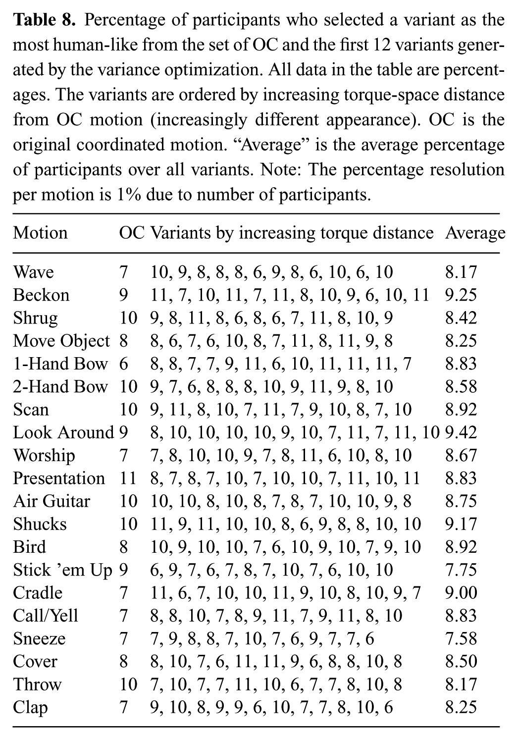
By contrasting Tables 8 and 9 the trend emerges. In Table 8 motions are not classified as more human-like as they become more different in physical appearance from the OC input motion. However, by ordering motions according to decreasing STC, which according to the human-like optimization yields more human-like motion, there is a very slight percent increase in responses of participants who labeled human-like motion in agreement with the STC trend (i.e. more human-like motion correlates to lower values of STC). Since the numbers in Table 9 represent variants and one input OC version per motion, the variant motions also obey the rule that human-like motion has lower STC. This data supports H6, that the variance optimization is not strongly affecting the human-likeness of the input motion.
Percent of participants who selected a variant as the most human-like from the set of original coordinated motions and the first 12 variants generated by the variance optimization. All variants and motions (including the input, original coordinated motions) have their respective percentages shown in the table and are ordered by decreasing STC (increasingly more human-like). Note: The percentage resolution per motion is 1% due to number of participants.
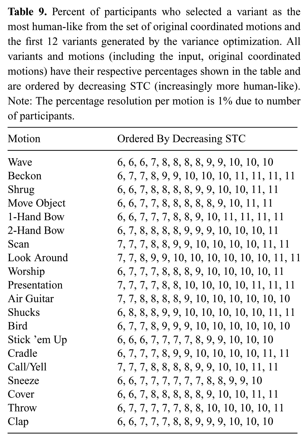
A total of 63.75% of the 240 generated variants (first 12 variants, 20 motions) had percent of participant values (selecting them as the most human-like of the 13 options for each motion) which were greater than or equal to the input original coordinated motion. In fact, 5 of the 20 motions only had zero or one variant that was selected by fewer participants than the input OC motion to be the most human-like version. This means that using an input motion that is human-like for the variance optimization will create variants that are subjectively deemed to be as human-like or more human-like as the input 63.75% of the time. Our variance optimization has a slight bias toward maintaining human-likeness.
10. Experiment 5: Variance optimization preserves intent
In the previous experiment we showed that the output of the variance optimization is still human-like, but we must also test that the intent of the original motion is preserved in the process of generating variants. According to H7, all variants should adhere to the definition of a true variant (i.e. they should be classified as the same motion type, gesture, or action as the original motion input to the variance optimization, from which the variants were created). In other words, when the robot moves using a variant, observers should perceive or label the robot intent to be the same as the intent they would perceive or label if the robot were moving using the input motion.
Experiment 5 demonstrates that the amount of variance produced by our algorithm is not so significant that it distorts variants to be labeled as gestures other than the original input motion.
10.1. Experimental design
In this experiment, 153 participants were asked label a single variant of five different motions. The five motions were: shrug (i.e. “I don’t know”), beckon, wave, bow, and point. Participants watched videos of motions executed on the hardware so that the experiment could proceed more quickly, be more repeatable, and be well controlled. Participants watched the videos through web-based code, sequentially, and the experiment was conducted over the internet. After a video stopped playing, the screen blanked and prompted the user for a label. The next motion video appeared after the label was entered.
The order of the 5 motions was randomized, and each participant saw either the original motion version or 1 of 12 variant versions created using our algorithm. For Experiment 5, the 12 selected variant versions for each motion were approximately uniform selections based on torque distance from each other, so that a larger portion of the space of visually different motions that can be produced by our algorithm could be covered in the analysis.
A total of 33 participants saw the original motion version for a particular motion, leaving 10 people who saw each variant version of that same motion. All orders and motions were randomized. No participant saw only original motion versions for all five motions.
10.2. Results
We use recognition as the metric for Experiment 5, to provide evidence that the variance optimization does not change motion intent. The task of the variance optimization is to produce a new version of the gesture that was given as the input motion. Thus, recognition (i.e. labeling of the variants with the same label as the original motion), was an appropriate metric to measure the success.
By comparing the bottom two rows in Table 10, we see that recognition rates are similarly high for the original motion and the variants. In four of five motions, percentage correct recognition is slightly higher for the variants than for the original motion. In addition, percentage correctly labeled is never more than 0.8% worse for the variants generated with our algorithm. Therefore, we conclude that the variance optimization does a good job of preserving task intent.
Labeling accuracy results from Experiment 5. Percentage correctly labeled (%) for 12 variants and the original motion of 5 different gestures (10 samples per variant, 33 samples for each original motion). Average for all motion variants as compared with the original motion shows that recognition does not decrease for generated variants (i.e. variants that are consistently labeled as the same motion type as the original motion).
11. Experiment 6: Highly constrained motion is less human-like
The final three experiments test the effect of constraints on either human-likeness or variance. From preceding experiments, we have demonstrated that the serial concatenation of the human-like and variance optimizations have successfully generated human-like variants of the original input motion. Since we claim that we can produce human-like, varied motion for robots, it is important to test how constraints influence our results, so that motion can be purposeful, human-like, and varied.
Experiment 6 is an analysis of human-likeness in the presence of increasing numbers of Cartesian constraints. According to hypothesis H8, as the number of constraints increases, SC and TC should decrease slightly for the human-like optimized motion after Cartesian constraints are applied. Hypothesis H8 is theorized as such because the dynamically consistent generalized inverse, which is essential in the projection that cancels constraint-affecting torques, does not account for human-likeness. Human-likeness should be affected very little when number of simultaneously-applied constraints is small. However, as the number of simultaneously applied constraints increases, the null space decreases, which means that there is less redundancy with which to move in a human-like manner. Thus, the resultant motion in the presence of high quantities of external constraints will be less human-like.
11.1. Experimental design
We designed Experiment 6 to test H8 and the interaction between the human-like optimization and external constraints. In previous experiments, participants were recruited to test whether spatially and temporally optimized motion appeared more human-like than other types of motions. SC and TC were presented as a metric for human-like motion to find a quantitative measure for humans’ subjective perception with respect to human-likeness in motion. Since hypotheses H1–H5 confirmed that the human-like optimization increases the human-likeness of motions, participants no longer need to be recruited to determine which motions are more human-like. Rather, Equation (3) can be used as a metric to tell which motions are more human-like (i.e. SC and TC closer to zero, more coordinated, are more human-like motion).
The intuition behind the design of this experiment is that if the benefits of lower SC and TC values are preserved in the presence of constraints, then motion with constraints remains more coordinated (and therefore, more human-like) than motion that excludes the human-like optimization.
We compare four types of motion.
Human Reference Condition (HRC): This is the baseline comparison data set for SC and TC; comprised of the original human motion and mimicked human motion data sets from Experiment 1. For this data set, SC and TC are evaluated on human models.
With Human-like Optimization (WHO): The HRC data set after the human-like optimization (without constraints). For this data set, SC and TC are evaluated on a robot model.
With Constraints Only (WCO): The HRC data set with constraints applied (without the human-like optimization). For this data set, SC and TC are evaluated on a robot model.
With Human-like Optimization and Constraints (WHC): The HRC data set after both the human-like optimization and applied constraints. For this data set, SC and TC are evaluated on a robot model.
The original human and mimicked human data sets were appropriate for the reference set because they represent human motion and were constrained by mimicking so the variance of SC and TC should be quite small. In Experiment 1, we showed that mimicking is an appropriate constraining method when motion comparisons must be made with respect to human-likeness.
To create the HRC data set, the motion capture trajectories from Experiment 1 for the original human and mimicked human (OH and MH) data were optimally projected onto human models as described in Experiment 2. Then the two halves of the right-hand side of Equation (3) were evaluated for trajectories for all 20 motions to create a distribution for SC and TC.
To create the remaining three data sets, the first step is to optimally project the OH and MH trajectories onto the Simon model. Then for the human-like set (WHO), we perform the human-like optimization, and then evaluate the two halves of the right-hand side of Equation (3) for SC and TC. The human-like and constraints (WHC) data set was created by taking the WHO data set and applying external constraints randomly before evaluating SC and TC. Finally, the constraints only (WCO) data set was created by optimally projecting the OH and MH data onto the Simon model, applying the same set of external constraints as for the WHC data set, and then evaluating SC and TC.
Specifically, we hypothesized that the data after the human-like optimization only (WHO) would have the lowest SC and TC values, followed by human-optimized and constrained data (WHC), and then the data with constraints only (WCO) because constraints are expected to decrease human-likeness on average and without the optimization to reduce STC, SC and TC are likely to be higher. If the results show this order, then we will have provided evidence in support of hypothesis H8. The results should also show that increasing constraints for the constrained data sets (i.e. WHC and WCO) should increase both SC and TC.
To strengthen the results, the number of simultaneously applied constraints varied from 1 to 5 for each of the 20 motions to help demonstrate that as number of constraints increases SC and TC decrease. For the purpose of data analysis, number of simultaneously applied constraints was assigned so that the same four motions only ever had one constraint applied, a different set of four only ever had two simultaneously-applied constraints, a different set of four only ever had three, etc.
H8 is independent of constraint type, and therefore, Cartesian position, orientation, look-at, or point-at were the types from which random selection was made. Each constraint was applied for a time duration of 5% of the total length of the trajectory. In cases where more than one constraint was simultaneously applied, all constraints were applied during the same time period and for the same duration. Constraint type, duration, number simultaneously applied, and time period of application were identical between the constrained data groups (WCO and WHC).
11.2. Results
On a motion-by-motion basis, treating all of the data (HRC, WHC, WCO, WHO) as if it comes from a single distribution, F-tests for both SC and TC for 20 of 20 motions yield p < 0.05, which indicates that at least 1 of these groups is statistically different from the rest of the data. Subsequent pairwise F-tests determined that 0 of 20 motions displayed statistical significance (p < 0.05) for HRC versus WHO (both SC and TC); 20 of 20 motions displayed statistical significance (p < 0.05) for HRC versus WCO (both SC and TC); 2 of 20 motions (SC) and 3 of 20 motions (TC) displayed statistical significance (p < 0.05) for HRC versus WHC. These results are consistent with Experiment 1 because WCO is a constrained form of retargeted human motion, similar to the retargeted motion (i.e. OR and MR) from that experiment, which also found statistical significance between human and retargeted human motion (i.e. the OH and MH versus OR and MR data sets in Experiment 1). There is no reason to believe that constraints will improve human-likeness. The five instances of constrained and human-optimized (WHC) motion that were statistically different all occurred for motions with five simultaneously applied constraints.
This begins to support H8, and can also be seen in Figures 9 and 10. As more constraints were added in both the constrained motion (WHC and WCO) groups, SC and TC increased, which means that motion became less coordinated. In the graphs each group shows all 20 motions ordered from most constrained at the top, and least constrained at the bottom. As stated in the previous paragraph all of the WCO motions were significantly less coordinated, which can be seen in their mean SC and TC values. In addition, with more constraints added to the motion, the SC and TC metrics began to exhibit noticeably larger differences between the WHC group and each of the reference condition and the human-like optimized only group. When number of constraints increased to 5 simultaneously applied, statistical difference was observed in all 5 instances. The overall values of SC and TC for the motion group that only had constraints increased as number of simultaneously applied constraints increased (from approximately 0.27 with 1 constraint up to 0.32 with 5 constraints for SC and TC).
Mean SC values for three data groups (WHO, WHC, WCO) as calculated by the respective parts of Equation (3). Motions are grouped according to number of simultaneously applied constraints (i.e. first four motions (cradle–scan) have five constraints, then clap–wave have four simultaneously applied constraints, etc.). HRC = OH + MH human data from Experiment 1; WHO = HRC projected to the robot model with SC and TC calculated after the human-like optimization; WHC = HRC projected onto the robot with both the human-like optimization and applied constraints; WCO = HRC on the robot model with only constraints applied.
This is the analogous graph to Figure 9, for mean TC values, which show similar trends as SC.
Furthermore, of the three data groups that were tested (WHO, WHC, and WCO), the set of motions that only underwent the human-like optimization (i.e. WHO) was the most coordinated motion of all three, as seen by the lowest SC and TC values in Figures 9 and 10. These values are also closest to the human reference condition (i.e. HRC) set values, which supports H8 that adding constraints begins to limit human-likeness.
12. Experiment 7: Highly constrained motion has less variance
Experiment 6 showed that as number of constraints increased, human-likeness decreased. However, we still need to study the effect of constraints on variance. Experiment 7 represents an analysis of variance in the presence of increasing the number of constraints. According to hypothesis H9, as the number of constraints increases, the variants should deviate less from their average value. No general claims can be made about the amount of variance in the variants relative to each other or relative to the motion input to the variance optimization because the degree to which these variants are similar to the input or to each other strongly depends on the selected constraints. Thus, as the number of constraints increases, deviation of the variants from each other or the input motion could increase or decrease because the appearance of the variants is a strong function of the selected constraints. Rather, hypothesis H9 is based upon a smaller null space as number of constraints increases. Since the variants are projected into the null space of the constraints in our algorithm, more constraint-disrupting torque is canceled, and therefore, less torque actuates the variants.
Variance should be affected very little when number of simultaneously applied constraints is small. Consider the simple example of one joint position constraint that lasts for the duration of the entire motion. Compared with the situation with zero constraints, all torque in that one DOF will be canceled and cumulative variance for the motion with one constraint will be less. When considering the extreme case where all DOFs are constrained by joint position for the duration of the entire motion, clearly variance become zero and motion ceases. Thus, the resultant motion in the presence of high quantities of constraints will be less varied.
12.1. Experimental design
We designed Experiment 7 to test H9 and the interaction between the variance optimization and constraints. However, since the case of joint position constraints is clear from the presented example, these particular constraints were excluded from the experiment. All other constraints were included: joint velocity, joint torque, point, orientation, point-at, and look-at.
In Experiment 7, three types of motion exist:
Robot Reference Condition (RRC): The 20 robot motions from Experiment 1, including one-handed (left or right arm) and two-handed gestures (symmetric).
With Variance Only (WVO): The RRC data set after the variance optimization (without constraints).
With Variance and Constraints (WVC): The WVO data set with applied constraints.
For the data set with constraints applied (i.e. WVC), a window of 5% of the motion length was chosen at random and up to 10 randomly selected constraints were applied during this window (i.e. each constraint was applied for a time duration of 5% of the total length of the trajectory). In cases where more than one constraint was applied simultaneously, all constraints were applied during the same time period and for the same duration. A total of 50 different variants were generated with 50 unique windows for each of 20 motions (i.e. 1,000 data points).
12.2. Results
Variance was calculated for each motion and the data is arranged in Figure 11 according to number of applied constraints. Figure 11 shows a distinct trend for constraints. As more constraints were added in both the WB group, average variance decreased, which is consistent with H9. There is a significant drop in variance above four constraints, and the constrained motions use only one-third of their joint angle ranges.
Mean variance for unconstrained (WVO) and constrained motion (WVC) ordered by number of constraints. The number following WVC indicates the number of constraints applied. Constraints were applied over a 5% trajectory length for all constrained data. Each row in the table is an average of 1,000 data points (50 variants of 20 different motions; 1 unique constraint window for each variant). Averages taken over all DOFs. Results are expressed as a percentage of total DOF range (limit to limit). For example, average variance of 50 would mean that the average DOF was utilizing 50% of its joint angle range for all variants.
The data in Figure 11 quantifies the average performance of the variance optimization. The ratio of WVO to RRC shows that the variance optimization on average produces motion that uses 3.5 times more of the joint angle ranges than in the original motions. This is consistent with the algorithm because we are adding biased torque noise in low cost dimensions, which, on average, results in an increased amount of motion in the variants. The ratio of 3.5 is also a good measure of “noticeablility” because it might be unintuitive to believe that injecting a small amount of torque noise would produce noticeably different variants. The 350% increase in use of joint angle ranges is a good indicator that variants will be noticeably different.
After 10 constraints are applied, nearly all motion is lost in the average DOF. According to the data in Figure 11, anything more than seven constraints applied causes very little use of joint angle ranges (i.e. little motion, little variance). Humanoid robots are very similar to humans, which cannot balance seven simultaneous tasks without sacrificing the lowest-priority tasks. Therefore, in a way, this is further evidence that the constrained variants are human-like.
13. Experiment 8: Constrained body parts exhibit less variance
In Experiments 6 and 7, we examined the effects of increasing the number of constraints. In our final experiment, we now evaluate variance as a function of proximity to the constraint. Although it might be intuitive that constrained body parts will move less, we provide Experiment 8 to demonstrate that constraints work as designed. The projection into the null-space to satisfy Cartesian constraints should affect the variance induced by the variance optimization more as proximity to the constraint increases. To support H10, Experiment 8 was designed to analyze variance in the presence of multiple constraints. Cartesian constraints on the robot’s body force the robot architecture to satisfy some geometry: point, line, or plane, which causes the constrained body parts to move less in Cartesian space. Observations such as these motivated hypothesis H10. Robot body parts that are connected in a series chain to a constrained body part will also exhibit less variance. These effects result from the null space because the null space is smaller closer to kinematically constrained body parts. We test the null space to provide quantitative support for hypothesis H10.
13.1. Experimental design
One point constraint and one orientation constraint were applied to the robot’s left hand for the entire duration of a shrug trajectory to constrain the hand so that a cup of water did not spill. Deviation in the left arm was then analyzed with respect to the original motion
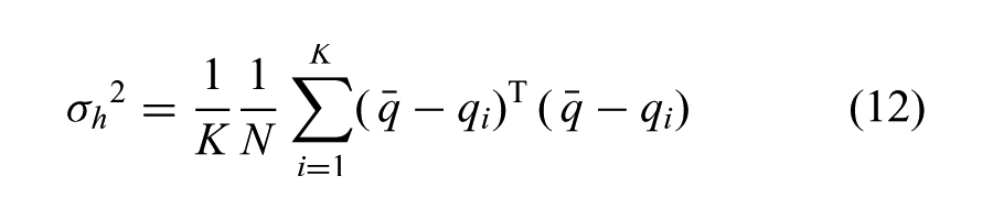
where
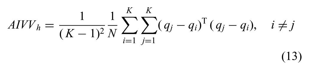
for two conditions: with and without constraints. Comparable numbers for constrained and unconstrained conditions on a per-DOF basis would support the null hypothesis that constraint projection does not adversely affect variance. This analysis was specifically performed on the arm closest to the constraint because part of hypothesis H10 suggests that variance decreases closer to the constrained location on the architecture.
13.2. Results
To measure variance in the presence of constraints, the variance of the left arm DOFs provided more insight into how constraints affect the motion because the left arm was closer to the constraint in the task. We first constrained the original motion, and then we used the original motion torques as the mean to compute the variance (Equation (12)). The results are shown in Table 11.
Deviation results from Experiment 8. Average variance (standard deviation) of joint angles for all left arm DOFs (in square degrees). Deviation from original motion and inter-variant variance (deviation between generated variants; labeled “between”) given for conditions of constrained and unconstrained motion. Averages taken using the first 12 motions generated by the variance algorithm for a shrug (“I don’t know”) gesture while constrained with the left hand holding a cup.
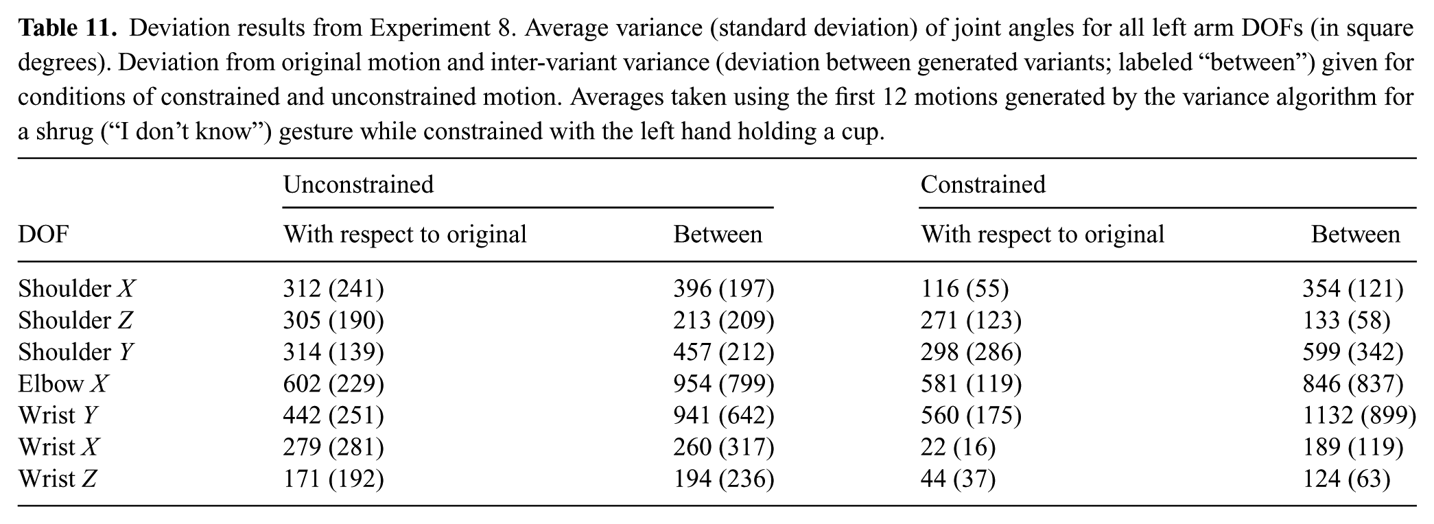
As expected, physical constraints reduce variance overall, as shown in Table 11. This was especially true closer to the actual constrained DOF, which for the cup constraint occurred in the wrist for the x and y DOFs. This effect was also evident in the calculations that reference the other variants. However, average variance between variants was still large for the left arm DOFs.
By comparing data for constrained and unconstrained, the trend was that constrained deviation was smaller when further from the wrist (i.e. point of constraint application). The constrained numbers approach unconstrained variance further from the wrist, which indicates the impact of constraints upon variance. From our analysis we concluded that the variance optimization also produces variance in constrained motion, provided that a null space for the constraints exists. H10 is supported since the data clearly indicates that variance is limited near the point of application of a constraint. As more constraints are added, less variance can be expected.
14. Discussion
We have presented an algorithm for generating human-like motion on robots in an autonomous way. Our underlying assumptions in this work are that: (a) the robot has controllable, independent actuators; (b) at least one input motion exists; and (c) the robot receives the constraints it must satisfy through sensors or a higher-level, decision-making algorithm.
Thus, given these assumptions, our algorithm is applicable to any robot that needs or wants to move in a more life-like manner. In this work, we have taken significant steps to show human-likeness, but it is likely that the algorithm will work for any biologically inspired robot that would have muscles if it were alive, because animal motion has also been shown to exhibit spatiotemporal coordination due to their musculature (Hayfron-Acquah et al., 2001).
The three components of our process are as follows.
Spatiotemporal coordination: We optimize motion with respect to STC, which emulates the coordinated effects of human joints that are connected by muscles.
Variance: We add variance to avoid repetitive motion by exploiting redundant and underutilized spaces of the input motion, which creates multiple motions from a single input. Possessing multiple versions of the same motion gives the robot the ability to choose a collision-free path when faced with obstacles.
Constraints: We maintain the robot’s ability to interact with its world by providing it the ability to satisfy constraints.
The extent of the work thus far has focused on validating these three components of our pipeline for generating human-like motion in a series of eight experiments that we have presented here.
14.1. Summary of findings
Experiments 1, 2, and 3 validated the first component of our algorithms, the human-like optimization of Spatiotemporal coordination. In Experiment 1 we learned that the human-like optimization can make retargeted motion more natural looking and easier for people to identify intent. Experiment 2 additionally showed that applying our optimization to motion that is already human-like does not alter it significantly; that the human-likeness is left intact. And Experiment 3 showed that even when we intentionally eliminate some information in the motion signal (by downsampling), the optimization process is still able to recover that information to produce a human-like motion. Thus, we conclude from this collection of experiments that increasing STC of distributed actuators synthesizes more human-like motion.
Next in the pipeline is the ability to produce multiple variants of a single input motion. Remember that the motivation for doing this is that humans rarely if ever repeat a motion exactly the same way twice, thus the ability to add variance in a human-like way is an important step in our process. In Experiment 4 we validated that the output of our variance optimization is still human-like. And in Experiment 5 we demonstrated the amount of variance produced by our algorithm and validated that it does not distort the input motion so much as to hinder people’s ability to recognize the motion’s intent.
The final piece in the pipeline is a practical one for robots that need to generate a particular motion in the face of environmental or task constraints (e.g. a target location/orientation of a particular joint, a look-at constraint during the motion, etc.). In Experiment 6 we showed that as more of these constraints are added the human-likeness of the resulting motion is decreased. In Experiments 7 and 8 we analyzed variance in the presence of increasing constraints, and at a joint level as a function of proximity to the constraint. Thus, as expected as the number of constraints are increased for a motion, then the ability for our algorithm to produce human-like varied motion decreases. But we found that in the presence of less than five simultaneous constraints our approach is successful in generating human-like motion.
14.2. Implications for human–robot interaction
Our future work will explore the benefits that human-like motion has on human–robot interaction. For example, we have shown that human-like motion produces improved motion clarity and better recognition for human partners, but what are the distinct benefits that both partners derive because humans are better able to tell what the robot is doing? Will collaboration progress more quickly? Will joint action be smoother with fewer errors? Will human enjoyment and satisfaction with the robot and the interaction improve? Will coordination between partners be more accurate and efficient? Will interactions achieve higher success rates when robot motion is more human-like? Will humans interact with robots longer or feel more engaged in interactions because the robot exhibits human-like motion? These and many other questions are the higher-level goals of our work with human-like motion. Demonstrations of these benefits and many others will become the motivation for others to equip their robots with our algorithm to autonomously generate human-like motion. Addressing these benefits will also enable others’ to decide where, when, and how exactly to use the algorithm that we have outlined herein.
We have shown that our algorithm produces robot motion that human partners can more easily identify due to the human-likeness imparted by our optimization. And given that this human-likeness in motion is preserved in the presence of variance and constraints, robots that collaborate with human partners will more clearly indicate their intent to their partners if our algorithm is used to synthesize robot motion.
This paper revolutionizes trajectory design for robots since databases of numerous examples of different motions and complex dynamic equations of motion are no longer required to generate variance. Although higher numbers of constraints will restrict variance and human-likeness in robot motion, one exemplar of each motion type (e.g. one wave, one shrug, one reach) is all that is required for the robot to perform an infinite number of motions similar to the exemplar. That exemplar trajectory can even be observed to avoid storage issues. Furthermore, we have shown that imperfect observation of such trajectories is sufficient to still create human-like robot motion because our human-like optimization can recover information lost in the trajectory.
The challenges in using this algorithm are few. The robot requires a torque trajectory, which means that if the given trajectory is not in torque-space, inverse dynamics might need to be performed on the given trajectory (which would require a model of the agent from which the exemplar trajectory was obtained). The algorithm does not exclude the use of human motion capture data for the exemplar trajectory, but use of such data requires a projection algorithm between the human and robot models to provide the input trajectory in a proper form.
We also contribute spatial and temporal correspondence as a metric for human-like motion for robots. The impact of this contribution is that a consistent baseline, which is independent of kinematics and dynamics, is presented for motion comparison. The independence of this metric means that any two agents that have DOFs can have motion compared regardless of domain (e.g. cartoon, puppet, robot, human, virtual character). Our metric is the first metric that can be used to either evaluate or synthesize human-like motion. The additional advantages of our metric are that it is objective, does not require dynamic simulations, and it is not observer- or heavily data-dependent.
Our experiments have also shown that to adequately compare human motion data objectively, it must be constrained. We have done so using mimicking, which reduces the variance of the range of motions humans can produce so that data is comparable between different humans. Constraining motion via mimicking also restricts the variance induced due to difference in kinematics and dynamics for a human population, which further facilitates scientific inquiry and data analysis.
15. Conclusion
We have presented an algorithm that produces human-like variants of an input motion. This algorithm is made functional for real-world tasks by including a projection that allows the robot to satisfy constraints such as looking at, grabbing, or pointing at objects. Similarly, the algorithm allows robots to synchronize to their partners, provided that human partners’ actions can be observed. Through a series of eight experiments, we have shown that human-like robot motion improves recognition accuracy of robot motions, so that social partners can more easily and accurately tell what the robot is doing. This increased clarity in motion can improve collaboration fluidity and minimize distractions due to awkward robot motion. Variance was added to the human-like motion so that human-likeness would be further improved and robot motion would be less repetitive.
Footnotes
Funding
This work was supported by an Office of Naval Research Young Investigator Grant (grant number N000140810842) and a National Science Foundation CAREER Grant (grant number IIS-1032254).