
Abstract
In this paper we propose a new path planning algorithm for coverage tasks in unknown environments that does not rely on recursive search optimization. Given a sensory function that captures the interesting locations in the environment and can be learned, the goal is to compute a set of closed paths that allows a single robot or a multi-robot system to sense/cover the environment according to this function. We present an online adaptive distributed controller, based on gradient descent of a Voronoi-based cost function, that generates these closed paths, which the robots can travel for any coverage task, such as environmental mapping or surveillance. The controller uses local information only, and drives the robots to simultaneously identify the regions of interest and shape their paths online to sense these regions. Lyapunov theory is used to show asymptotic convergence of the system based on a Voronoi-based coverage criterion. Simulated and experimental results, that support the proposed approach, are presented for the single-robot and multi-robot cases in known and unknown environments.
1. Introduction
Many applications require robots to perform a given task in an unknown, partially known and/or dynamic environment. Robots operating under such conditions are faced with the problem of deciding where to go to get the most relevant information for their current task. We are particularly interested in the case where robots have to continually monitor or sense regions of interest for a long period of time. One way to solve this task is for the robots to generate closed paths that allow them to sense regions of interest. We will refer to such paths as Interesting Closed Paths (IC paths). The robots could then travel these closed paths for long periods of time until the monitoring task is done.
When the environment is known, the IC path planning problem consists of computing closed paths that allow the robots to sense the regions of interest in an optimal way according to some metric. However, when the environment is unknown, the robots must also learn the structure of the environment by identifying which regions are interesting and which are not. Hence, IC paths correspond to paths where the most sensory information can be obtained by the robots. In both cases (known or unknown environment), the key insight is to use a continuous-time control law based on Voronoi coverage, inspired by Schwager et al. (2009) and Cortes et al. (2004). In the unknown environment case, a parameter adaptation law inspired by Schwager et al. (2009) is used to estimate the environment description, which feeds into the Voronoi coverage controller.
In short, the proposed controller works as follows. The robots move along their paths, marking the areas they observe as interesting or not. While feeding these observations into a adaptation law that estimates the environment description, the robots simultaneously modify their paths, based on these estimates, by changing the location of the paths’ waypoints in order to optimize a cost function related to the informativeness of the paths. By informative paths, we mean paths with which the robots are able to sense the regions of interest in the environment. By performing gradient descent on the cost function, the proposed controller attempts to place the paths’ waypoints at the centroids of their Voronoi partitions, while also making sure that waypoints within the same path are not too far from one another. The result of this process is a set of paths that enable the robots to sense the regions of interest in the environment and avoid non-interesting regions. An example of the results of our proposed controller can be seen in Figure 1. As will be shown in later sections, this controller can be implemented in a distributed way and works by using a simple control action.
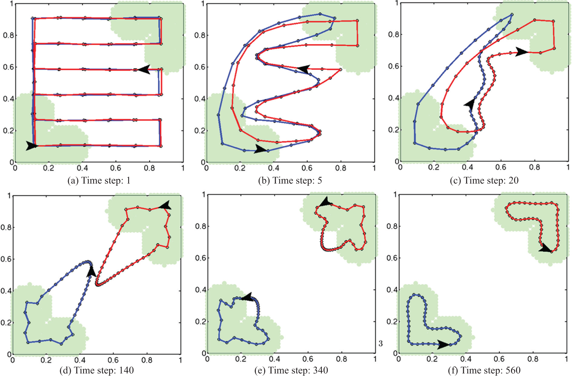
Simulated example of path shaping process for two robots with the IC path controller. The paths, shown as red and blue lines, connect the waypoints, shown as black circles. The blue path corresponds to robot 1, and the red path corresponds to robot 2. The robots’ positions are represented by the black arrow heads. The regions of interest in the environment, which the robots are tasked to cover, are represented by the light green regions. As time passes by, the paths are shaped such that the robots can cover the regions of interest. Each time step corresponds to a period of 0.01 seconds.
A wide range of applications require robots to move along IC paths in unknown environments in order to concentrate the robots’ resources in the regions of interest and avoid wasting them in non-interesting regions. For example, our algorithm could be used to monitor underwater life by allowing a team of robots to estimate the regions where underwater activity is high (e.g. coral reefs), and generate paths that enable the team to visit locations of high underwater activity. Our algorithm can also be useful for city surveillance tasks, where the robots need to monitor high-crime locations; robot vacuum cleaning tasks, where the robots need to visit locations that accumulate dust and avoid locations that remain clean; or estimation tasks, where the robots need to keep an updated mental model of the system’s state by visiting dynamic locations and avoiding visiting static locations.
The proposed IC path controller allows the user to have liberty of controlling the robots’ speed along the IC paths. Hence, depending on the application, different speed control policies can be used. To provide an example of such liberty, in this paper we combine the IC path controller with a speed control algorithm presented in Smith et al. (2011) in order to provide what is called persistent monitoring of an environment. To avoid confusion and distraction from our main contributions, we will refrain from elaborating on persistent monitoring for now, but will do so in a later section.
1.1. Contribution
In Soltero et al. (2012), we presented the single-robot case of the IC path controller in unknown environments, but, due to lack of space, important features about the algorithm were omitted. In this paper we not only elaborate on the results of the single-robot case, but also develop the theory for the multi-robot case in known and unknown environments, provide stability proofs using Lyapunov theory, show simulated as well as experimental results, and highlight some interesting features and limitations of the controller.
1.2. Relation to previous work
Most of the previous work in path planning focuses on reaching a goal while avoiding collision with obstacles (e.g. Piazzi et al., 2007) or on computing an optimal path according to some metric (e.g. Kyriakopoulos and Saridis, 1988; Qin et al., 2004). Other works have focused on probabilistic approaches to path planning (e.g. Kavraki et al., 1996). More relevant to this work is the prior work in adaptive path planning (e.g. Stentz, 1994; Cunningham and Roberts, 2001), which considers adapting the robot’s path to changes in the robot’s knowledge of the environment or changes in the system’s state.
The most relevant previous work is that of informative sensing, where the goal is to calculate paths that provide the most information for robots. The goal of Meliou et al. (2007) was to monitor a spatio-temporal phenomenon at a set of finite locations. The robot observes a subset of locations at any point in time and estimates other locations using a probability distribution, i.e. at each point in time they want to predict the values of all unobserved variables based on information collected up to that point. They solve the problem by planning closed paths that allow them to sense strategic locations according to some sub-modular metric. The work presented by Meliou et al. (2007) applies only to the single-robot case and is solved by search and iterative methods.
Binney et al. (2010) used previously obtained data to choose a path for an autonomous underwater vehicle (AUV) which gives the most additional information. This is done by optimizing over a sub-modular metric, which in their case is mutual information. Again, this solution is based on search and iterative optimization for a single robot, where the path is recursively divided in half and the next midpoint is searched and committed to before continuing to the next iteration.
Singh et al. (2009) used mutual information to obtain informative paths for a collection of robots, subject to constraints on the cost incurred by each robot (e.g. limited battery capacity). This problem is also solved by a search and iterative optimization. In addition, the currently published work is an offline algorithm, i.e. does not adapt the path with new data, and although it treats multiple robots, the algorithm is centralized. It plans the paths for each robot sequentially, each one taking into consideration all previous robots’ paths. Other variations on informative path planning include maintaining periodic connectivity in order for robots to share information and synchronize (Hollinger and Singh, 2010), and incorporating complex vehicle dynamics and sensor limitations (Levine et al., 2010).
All of the mentioned previous work in informative sensing and adaptive path planning, as with most in path planning in general, treats the path planning problem as a search and/or recursive problem, with running times that can be very high for large systems, and some of them only providing approximations of optimal solutions due to intractability of the problem. Also, many of them are centralized algorithms since path planning in a distributed way is a very difficult problem. In contrast to all of these previous works, we approach the path planning problem in a way that resembles the train of thought of artificial potential fields (Khatib, 1985) and behavioral dynamics (Large et al., 1999), where a dynamical systems approach is used in path planning and control. The idea behind these approaches is to generate a control law that governs robot behavior/motion based on behavioral dynamics and competition between constraints. One good feature of these kinds of solutions is that they can be much easier to implement in a decentralized way. In our case, we use a type of artificial potential field based on Voronoi partitions, but this potential field does not govern the robots’ behaviors. Rather it governs the behavior of waypoints that define the paths that the robots are following.
We approach the path planning problem as a continuous-time dynamical systems control problem. Furthermore, we focus most of our attention on the problem of path planning in unknown environments, where we use gradient-based adaptive control tools to control the location of waypoints that define robot paths. These gradient-based tools seek to locally optimize a Voronoi-based cost function related to the position of the waypoints. The Voronoi-based nature of our controller is partly inspired by the work of Graham and Cortes (2012), where a form of generalized Voronoi decomposition was used to design a sampling trajectory that minimized the uncertainty of an estimated random field. In our work, we also use a Voronoi decomposition as the basis of our algorithms, but the problem we are treating is different. In our work the field is not random (although unknown) and we are not concerned with minimizing predictive variance, but rather we focus on generating closed paths by optimizing the location of waypoints defining the paths, according to a Voronoi-based coverage criterion in an unknown environment. Because of this, our approach builds upon the work of Schwager et al. (2009) and Cortes et al. (2004), where a group of agents were coordinated to place themselves in static, locally optimal locations to sense an environment that is known (in the case of Cortes et al., 2004) or unknown (in the case of Schwager et al., 2009). In these works, Voronoi partitions were used to position the robots, while a parameter adaptation law allowed the agents to learn the environment model. We build upon these works by letting the waypoints in the robots’ paths define a Voronoi decomposition, and using a parameter adaptation law to learn which regions of the environment the robots should focus on sensing. This Voronoi-based adaptive controller provides a simple and distributed way of generating useful paths for the robots, with strong and simple stability guarantees.
The paper is structured as follows. In Section 2 we set up the problem, present locational optimization tools, and present a basis function parameterization of the environment. Section 3 introduces the IC path controller for the case where the environment in known to the robots. We then treat the case of robots operating in unknown environments in Section 4. After that, in Section 5, we show how controlling the speeds of the robots along the IC paths can be used to perform persistent monitoring tasks in unknown environments, and we provide results from an implementation with two quadrotors. Finally, we talk about some limitations and future work in Section 6 and present our conclusions in Section 7.
2. Problem formulation
We will use the convention of boldface variables to represent vectors. We assume we are given a number of robots whose tasks are to sense an environment while traveling along their individual closed paths, each consisting of a finite number of waypoints. The goal is for the robots to identify the regions within the environment that are of interest and compute paths that allow them to jointly sense these regions. A formal mathematical description of the problem follows.
Let there be N robots identified by r ∈ {1,…,N} operating in a convex, bounded area
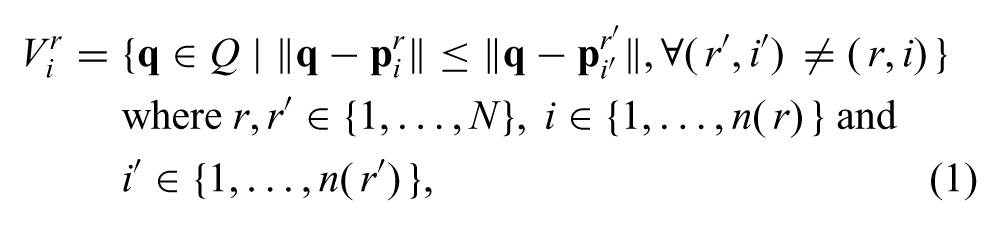
where ‖·‖ denotes the l2-norm. We assume that the robot is able to compute the Voronoi partitions based on the waypoint locations, as is common in the literature (Salapaka et al., 2003; Cortes et al., 2004; Schwager et al., 2009).
Since each path is closed, each waypoint
A sensory function, defined as a map
Remark 2.2. The interpretation of the sensory function φ(
2.1. Locational optimization
Building upon the work of Schwager et al. (2009) and Cortes et al. (2004), we now formulate a cost function
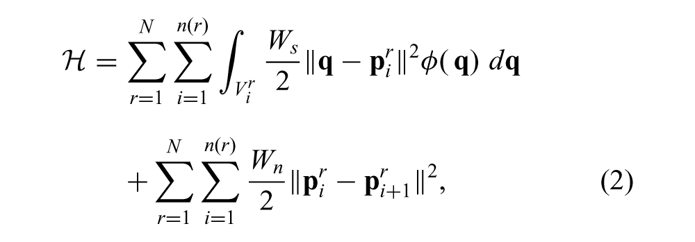
where
This cost function says two things: (1) paths that do not provide good/reliable sensing of the regions of interest are expensive; and (2) having neighboring waypoints (in the same path) be too far apart from each other is expensive. Consequently, by designing a controller that performs a gradient descent on this cost function, we introduce two primitives for the waypoint movements in each path. The first primitive drives the waypoints to move towards their Voronoi centroids in order to properly cover/sense the environment. The second primitive makes each waypoint pull its neighboring waypoints, which couples the waypoints in order to generate closed paths. The relative strength of the first and second primitive is specified by the user’s selection of the parameters Ws and Wn, respectively. A formal definition of IC paths follows.
Next we define three properties analogous to mass-moments of rigid bodies. The mass, first mass-moment, and centroid of the Voronoi partition
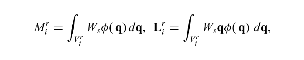

respectively. Also, let
From locational optimization (Drezner, 1995), and from differentiation under the integral sign for Voronoi partitions (Pimenta et al., 2008) we have
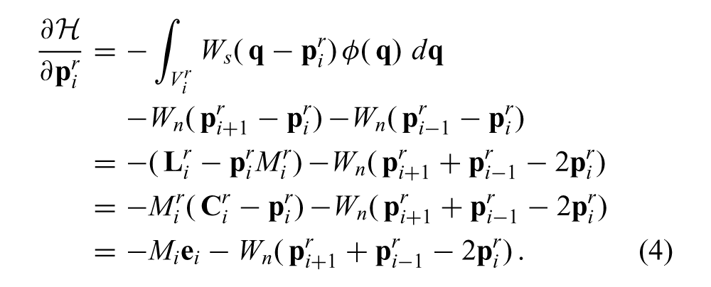
Assigning to each waypoint dynamics of the form

where
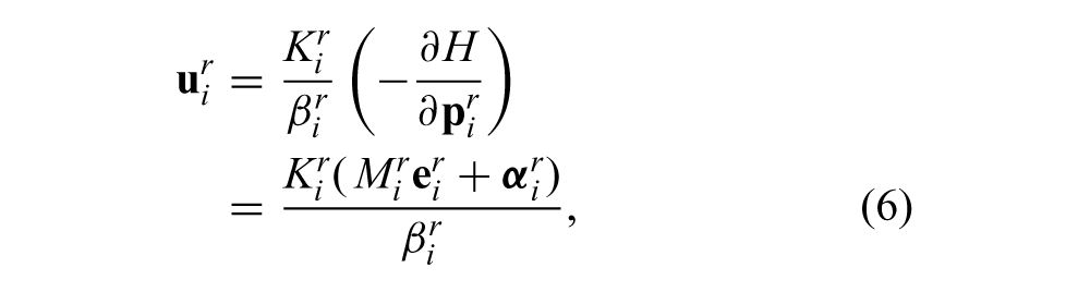
where

and
Remark 2.4. The term
2.2. Sensory function parameterization
We assume that the sensory function φ(
Assumption 2.5 (Matching condition). There exists
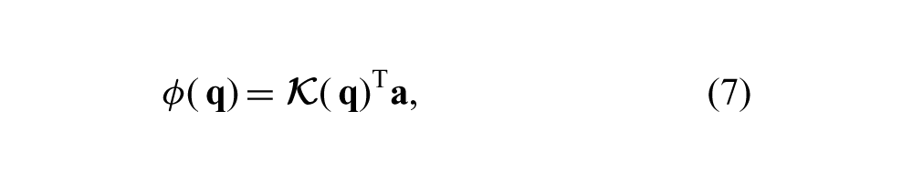
where the vector of basis functions
Such an assumption is common for adaptive controllers (Schwager et al., 2009).
3. IC path controllers for known environments
In this section we assume that the robots have knowledge of the sensory function φ(

Proof. We define a Lyapunov-like function based on the robots’ paths, and use Barbalat’s lemma (Ioannou and Sun, 1996) to prove asymptotic convergence of the system to a locally optimal equilibrium.
We define a Lyapunov-like function

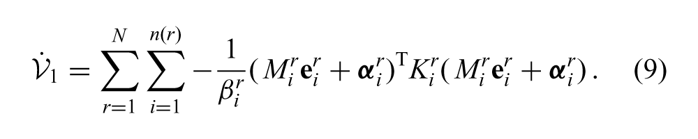
Taking the time derivative of
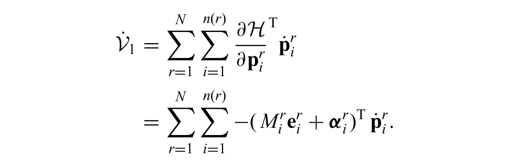
Substituting the dynamics specified by (5) and control law specified by (6), we obtain
Note that
Remark 3.2. Theorem 3.1 implies that the paths will reach a locally optimal configuration for sensing regions of interest, where the waypoints reach a stable balance between providing good sensing locations and being close to their neighbor waypoints. In addition, this balance can be tuned (short paths versus good coverage) by the proper selection of Wn and Ws.
3.1. Simulated results
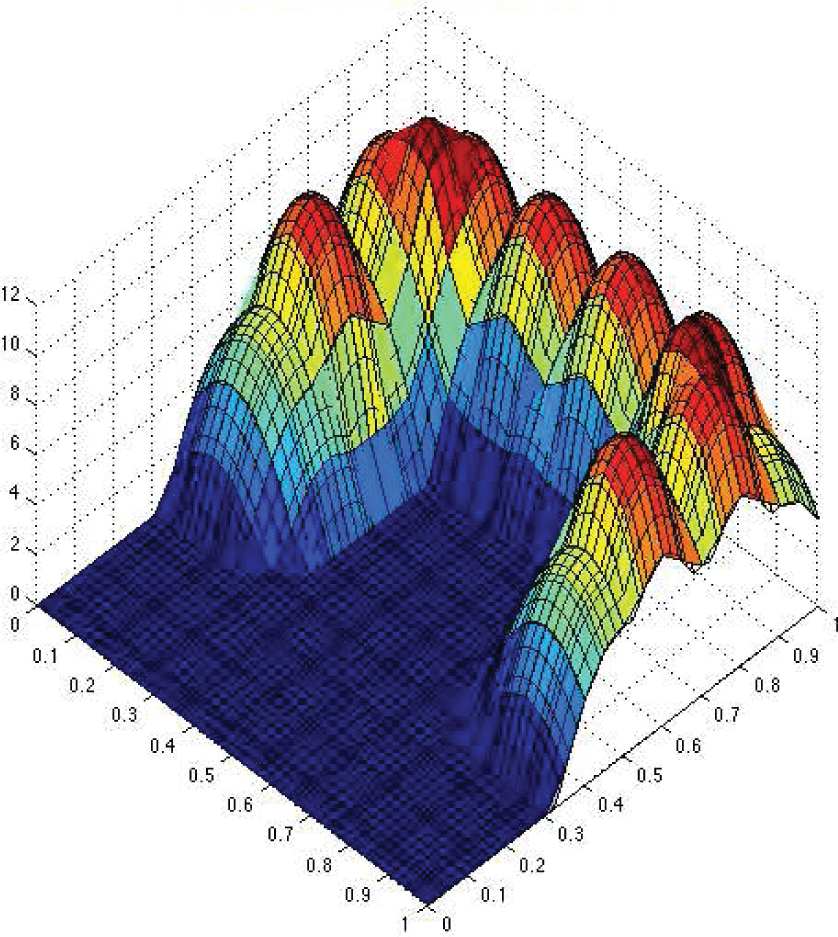
In this section we simulate the IC path controller for known environments for the simple case of a single robot, i.e. N = 1 and, therefore, r = 1. The simulation is performed in MATLAB. Here we present a case for n(r) = 40 waypoints. A fixed-time step numerical solver is used to integrate the equations of motion using a time step length of 0.01 seconds. The region Q is taken to be the unit square. The sensory function φ(
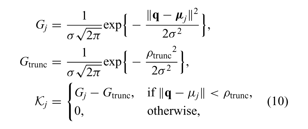
σ = 0.4 and ρtrunc = 0.2. The unit square is divided into an even 5 × 5 grid and each truncated Gaussian mean
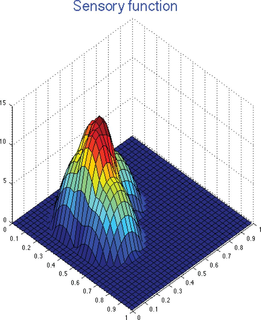
Environment’s sensory function
The parameters for the controller are
The initial path is arbitrarily designed to “zig-zag” across the environment (see Figure 3a). The region of interest in the environment is shown as a green-colored region in Figure 3. We can see how the path evolves under the IC path controller in Figure 3. After 25 time steps (Figure 3c), the path already tends to go through the region of interest, while avoiding all other regions. At 200 time steps (Figure 3f), the path clearly only goes through the region of interest. This final IC path corresponds to a local minimum of the Lyapunov-like function
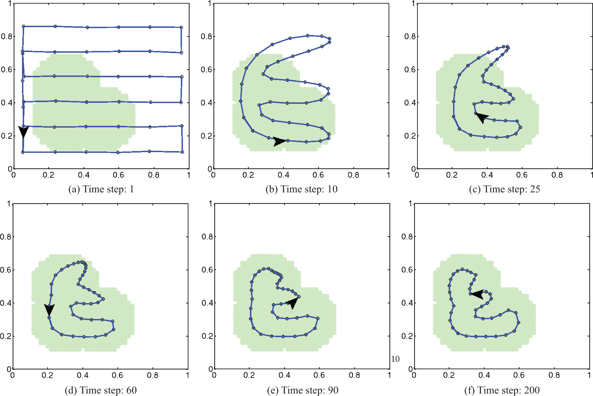
Simulated single-robot system in a known environment using the IC path controller. The path is shown as a blue line connecting all waypoints, shown as black circles. The black arrowhead is the simulated robot’s position. The region of interest is shown as a light-green-colored region.
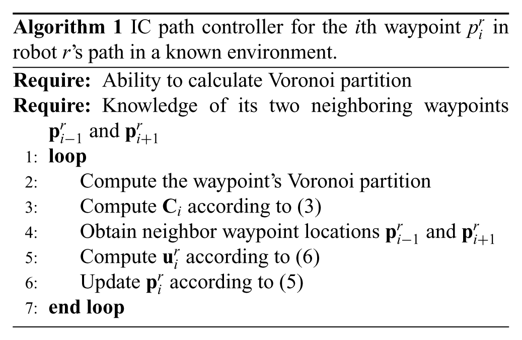
IC path controller for the i th waypoint
3.2. Discussion
The IC path algorithm’s strength lies in its simplicity and in being capable of decentralized implementation. In a fully decentralized implementation, each waypoint in the robot’s path has its own controller and performs its own calculations based only on local data. This can be accomplished by having each robot run a separate control thread for each waypoint in its path that performs the calculations in Algorithm 1.
In order to perform these decentralized calculations, each waypoint control thread must be able to compute the corresponding waypoint’s Voronoi partition. There are decentralized ways of calculating such Voronoi partition, as shown by Cortes et al. (2004). In addition, each waypoint control thread must be able to communicate to its neighboring waypoint controllers (corresponding to the previous and next waypoints in the respective path). Since the robot performing the control thread for waypoint
Another very useful feature of this controller is that, when the environment is known, it responds to changes in the environment sensory function, i.e. it works for time-varying versions of φ(
Robot path responding properly to a time-varying φ(
Finally, with respect to the controller, the selection of the parameters Ws and Wn can vary depending on the desired behavior of the system. For example, a higher Wn/Ws ratio will pull waypoints closer together, which might drive the system to a more sub-optimal configuration for sensing. If, in contrast, Wn/Ws is small, the system focuses more on the sensing task, and the waypoints in the path will be more scattered. Although in this work we do not consider vehicle dynamics, one way to indirectly impose vehicle dynamics restrictions is to increase the neighbor distance weight Wn and increase the number of waypoints in the path. This will result in smoother paths.
4. IC path controllers for unknown environments
In this section, we relax the assumption that the environment sensory function φ(
Let
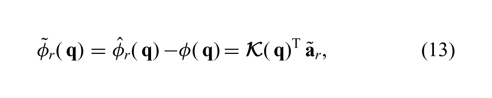
is robot r’s approximation of φ(

In addition, we can define the parameter estimate error for robot r as
4.1. Adaptive controller
We design a distributed adaptive control law for multiple robots and prove that it causes the set of paths for all robots to converge to a locally optimal configuration according to (2), while causing all of the robots’ estimates of the environment’s sensory function to converge to the real description (assuming their trajectories are rich enough). The latter is achieved by the robots integrating their sensory measurements along their trajectories and sharing their estimates with each other through a consensus term (Schwager et al., 2009). In order for the robots to properly share their estimates of the sensory function, we must make the following assumption.
Assumption 4.1. (Connected network). When working with more than one robot, i.e. N > 1, we assume that the network of robots in the system is a connected network, i.e. that the graph where each robot is a node and an edge represents communication between two nodes is a connected graph. This connected network corresponds to the robots’ abilities to communicate with each other.
Since the robots do not know φ(
where

Robot r’s parameter vector
where wr(t) is a non-negative scalar weight function for data collection (Schwager et al., 2009), whose selection is restricted such that it maintains Λ
r
and
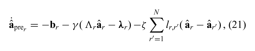
where γ > 0 is a scalar adaptation gain. The last term in (21) corresponds to a consensus term from Schwager et al. (2009) to allow the robots to share their estimates, where ζ > 0 is a consensus scalar gain, and
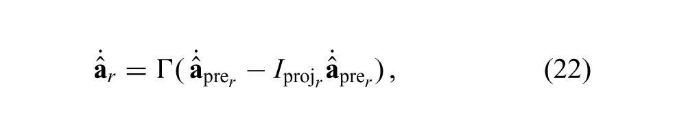
We restrict the selection of
Since
where
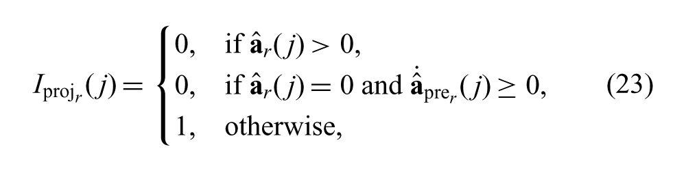
where (j) denotes the jth element for a vector and the jth diagonal element for a matrix.
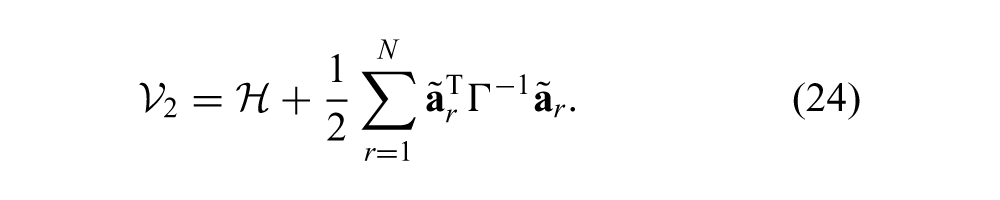
Proof. We define a Lyapunov-like function
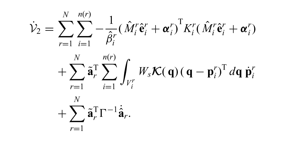
Taking the time derivative of
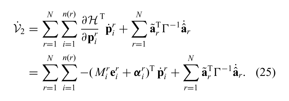
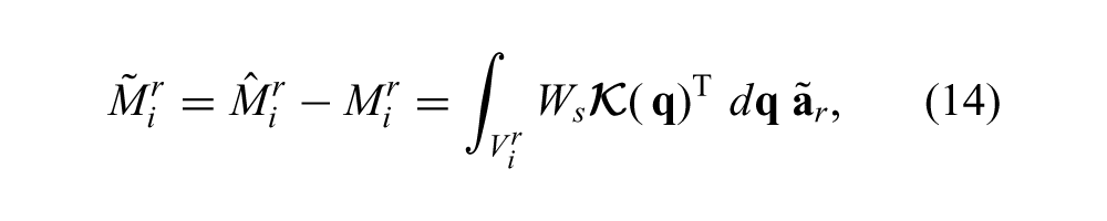
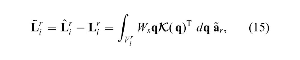
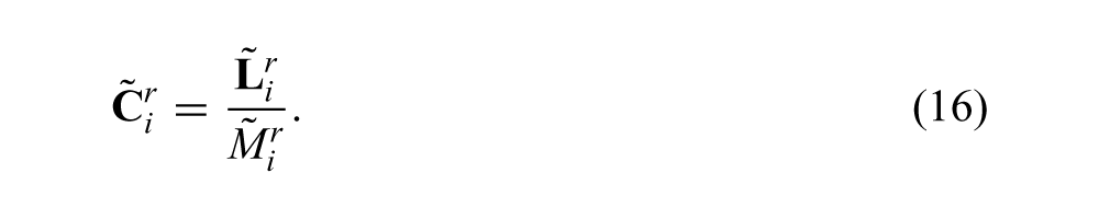
From (14), (15), (16), it is easy to check that

Plugging this into (25),
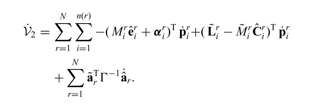
Using (14), we have
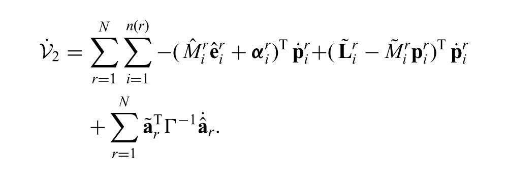
Substituting the dynamics specified by (5) and control law specified by (17), we obtain
Using (14) and (15),
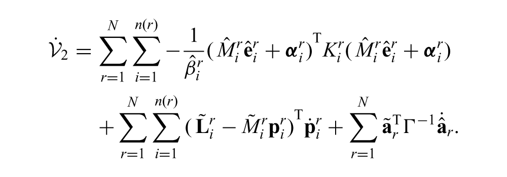
Plugging in the adaptation law from (20), (21) and (22),
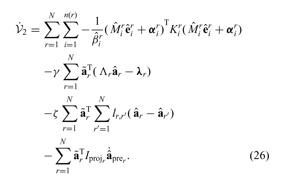
Using (18) and (19), the second term in (26) becomes
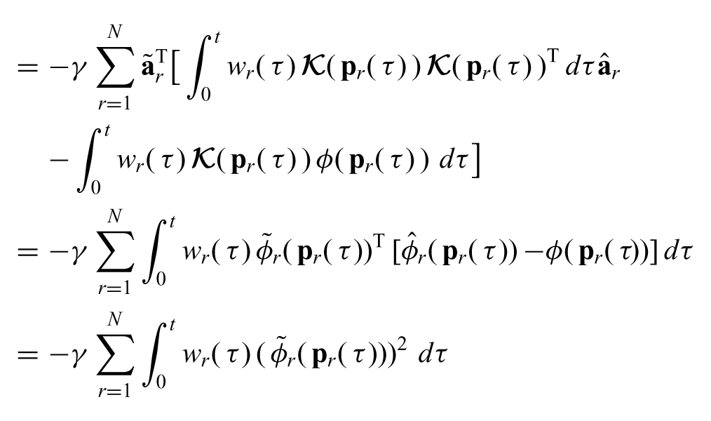
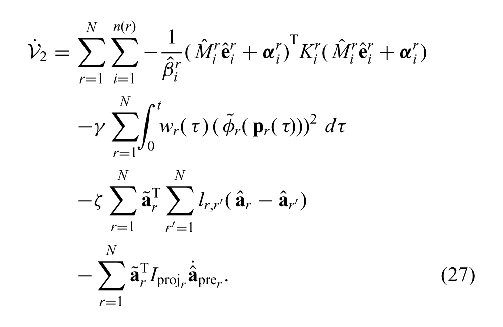
Plugging this expression back into (26) we obtain
Let
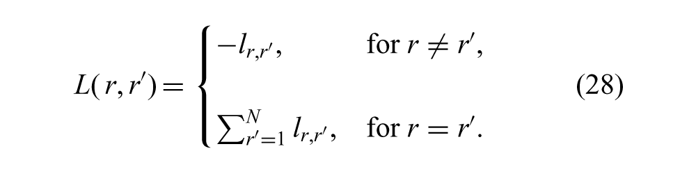
This graph Laplacian is positive semidefinite and, since our network of robots is a connected one, we know that it has exactly one zero eigenvalue whose eigenvector is

and we have that
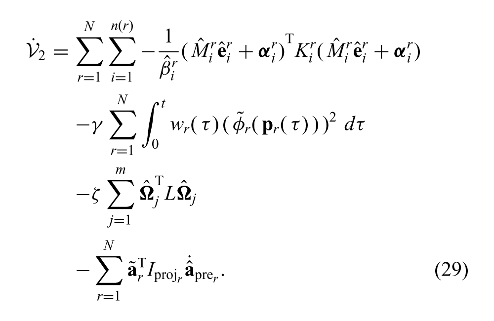
Denote the four terms in (29) as ξ1(t), ξ2(t), ξ3(t), and ξ4(t), so that
Now consider the time integral of each of these four terms,
Remark 4.3. Property (i) from Theorem 4.2 implies that the paths will reach a locally optimal configuration for sensing, i.e. an IC path, where the waypoints reach a stable balance between being close to their neighbor waypoints and providing good sensing locations according to the estimated sensory functions
Remark 4.4. Properties (ii) and (iii) from Theorem 4.2 together imply that
4.2. Data collection weight functions
The adaptation law mentioned above includes a data collection weight function wr(t) in the calculations of Λ
r
and
Another clear option is to simply use a constant for a certain amount of time, and then set the weight to zero in order for Λ
r
and
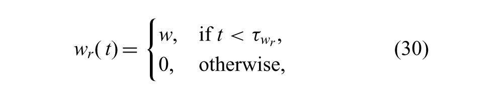
where w is a positive constant scalar, and
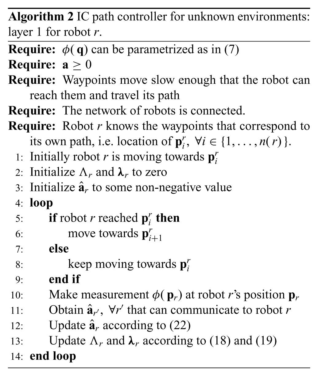
IC path controller for unknown environments: layer 1 for robot r.
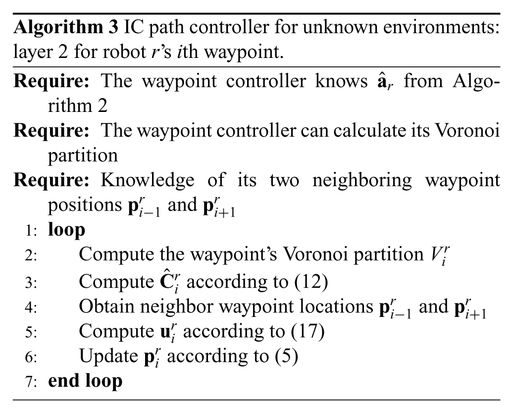
IC path controller for unknown environments: layer 2 for robot r’s ith waypoint.
4.3. Additional note on the adaptation law
As mentioned in Remark 4.4 the robots’ estimates of the sensory function will converge to the real description for the locations that they visit while the weight function is positive, but not necessarily for other locations. Hence, in order for the robots to perform the sensing/coverage task in an acceptable way, it is a good idea to provide the robots with initially rich trajectories through the environment. In our simulations and experiments we provide such rich trajectories by giving the robots initial paths that pass through most of the environment (“zig-zagging” through the environment) and we allow the robots to travel their initial paths once with the IC path controller, but with
This initial pass by the robots through their paths without editing them and using the adaptation law to make estimates of the sensory function is referred to as the learning phase. Once the robots obtain enough samples of the sensory function in order to make proper estimates of it, the robots stop taking samples in order to maintain Λ
r
and
The reader should note that this is purely an implementation detail and it is not, by any means, a requirement of the adaptive controller that we propose in this paper. For example, the separation of these two phases is not necessary if we initialize the parameter estimates
In any case, our adaptation law allows the robots to perform estimates of the sensory function online in a decentralized way with asymptotic convergence to the true sensory function guaranteed for all robots if the union of their trajectories is rich enough. This online adaptation law can especially be beneficial in some scenarios where the sensory function varies slowly in time. For such cases, a decaying exponential weight function for data collection (as specified in Section 4.2) can allow the robots to change their estimates as the sensory function changes. However, this case of time-varying sensory functions is outside the scope of this paper and will not be discussed further.
4.4. Decentralized algorithm
The IC path controller for unknown environments can be implemented in a decentralized way using the architecture shown Figure 5, which is divided into two layers. The first layer (top of Figure 5) corresponds to the robots traveling through their paths, and sampling and estimating the environment sensory function. A practical algorithm for this first layer is shown in Algorithm 2 and can be executed in a decentralized way by each robot, in the sense that each robot can execute this algorithm independently, only sharing its current parameter estimate vector to the other robots that are within communication range (i.e.
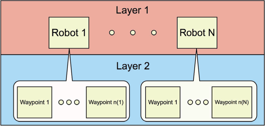
Architecture for the multi-robot system.
The second layer (bottom of Figure 5) corresponds to the waypoints being moved and placed in locally optimal locations to create IC paths. For this layer, we interpret each waypoint as having its own control thread that runs Algorithm 3. This algorithm can be implemented in a decentralized way in the sense that each waypoint control thread can execute this algorithm independently, only sharing information with their neighboring waypoint control threads and enough information for all waypoint control threads to compute their Voronoi partitions. If the robots have multiple cores, or multiple processors, the computations for each waypoint control thread can be readily parallelized for improved efficiency. 4 Alternatively, if the robots do not have the computational power to run in parallel a separate control thread for each of their waypoints, another decentralized implementation can be done if each robot individually performs its adaptation law (Algorithm 2) and the waypoint control law (Algorithm 3) in a sequential manner for all of its corresponding waypoints.
4.5. Simulated results for a single robot
In this section we present a simulation performed in MATLAB for the single-robot case (i.e. N = 1, r = 1) in an unknown environment. The robot has n(r) = 58 waypoints. The environment’s sensory function for this simulation is identical to that described in Section 3.1. The estimated parameter vector
The initial path was designed to “zig-zag” across the environment (see Figure 9a) to provide a rich initial trajectory for the robot to sample the environment. We present our results in the two phases described in Section 4.3: learning phase and path shaping phase. The learning phase corresponds to the robot traveling through its full path once, without reshaping it, in order to obtain enough samples to properly estimate φ(
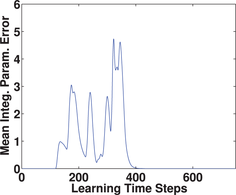
4.5.1. Learning phase
During this phase
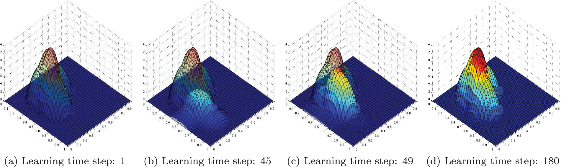
Simulated environment during the learning phase. The translucent data represents the true sensory function φ(
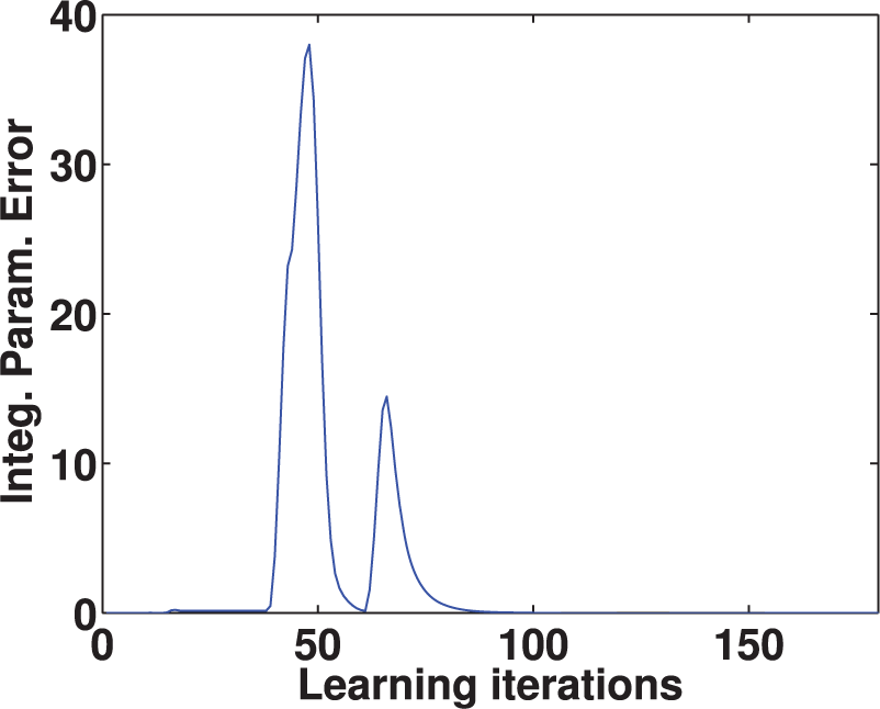
Integral parameter error.
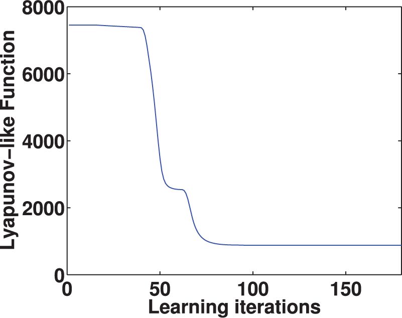
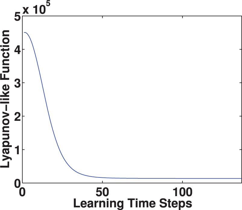
Lyapunov-like function.
4.5.2. Path shaping phase
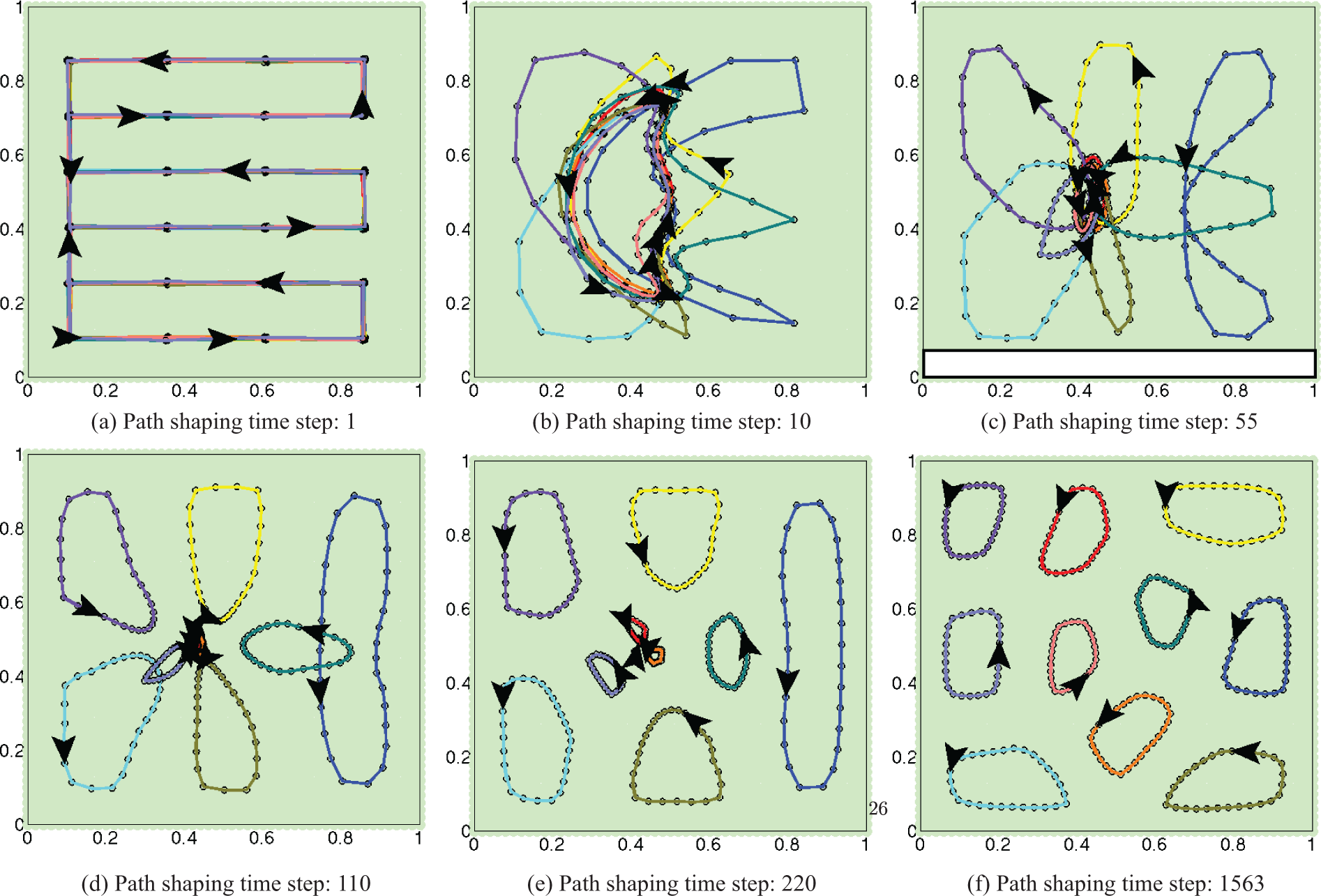
Once the robot travels through its path once (sampling and building an estimate
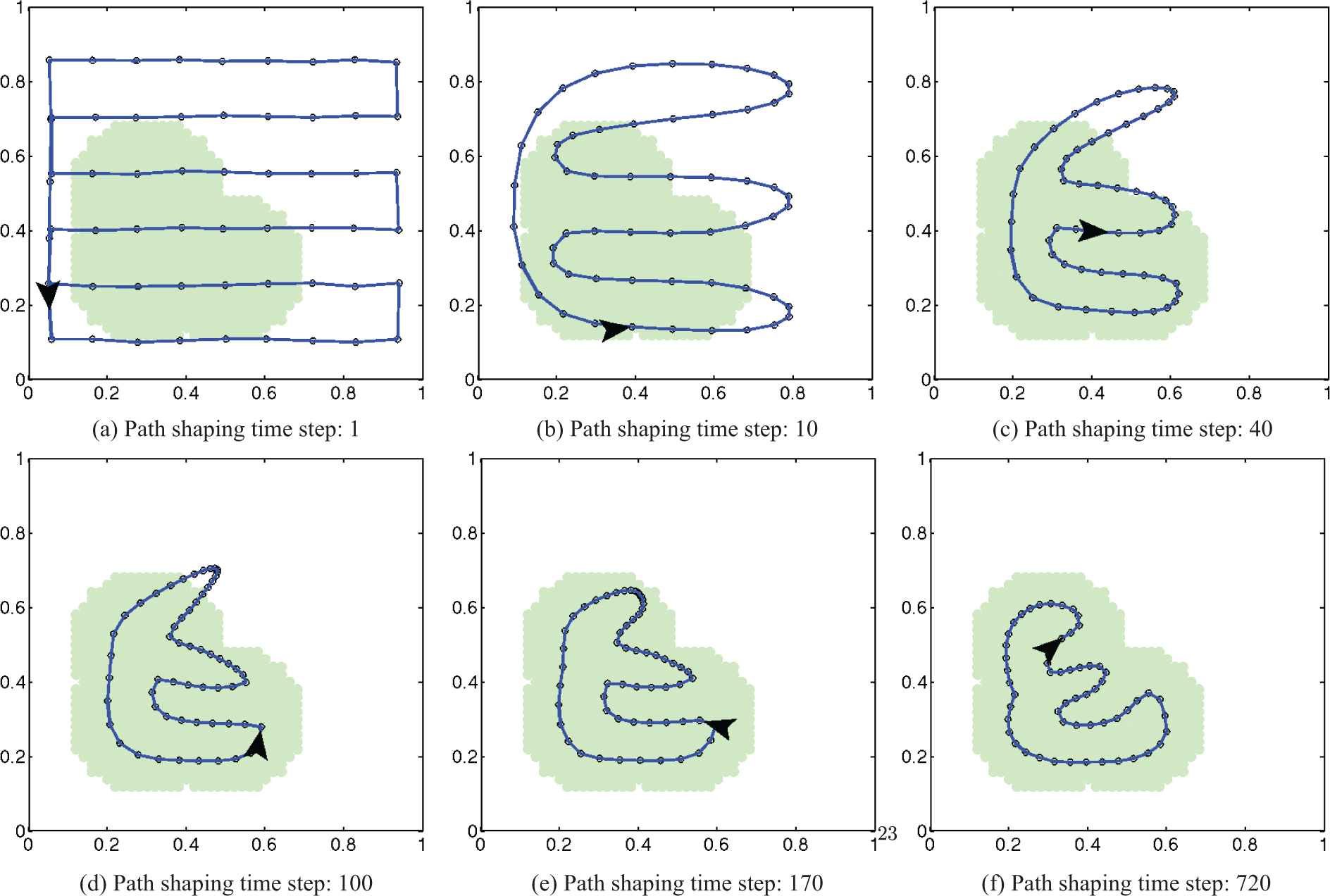
Simulated single-robot IC path controller for an unknown environment. The path is shown as a blue line connecting all waypoints, shown as black circles. The black arrowhead is the simulated robot’s position. The region of interest is shown as a light-green-colored region. As time passes, the robot’s path converges to a configuration that only focuses on the region of interest.
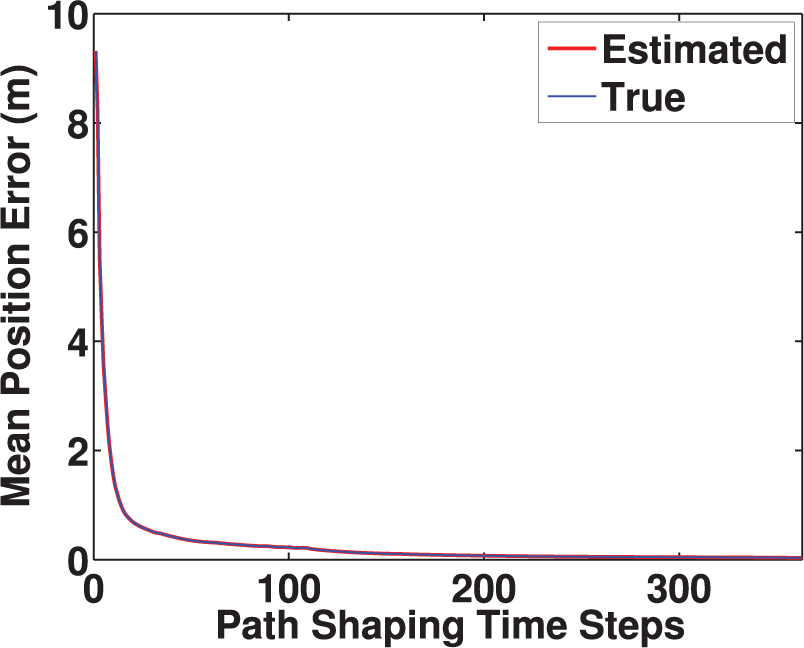
Figure 10 shows the true and estimated mean waypoint position errors, where the estimated error refers to the quantity
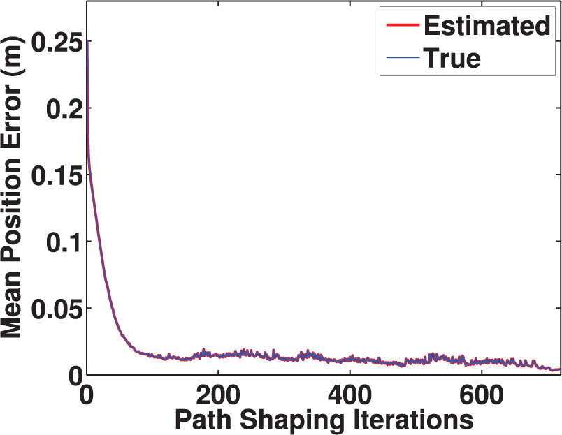
Mean waypoint position error.
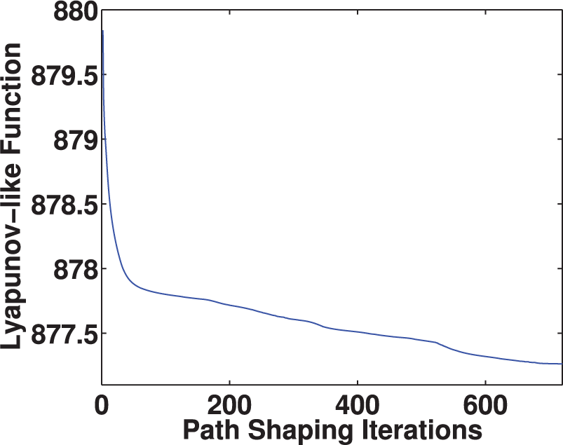
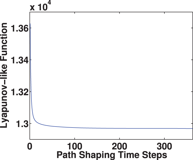
Lyapunov-like function.
4.6. Simulated results for multiple robots
In this section we present a simulation of a 10-robot system in an unknown environment using our IC path controller. This simulations, like all others, was done in a quasi-decentralized way, in which the decentralized controllers shown in Algorithms 2 and 3 were used, but in a single laptop computer. We present a case for N = 10 robots and n(r) = 28 waypoints,
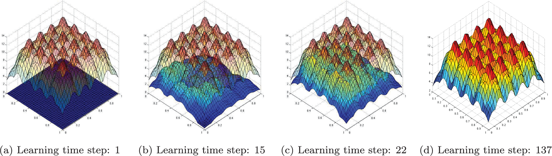
Simulated environment during the learning phase. The translucent data represents the true sensory function φ(
The parameter vector
The initial paths can be seen in Figure 17a, where all robots have practically the same “zig-zagging” initial path across the environment, providing rich initial trajectories for them to sample the environment. 5 We present results in two separate phases: (1) learning phase; and (2) path shaping phase.
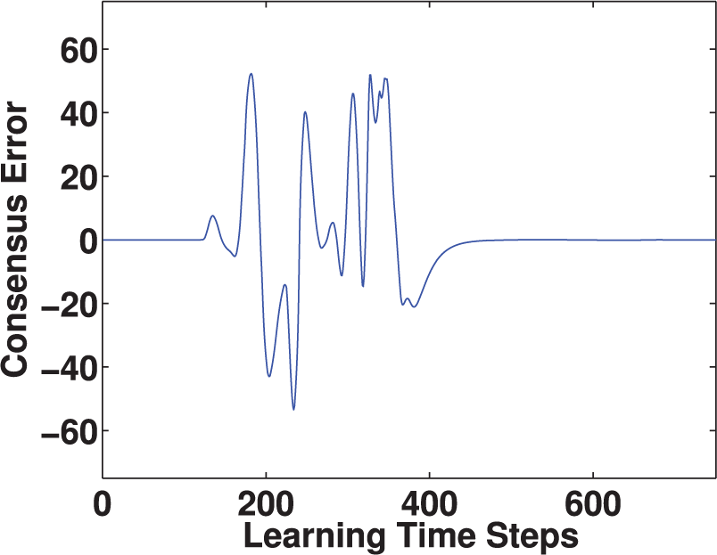
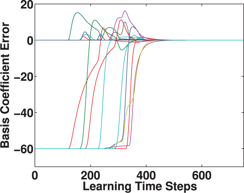
4.6.1. Learning phase
During this phase
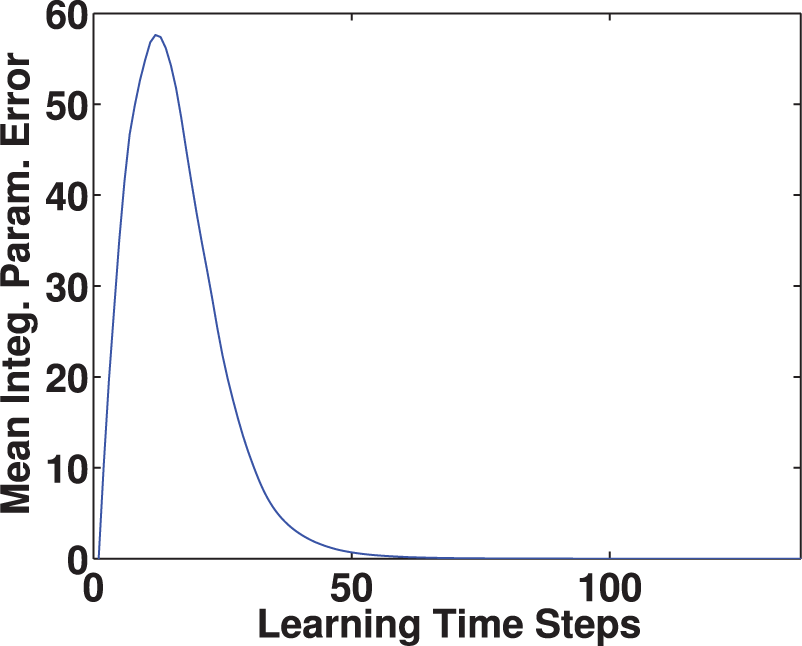
Integral parameter error.
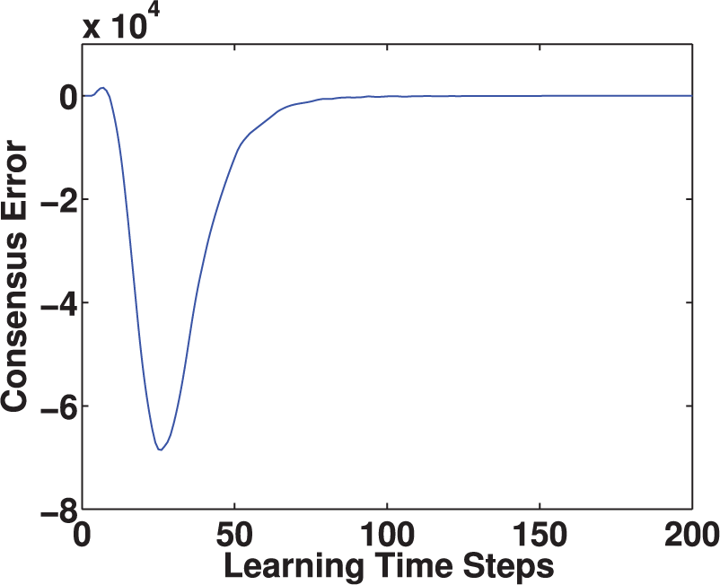
Consensus error.
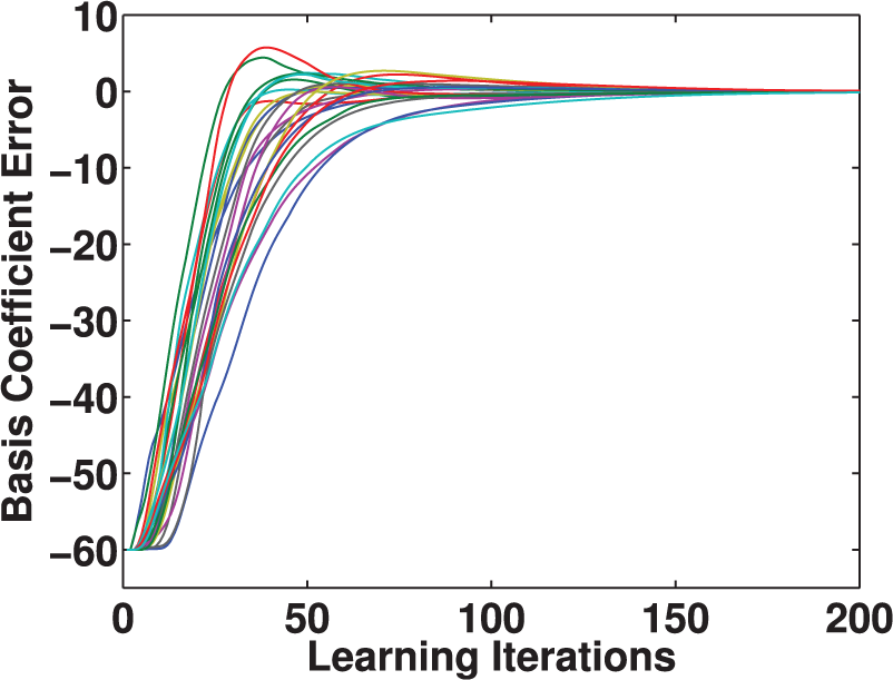
Basis coefficient error.
Lyapunov-like function.
4.6.2. Path shaping phase
After the robots travel through their paths once, sampling φ(
Simulated 10-robot system using the IC path controller. Each robot follows a path with a unique color. All robots have approximately the same initial path, as seen in (a). The black arrowheads represent the simulated robots. The region of interest, shown as the light-green-colored region, is all of the environment since φ(
Mean waypoint position error.
Lyapunov-like function.
Note that the sensory function φ(
4.7. Discussion
The IC path controller drives the robots to work together to sense/cover the regions of interest in an unknown environment. In the case seen in Figure 17, since the region of interest is the entire environment, we see that the robots’ paths spread out throughout the entire environment to cover it uniformly. This sense of teamwork seen in the robots and their paths comes as a direct consequence of the coupling that exists between them in the Voronoi decomposition. Owing to this, a robot’s path will not tend to go over the same spot that another robot’s path is already passing through because they have different Voronoi partitions. However, it is important to point out that the IC paths generated by our controller depend on the parameters Wn and Ws inserted into the controller and the initial paths assigned to each robot. We now compare some cases where such variations produce big differences in the final IC paths.
4.7.1. Variations of neighbor distance weight Wn
Due to the coupling of waypoints within each path, if the value of the neighbor distance weight Wn (or, equivalently, the ratio Wn/Ws) is high enough the paths will tend to shape in a way that creates short paths for each robot. We now present two cases with the same controller parameters, with the exception of the value of Wn. The “high Wn” case corresponds to Wn = 30 and the “low Wn” case corresponds to Wn = 3. All other parameters are the same for both cases: Ws = 150, N = 2,
The regions of interest created by these parameters are shown as light-green-colored regions in Figures 20 and 21. The initial paths for both cases are practically the same and are shown in Figure 20. The final paths, however, are very different for each case and are shown in Figure 21. The difference in final paths is mainly caused by the difference in the neighbor distance weight Wn. For both cases the IC path controller generates paths that allow the robots to sense the regions of interest. However, for the high Wn case, such a high gain provides highly attractive forces between neighboring waypoints. This causes the paths to tend to be short because the neighbor waypoints want to be close to each other. Therefore, the system evolves in a way that the environment is covered with low-length paths. In contrast, in the low Wn case, there are low attractive forces for neighboring waypoints. This causes the waypoints to be more distant to each other and focus more on the coverage/sensing task, rather than generating short paths. Depending on the application, the weights Wn and Ws can be selected to generate appropriate results. As an example, if collision is an issue, one way to possibly avoid collisions is to have a high Wn so that paths tend to not intersect each other.
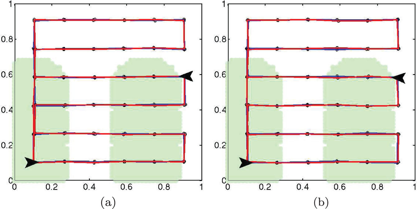
Initial paths for comparing neighbor distance weight: (a) high Wn; (b) low Wn.
Final paths for comparing neighbor distance weight: (a) high Wn; (b) low Wn.
4.7.2. Variations of initial paths
For all of the controllers that have been shown in previous sections, any initial paths for the robots can be selected. However, depending on the initial paths, the system may achieve a different set of IC paths corresponding to a different local minimum of the cost function. In this section, we provide an example to show how the initial paths can affect the local equilibrium at which the system settles to.
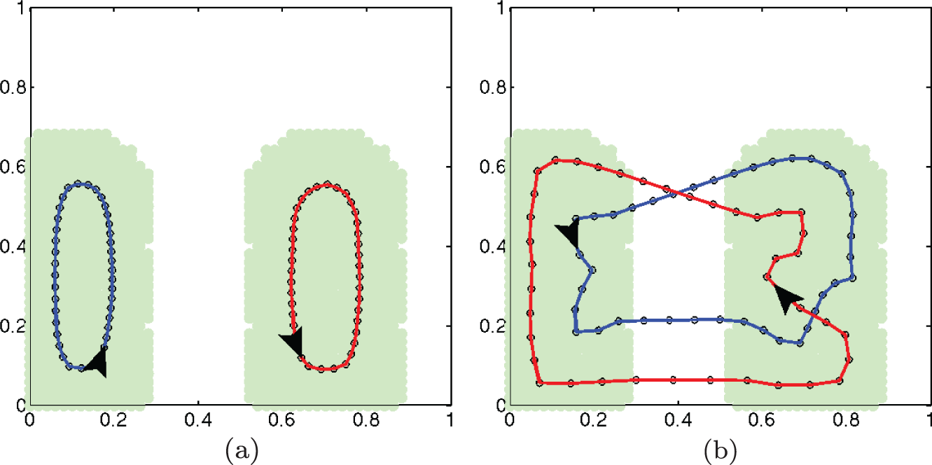
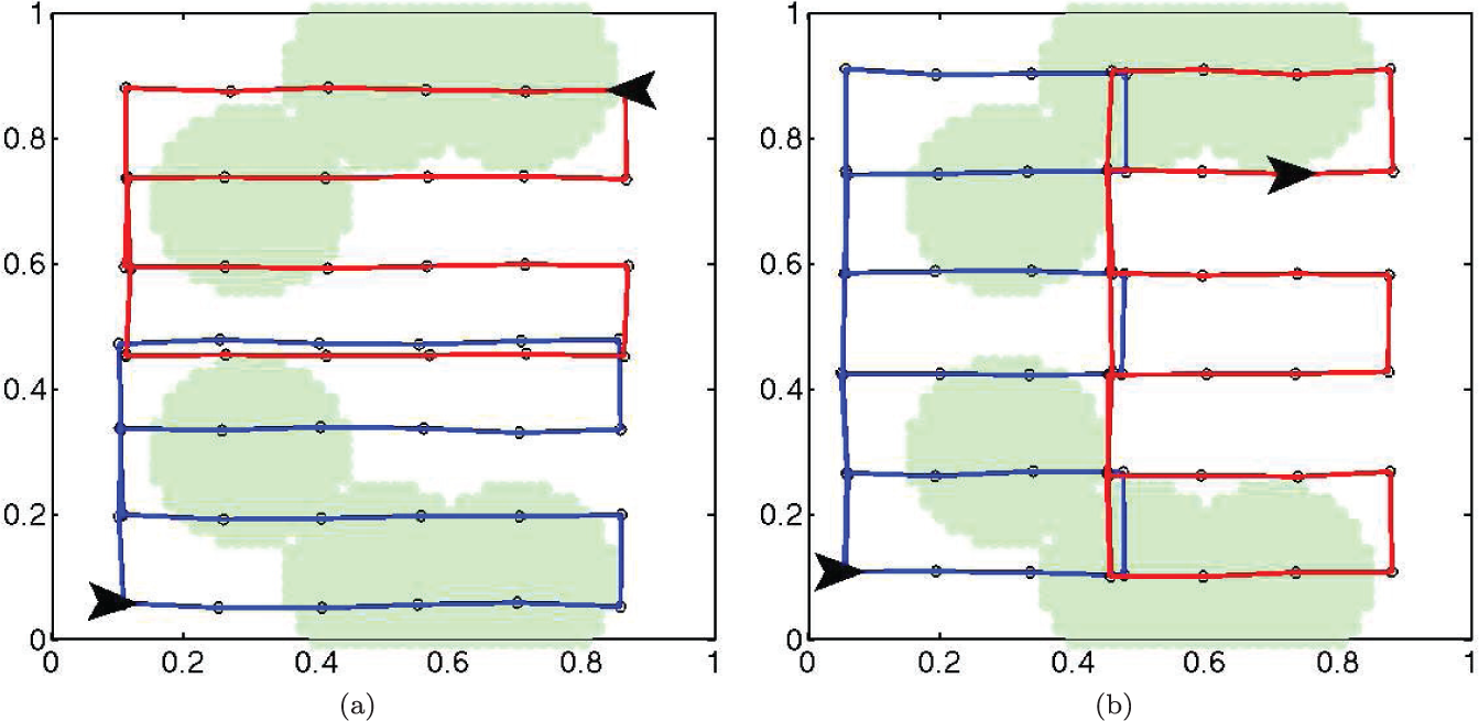
The example consists of two cases of a system with the same environment, parameters and number of robots, but with different initial paths for the robots. The parameters are: Ws = 50, Wn = 3, N = 2,
The regions of interest created by these parameters are shown as light-green-colored regions in Figures 22 and 23. The initial paths are the only difference between the two cases and these are shown in Figure 22. Consequently, the resulting final paths are very different for each case and are shown in Figure 23. More accurately, the difference in final paths is caused by a different local minimum in the cost function. From this example, it is clear that the initial paths for the robots can greatly affect the outcome of the final path shapes. Therefore, if some structure of the environment is known, it can be used to design initial paths that are more beneficial to the outcome of the system.
Initial paths for comparing initial path variations: (a) case 1; (b) case 2.
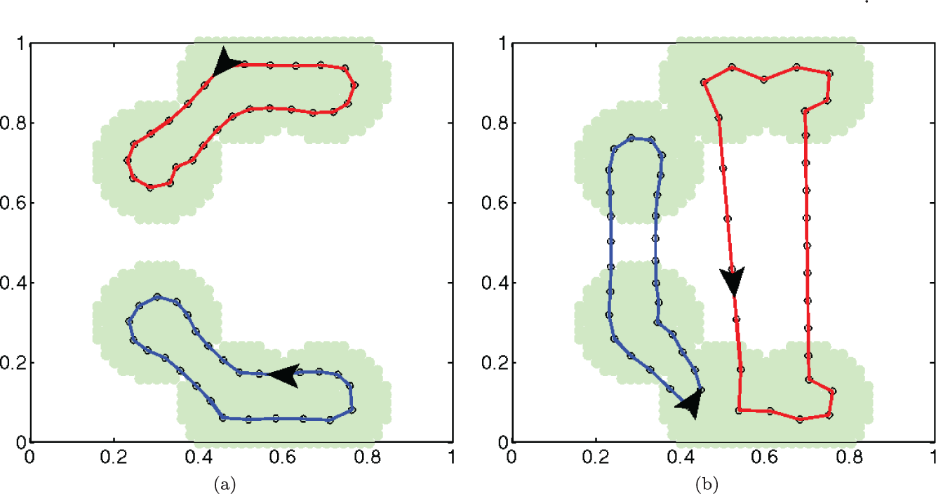
Final paths for comparing initial path variations: (a) case 1; (b) case 2.
5. Controlling the speed of the robots along the IC paths
The IC path controller only affects the locations of waypoints defining the robots’ paths. The user has the liberty of controlling the speed at which the robots travel the IC paths in order to achieve a particular task. As an example of the usefulness of exploiting this freedom, we consider the problem of persistent monitoring. In persistent monitoring we wish for the robots, each assumed to have a finite sensor footprint, to gather information in a dynamic environment so as to guarantee a bound on the difference between the robots’ current models of the environment and the actual state of the environment for all time and over all locations. Since their sensors have finite footprints, the robots cannot collect the data about all of the environment at once. Consequently, as data about a dynamic region becomes outdated, the robots must return to that region repeatedly to collect new data. More generally, if different parts of the environment change at different rates, the robots must visit these areas in proportion to their rates of change to ensure a bounded uncertainty in the estimation. The algorithm presented by Smith et al. (2011) calculates the speed of the robots at each point along a given path in order to perform a persistent monitoring task, i.e. to prevent the robots’ model of the environment from becoming too outdated. In this section, we use the IC path controller, along with the speed controller from Smith et al. (2011) to produce IC trajectories online with provable performance guarantees for persistent monitoring in unknown environments.
More specifically, Smith et al. (2011) defined the persistent monitoring problem as an optimization problem whose goal is to keep a time changing environment, modeled as an accumulation function, bounded everywhere. The accumulation function grows where it is not covered by any of the robots’ sensors, indicating a growing need to collect data at that location, and shrinks where it is covered by any of the robots’ sensors, indicating a decreasing need for data collection. This accumulation function can be thought of as the amount of dust in a cleaning task, as the difference between the robots’ mental model and reality in a mapping or estimation task, or as the chance of crime in a surveillance task. In order to apply our IC path algorithm to the persistent monitoring problem, we must treat our environment’s sensory function φ(
We assume that each robot is equipped with a sensor with a finite footprint Fr(
Following the approach from Soltero et al. (2012), the IC path controller for persistent monitoring should incorporate the stability criterion for a persistent monitoring task given the speeds of each robot at each point along their paths, referred to as the speed profiles, such that the control action increases the stability margin of the persistent monitoring task through time. Since the robots do not know the accumulation function’s rate of growth, but estimate it, each robot r’s IC path controller will work towards improving the estimated stability criterion of the persistent monitoring task, defined by Smith et al. (2011) as
where
Smith et al. (2011) gave a linear program which calculates the speed profile for each robot’s path at time t that maximizes
In order to incorporate the persistent monitoring stability criterion into our IC path controller, we must re-define the waypoints dynamics as

where
τdwell is a design parameter, and
Remark 5.1. The quantity
Remark 5.2. It is very important to note that
We now prove that the system under the new IC controller for persistent monitoring is stable.
Proof. Let
From Section 4.1, we know that second and third term in (34) converge to zero, implying (ii) and (iii), respectively, and it was shown by Soltero et al. (2012) that the first term converges to zero, implying (i).
Remark 5.4. The stability margin can theoretically worsen while
5.1. Implementation and results
We have simulated the IC controller for persistent monitoring by multiple robots in a MATLAB environment for many test cases, and we performed a physical implementation of a system comprised of two quadrotors. In this section, we present such implementation.
The implementation was performed in a quasi-decentralized way, meaning that although the algorithm is a distributed one, the computations for all waypoints and all robots were executed serially in a single computer. Hence, some of the communication procedures between distributed nodes were bypassed at the expense of a longer running time since the computations were performed serially. We used a collision avoidance algorithm for persistent monitoring from Soltero et al. (2011) in order to prevent the quadrotors from colliding.
We present a case for N = 2 robots and n(r) = 44 waypoints, ∀r. A fixed-time step numerical solver is used with a time step of 0.01 seconds and τdwell = 0.009. The region Q is taken to be the unit square. The sensory function φ(
Sensory function.
The parameters
Following the rules of a persistent monitoring task, the environment’s accumulation function grows at a growth rate φ(
The initial paths can be seen in Figure 31a, where both robots have a “zig-zagging” initial path across a portion of the environment, and, between both robots, most of the environment is initially traversed, providing rich initial trajectories for them to sample the environment. We present results in two separate phases: (1) learning phase; and (2) path shaping phase.
5.1.1. Learning phase
In this phase
Integral parameter error.
Consensus error.
Basis coefficient error.
5.1.2. Path shaping phase
In this phase
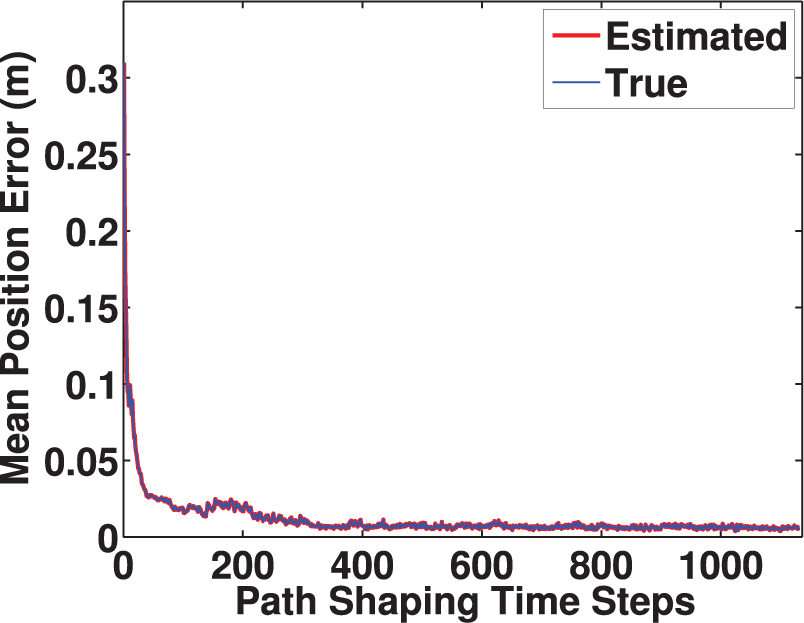
Mean waypoint position error.
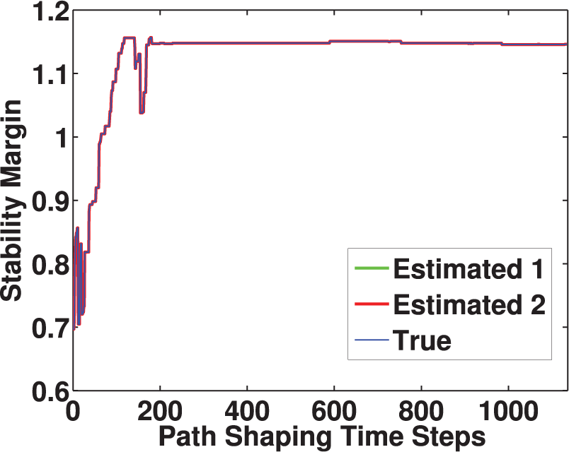
Stability margin for persistent monitoring task.
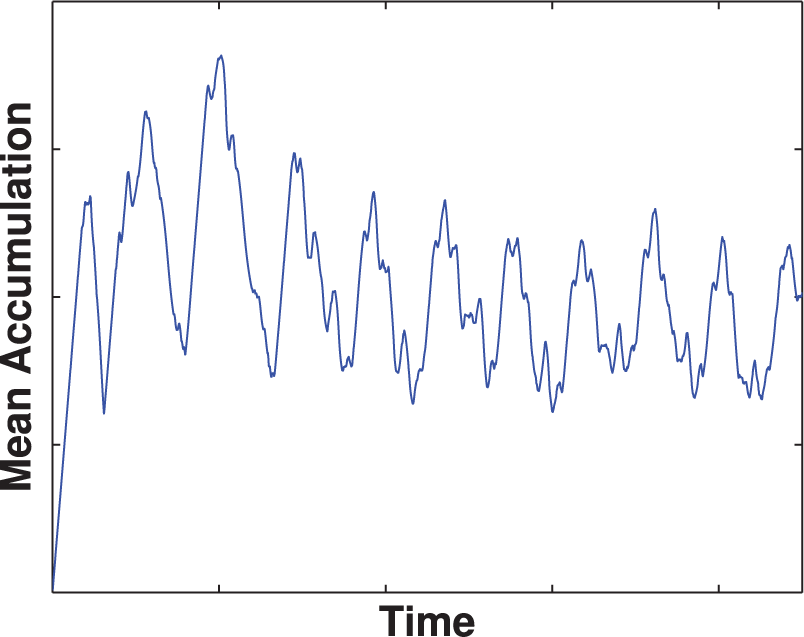
Mean accumulation function value.
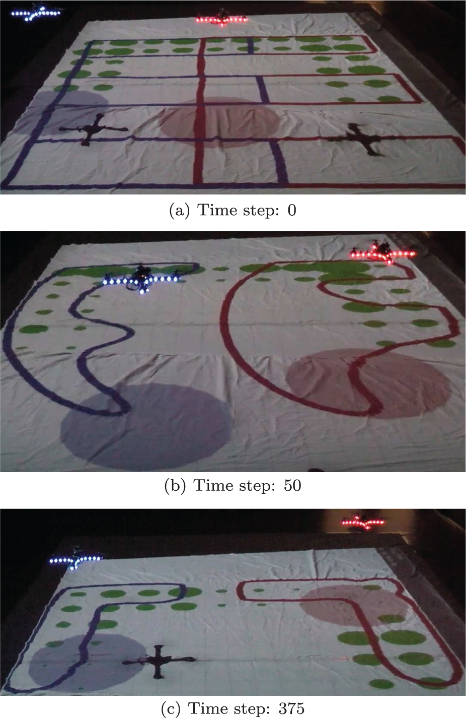
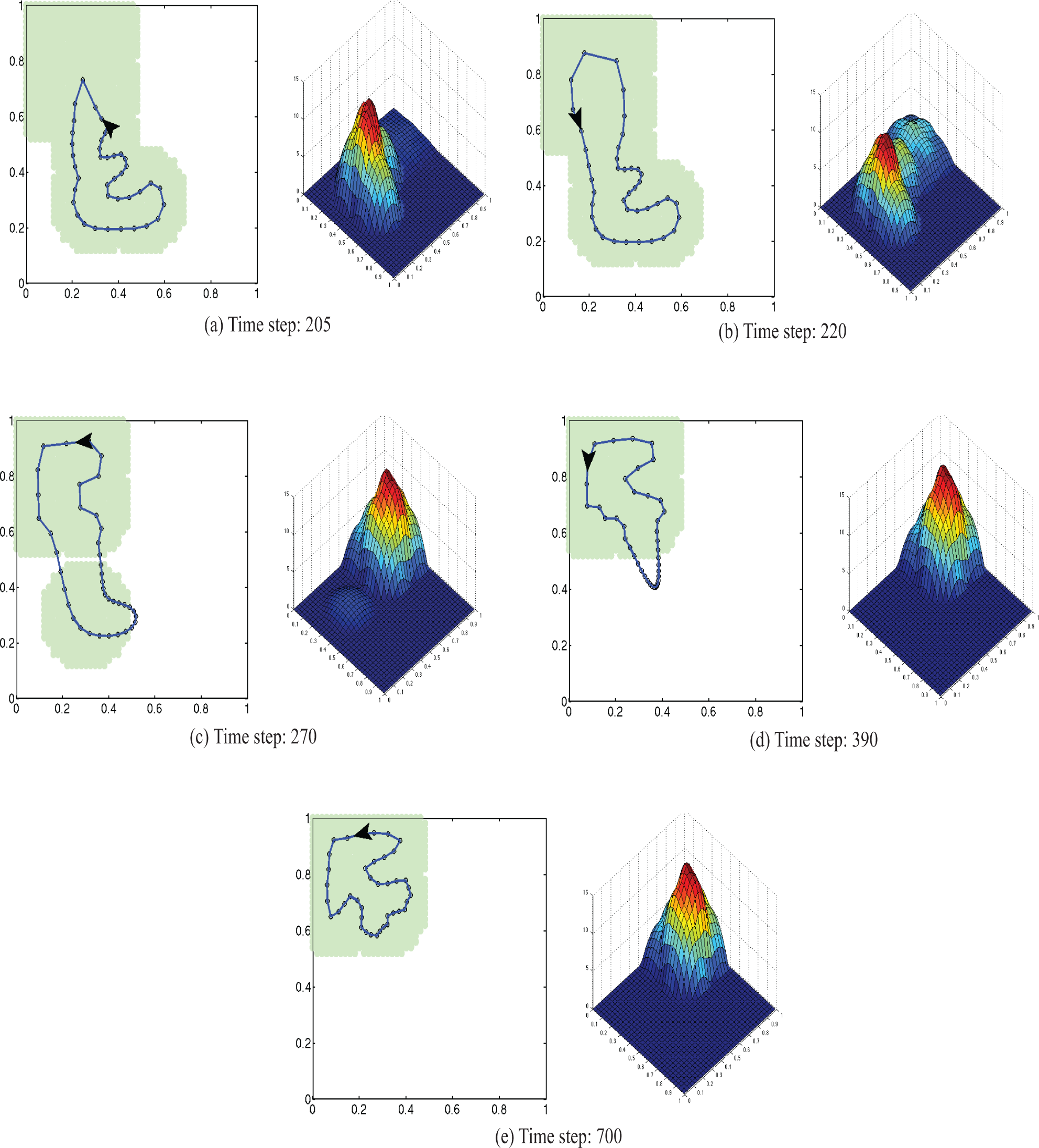
Hardware implementation of IC path controller for persistent monitoring with two quadrotors. Three snapshots of the path shaping phase at different time step values are shown. The paths, shown as the blue and red lines, connect all the waypoints corresponding to each robot. The green dots are a sample of the environment’s regions of interest and are used in the calculation of the stability margin for the persistent monitoring task. The size of a green dot represents the value of the accumulation function at that point. The robots are the blue-lit and red-lit quadrotors, and the sensor footprints for the persistent monitoring task are represented by the colored circles under the robots’ positions.
The hardware implementation was run more than 10 times, generating IC paths that are practically identical to their simulated counterparts. Since the calculations for this implementation were performed in serial, the paths reshaped much more slowly than they would in the case of a fully decentralized implementation. This experiment required approximately 3 hours to achieve a final IC path. If the implementation was performed in a fully decentralized way (each waypoint having its own control thread running in parallel), then the running time would be greatly reduced. For all cases that were studied (with or without persistent monitoring), theoretically, 7 it takes less than 20 seconds for the paths to converge to the final IC paths.
6. Limitations and future work
Although the IC path controller has very positive features such as simplicity and decentralized nature of the controller, it does have some limitations that must be mentioned. First, as has been mentioned previously, the environment’s sensory function φ(
Unlike typical search/iterative path planning methods where you can optimize a cost function encoding specific constraints, our IC path controller cannot directly encode constraints in the robots’ paths, such as length of the paths, curvature limitations, etc. Our controller can indirectly encode some of these constraints by properly selecting the parameters Ws and Wn, but there is no specific rule for determining the optimal values for such parameters. As with most problems in engineering, the user has to decide if the power of a traditional search/iterative path planner outweighs the simplicity and decentralized nature of our controller.
The IC path controllers presented here do not account for collisions when operating with multiple robots mainly because they have no information about the robots’ trajectories; they only deal with generating paths. It is only when controlling the velocity of the robots that enough information is acquired to perform collision avoidance. In this paper, when we consider the case of controlling the robot’s speed, we use a collision avoidance algorithm developed in previous work, along with some heuristics that dealt with the time-varying nature of the paths. A possible future direction for this work could be to better integrate a collision avoidance behavior in the robots under some assumptions on the robots’ speeds along the generated paths. For example, shaping the paths not only as a function of the sensory function, but also as a function of the robots’ trajectories along such paths.
The IC path controllers assume that a fixed number of waypoints are assigned to each robot. However, one could imagine that dynamically changing the number of these waypoints could improve the performance and rate of convergence in the system. The theory behind this scenario has yet to be explored and developed.
Vehicle dynamics are not considered in this paper. Hence, a vehicle with non-holonomic constraints might not be able to travel the paths generated by the IC path controller. Future work could address this issue and add constraints between neighboring waypoints that encode vehicle dynamics.
Finally, future work could focus on characterizing the sensitivity of the system under our controller to initial conditions and controller parameters, particularly to initial paths and the weight Wn. We have observed that when initial waypoint locations are very close to each other for multiple robots, the system can be very sensitive, and extremely small perturbations in the initial paths can lead to very different final paths. This is due to the sensitivity in the Voronoi partitions when generator points are too close to each other.
7. Conclusion
This paper presents a novel gradient-based path planning algorithm based on a dynamical systems approach. This approach deviates from the standard search/iterative methods that are typically used to treat the path planning problem. By doing so, we generated a very simple controller that can be implemented in a decentralized way where each waypoint in a robot’s path has its own control thread. The main difficulty of implementing this algorithm lies in the lower-level difficulty of calculating the Voronoi partitions. The proposed controller is guaranteed to reach a locally optimal solution, unlike other search/iterative methods that can only provide an approximate solution.
The proposed controller works by introducing two primitives to the waypoints’ motions. The first primitive drives the waypoints towards their Voronoi centroids, which encodes in the robots being able to cover/sense the regions of interest. The second primitive drives the waypoints to stay close to their two neighboring waypoints, i.e. the previous and next waypoints in the respective paths. This encodes in the waypoints forming closed paths. The strength of the two primitives can be customized by properly selecting the parameters Ws and Wn. The combination of the two primitives drives the waypoints to locations that correspond to locally optimal paths according to a Voronoi-based coverage cost function.
We developed the theory for the general multi-robot case. We first derived and showed results for the case where the environment is known. For this case, we saw that our assumption that the environment’s sensory function φ(
The IC path controllers provide a strong tool for robots to generate useful paths in unknown environments for any sensing task such as cleaning and surveillance. Our controller has the useful feature that the speed of a robot’s travel along its path is customizable to the specific task that the user wants achieved. As an example of this usefulness, we combined the IC path controller with a speed controller designed for persistent monitoring tasks. We proved the stability of the system under this combined controller and physically implemented it in a two-robot system tasked with performing a persistent monitoring task in an unknown environment. The controller was able to generate IC paths that were specifically useful for persistent monitoring since they locally optimized the stability criterion for the task.
Footnotes
Funding
This work was supported in part by ONR (MURI award N00014-09-1-1051), an NSF Graduate Research Fellowship (award 0645960) and The Boeing Company.