High speed locomotion for a quadrupedal microrobot

Abstract

Research over the past several decades has elucidated some of the mechanisms behind high speed, highly efficient, and robust locomotion in insects such as cockroaches. Roboticists have used this information to create biologically inspired machines capable of running, jumping, and climbing robustly over a variety of terrains. To date, little work has been done to develop an at-scale insect-inspired robot capable of similar feats due to challenges in fabrication, actuation, and electronics integration for a centimeter-scale device. This paper addresses these challenges through the design, fabrication, and control of a 1.27 g walking robot, the Harvard Ambulatory MicroRobot (HAMR). The current design is manufactured using a method inspired by pop-up books that enables fast and repeatable assembly of the miniature walking robot. Methods to drive HAMR at low and high speeds are presented, resulting in speeds up to 0.44 m/s (10.1 body lengths per second) and the ability to maneuver and control the robot along desired trajectories.

1. Introduction

Over the past several decades, significant progress has been made to enhance terrestrial robot locomotion using principles amassed from biological research. One of the key contributions from biology to legged robot designs has been the elucidation of the diverse roles of elastic elements (muscles, tendons, and ligaments) in the musculoskeletal structure of running organisms in the works of Alexander (1990) and Full and Tu (1991). All running animals, from insects to large mammals, utilize musculoskeletal springs distributed throughout their body to run efficiently and at high speeds. For example, the American cockroach reaches 1.5 m/s (50 body lengths per second) (Full and Tu, 1991), and cheetahs are capable of speeds up to 29 m/s (Hudson et al., 2011). Additionally, animals such as the cockroach display amazing maneuverability (Jindrich and Full, 1999), rapid and stable gaits over rough terrain (Full et al., 2002; Sponberg and Full, 2008), and the ability to climb vertical and inverted surfaces (Goldman et al., 2006).

By studying high performance running animals such as the cockroach, biologists have developed mathematical models for legged locomotion (Full and Koditschek, 1999) and design principles that assist in the development of legged robots. Roboticists in turn have contributed to the field with physical robot instantiations that validate biologically inspired design rules. Some key contributions include the high-performance dynamic legged robots of Raibert (1985), Saranli et al. (2001), Kim et al. (2006), Birkmeyer et al. (2009), and Hoover et al. (2008). Through the development of biologically inspired legged robots, these works have accomplished incredible tasks such as high speed locomotion (Cham et al., 2002; Birkmeyer et al., 2009; BostonDynamics, 2013; Haldane et al., 2013; Seok et al., 2013; Spröwitz et al., 2013), climbing vertical surfaces (Murphy et al., 2011), running over rough terrain (Saranli et al., 2001), and high speed maneuverability (Pullin et al., 2012).

Insect-scale mobile robots have been envisioned for several applications such as the exploration of hazardous environments, including collapsed buildings or natural disaster sites. Insect-scale robots with embedded sensors can be used in swarms that may collectively access confined spaces. These swarms could quickly search large areas to assist rescue efforts by locating survivors or detecting hazards such as chemical toxicity and extreme temperatures. In general, the benefits for reducing the scale of a walking robot include reaching confined spaces, low cost, robustness (strength to weight ratio is inversely proportional to size), and favorable scaling with regards to climbing (Trimmer, 1989).

Much of the work discussed above focuses on larger scale machines, 10 g and above, and little progress has been made in the development of at-scale insect-inspired running robots. RoACH, a 2.4 g hexapod, was developed (Hoover et al., 2008), and at the time held the title of smallest and lightest autonomous hexapod. However, RoACH’s continued development occurred at a larger scale (10 g and above). Additionally, a centipede-inspired millirobot in the Harvard Microrobotics Lab has demonstrated remarkable capabilities such as obstacle traversal and robustness to missing limbs, and has elucidated some of the mechanisms behind locomotion in many-legged animals (Hoffman and Wood, 2012).

At the millimeter and milligram scale, silicon-based walking robots have been fabricated using MEMS processes (Hollar et al., 2003). Systems at this scale have demonstrated potential benefits such as large relative payload and use of batch fabrication. However, onboard power and effective ambulation have not been achieved in a MEMS-scale device.

The focus of the work on ambulatory microrobots in the Harvard MicroRobotics lab is to develop a swarm of sub-2 g insect-inspired running robots capable of traversing any terrain. Numerous engineering challenges need to be overcome to reach this goal, beginning with the design and manufacture of an insect-scale platform; traditional macro-scale components and assembly techniques are too large, MEMS processes are too time consuming and costly, and complete off-the-shelf electronics packages for power and control that fit on a sub-2 g robot do not exist. Consequently, innovation is necessary in all aspects of robot development including mechanism design, fabrication, actuation, control, and electronics.

The focus of this paper is the mechanical design and locomotion of the fifth revision of the Harvard Ambulatory MicroRobot, HAMR-VP, shown in Figure 1. HAMR is a 1.27 g legged robot manufactured using the printed circuit MEMS (PC-MEMS) fabrication and pop-up assembly (Whitney et al., 2011) for micron to centimeter-scale systems. HAMR-VP is capable of locomotion speeds up to 44.2 cm/s (10.1 body lengths per second), and is capable of maneuverability and control at both low and high speeds. While many locomotive performance metrics are not mutually exclusive, this paper highlights aspects of HAMR-VP’s locomotion and maneuverability at low and high speeds.

Figure 1.

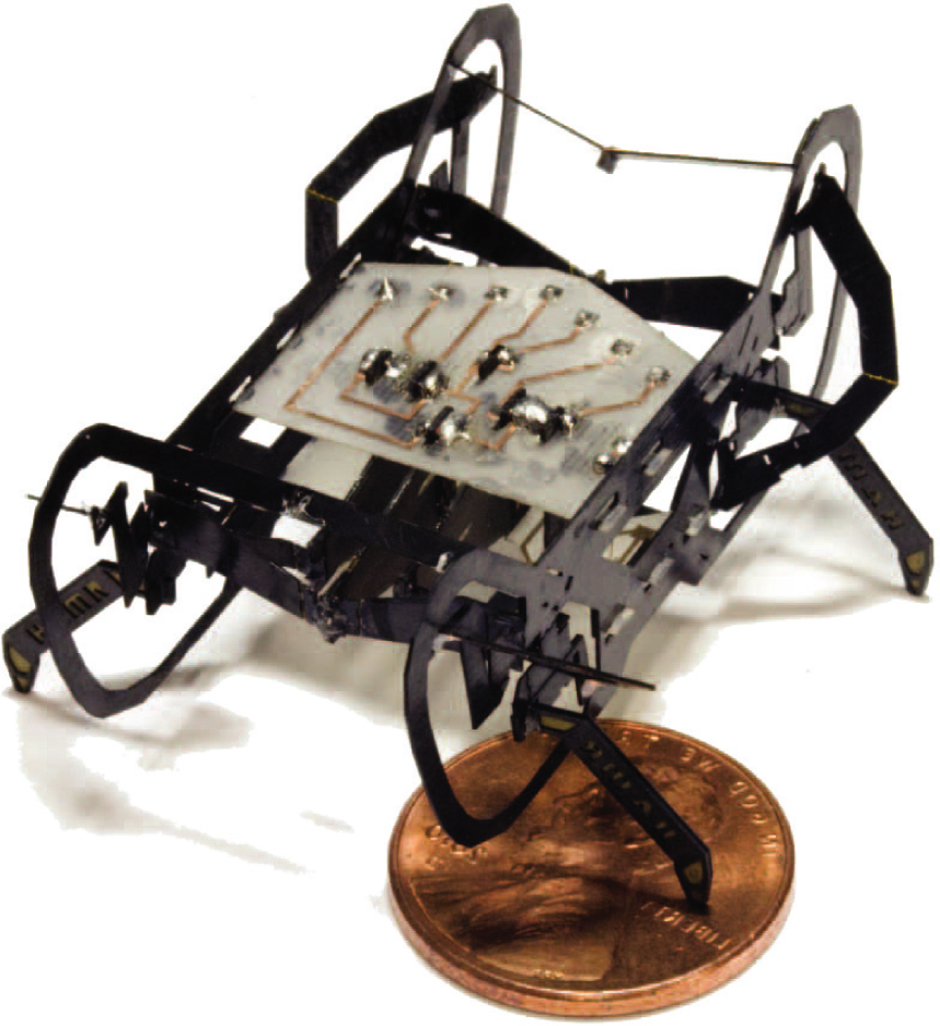
The Harvard Ambulatory MicroRobot, HAMR-VP.

2. Morphological and powertrain design

HAMR-VP has a quadrupedal morphology that was chosen to reduce manufacturing complexity over earlier hexapedal HAMR prototypes (Baisch et al., 2011; Baisch and Wood, 2011), while enabling both quasi-static and dynamic operation. This design choice was further motivated by rapidly running insects such as cockroaches, which use quadrupedal (or even bipedal) gaits at high speeds (Full and Tu, 1991). Although not ideal for stability, having only four legs does not preclude slow speed, quasi-static locomotion in an insect-scale robot. This is primarily due to a sprawled posture, which prevents the robot center of mass from ever falling outside of a statically stable support region.

The HAMR-VP design utilizes a flexure-based spherical five-bar (SFB) hip joint design (Baisch et al., 2010). The SFB enables two degrees of freedom (DOF) per leg: a lift DOF that raises and lowers the leg in the robot’s sagittal plane, and a drive DOF that provides locomotive power in the horizontal (ground) plane. The two-DOF hip joint maps decoupled inputs from two optimal energy density piezoelectric bending bimorph actuators (Wood et al., 2005) through flexure-based four-bar transmissions to a single leg (see Figure 2). An empirical study of the HAMR powertrain is described in a previous publication (Ozcan et al., 2014) where actuator and transmission parameters were selected to maximize payload and provide an adequate step height. The drive DOF uses the same parameters as the lift DOF to simplify the design and allow for interchangeable actuators. While HAMR-VP incorporates the design elements from this study, the scope of this paper is on design for pop-up assembly and characterizing the performance and control of HAMR-VP.

Figure 2.

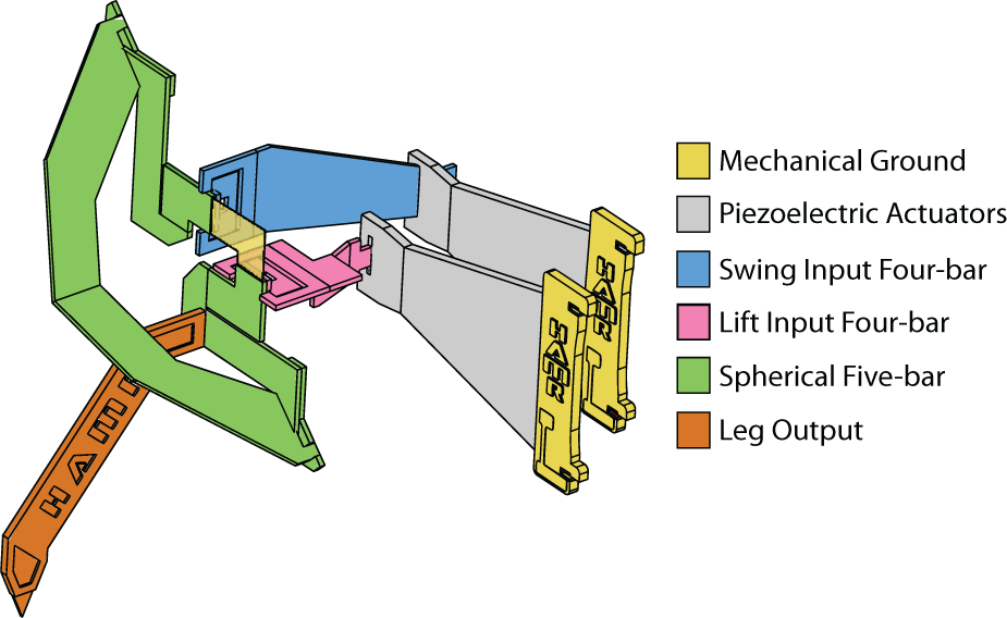
Schematic of the HAMR-VP powertrain. Power from two decoupled piezoelectric bending bimorph actuators is mapped through four-bar transmissions to a two-DOF SFB hip joint. The hip joint maps two decoupled inputs to a single leg.

Pop-up assembly enables the manufacture of complex millimeter-scale mechanisms; however, there are still a number of design and complexity tradeoffs to consider. A two DOF leg is chosen for HAMR over fewer (one) DOF legs because a one DOF leg would preclude quasi-static locomotion (see Section 4.2) which requires elliptical stepping trajectories that are unachievable using linear mechanical elements (actuators and flexures). The tradeoff for increased actuated DOFs is a substantial increase in mechanism mass and complexity. Design and manufacturing complexity as well as overall robot mass is reduced in HAMR-VP by asymmetrically coupling the drive DOFs of contralateral legs; when the front (rear) left leg swings forward, the front (rear) right leg swings rearward, and vice versa. This coupling scheme reduces the nominal eight DOFs to a total of six actuated DOFs: a front drive DOF, rear drive DOF, and four lift DOFs. This configuration supports a variety of gaits for maneuverable, quasi-static, and high-speed locomotion.

3. Design for manufacturing and pop-up assembly

A primary goal of implementing pop-up assembly into the HAMR-VP design is to improve manufacturing tolerances and thus locomotion performance. The PC-MEMS lamination process has tolerances on the order of 1–10 μm, limited by the resolution of the laser micromachining step and jig alignment precision. Therefore, prototype fidelity is highly dependent on the precision of component assembly. In an ideal case, zero manual assembly steps are required through design of devices that emerge from a single laminate (Whitney et al., 2011; Sreetharan et al., 2012). Unlike those devices, the HAMR-VP design does not implement a fully monolithic assembly process; it has 13 components to allow modularity of actuators and legs, two topics of concurrent research. The result of this new design and manufacturing process is a robot that is easy to manufacture with consistent locomotive performance that motivates and enables a diverse set of research questions for insect-scale robot locomotion and terramechanics.

Laminate composition. Mechanical components of HAMR-VP are manufactured using the PC-MEMS laminated fabrication paradigm (Whitney et al., 2011). While a diverse set of materials can be used with the PC-MEMS manufacturing process, components of the robot presented here consist of multiple five layer standard linkage laminates (SLL): a 25 μm Kapton flexure at the laminate mid-plane, two rigid three-ply [0, 90, 0] carbon fiber exterior layers (YSH-50 fibers with RS-3C resin), and two sheets of acrylic adhesive to bond the three functional layers. Designing HAMR-VP with pop-up assembly requires 23 material layers, which compose four standard linkage sub-laminates (five layers each). Subsequent linkage sub-laminates are bonded using tack-bonded acrylic adhesive (three layers), a bonding process that enables small “islands” of adhesive rather than continuous sheets (Whitney et al., 2011). See Figure 3 for a cross-sectional view of the HAMR-VP laminate composition.

Figure 3.

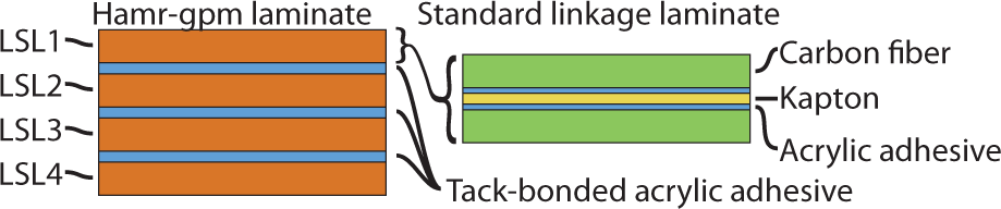
The HAMR-VP laminate stack consists of 23 material layers: four standard linkage sub-laminates (five layers each) and three layers of tack-bonded adhesive to bond subsequent linkage laminates.

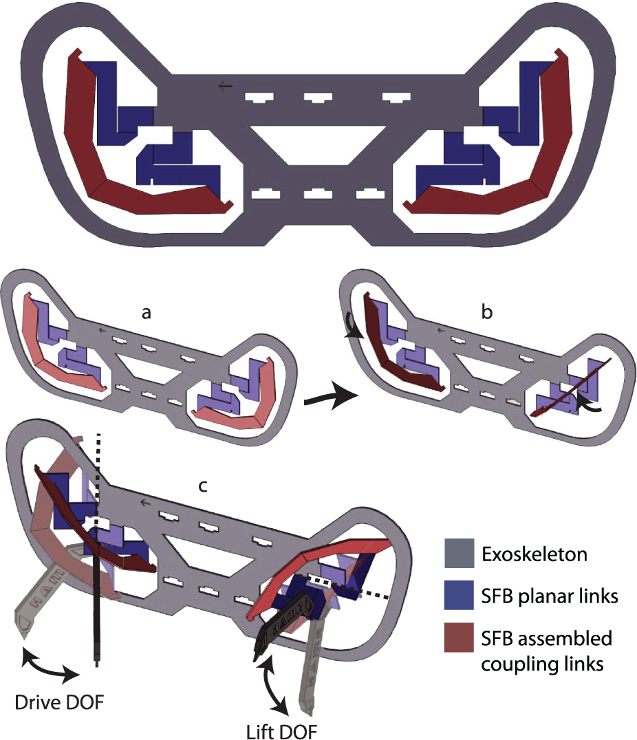
Spherical five-bar sub-laminates (LSL1 and LSL4). The pop-up HAMR-VP design utilizes the monolithic SFB joint design from Sreetharan et al. (2012) and Teoh and Wood (2013). This SFB design can be fabricated from a single linkage laminate, rather than from multiple components as in previous HAMR prototypes (Baisch et al., 2011) (see Figure 4). Thus, manufacturing tolerances are improved and assembly is easier than manual techniques; each hip only requires one 90° fold to deploy the two links that couple the lift and drive DOFs. Each SFB is folded manually during final assembly of the robot, but this is trivialized by features that constrain joint limits to exactly 90°.

Figure 4.

HAMR-VP uses a monolithic SFB hip joint design introduced in Sreetharan et al. (2012). The outer linkage sub-laminates of HAMR-VP, LSL1, and LSL4, are composed of the four SFBs. Here, LSL4 and its two SFBs are shown as a flat laminate (a), after deployment by a 90° fold (b), and with two legs to diagram the lift and drive DOFs (c).

In the HAMR-VP material layup, two outer linkage sub-laminates labeled LSL1 and LSL4 are comprised of the four SFB hip joints. The laminate is orientated such that the robot pops-up laterally, meaning the center of the material laminate (layer 13 of 23) is also the robot sagittal midplane. Therefore, LSL1 (the robot’s right side) and LSL4 (the robot’s left side) are symmetric.

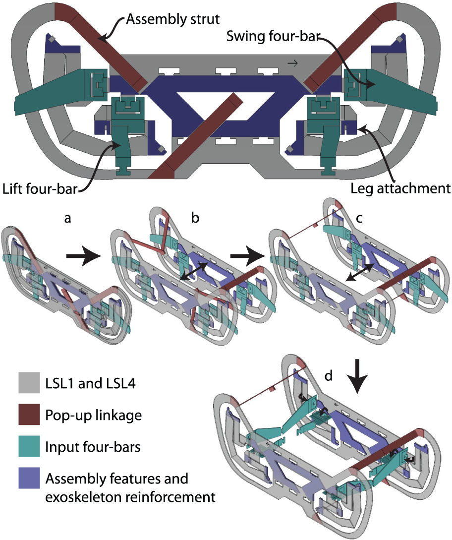
Input four-bar and pop-up strut sub-laminates (LSL2 and LSL3). Linkage sub-laminates LSL2 and LSL3, also symmetric about the robot mid-plane, are comprised of the eight four-bar transmissions between each actuator and SFB, folding struts for pop-up assembly, and additional assembly features (see Figure 5). Four-bar transmissions are adhered to the SFB via tack-bonded acrylic adhesive. Each four-bar transmission is deployed with a simple 90° fold, similarly to the SFBs, and mated to its respective actuator output during final assembly.

Figure 5.

Sub-laminates LSL2 and LSL3 comprise the pop-up assembly linkages, four-bar transmissions, and additional assembly features. The released pop-up linkage assembly (a) allows separation of the two robot halves, LSL1 and LSL4 (b,c). After pop-up assembly, the eight input four-bars are deployed by 90° folds (d).

Three parallel assembly struts forming a Sarrus linkage enable pop-up assembly of HAMR-VP by allowing separation of the right (LSL1 and LSL2) and left (LSL3 and LSL4) halves of the robot in a single DOF (see Figure 5). The assembly linkages constrain the pop-up motion such that LSL1 and LSL4 remain parallel and traverse a straight line during assembly. The robot is deployed when the assembly struts become fully extended and are orthogonal to LSL1 and LSL4. Each strut is fixed on either end to the outer linkage sub-laminates (LSL1 to LSL2 and LSL4 to LSL3), and at the laminate mid-plane (LSL2 to LSL3) using tack-bonded acrylic adhesive.

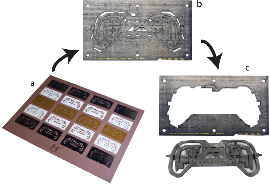
Laminate manufacturing process. The manufacturing process for HAMR-VP (see Figure 6) begins by machining the 23 material layers using a diode-pumped solid state (DPSS) laser, followed by pin-alignment and stacking on a jig. The laminate is cured under heat and pressure, then the robot outline and pop-up DOF are released from the surrounding material using the DPSS laser.

Figure 6.

Manufacturing process for the pop-up HAMR-VP. 23 material layers, 20 continuous sheets (a) and three tack-bonded adhesive layers, are laser machined and laminated to produce the structure in (b). A second laser-machining step releases the HAMR-VP structure (c), allowing initial pop-up assembly.

Final assembly. Once released, completion of HAMR-VP requires manual assembly of the 13 components (see Figure 7). First, the exoskeleton is completed by fully expanding the pop-up DOF and inserting two copper-clad FR4 circuit boards, which trace off-board power and control electronics to the actuators. The circuit boards are populated with six piezoelectric cantilever actuators, using solder as a mechanical and electrical interface. Each input four-bar transmission is then assembled by making a 90° fold and affixing its input link to the distal end of its respective actuator. The robot is completed once SFB coupling links are folded 90° to their joint stop, and four carbon fiber legs are attached to the hip joints. As previously mentioned, legs and actuators are modular, and therefore the leg-to-hip and actuator-to-four-bar bonds are made using a thermoplastic adhesive. All other bonds, such as at 90° transmission folds, are made with permanent cyanoacrylate glue.

Figure 7.

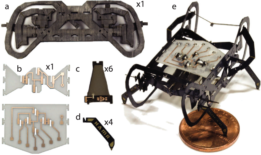
The HAMR-VP pop-up laminate (a) is fully opened and constrained with two copper-clad FR4 circuit boards (b). The circuit boards, which trace from off-board power and control electronics, are populated with piezoelectric actuators (c) using solder for electrical and mechanical connection. Four-bar transmissions and SFBs are deployed, followed by attaching four legs (d) to their respective SFB output to finalize assembly of HAMR-VP (e).

4. Straight line locomotion

4.1. Drive signal parameterization

Each of HAMR-VP’s piezoelectric actuators is voltage-driven using an alternating drive configuration consistent with Karpelson et al. (2012), thus requiring bias, ground, and signal voltages. To simplify electrical inputs, all six actuators share a single bias and single ground rail. Therefore, eight unique voltages are required for the robot: constants V_Bias and ground, and six drive signals, V_s_1–6. Voltages are generated by off-board electronics, using a controller written in Matlab and Simulink and interfaced with an xPC Target real-time testing environment. Bias and control signals are then amplified to high voltages (up to 250 V) and fed to the piezoelectric actuators by 52-gauge copper wire.

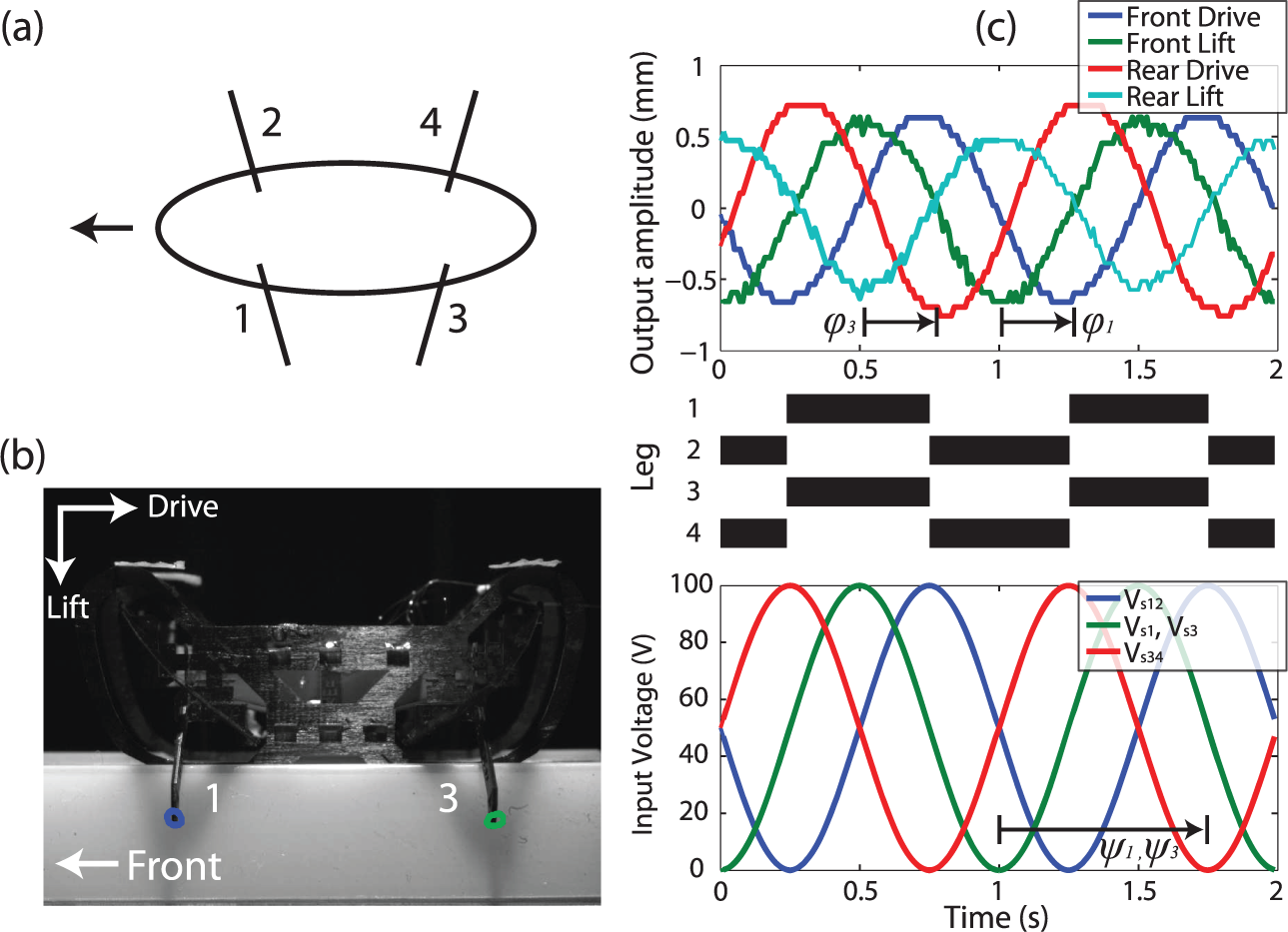
Sinusoidal inputs to HAMR-VP are defined $V_{s i} = V_{0 i} + \frac{V_{a i}}{2} \sin (2 π f_{i} t + ψ_{i})$ with parameters: mean voltage V₀, peak-to-peak amplitude V_a, frequency f, and phase ψ_i. Input parameter subscripts indicate their affected leg(s) according to the convention in Figure 8(a); independent lift DOF signals are V_s₁, V_s₂, V_s₃, V_s₄, and coupled drive signals are V_s₁₂, V_s₃₄.

Figure 8.

HAMR-VP’s actuator input and leg convention. Six actuators are driven by sinusoidal inputs $V_{s i} = V_{0 i} + \frac{V_{a i}}{2} \sin (2 π f_{i} t + ψ_{i})$ (c). Parameter subscripts indicate the leg(s) that each actuator affects, using the convention in (a). Two 90° out of phase sinusoidal inputs to the lift and drive DOFs (c) cause a roughly circular output (b). Actuating the front and rear drive DOFs 180° out of phase creates a trotting gait (c), although here it is used for quasi-static operation as well; black bars in (c) represent the footfall pattern of HAMR-VP’s nominal gait. Due to symmetry between front and rear lift powertrains (actuators face in opposite directions), in-phase lift DOF inputs to legs 1 and 3 have outputs 180° out of phase (c).

For straight locomotion, the parameter space was reduced from 25 (V_Bias and six actuators with four parameters each) to 12 by enforcing symmetry between the front/rear and left/right sides of the robot. The twelve input parameters for straight locomotion are summarized in Table 1. Nominal parameter values were chosen for a walking gait similar to a trot. Drive inputs were therefore 180° out of phase to generate in-phase diagonal legs with a footfall pattern shown in Figure 8(c). A quick study varying lift input phase found the fastest locomotion at ψ₁ = ψ₂ = ψ3 = ψ₄ = 270°, and was therefore chosen as the nominal value.

Table 1.

Input parameters for straight locomotion.

Parameter	Description	Nominal value
V _Bias	Actuator bias voltage (V)	200 V
F	Gait frequency (Hz)	1–98 Hz
V _0-Li	Lift DOF signal mean (V)	100 V
V_a _-Li	Lift DOF signal peak-to-peak amplitude (V)	200 V
V _0-Dr	Drive DOF signal mean (V)	100 V
V_a _-Dr	Drive DOF signal peak-to-peak amplitude (V)	200 V
ψ _1,2,3,4	Lift signal phases (°)	270°
ψ ₁₂	Front Drive DOF phase (°)	180°
ψ ₃₄	Rear Drive DOF phase (°)	0°
D _1,2,3,4	Lift DOF signal duty cycle (%)	50%
D _12,34	Drive DOF signal duty cycle (%)	50%

4.2. Quasi-static locomotion

Locomotion studies performed on HAMR-VP are in two regimes: a ‘quasi-static’ regime and a ‘dynamic’ regime. The difference between the two regimes is primarily in the effect of powertrain dynamics on locomotion. In the quasi-static regime, a nominal and ‘un-tuned’ set of actuator inputs are chosen to drive the robot based purely on leg kinematics. This regime is characterized by discrete steps and a velocity bounded by the product of stride length and frequency. Frequencies corresponding to this motion are experimentally found to be below 10Hz. Above 10Hz, however, the actuator inputs are tuned to compensate for dynamic powertrain effects characteristic of a second order spring mass system. Actuator inputs are tuned based on the individual powertrain dynamics of each leg and are determined independently from the overall robot rigid body dynamics.

4.2.1. Quasi-static locomotion results

Here, walking results are presented for locomotion using up to 10 Hz gait frequency, in which powertrain force and displacement outputs were unaffected by frequency. The experimental setup used to obtain locomotion results consisted of a card stock walking surface and overhead camera (PL-B741F, Pixelink). Three markers on the robot were tracked using custom post-processing software to obtain robot center of mass position (x, y) and orientation (Θ). Velocities were obtained by numerical differentiation of position and orientation with respect to time. HAMR-VP’s legs are modular in order to investigate leg compliance, traction, and adhesion in future work. In this work, legs are simply made from rigid carbon fiber, allowing them to slip during locomotion.

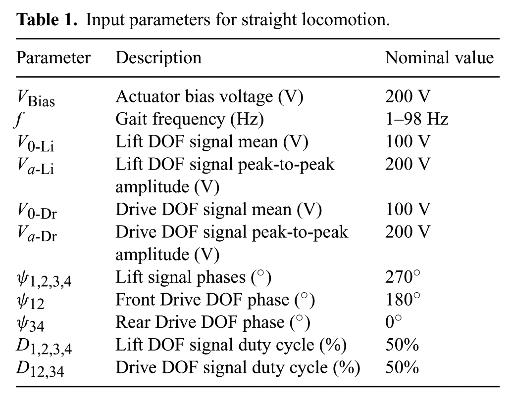
Figure 9 summarizes locomotion performance of HAMR-VP in the quasi-static regime. Speed measurements in Figure 9(a) represent average forward velocity (as defined by a body-fixed coordinate frame) ignoring lateral and rotational motions. The results show a nearly linear relationship between frequency and velocity, excluding a small deviation from 4–6 Hz. The slope of a linear fit to this data approximates the per-cycle stride length of 4.4 mm (2.2 mm per step). In air, the per-step stride length of HAMR-VP is 2.7 mm. This represents a quasi-static speed limit for HAMR-VP without slipping and is plotted with the data in Figure 9(a). The measured walking speed in this regime is, on average, 19% less than the quasi-static speed limit. This decrease in speed is due to slipping and other foot–ground interactions. The goal of work in the dynamic regime will be to exceed the quasi-static speed limit.

Figure 9.

Straight, quasi-static locomotion results of HAMR-VP. Trials were conducted from 1–10 Hz, recording speed (a). Data in (a) represents average trial velocity, defined by a body-fixed coordinate frame (ignoring lateral and rotational movement). Error bars indicate maximum and minimum velocity across three trials. The linear fit to the data for walking on the ground is 19% less than the projected quasi-static speed limit of HAMR-VP (from the measured stride length in air). Additionally, payload capacity was measured by adding discrete 225 mg masses to the top of HAMR-VP and recording velocity (b).

Payload. The effects of payload on HAMR-VP’s locomotion performance were obtained by adding up to 1.35g (106% of the body mass) to the robot in 225 mg increments. The results in Figure 9(b) predictably indicate a decrease in velocity with increasing payload. Above 1.35g payload, HAMR-VP exhibited stick-slip locomotion; feet did not leave the ground, but reduced friction in the swing phase is enough to cause net forward locomotion. Therefore, locomotion with 1.35g or greater payload could only occur on perfectly flat terrain. Based on HAMR3 specifications (Baisch et al., 2011), the estimated range of onboard electronics and battery mass is 600–700 mg, resulting in a 6–18% predicted decrease in quasi-static velocity.

Power. Total electrical power of the six HAMR-VP actuators was measured at three different voltages for the quasi-static regime. The actuators are mostly a capacitive load therefore we expect $P \propto \frac{1}{2} C V^{2} f$ . Power is measured by monitoring the voltage and current through the actuators. Current is measured using a custom sensing box and is synced with voltage data across the actuators on a digital oscilloscope (Tektronix TDS3014C). The average power data shown in Figure 10 roughly follows the expected trends of a linear increase in power with frequency and a quadratic increase in power with voltage. The power in this regime ranges from 5.6 mW at 100 V and 2 Hz to 36.9 mW at 200 V and 10 Hz. There is negligible difference between power when measured on the robot suspended in air and when measured walking on the ground. This is due to the low electromechanical coupling coefficients of the piezoelectric actuators.

Figure 10.

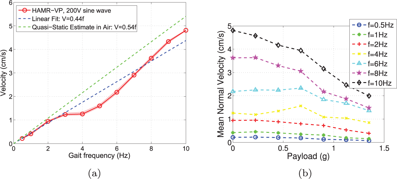
Power measurements for HAMR-VP. Trials were conducted from 1–50 Hz, recording power for all lift and drive actuators. There is negligible difference between measurements taken when robot is suspended and when it is walking across the ground as shown in the 150 V trials.

4.3. High speed locomotion

Running robots, constrained by actuator energy and bandwidth, typically use a biologically inspired approach to achieve high-speed dynamic gaits. By tuning compliant elements in their legs or transmissions, robots can exploit full-body dynamics to increase locomotion efficiency and induce aerial phases of locomotion, thus breaking kinematic constraints. Some of the world’s fastest robots have used tuned leg compliance to achieve speeds exceeding quasi-static maxima, notably: VelociRoACH (Haldane et al., 2013), Cheetah-cub (Spröwitz et al., 2013), DASH (Birkmeyer et al., 2009), Sprawlita (Cham et al., 2002), RHex (Saranli et al., 2001), and Boston Dynamics’s Cheetah Robot (Boston Dynamics, 2013). Elastic elements can additionally simplify gait control (Sponberg and Full, 2008), enhance obstacle avoidance (McNeill Alexander, 2002), and add shock absorption (Alexander, 1990); characteristics worth implementing into HAMR in the future. However, an alternative approach is taken in this work to increase locomotion speed above quasi-static performance by utilizing the high bandwidth and quality factor characteristics of the HAMR powertrain.

The HAMR powertrain benefits from efficient mechanical elements such as bending actuators and flexures with little energy loss due to friction or viscoelasticity. Furthermore, elastic elements in the powertrain (actuator and flexures) and low leg inertia result in high system resonances compared to other legged robots. The high powertrain bandwidth, along with actuator power that scales with frequency, enable the use of gait frequencies that exceed those used in some of the world’s fastest legged robots (RHex—5Hz, DASH—17Hz (Birkmeyer et al., 2009)). Additionally, a high quality factor leads to increased leg output amplitudes near powertrain resonance. Therefore, HAMR-VP’s powertrain dynamics were characterized and used to increase locomotion speeds and efficiency compared to quasi-static values in Section 4.2.

To exclude full-body dynamics from the discussion of locomotion near powertrain resonance, a simple experiment was performed to approximate full body resonance(s). The resonant frequency of a quadrupedal robot bouncing in the vertical plane, assuming an undamped oscillator similar to the spring-loaded inverted pendulum model, is $f_{n} = (1 / 2 π) \sqrt{k / m}$ , where m = 1.27 g is the robot mass and k is the combined linear spring stiffness of four parallel powertrains. The stiffness k was estimated by optically measuring robot sag height in response to incrementally adding weights to the back of the robot. The results are a nearly linear relationship between weight and sag height. A linear fit to the data yields a spring stiffness of k = 5.5 N/m, and resonant frequency f_n = 10.4 Hz. f_n represents the maximum body mode resonant frequency; with fewer legs on the ground k, and thus f_n, decrease. Assuming f_n ≤ 10.4 Hz, effects of body mode resonances will be ignored for the analysis near powertrain resonances (50–70 Hz) below. It may be constructive, however, to tune body resonance (as done in Altendorfer et al. (2001)) to enable dynamic locomotion. However, the body has multiple modes which change depending on constraints (i.e. how many legs on the ground) and some of these modes might be destructive to locomotion (e.g. hopping side to side). Finely tuning the robot’s dynamics would be necessary to mitigate these effects and can be ignored with a powertrain resonance much higher than body modes. Even without utilizing body dynamics, the mechanical elements of HAMR-VP’s powertrain allow high stride frequencies and amplitudes at resonance, resulting in high speed locomotion. The following sections describe this process.

4.3.1. Powertrain system identification

HAMR’s powertrain is a second order spring mass system, approximately linear for small leg angles. To characterize the system dynamics, all six robot DOFs (two drive and four lift) were actuated with the robot elevated from the ground at frequencies from 1–98 Hz. Sagittal plane outputs were recorded using a high-speed video camera (Phantom v7.3, Vision Research) at 100–3000 fps and measured using 2D motion tracking software (ProAnalyst, Xcitex). Drive and lift DOF amplitudes correspond to horizontal and vertical plane displacements, respectively.

The robot powertrain frequency responses were recorded using the nominal walking gait described in Figure 8; lift and drive DOFs of each leg were actuated 90° out of phase to generate a nominal circular trajectory. Input bias voltage and signal amplitudes were restricted to 100 V to prevent damage to the powertrains and prolong their lifetime. Figure 11 shows system Bode plots with amplitude normalized to the output at f = 1 Hz (assumed DC), and phase offset measured between input drive voltage and output displacement. Furthermore, displacement output of independently driven DOFs on HAMR-VP’s right side were recorded to identify coupling between lift and drive DOF (see Figure 12).

Figure 11.

Frequency response and second order damped oscillator model fits of HAMR-VP’s rear drive (a) and rear left lift (b) DOFs, driven using 100 V sinusoids and the nominal ψ_i values in Table 1. Similar results were obtained in the additional four DOFs, and system properties are summarized in Table 2.

Figure 12.

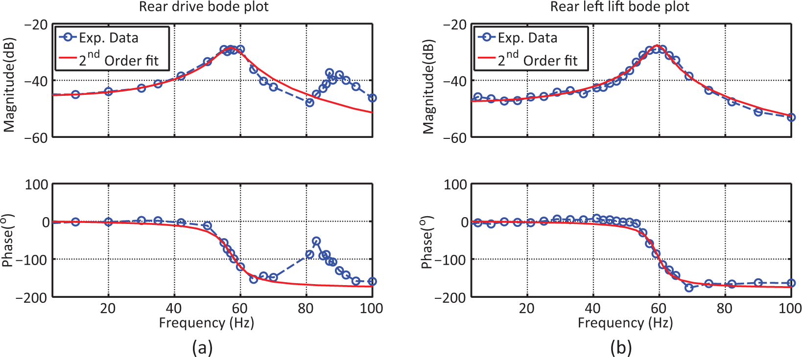
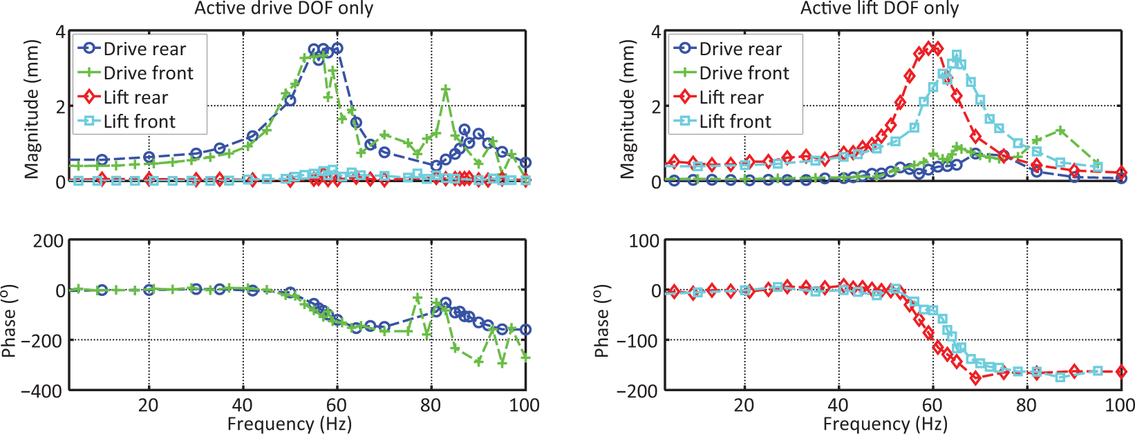
Frequency response of HAMR-VP’s right front (2) and right rear (4) legs with individual DOFs active. The response of passive DOFs when their orthogonal DOF is actuated (e.g. drive output in response to lift input) indicates that there is coupling near passive DOF resonant frequencies. The phenomenon is negligible for the lift DOF in response to drive, however substantial for drive in response to lift.

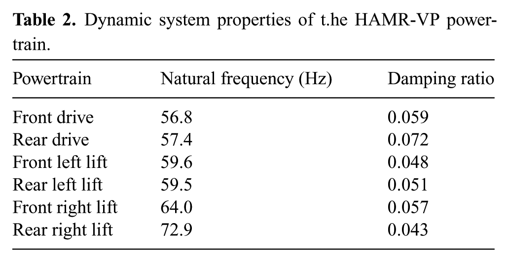
HAMR-VP’s powertrains resemble well-behaved linear time invariant second order systems with a high quality factor (Q = 4.1–7.9). Frequency response data can therefore be fit to a damped harmonic oscillator model of the form $\ddot{x} + 2 ζ ω_{0} \dot{x} + ω_{0}^{2} x = 0$ where x is a single DOF displacement output, ω₀ is the system natural frequency, and ζ is damping ratio. The system properties of each powertrain obtained from fit models using MATLAB’s fitfrd function (MathWorks, 2012a) are summarized in Table 2. Results indicate that all six powertrains are under-damped with damping ratio ζ between 0.043 and 0.072. Above powertrain resonance, output amplitudes attenuate below DC values, and phase shifts approach − 180°. There is a second resonant frequency in the drive DOF shown in Figure 11(a) near 90 Hz which is likely due to the coupling between the left and right side drive DOF. Another observation is the consistency of powertrain dynamic properties of Table 2, which simplifies control in Section 4.3.2.

Table 2.

Dynamic system properties of t.he HAMR-VP powertrain.

Powertrain	Natural frequency (Hz)	Damping ratio
Front drive	56.8	0.059
Rear drive	57.4	0.072
Front left lift	59.6	0.048
Rear left lift	59.5	0.051
Front right lift	64.0	0.057
Rear right lift	72.9	0.043

After examining the output of a passive DOF to its driven orthogonal DOF (i.e. actuate lift and measure drive amplitude) it is clear that there is minimal coupling between the lift DOF upon actuating the drive DOF. Actuating the lift DOF, however, results in coupling with the drive DOF between the two drive DOF resonant peaks. The second drive DOF resonant peak is ignored for this work, and locomotion in Section 4.3.3 is only performed using gait frequencies up to 75 Hz.

4.3.2. Tuning leg trajectory

Actuating the robot near powertrain resonance amplifies outputs above the low frequency values, which in theory increases locomotion efficiency by minimizing wasted reactive power. However, simply driving near powertrain resonant frequencies causes undesirable behavior due to output phase shifts. Using experimental data in the Bode plots in Figure 11 and their second order fits, appropriate walking trajectories can be generated. Figure 13 demonstrates the use of second order model fits to effectively apply a phase shift, α, to actuator input signals, creating elliptical foot trajectories. While tuning the leg inputs in air does not guarantee an optimal gait on the ground, the tuned input is used as an improved nominal gait pattern. Various effects of the foot–ground interaction such as the terrain, contact surface area, impact mechanics, and friction can all affect locomotion performance. Further studies on these foot–ground interactions are needed to evaluate these effects. In this work, tuning the leg inputs in air is used to generate an improved nominal gait pattern that enables high speed locomotion in Section 4.3.3.

Figure 13.

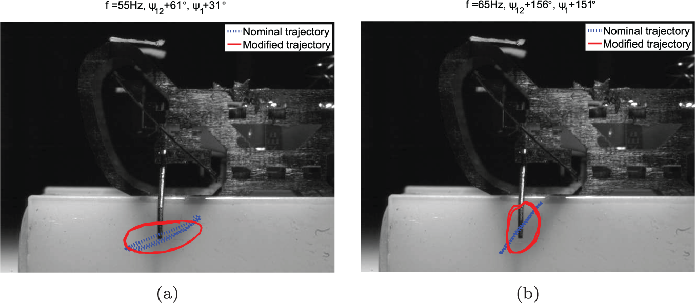
Actuation near powertrain resonant frequencies is susceptible to phase shifts characteristic of a second order linear system. Using the second order system models fit to powertrain frequency response data in Figure 11, appropriate phase shifts were applied to input sinusoidal voltages to generate elliptical leg trajectories. Here, results representative of the input tuning process are shown for unmodified and modified outputs of HAMR-VP’s front left leg near drive (a) and lift (b) resonances (55 Hz and 65 Hz, respectively). Tuned phases are α_Li = 31°, α_Dr = 61° and α_Li = 151°, α_Dr = 156° at 55 Hz and 65 Hz, respectively.

4.3.3. Dynamic regime locomotion results

Using the powertrain system identification from Section 4.3.1, HAMR-VP was capable of locomotion above the base quasi-static regime in Section 4.2 (1–10Hz). In this section, the robot is nominally fed inputs to generate circular leg trajectories and a trot gait defined in Figure 8. The walking surface is card stock and data is collected using high-speed videography (Phantom v7.3, Vision Research). Carbon fiber legs were used for all high speed locomotion trials. Using intuition gained in Section 4.3, full body dynamics are ignored, assuming the maximum system resonance is 10.4 Hz.

In initial trials, HAMR-VP’s speed ceased to increase with frequency above 10 Hz; locomotion was characterized by the robot bouncing off of the ground in the vertical direction, slowing or preventing forward motion. Examining the powertrain frequency response data in Figure 11 and high speed video of the robot’s sagittal plane during locomotion provides an explanation. Above 10 Hz, powertrain output amplitude begins to increase with frequency, and enough lift DOF force is generated to propel the robot off of the ground. When feet leave the ground asymmetrically, one or more strides are missed, altering speed and trajectory. Two solutions exist to this problem: increasing mass or decreasing lift input amplitude; the latter, more energy efficient approach was taken here.

Above 40 Hz gait frequency, in addition to increasing output amplitude, phase shifts caused undesirable leg outputs that altered the direction of locomotion. Using the tuning strategy developed in Section 4.3.2, input phases were adjusted with a constant phase offset α dictated by second order system fits. From 40–75 Hz, leg inputs were tuned to enable HAMR-VP to take advantage of its high quality factor powertrain dynamics. Because of the relatively low variance between each leg’s frequency response, a single lift phase and single drive phase offset were chosen for these trials, using leg 1 as the basis. The resulting locomotion was biased to the left, however straight enough to traverse a 17cm × 17cm track without collisions.

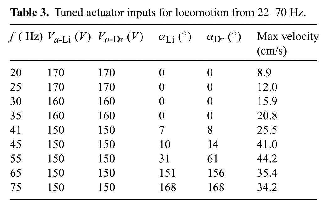
Speed results at selected gait frequencies with tuned inputs (summarized in Table 3) are shown in Figure 14. Velocities at gait frequencies above 20 Hz are plotted coincident to quasi-static results from Section 4.2, which shows that HAMR-VP transitions to a regime where projected quasi-static maximum velocities are exceeded for gait frequencies of 40–55 Hz. The mechanism enabling greater than quasi-static speeds is inconclusive; however it is likely a combination of increased stride amplitudes as dynamics approach resonance, and aerial phases that eliminate quasi-static speed constraints. These results are similar to those seen in biological locomotion where running speed increases linearly with stride frequency during walking and trotting gaits until transition to a galloping gait where speed becomes independent of stride frequency (Ting et al., 1994; Blickhan et al., 1993). For HAMR-VP, operation beyond 55 Hz results in a decrease in speed, which implies an optimal gait frequency for minimum cost of transport. The maximum speed that HAMR-VP reached in these trials was 44.2 cm/s (10.1 body lengths per second) and consistently ran at velocities above 25 cm/s from 45–75 Hz actuator frequencies. See Figure 15 for representative frames captured during high speed locomotion.

Table 3.

Tuned actuator inputs for locomotion from 22–70 Hz.

f (Hz)	V_a_-Li (V)	V_a_-Dr (V)	α_Li (°)	α_Dr (°)	Max velocity (cm/s)
20	170	170	0	0	8.9
25	170	170	0	0	12.0
30	160	160	0	0	15.9
35	160	160	0	0	20.8
41	150	150	7	8	25.5
45	150	150	10	14	41.0
55	150	150	31	61	44.2
65	150	150	151	156	35.4
75	150	150	168	168	34.2

Figure 14.

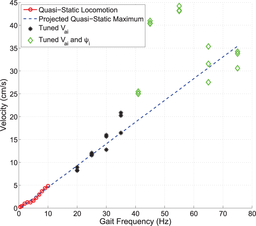
High speed locomotion above the 1–10 Hz quasi-static regime of the HAMR-VP robot was enabled by tuning actuator inputs using the powertrain frequency response data in Section 4.3.1. At gait frequencies from 20–35 Hz, lift DOF voltage amplitudes were attenuated to prevent the robot from bouncing off of the ground, thus disrupting straight line locomotion. From 40–75 Hz, locomotion near powertrain resonances was enabled by attenuating and applying phase shifts to the input voltage (see Table 3). Velocities are plotted coincident to quasi-static results and their linear fit, which shows that between 40–55 Hz, speeds exceed the projected quasi-static maximum. Although results are inconclusive, this is likely due to a combination of increased stride amplitudes as dynamics approach resonance and airborne phases that remove speed constraints based on maximum stride length.

Figure 15.

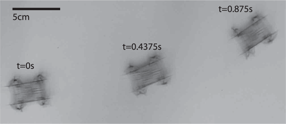
HAMR-VP reaches speeds up to 44.2 cm/s (10.1 body lengths per second) with a 55 Hz gait frequency.

Power. Total electrical power of the six HAMR-VP actuators was measured from 1–50 Hz at 150 V and up to 17 Hz at 100 V and 200 V. The data is shown in Figure 10. The power ranges from 5.6 mW at 100 V and 2 Hz to 52.5 mW at 200 V and 17 Hz. As indicated by the 150 V trials, the power increases linearly with frequency up to the tested maximum frequency of 50 Hz. There is negligible difference between the 150 V trials on the air and on the ground due to the low electromechanical coupling of the piezoelectric actuators.

Cost of transport. Cost of transport, defined as $C O T = \frac{Average Power}{Speed \times Mass}$ , is calculated with power measurements and speed data from Figure 14. A logarithmic plot of cost of transport vs. gait frequency is shown in Figure 16(a). Similar to biological data of cockroaches and crickets (Full et al., 1990), the cost of transport of HAMR-VP decreases with increasing speed. The minimum cost of transport for HAMR-VP is 109 J/m/kg at a gait frequency of 50 Hz (41.0 cm/s). Above 50 Hz, power estimates are extrapolated using a linear fit to the 150 V power data in Figure 10 (P = (0.82f + 13.0) mW). Using this fit and the speed data from Table 3, the cost of transport of HAMR-VP above 50 Hz gait frequencies is projected to increase as shown in Figure 16(a).

Figure 16.

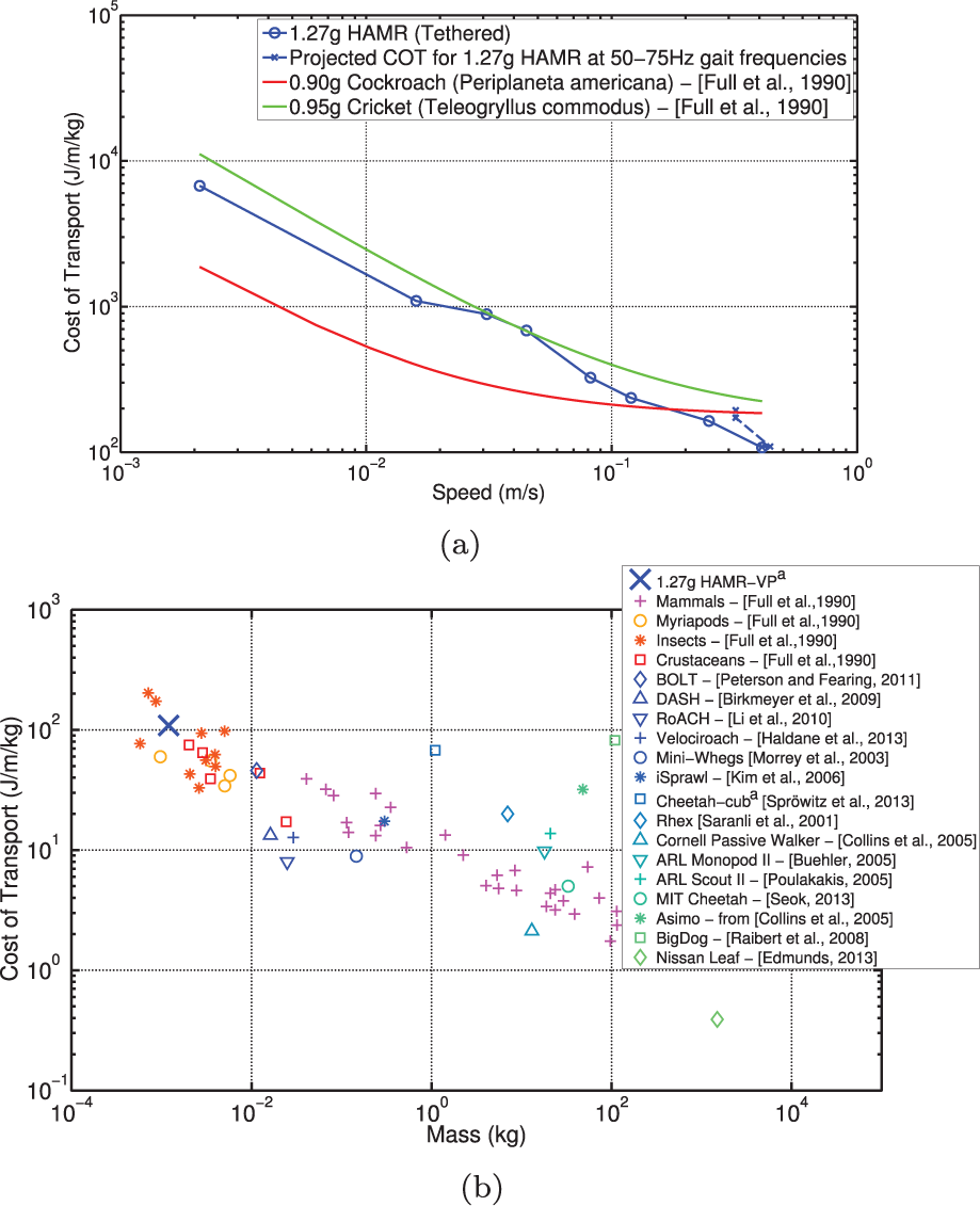
(a) Logarithmic plot of mass-specific energy per unit distance (cost of transport). Biological cost of transport data fits from Full et al. (1990) are overlaid with HAMR data. Cost of transport decreases with increasing speed in the biological data. Similarly, HAMR-VP’s COT decreases with increasing speed until the minimum COT of 109 J/m/kg at 50 Hz (41.0 cm/s). Beyond this gait frequency, HAMR-VP has a higher projected COT. (b) Logarithmic plot of minimum cost of transport vs. mass. HAMR-VP has a minimum cost of of 109 J/m/kg and is plotted among data collected from biology. The COT for similar mobile robots is presented for reference and comparison^b (Full et al., 1990; Saranli et al., 2001; Morrey et al., 2003; Buehler, 2005; Collins et al., 2005; Poulakakis et al., 2005; Kim et al., 2006; Raibert et al., 2008; Birkmeyer et al., 2009; Li et al., 2010; Peterson and Fearing, 2011; Edmunds, 2013; Haldane et al., 2013; Seok et al., 2013; ?).

In these measurements, HAMR is tethered to an off-board power supply. As described in Section 4.2.1, a small decrease in speed is expected with an added payload for battery and power electronics. Due to the low electromechanical coupling of the piezoelectric actuators, the power required by HAMR-VP is expected to remain the same regardless of payload. Therefore, the decrease in speed is expected to approximately offset the increase in mass at low speeds. The effect at high speeds (above 20 Hz) is more difficult to infer due to the unknown terrain, dynamic effects, and friction but it is likely that a more significant reduction in speed with added power electronics payload will result in an asymptotic approach to a minimum COT, similar to the biological data.

A logarithmic plot of minimum cost of transport vs. mass for combined robot and biological data is shown in Figure 16(b). The COT for mobile robots under 1 kg follows a similar trend as the biological data, although the COT for mobile robots over 1 kg varies quite a bit. HAMR-VP is the lightest robot in this category and has a COT similar in magnitude to the COT of myriapods and insects from Full et al. (1990).

5. Maneuverability and control

Insect-scale legged robots have the potential to locomote on rough terrain, crawl through confined spaces, and scale vertical and inverted surfaces. To navigate these environments, it is important for the robot to be able to control position and orientation in addition to the straight line, open-loop locomotion presented in the previous sections.

Similar to straight line locomotion dynamics, HAMR-VP has different maneuverability characteristics at low and high frequencies. Frequencies of 2 Hz and 40 Hz are chosen to represent the low and high speed maneuverability performance. These frequencies are chosen because 2 Hz is slow enough to track and feedback control via a USB camera and 40 Hz is fast but still far enough from the resonance so that straight locomotion is achieved without adjusting the phase.

High speed videos show that HAMR-VP’s turning characteristics are very different between low speed and high speed locomotion. For example, the robot’s tilt with respect to the sagittal plane is obvious at 2 Hz whereas at 40 Hz, the robot does not tilt at all. Additionally, there is a substantial difference in the forward speed of the robot between 2 and 40 Hz. The average lateral speed (crabbing speed), however, does not change between 2 and 40 Hz. This causes the crabbing motion to be apparent at low speeds, but negligible at high speeds. Figure 17 shows the comparison between normal and lateral speeds of the robot at low and high frequencyies. This behavior results in characteristics of a holonomic system at low speeds and a non-holonomic system at high speeds and therefore the two regimes need to be investigated as separate cases.

Figure 17.

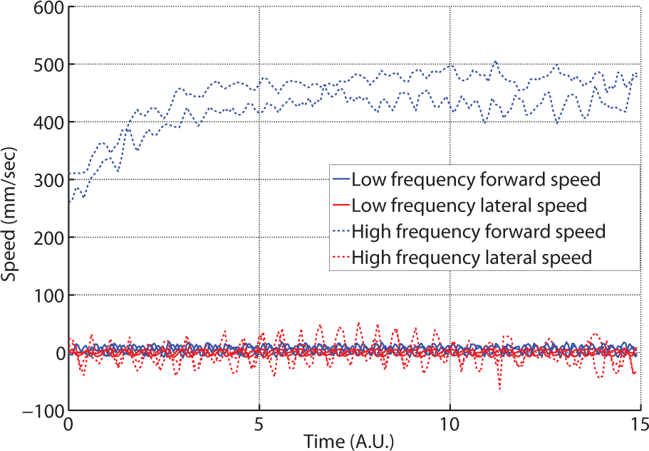
Comparison of forward (normal) speed and lateral (crabbing) speed of HAMR-VP between low and high frequencies. Two experiments are run at each frequency (2 Hz and 40 Hz). While the average forward and lateral velocity values are comparable at low frequency operation, the mean forward velocity is much higher than mean lateral velocity at high frequency operation. This behavior results in holonomic-like motion at low frequencies and non-holonomic-like motion at high frequencies. It also means that the lateral motion of the robot is negligible at high frequencies, hence it does not need to be controlled.

5.1. Feedforward parameter sweep

The parameters in Table 1 were explored to determine appropriate turning schemes for HAMR-VP in both the low speed and high speed locomotion regimes. The primary goal was to achieve control of body orientation in the walking plane (θ) with the simplest possible controller (i.e. fewest parameters). In general, turning is achieved by introducing asymmetry between the kinematics or frequency of left and right sides of the robot. However, HAMR-VP’s mechanical coupling of contralateral drive DOFs precludes the use of swing mechanics to generate asymmetry between the left and right legs using a single parameter. Therefore, the sagittal plane (lift) mechanics must be driven asymmetrically, contrary to the mechanics of turning in insects that primarily occurs in the walking plane (Jindrich and Full, 1999). Here, we investigate the following parameters to introduce asymmetries between the left and right side leg lift motions: phase (with respect to its drive actuator), duty cycle, and mean voltage of lift actuators.

5.1.1. Low speed maneuverability

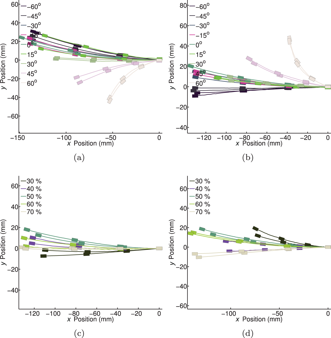
The results for varying the three parameters of interest independently on the left front lift actuator and right front lift actuator are shown in Figure 18. Bidirectional turning is observed when the phase of either leg lift is varied. For example, increasing the front left leg lift phase by 60° (with respect to the nominal phase) turns the robot to the right while decreasing the front left leg lift phase by 60° turns the robot to the left. The opposite occurs on the front right leg lift. Varying the duty cycle of a single lift actuator is less effective inducing turns than modifying the phase. Varying the peak-to-peak voltage does not cause turning.

Figure 18.

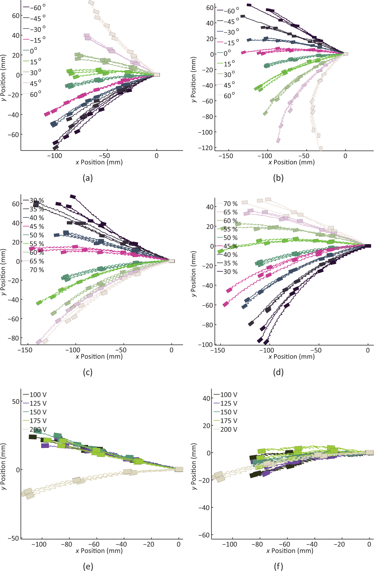
Low speed maneuverability using the phase (a and b), duty cycle (c and d), or mean voltage (e and f) parameters of a single lift actuator (left front lift or right front lift). Changing the lift phase of a single leg with respect to its swing turns the robot at low frequencies. Varying the duty cycle has a similar effect. It should also be noted that with changes in the duty cycle, the robot also moves laterally. The plots (e) and (f) show that mean voltage of lift actuators cannot be used for position control.

The effect of leg lift phase and duty cycle of the left and right sides of the robot are seen in Figure 19. Modifying the front and rear leg lift phases of a single side causes a tighter turning radius than modifying only a single leg. Modifying the duty cycle of front and rear legs of a single side primarily varies the lateral velocity (crabbing motion) of the robot. For example, when the duty cycle of both left side lift actuators is decreased to 30%, the robot will ‘crab’ to the right.

Figure 19.

Low speed maneuverability using the phase (a and b) and duty cycle (c and d) of two lift actuators (front and rear left lift or front and rear right lift). Changing the lift phase of two legs with respect to its swing causes the robot to turn at low frequencies. On the other hand, varying the duty cycle changes the robot’s lateral velocity without causing a significant change in forward velocity or orientation.

Varying the phase of all four lift actuators simultaneously results in the best heading control, allowing the robot to complete very tight turns. The lowest turning radius of the robot at low frequency operation is 14 mm. This data is shown in Figure 20.

Figure 20.

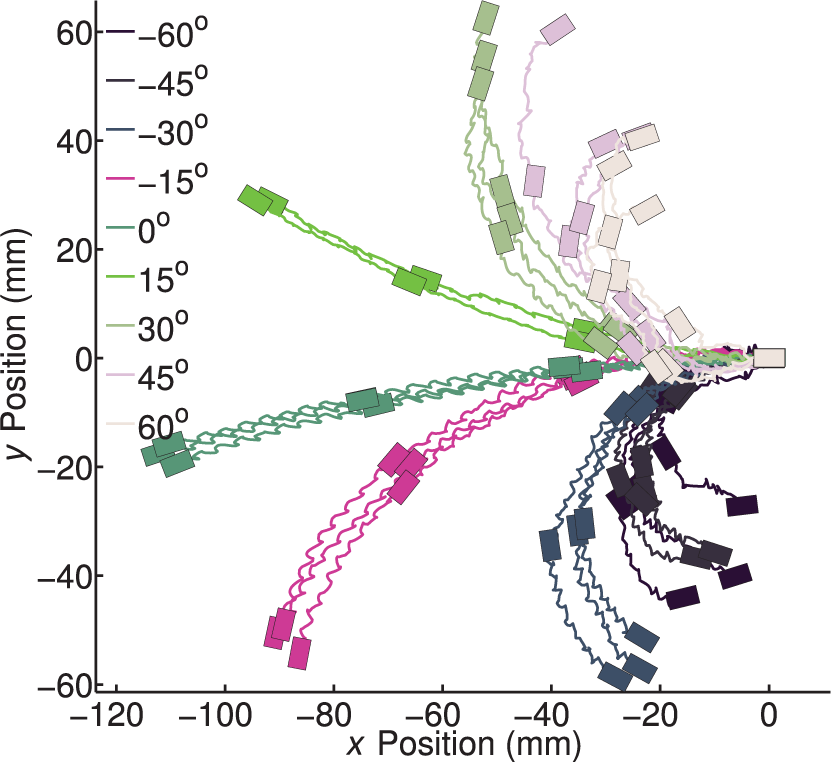
Low speed maneuverability using the phase of all four lift actuators. Varying all four phases with a single value causes the robot to turn. The robot can make very tight turns using this strategy.

5.1.2. High speed maneuverability

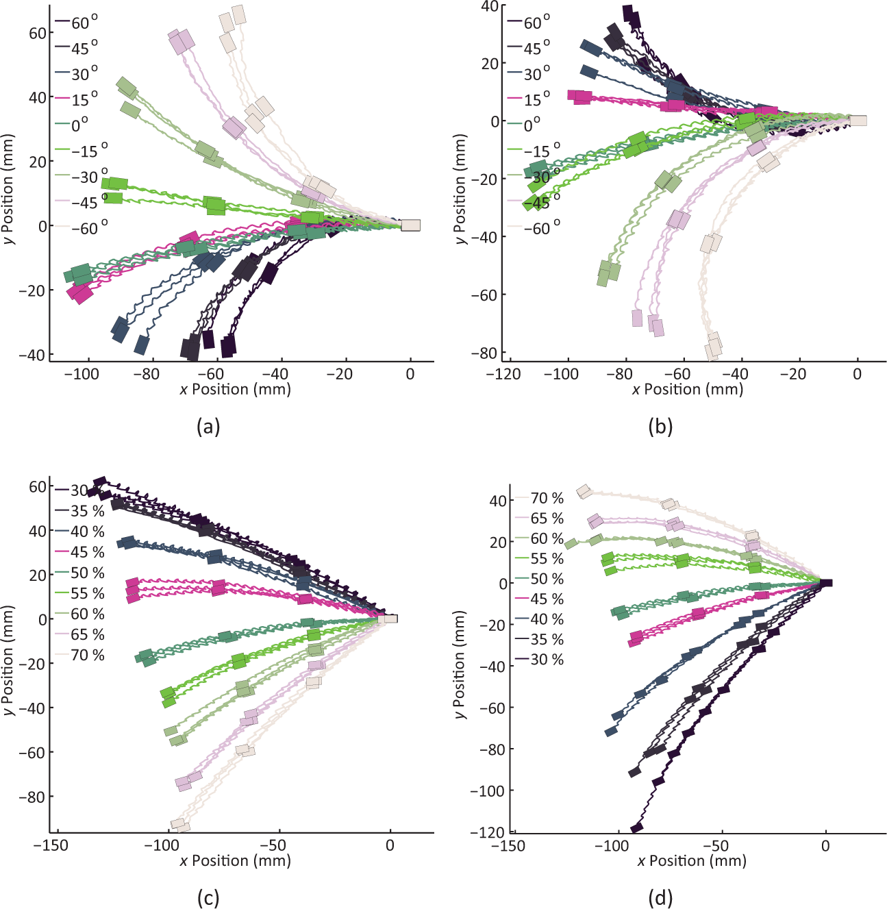
At high frequencies, lateral motions of HAMR-VP are less pronounced compared to low frequencies. Hence we only seek a parameter to control the heading. The results for varying the three parameters of interest independently on the left and right front lift actuators are shown in Figure 21.

Figure 21.

High speed maneuverability using the phase (a and b), duty cycle (c and d), or mean voltage (e and f) parameters of a single lift actuator (left front lift or right front lift). Changing the lift phase of a left/right leg with respect to its swing turns the robot left/right at low frequencies. Varying the duty cycle has a similar effect as well. We could not accomplish turning both directions using a single leg phase or duty cycle. The plots (e) and (f) shows that mean voltage of lift actuators cannot be used for position control as the behavior is not consistent.

Turning towards one side is observed when the phase of either leg lift is varied. For example, increasing the front left/right leg lift phase by 60° from nominal turns the robot to the left/right. This is the opposite behavior as seen in the low speed maneuverability. High speed videos show that the robot does not tilt with respect to the sagittal plane during 40 Hz locomotion compared to the large body tilts at 2 Hz. The lack of body tilt prevents the leg slipping seen at low speeds and causes the robot to maneuver differently at low and high speeds. At high speeds, the robot mainly turns due to a force difference between the left and right sides of the robot resulting in opposite turning directions from low speeds given the same phase offsets. At high speeds, the robot always turns towards the side with altered phase due to a decreased applied force on that side.

Varying the duty cycle of a single lift actuator causes a reduced degree of turning and varying the peak-to-peak voltage does not introduce turning.

The effect of leg lift phase and duty cycle of the left and right sides of the robot are seen in Figure 22. Modifying the front and rear leg lift phases of a single side results in tighter turns compared to modifying only a single leg. Unlike the low speed maneuverability, modifying the duty cycle of front and rear legs of a single side does not introduce turning or lateral motions.

Figure 22.

High speed maneuverability using the phase (a and b) and duty cycle (c and d) of two lift actuators (front and rear left lift or front and rear right lift). Similar behavior with single leg high speed experiments shown in Figure 21 are observed for phase experiments as the robot only turns towards the direction of the legs whose phases are modified. On the other hand, duty cycle modification did not cause consistent change in robot’s heading.

Lastly, similar to low speed maneuverability, varying the phase of all four lift actuators simultaneously results in the best heading control. The lowest turning radius achieved using this strategy is 87 mm. Again, the direction of the turn is in the opposite direction as seen in the low speed maneuverability (Figure 23). As previously mentioned, the opposite turning direction from low speed is not unusual due to the different turning mechanism; however, it is convenient that the same parameter works at both low and high frequencies because this makes the control structure easier.

Figure 23.

High speed maneuverability using the phase of all four lift actuators. Varying all four phases with a single value causes the robot to turn at high frequencies, similar to the low frequency results shown in Figure 20.

5.2. Control

Using the control inputs from Section 5.1.1, two simple feedback controllers are implemented to control the orientation and the lateral velocity of the robot.

5.2.1. Experimental setup

An experimental setup was built to implement a feedback controller. The low-level code responsible for generating the drive signal waveforms runs on an xPC target and is written in Matlab/Simulink. The host PC runs the high-level drive code and the user interface, both written in Matlab. A camera (PixeLINK, PL-B741F) is connected to the host PC via IEEE 1394 and interfaced with the high level Matlab code to provide position and orientation data. The architecture of the experimental setup is shown in Figure 24. In the current method of video tracking, the maximum frequency for the feedback controller is limited to 3 Hz; therefore, only low speed control experiments are conducted. However, on-board sensors that can replace camera feedback are currently being developed. These sensors will be implemented for future studies in order to provide faster sensor input and increase the speed of the control loop. The controller presented here is intended as a proof-of-concept demonstration that such a feedback controller is possible.

Figure 24.

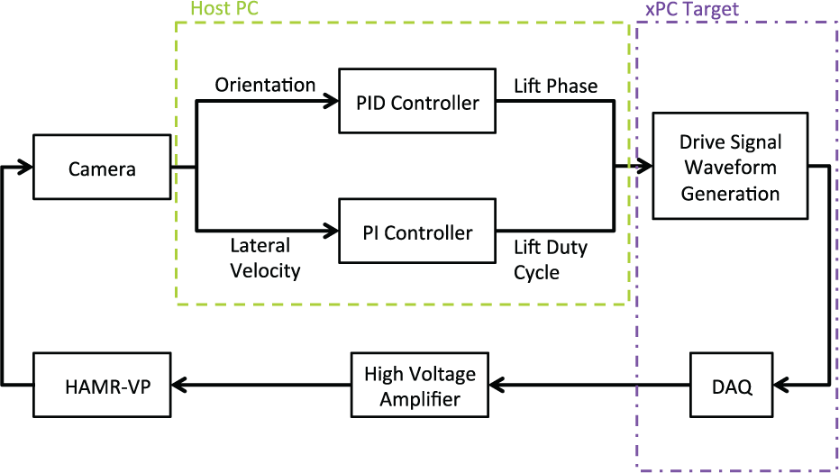
The architecture of the experimental setup. The host computer collects position and orientation of the robot through a camera and runs two feedback control loops. The outputs of the control loops are sent to the drive signal generation code running on the xPC target and are fed to the robot through a power amplifier.

Motion estimation code detects red markers on three corners of the robot frame, which are used to identify the center of mass and orientation. The center position and orientation data are then filtered using the robust local regression method (the ‘rlowess’ method in Matlab). After filtering the data, normal and lateral velocities with respect to the robot body are found by transforming global velocities to the robot’s coordinate frame.

As described in Section 5.1.1, modifying the lift phases of each leg can control robot’s orientation. A single PID loop is used to control the robot’s orientation. This control loop takes orientation data from the camera, filters the data as described above, finds the error between the desired orientation specified by the user and the actual robot orientation, and modifies the lift phase of all the legs. This loop runs on the host PC, and sends the new phase to the xPC target, which modifies the drive signal accordingly. The derivative of the error is found numerically using the error from current time step, the previous error, and the sampling time.

We also control the lateral velocity of the robot by modifying the duty cycle of the lift actuators as described in Section 5.1.1. A PI controller is implemented for lateral velocity control. This control loop takes the lateral velocity data, finds the error between the desired and actual speed, and modifies the lift duty cycle of the front and rear right legs. This loop also runs on the host PC and sends the modified duty cycle to the xPC target. The separation of orientation and lateral velocity controllers to different parameters enables the loops to run independent of each other.

5.2.2. Controller results

Using the method described in Section 5.2.1, an orientation controller (without lateral velocity control) is implemented. Due to the latency issues with Matlab’s computer vision toolbox, the control loop was able to run at a maximum frequency of 3 Hz; hence the robot is run with 2 Hz sinusoidal drive signals.

The PID gains of the orientation controller are manually tuned: 3, 0.2, and 0.15 (proportional, integral, and derivative) are found to perform well. Desired orientations of 0, 20, and −20 degrees are used as shown in Figure 25(a) and (b).

Figure 25.

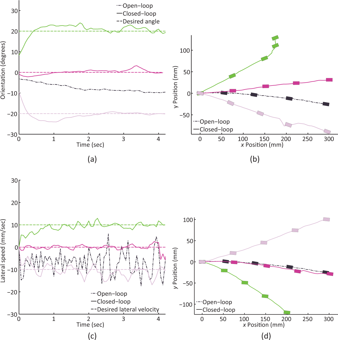
The results of the orientation control and lateral control experiments. (a) The dashed lines are desired orientations whereas the solid lines are actual orientation data acquired from the camera. The black dashed-dotted line shows the open-loop trial in which the robot’s orientation is not constant even with nominal drive parameters. (b) Even though the orientation of the robot is controlled, the non-zero lateral velocity of the robot prevents the controller from achieving perfect motion control. (c) The dashed lines are desired lateral velocities whereas the solid lines are actual lateral velocity data acquired from the camera. The black dashed-dotted line shows the open-loop trial in which the robot’s lateral velocity is increasing in time with the nominal drive parameters. (d) Similar to orientation control, the lateral controller is not sufficient to control the motion of the robot, since the robot’s orientation is not constant. The noise in the lateral speed measurements are caused by tilting of the robot’s body around its medial axis during stepping which is recorded by the camera.

The results in Figure 25(a) demonstrate that the controller is able to control the robot’s angle. It should be noted that small oscillations in the orientation data are caused by small changes in the observed marker positions from the stepping motion of the robot, not actual changes in the robot angle. Although the orientation controller works properly, Figure 25(b) shows that robot does not move along its medial axis (i.e. not straight forward). The robot exhibits a non-zero lateral velocity; hence, the orientation controller itself is not sufficient to control robot’s motion.

A lateral velocity controller is implemented and tested using a 2 Hz sinusoidal drive signal frequency. The PI gains are manually tuned to 0.3 (proportional) and 0.1 (integral). Desired lateral speeds of 10, 0 and −10 mm/sec are used. Results of these experiments are presented in Figure 25(c) and (d).

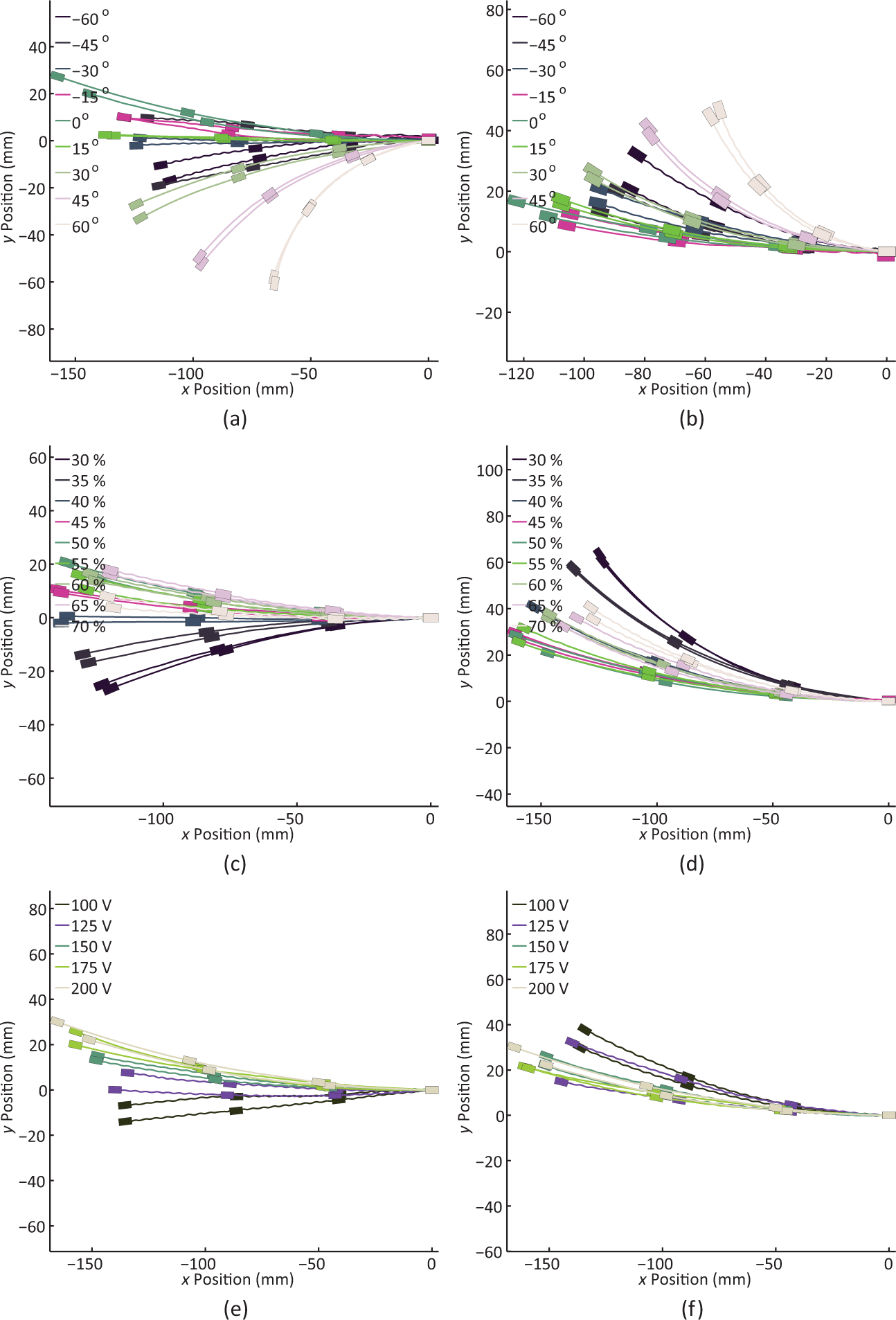
Similar to the orientation controller experiments, the lateral velocity controller is not sufficient to control robot’s motion since the orientation of the robot changes during the experiments. In order to control the robot motion and follow a desired trajectory, the orientation and lateral velocity controllers are used together without additional modifications. Desired trajectories are generated a priori. During operation, the controller finds the robot position, then finds the closest point on the desired trajectory and chooses the desired orientation as tangent to the desired trajectory at the closest point. It also chooses the desired lateral velocity to be along the line connecting the robot center of mass to the nearest point on the trajectory. The results of trajectory tracking experiments are shown in Figure 26.

Figure 26.

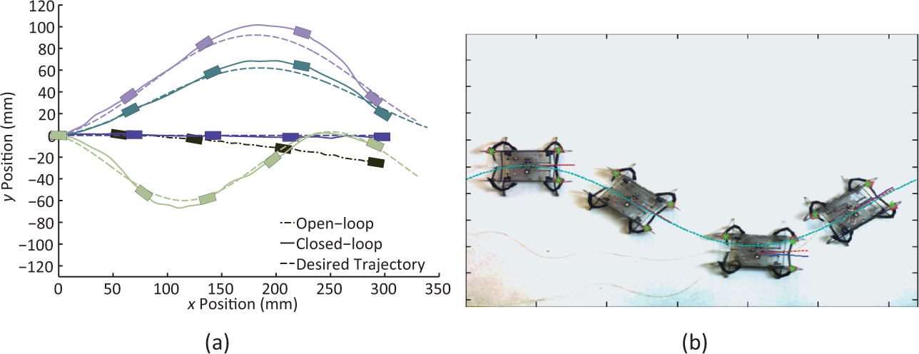
The results of the trajectory control experiments in which both control loops are running. (a) The black dashed-dotted line is the open-loop operation, the dashed lines are desired trajectories, and the solid lines are actual robot trajectories. The robot is able to follow a straight line (blue line) and sinusoidal trajectories. (b) Overlayed screen shots from a sinusoidal trajectory tracking experiment. The sinusoidal curve shown with light blue is the desired trajectory, the green stars are the marker locations, the red dashed line starting from the robot’s center is the instantaneous desired orientation and the blue line is the robot’s actual orientation. Each screen shot is 1.5s apart.

The results show that while the robot does not move straight during open-loop operation, the trajectory controller can enable HAMR-VP to walk straight or follow trajectories. HAMR-VP has a minimum turning radius of 14 mm and maximum lateral to forward velocity ratio of 0.4, which are the limits of its maneuverability. The minimum turning radius and the maximum lateral to forward velocity ratio reported are obtained from the experiments in Section 5.1.1, and are the values obtained using only the parameters selected as the possible control parameter candidates. As shown in Figure 26(a), the robot follows the straight and sinusoidal trajectories (radius of curvature = 44 mm, 66 mm, and 29 mm from top to bottom in Figure 26(a)) successfully, with some difficulty at the lowest radius of curvature (light purple line). Even though the robot cannot track steep trajectories, it manages to gradually decrease the position and orientation error after the turns by pushing itself towards the trajectory using the lateral velocity controller.

The trajectory controller includes only two filters and two feedback control loops and all the computation is done numerically. Therefore, the trajectory controller is computationally light (the required RAM is 44 bytes) and can be implemented on an ATmega 168 Atmel processor, for example. While increasing speed of motion capture is out of the scope of this work, feedback from a nine-axis accelerometer, gyroscope, and magnetometer (e.g. MPU-9150 from Invensense) will replace the information from the camera to form the feedback loop on orientation and the lateral velocity, enabling feedback control at higher speeds.

6. Conclusion and future work

We have presented the design of HAMR-VP, a 1.27 g quadrupedal microrobot manufactured using the PC-MEMS fabrication paradigm and pop-up assembly techniques. The main contributions of this work are in robot design for pop-up assembly, demonstration of high speed locomotion, and trajectory control in an insect-sized robot. This robot, along with related structures and mechanisms (Whitney et al., 2011; Sreetharan et al., 2012), demonstrate a variety of complex miniature devices achievable only by implementing pop-up assembly into PC-MEMS manufactured devices. While most robots decrease their complexity as size is reduced, pop-up MEMS devices allow for greater complexity given the range of mechanisms/DOFs available. This increased complexity allows many more gait and control parameters for HAMR-VP that would otherwise be unavailable in a robot at this scale.

HAMR-VP demonstrates locomotion performance that parallels locomotion in biology. HAMR-VP reaches speeds up to 44.2 cm/s (10.1 body lengths per second), has a minimum cost of transport of 109 J/m/kg, and can carry a payload of 1.35 g (106% of body mass). HAMR-VP is maneuverable at low and high speeds with minimum turning radii of 14 mm and 87 mm, respectively, and is able to follow trajectories at low speeds using offboard position and orientation feedback.

The demonstration of these capabilities in an insect-sized robot enables HAMR-VP to be a platform for future research on microrobots and bio-inspired terramechanics. Future work includes implementation of onboard electronics similar to HAMR3 (Baisch et al., 2011) and feedback control using onboard sensing. Locomotion on new terrains as well as varying leg and foot designs will be evaluated to explore the effect of foot–ground interactions on the dynamic locomotion of the robot. Another future topic includes developing an analytical model to understand the role of each design parameter and further optimize locomotive performance.

Footnotes

Acknowledgements

The authors would like to thank all Harvard Microrobotics Laboratory group members for their invaluable discussions.

Funding

This work was supported by the Wyss Institute for Biologically Inspired Engineering and the Army Research Labs Micro Autonomous Systems and Technology Program (grant W911NF-08-2-0004).

References

Alexander

(1990) Three uses for springs in legged locomotion. The International Journal of Robotics Research 9(2): 53–61.

Altendorfer

Moore

Komsuoglu

. (2001) Rhex: A biologically inspired hexapod runner. Autonomous Robots 11(3): 207–213.

Baisch

Heimlich

Karpelson

. (2011) HAMR3: An autonomous 1.7 g ambulatory robot. In: Proceedings of IEEE/RSJ International conference on intelligent robots and systems, San Francisco, CA, USA, 25–30 September 2011, pp. 5073–5079.

Baisch

Sreetharan

Wood

(2010) Biologically-inspired locomotion of a 2 g hexapod robot. In: Proceedings of IEEE/RSJ International conference on intelligent robots and systems, Taipei, Taiwan, 18–22 October 2010, pp. 5360–5365.

Baisch

Wood

(2011) Design and fabrication of the Harvard ambulatory micro-robot. In: Robotics Research. Berlin: Springer, pp. 715–730.

Birkmeyer

Peterson

Fearing

(2009) Dash: A dynamic 16 g hexapedal robot. In: Proceedings of IEEE/RSJ International conference on intelligent robots and systems, St Louis, MO, USA, 11–15 October 2009, pp. 2683–2689.

Blickhan

Full

Ting

(1993) Exoskeletal strain: Evidence for a trot-gallop transition in rapidly running ghost crabs. Journal of Experimental Biology 179(1): 301–321.

BostonDynamics (2013) CHEETAH—Fastest Legged Robot. Available at: http://www.bostondynamics.com/robot_cheetah.html.

Buehler

(2005) Dynamic locomotion with one, four and six-legged robots. Technical report, DTIC Document.

10.

Cham

Bailey

Clark

. (2002) Fast and robust: Hexapedal robots via shape deposition manufacturing. The International Journal of Robotics Research 21(10–11): 869–882.

11.

Collins

Ruina

Tedrake

. (2005) Efficient bipedal robots based on passive–dynamic walkers. Science 307(5712): 1082–1085.

12.

Edmunds (2013) 2013 Nissan Leaf S 4DR hatchback electric 1-speed direct drive features and specs. Available at: http://www.edmunds.com/nissan/leaf/2013/features-specs.html?style=&sub=.

13.

Full

Koditschek

(1999) Templates and anchors: Neuromechanical hypotheses of legged locomotion on land. Journal of Experimental Biology 202(23): 3325–3332.

14.

Full

Kubow

Schmitt

. (2002) Quantifying dynamic stability and maneuverability in legged locomotion. Integrative and comparative biology 42(1): 149–157.

15.

Full

(1991) Mechanics of a rapid running insect: Two-, four- and six-legged locomotion. Journal of Experimental Biology 156(1): 215–231.

16.

Full

Zuccarello

Tullis

(1990) Effect of variation in form on the cost of terrestrial locomotion. Journal of Experimental Biology 150(1): 233–246.

17.

Goldman

Chen

Dudek

. (2006) Dynamics of rapid vertical climbing in cockroaches reveals a template. Journal of Experimental Biology 209(15): 2990–3000.

18.

Haldane

Peterson

Bermudez

FLG

. (2013) Animal-inspired design and aerodynamic stabilization of a hexapedal millirobot. In: Proceedings of IEEE International conference on robotics and automation, Karlsruhe, Germany, 6–10 May 2013, pp. 3279–3286.

19.

Hoffman

Wood

(2012) Turning gaits and optimal undulatory gaits for a modular centipede-inspired millirobot. In: 4th IEEE RAS/EMBS conference on biomedical robotics and biomechatronics (BioRob), Rome, Italy, 24–27 June 2012, pp. 1052–1059.

20.

Hollar

Flynn

Bellew

Pister

(2003) Solar powered 10 mg silicon robot. In: Proceedings of IEEE 16th annual International conference on micro electro mechanical systems (MEMS-03), Kyoto, Japan, 23 January 2003, pp. 706–711.

21.

Hoover

Steltz

Fearing

(2008) RoACH: An autonomous 2.4 g crawling hexapod robot. In: Proceedings of IEEE/RSJ International conference on intelligent robots and systems, Nice, France, 22–26 September 2008, pp. 22–26.

22.

Hudson

Corr

Payne-Davis

. (2011) Functional anatomy of the cheetah (acinonyx jubatus) hindlimb. Journal of Anatomy 218(4): 363–374.

23.

Jindrich

Full

(1999) Many-legged maneuverability: Dynamics of turning in hexapods. Journal of Experimental Biology 202(12): 1603–1623.

24.

Karpelson

Wei

Wood

(2012) Driving high voltage piezoelectric actuators in microrobotic applications. Sensors and Actuators A: Physical 176: 78–89.

25.

Kim

Clark

Cutkosky

(2006) isprawl: Design and tuning for high-speed autonomous open-loop running. The International Journal of Robotics Research 25(9): 903–912.

26.

Hoover

Birkmeyer

. (2010) Systematic study of the performance of small robots on controlled laboratory substrates. In: Proceedings of SPIE, Volume 7679, Orlando, FL, USA, 5 April 2010, p. 76790Z.

27.

McNeill Alexander

(2002) Tendon elasticity and muscle function. Comparative Biochemistry and Physiology—Part A: Molecular and Integrative Physiology 133(4): 1001–1011.

28.

Morrey

Lambrecht

Horchler

. (2003) Highly mobile and robust small quadruped robots. In: Proceedings of IEEE/RSJ International conference on intelligent robots and systems, Volume 1, Las Vegas, NV, USA, 27 October–1 November 2003, pp. 82–87.

29.

Murphy

Kute

Mengüç

. (2011) Waalbot II: Adhesion recovery and improved performance of a climbing robot using fibrillar adhesives. The International Journal of Robotics Research 30(1): 118–133.

30.

Ozcan

Baisch

Ithier

. (2014) Powertrain selection for a biologically-inspired miniature quadruped robot. In: Proceedings of IEEE International conference on robotics and automation, Hong Kong, China, 31 May–7 June 2014, under review.

31.

Peterson

Fearing

(2011) Experimental dynamics of wing assisted running for a bipedal ornithopter. In: Proceedings of IEEE/RSJ International conference on intelligent robots and systems, San Francisco, CA, USA, 25–30 September 2011, pp. 5080–5086.

32.

Poulakakis

Smith

Buehler

(2005) Modeling and experiments of untethered quadrupedal running with a bounding gait: The scout II robot. The International Journal of Robotics Research 24(4): 239–256.

33.

Pullin

Kohut

Zarrouk

. (2012) Dynamic turning of 13 cm robot comparing tail and differential drive. In: Proceedings of IEEE International conference on robotics and automation, St Paul, MN, USA, 14–18 May 2012, pp. 5086–5093.

34.

Raibert

Blankespoor

Nelson

. (2008) Bigdog, the rough-terrain quadruped robot. In: Proceedings of the 17th IFAC world congress, Seoul, South Korea, 6–11 June 2008, pp. 10823–10825.

35.

Raibert

(1985) Legged Robots that Balance. Cambridge, MA: The MIT Press.

36.

Saranli

Buehler

Koditschek

(2001) Rhex: A simple and highly mobile hexapod robot. The International Journal of Robotics Research 20(7): 616–631.

37.

Seok

Wang

Chuah

. (2013) Design principles for highly efficient quadrupeds and implementation on the MIT cheetah robot. In: Proceedings of IEEE International conference on robotics and automation, Karlsruhe, Germany, 6–10 May 2013, pp. 3307–3312.

38.

Sponberg

Full

(2008) Neuromechanical response of musculo-skeletal structures in cockroaches during rapid running on rough terrain. Journal of Experimental Biology 211(3): 433–446.

39.

Spröwitz

Tuleu

Vespignani

. (2013) Towards dynamic trot gait locomotion: design, control, and experiments with cheetah-cub, a compliant quadruped robot. The International Journal of Robotics Research 32(8): 932–950.

40.

Sreetharan

Whitney

Strauss

. (2012) Monolithic fabrication of millimeter-scale machines. Journal of Micromechanics and Microengineering 22(5): 055027.

41.

Teoh

Wood

(2013) A flapping-wing microrobot with a differential angle-of-attack mechanism. In: Proceedings of IEEE International conference on robotics and automation. Karlsruhe, Germany, 6–10 May 2013, pp. 1381–1388.

42.

Ting

Blickhan

Full

(1994) Dynamic and static stability in hexapedal runners. Journal of Experimental Biology 197(1): 251–269.

43.

Trimmer

WSN

(1989) Microrobots and Micromechanical Systems. Sensors and Actuators 19: 267–287.

44.

Whitney

Sreetharan

. (2011) Pop-up book MEMS. Journal of Micromechanics and Microengineering 21(11): 115021.

45.

Wood

Steltz

Fearing

(2005) Optimal energy density piezoelectric bending actuators. Sensors and Actuators A: Physical 119(2): 476–488.