
Abstract
Robotic motion planning algorithms for manipulation of deformable objects, such as in medical robotics applications, rely on accurate estimations of object deformations that occur during manipulation. An estimation of the tissue response (for off-line planning or real-time on-line re-planning), in turn, requires knowledge of both object constitutive parameters and boundary constraints. In this paper, a novel algorithm for estimating boundary constraints of deformable objects from robotic manipulation data is presented. The proposed algorithm uses tissue deformation data collected with a vision system, and employs a multi-stage hill climbing procedure to estimate the boundary constraints of the object. An active exploration technique, which uses an information maximization approach, is also proposed to extend the identification algorithm. The effects of uncertainties on the proposed methods are analyzed in simulation. The results of experimental evaluation of the methods are also presented.
1. Introduction
Planners for robotic manipulation of deformable objects, such as for intelligent robotic surgical assistants (e.g. Patil and Alterovitz, 2010), for robotic assembly of elastic materials (e.g. Cai et al., 1996), for manufacturing of textiles (e.g. Miller et al., 2011), or for automated food handling, require the ability to estimate the mechanical deformations of the objects that occur during the manipulation task. Estimation of the tissue response, in turn, requires knowledge of both object constitutive parameters and boundary constraints.
In this paper, novel algorithms for estimation and active exploration of boundary constraints of deformable objects from robotic manipulation data are presented. The proposed boundary constraint estimation algorithm is inspired by the occupancy grip mapping algorithms widely used in mobile robotics. It uses tissue deformation data collected with a stereo vision system, and employs a multi-stage hill climbing procedure to estimate the boundary constraints of the object. The proposed active exploration algorithm builds on a probabilistic formulation of the estimation algorithm, and employs an entropy minimization approach.
Exploration of an object through robotic manipulation is not a new research topic. For example, Maekawa et al. (1995) integrated tactile sensing and dexterous manipulation to explore an unknown object by a multi-fingered robot hand. Bicchi et al. (1999) presented an algorithm for simultaneously modeling and manipulating unknown objects using a dexterous gripper. Okamura and Cutkosky (2001) presented an algorithm for extracting the surface features of objects with different surface profiles using robotic fingers. Recently, Petrovskaya and Khatib (2011) proposed tactile object exploration for rigid objects. Studies on rigid object recognition via haptic information were proposed earlier (e.g. Gorges et al., 2010; Bekiroglu et al., 2011).
There is a substantial body of literature on estimation of constitutive parameters of deformable objects, such as biological tissue. Studies on estimation of tissue mechanical parameters commonly rely on specialized apparatus (e.g. Brouwer et al., 2001; Ottensmeyer, 2001; Kauer et al., 2002), motions, or procedures, including uniaxial loading (Mehrabian and Samani, 2009), indentations (Lang et al., 2002; Sangpradit et al., 2009, 2011; Bickel et al., 2009; Fong, 2009; Frank et al., 2010; Tsukune et al., 2012) and geometric tension, compression, and shear tests (Kerdok et al., 2003; Gao et al., 2010). In a recent study, Bickel et al. (2009) proposed a scheme which used movements of multiple points marked on the surface of the tissue as observed through magnetic resonance imaging to fit non-linear material models, unlike earlier studies in the literature that rely on collocated force-displacement measurements (e.g. D’Aulignac et al., 1999; Sangpradit et al., 2009; Jordan et al., 2011). Recent studies on needle insertion show the possibility to steer a needle tip to a designated position in a deformable biological tissue (Chentanez et al., 2009; Patil et al., 2011; Kobayashi et al., 2012).
Recently, Boonvisut and Çavuşoğlu (2012) and Boonvisut et al. (2012) proposed a parameter estimation scheme based on an inverse finite element method (FEM) that used data from common surgical manipulation movements (e.g. retraction or folding of tissue by a gripper). Yoshimoto et al. (2011) focused on shaping a deformable object so as to move fiducials into designed positions. Shibata et al. (2009) proposed a method for manipulation of a deformable object such as fabrics. Goldman et al. (2013) proposed a cycloidal pattern motion to explore and estimate compliance environments. Bhattacharjee et al. (2012) proposed a method to classify and recognize various objects including deformable objects such as a plush toy, a rug and a sponge. Drimus et al. (2012) classified rigid and deformable objects using a palpation procedure. Willimon et al. (2013) proposed an algorithm to estimate deformable surfaces without features.
As it will be formally defined in Section 2, this paper focuses on the class of problems where the robotic system tries to identify the boundary constraints of a deformable object, an unknown subset of a deformable object’s boundary that is assumed to be fixed (i.e. rigidly anchored) in space, through robotic manipulation.
To the best of the authors’ knowledge, there are no prior studies in the literature that specifically focused on estimation of boundary constraints of deformable objects during manipulation.
The rest of the paper is organized as follows. The formulation of the boundary constraint estimation problem is presented in Section 2. The proposed boundary constraint estimation algorithm is presented in Section 3, and the proposed active exploration algorithm is presented in Section 4. Simulation and hardware experiments for validation of the boundary constraint estimation algorithm are presented in Sections 5 and 6, respectively. The simulation and physical experiments for validation of the active exploration algorithm are presented in Sections 7 and 8, respectively. Discussion and conclusions are presented in Section 9.
2. Problem formulation
In this paper, we consider a single deformable body,
In the boundary constraint identification problem, the goal is to identify the unknown sets
Instead of dealing with a continuous representation, we will assume that there is a mesh representation of the surface,
One important issue is the complexity of the problem. If the surface mesh has N nodes, the number of possible outcomes is 2
N
. Also, most of these outcomes are not necessarily distinguishable. For example, the state of a node surrounded by several anchored nodes would not be easily observable. In order to address these problems, we will group adjacent nodes into P patches, where P < N. The states of the patches will be denoted by the variable
In the text, we will describe the boundary configurations by providing the set of anchored patches, for notational simplicity. For example, we will use {1 2} to indicate the boundary configuration
Finally, we will also assume that there is an approximate model of the body’s deformation available, which can be used to estimate the trajectories of the fiducials for a given set of boundary constraint states and the known end effector motion. Here, we will use finite element models (FEMs) of the deformable object as the underlying model. The trajectories of the fiducials estimated with the model will be denoted by yest(t,
3. Tissue boundary constraint identification with hill climbing algorithm
The boundary identification problem has similarities to the occupancy grid mapping problem in mobile robotics. In occupancy grid mapping, the map is discretized into small binary cells represented as an occupancy grid (Moravec and Elfes, 1985), and the mapping problem is reduced to identifying the states of each of the grid cell from available sensory information. Algorithms, such as the MAP algorithm (Thrun, 2003), successfully use a hill climbing approach (McLachlan and Krishnan, 1996) to efficiently estimate occupancy grid maps from noisy and uncertain measurements by maximizing the posterior expectations.
In this paper, we will pursue an approach inspired by the hill climbing based expectation maximization algorithms as presented below.
3.1. The basic hill climbing algorithm
The basic hill climbing algorithm proposed for estimation of object boundary constraints is given in Algorithm 1.
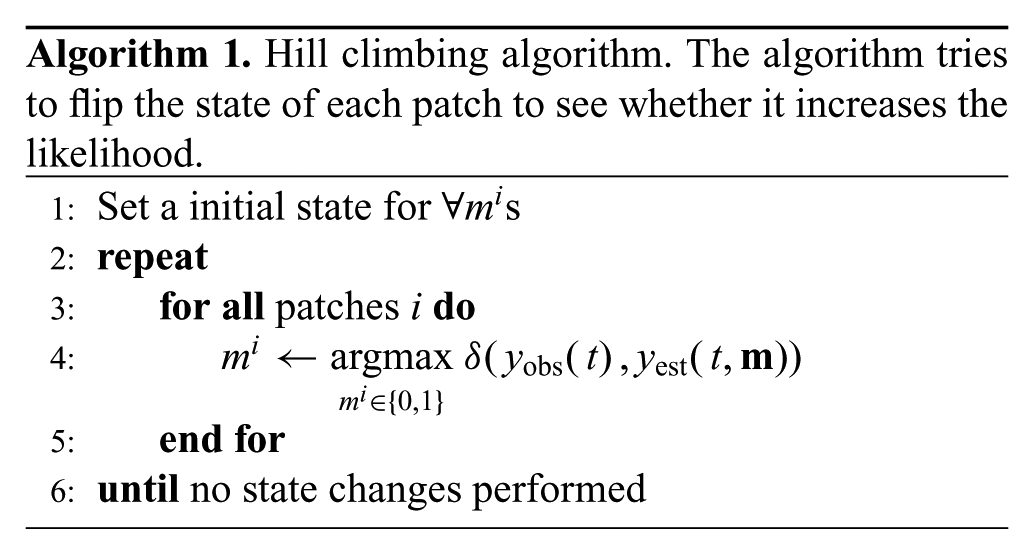
In this algorithm, the function δ(yobs(t), yest(t,
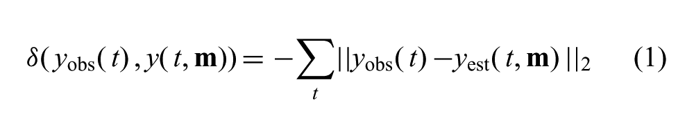
which has the same role as the posterior expectation used in the occupancy grid mapping algorithms. 3
Starting from a given initial seed, the algorithm iteratively performs single state changes by maximizing similarity measure between the estimated and observed fiducial trajectories. The iteration is terminated when no single state change that increases the similarity measure is found, i.e. when a local maximum is reached.
In general, FEM gives higher accuracy at the cost of increased computation. The basic hill climbing algorithm can be modified to conserve computation time by using a coarse FEM mesh for initial guesses, which are later refined using a finer FEM mesh. As will be elaborated on later, this strategy has the advantage of using the computationally cheap FEM mesh when more function evaluations need to be performed while using an accurate but computationally expensive FEM mesh when high accuracy is necessary for refinement. The candidates are the local optima identified by the first stage by maximizing the δ function.
3.2. Two-stage hill climbing algorithm
The two-stage hill climbing algorithm is shown in Figure 1. In the first stage, a random set of initial boundary constraints are used to determine a set of intermediate solutions using the hill climbing algorithm with the coarse FEM mesh. Then the set of candidates produced by the first stage are refined and verified using the hill-climbing algorithm, this time with the fine FEM mesh.
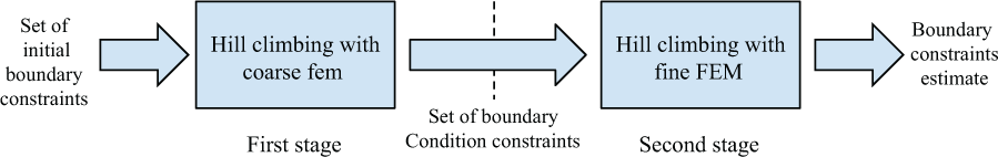
Block diagram shows the two-stage hill climbing algorithm. A set of random initial boundary constraints
3.3. Multi-stage hill climbing algorithm
The two-stage hill climbing algorithm can be expanded into a multi-stage hill climbing algorithm by employing FEM mesh refinement, as shown in Figure 2. The two critical aspects of the multi-stage hill climbing algorithm are the choice of the initial boundary constraint seeds at each iteration stage, and the choice of the termination condition. These two aspects will be discussed in the following two subsections.
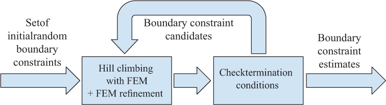
Multi-stage refining hill climbing algorithm.
3.4. Choosing boundary constraint seeds
Local extrema are an important concern for the proposed hill climbing algorithm, as the optimization being performed is not convex. Using a set of initial seeds is a common method employed in non-convex optimization to avoid local extrema. However, it is important to note that the computational cost significantly increases as the FEM mesh is refined. Therefore, it is desirable to limit the number of initial seed points used in the later iterations of the multi-stage refining algorithm.
In the earlier stages of the algorithm, the primary concern is coverage, i.e. exploring as much of the solution space as possible. On the other hand, in the subsequent stages, the concern shifts toward refining and confirming estimates obtained in the earlier iterations.
Generally speaking, we have found that using the candidates from the previous stage (possibly by adding perturbations to increase diversity) as initial seeds for the next iteration works well in most cases.
There are two choices of an initial set for the candidates that can be used at an iteration. The first choice is to use all of the local maxima obtained at the end of the previous iteration step as candidates for the next refining step. Using this scheme, it is possible to keep the diversity of peaks from different hills. A better candidate is defined by the candidate that has a greater δ value. The best local maximum (i.e. the local maximum with the highest similarity measure δ) can be reported as the best candidate of the boundary constraints.
An alternative choice is to keep track of all boundary constraint states,
3.5. Termination condition
Several different termination conditions can be used to terminate the iteration of the multi-stage hill climbing algorithm (Figure 2.) The exemplary termination conditions are below.
3.5.1. No improvement in boundary identification
In this case, the iteration is terminated if the optimal boundary constraint identified remains unchanged at consecutive iterations, i.e.
3.5.2. No improvement in the δ function
In this method, the iteration is terminated when the δ function value for the optimal boundary constraint value identified at the end of the iteration is above a given threshold. 4
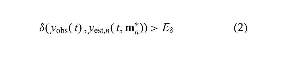
where Eδ is the termination threshold, and
3.5.3. No improvement in the FEM refinement
In this method, the iteration is terminated, if refining the FEM mesh does not improve the value of the δ function. Specifically, the scheme checks the difference between the current FEM reconstruction and the finer FEM reconstruction. The termination condition is the following
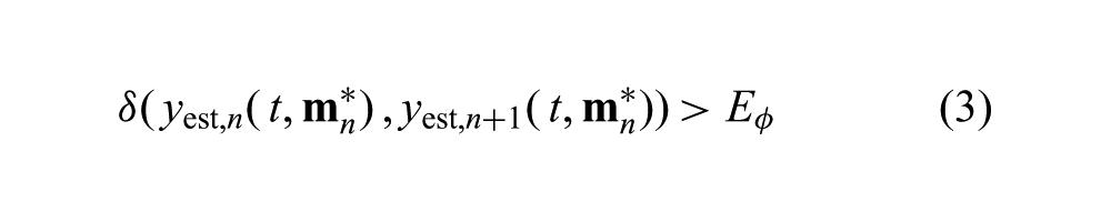
where Eϕ is the termination threshold for FEM refinement, yn is the current FEM reconstruction and yn+1 is the refined FEM reconstruction. The advantage of using this termination condition is that it is more robust to uncertainties. There are two drawbacks to using this termination condition. First, there is an extra computation required to check this termination condition. Second, one needs to be aware that this termination condition may terminate the algorithm too soon if Eϕ is set too low.
4. Active boundary exploration
The choice of the manipulation motion is critical for accurately determining boundary constraint of the object being manipulated (as it will be demonstrated later in Sections 5.2 and 6.2). In this section, we will propose an information maximization based active exploration algorithm for boundary constraint identification.
The goal of the active boundary constraint exploration algorithm is to optimally select the grasp points and manipulation actions in order to maximize the information about the boundary constraints for the object. In the proposed method, we will use a probabilistic formulation and pose action selection as an entropy minimization problem (e.g. Choset et al., 2005; Thrun et al., 2005; LaValle, 2006).
4.1. Modified boundary constraint identification
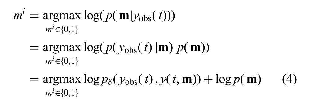
We will start by slightly modifying the boundary constraint identification method we have presented in Section 3, by using a probabilistic interpretation. Specifically, we will start by assuming that the error between the estimated and actual fiducial trajectories for a given boundary constraint and manipulation action, is random noise. Then the similarity measure defined in (1) would become a random variable. Further assuming that a model of this similarity measure’s statistics is available, in the form of the associated probability density function pδ(·), the hill climbing algorithm for boundary constraint identification (Algorithm 1) can be interpreted as maximum a posteriori (MAP) estimation by rewriting line 4 as
Using this formulation, it is also possible to construct an iterative Bayes filter for estimating beliefs for the boundary constraints of the object
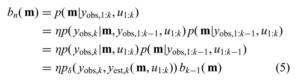
where bi(
It is important to note that the evaluation of the probability pδ in (5) is a very costly computation as it requires an FEM simulation of the object deformations. Therefore, in the implementation of the algorithm, the belief is only evaluated for the boundary constraint configurations visited during the hill climbing, in order to limit the computational complexity.
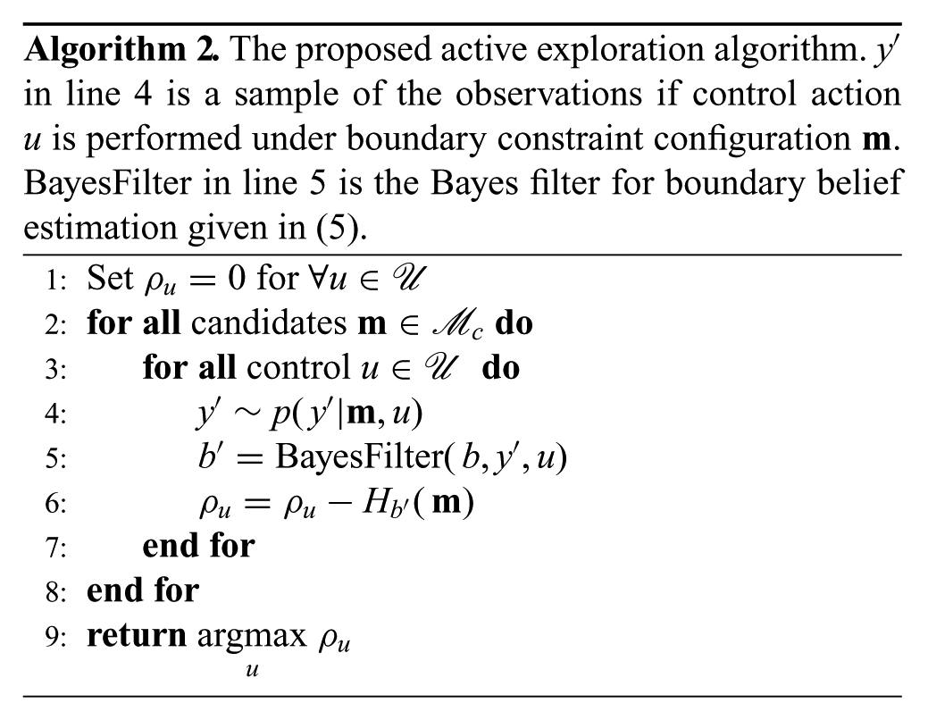
4.2. Active exploration algorithm
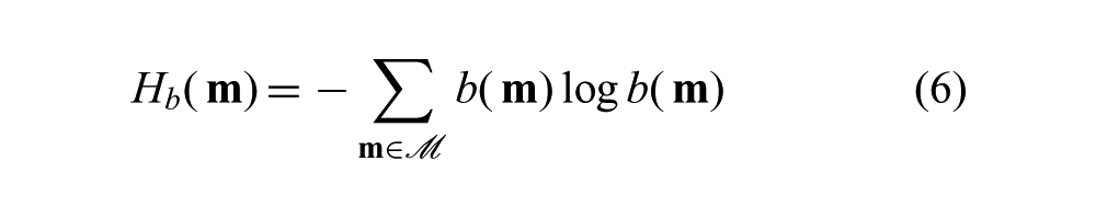
In this study, we employed a greedy active exploration algorithm based on entropy minimization. The entropy of the belief b(
Given the possible grasp point choices
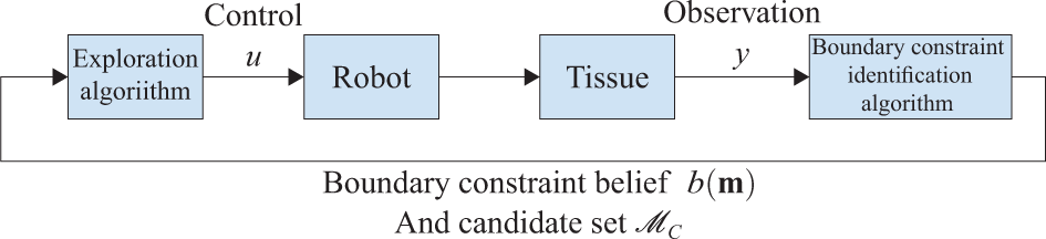
The iterative active exploration process.
As discussed above, the belief update (line 5 in Algorithm 2) is computationally very expensive, as it requires the FEM simulation of the deformable object for the control action and boundary configurations being considered. In order to limit the computational cost, the entropy estimations are calculated only for a small subset (
5. Simulation studies for validation of the identification algorithm
In this section, we will present a set of simulation studies conducted to validate the proposed boundary constraint identification algorithm.
Nonlinear finite element models were used to model the deformation of the soft tissues. The nonlinear finite element model presented here makes use of a nonlinear strain tensor and has a nonlinear stress–strain relationship (i.e. both geometric and material nonlinearities are included). The model of the tissue we used is the neo-Hookean material model (Wu, 2002; Nienhuys, 2003). The neo-Hookean material model captures the nonlinear nature of material, while its parameters still have good physical interpretation. However, it is important to note that the use of the neo-Hookean material type is not a requirement of the proposed method. Different material types can be substituted without any notable change to the method. One might consider using a simpler model for more real-time capability such as in De Pascale et al. (2004). For simplification, the analyses were performed for the quasi-static case, neglecting the inertial and damping effects in the tissue dynamics. This is not a restrictive assumption, since manipulation velocities and bandwidths are small in typical surgical manipulations.
In most of the simulation studies, a square tissue model, shown in Figure 4, with dimensions 100 × 100 × 10 mm was used. The shape was selected in order to simplify the manufacturing process of the phantom for hardware experiments (Section 6) and to make the analysis of the algorithm simpler and more intuitive. (In the last set of simulation experiment repeated in Section 5.4, a more irregular shape object is used to evaluate the method.) The end-effector gripper was assumed to grasp a 20 × 20 mm area on the object edge without a slip. This grasp was modeled by anchoring the grabbed part of the tissue rigidly to the gripper by position boundary constraints. The stress and strain of the phantom are assumed to be zero at the rest state of the object including the effect of gravity. 16 artificial fiducials were marked uniformly on the top surface of the object. These fiducials were assumed to be tracked by a calibrated stereo camera to measure their trajectories in 3D during manipulations. None of the fiducials were located on the constrained patches. The baseline observation data were generated using high density mesh model (with 3122 nodes and 13,473 elements.)
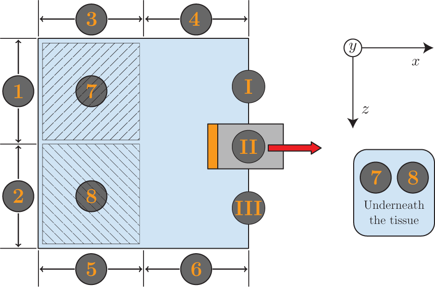
The figure shows the top view of the deformable object model used for simulation studies. The dimensions of the square object specimen used in the simulation and experimental studies is 100 × 100 × 10 mm. The patches used to cluster groups of boundary nodes are also labeled by numbers identifying where they are on the surface of the phantom. Patches 1–6 are located on the edges of the square in the figure. Patches 7 and 8 are located at the bottom side of the phantom, each covering the corresponding quarter of the bottom surface. These patches are typically not visually observable as they are covered by the object. I, II, and III are the grasp points, which will be discussed in the exploration simulation and experiment sections (Sections 7 and 8). The gripper is holding the grasp point II in the experiments in Sections 5 and 6.
The
Without loss of generality, we simplified the model to have eight pre-selected patches, as shown in Figure 4. The tissue phantom can be anchored at any patch labeled from 1 to 8 in Figure 4. All the simulations use termination condition 3 (Section 3.5.3) unless otherwise noted.
In this section, two different end effector trajectories, namely “semicircle movement” (Figure 5a) and “complex movement” (Figure 5b), were used to explore the effects of input trajectories on the identification accuracy.
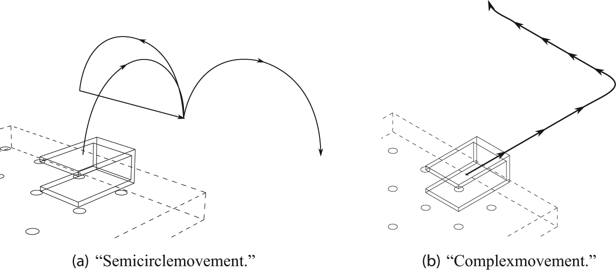
The two different end-effector trajectories used to evaluate the algorithm.
In the “semicircle movement,” the end effector first moves in a semicircle motion toward the pull direction (x-axis), followed by a second semicircle motion toward the −z-axis and a third semicircle motion toward the +z-axis. The radius of each of the semicircular segments is 10 mm. Unless otherwise stated, all the experiments in Section 5 were conducted using the “semicircle movement.”
In the “complex movement” the end effector moves diagonally ~ 28 mm in [1, 1, 1]T direction; followed by ~29 mm in [0, 0, −1]T direction; and a twist motion in the end of the trajectory.
5.1. Evaluation of two-stage hill climbing strategy
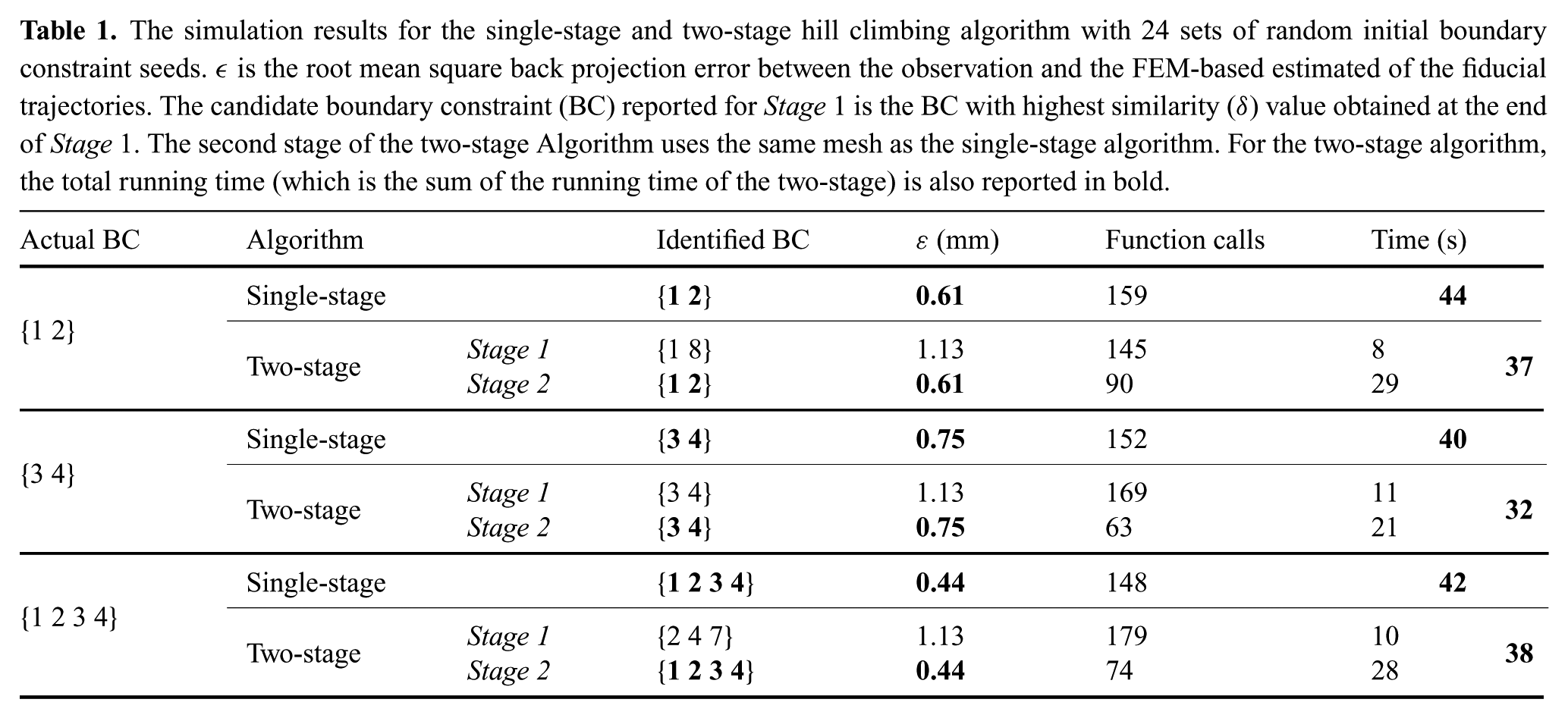
The first set of simulation results focuses on demonstrating the advantage of the two-stage hill climbing strategy over the single-stage algorithm. Three sets of simulations with three different actual boundary constraints, namely, {1 2}, {3 4}, and {1 2 3 4}, were conducted. The coarse and fine meshes used in the two-stage algorithm had 23 and 148 nodes and 37 and 379 elements, respectively, while the single-stage algorithm used only the fine mesh. The results comparing the single-stage and the two-stage algorithms are summarized in Table 1. In each of the three cases, the two-stage algorithm was able to identify the boundary constraints accurately, and with shorter computation time, by taking advantage of the low computational load of the coarse FEM mesh. The coarse FEM mesh used in the first stage was very approximate and could not necessarily accurately identify the boundary constraints. However, the candidate boundary set obtained at the end of the first stage was refined using the fine FEM mesh (with small number of function calls) to accurately identify the boundary constraints at the end of the second stage.
The simulation results for the single-stage and two-stage hill climbing algorithm with 24 sets of random initial boundary constraint seeds. ε is the root mean square back projection error between the observation and the FEM-based estimated of the fiducial trajectories. The candidate boundary constraint (BC) reported for Stage 1 is the BC with highest similarity (δ) value obtained at the end of Stage 1. The second stage of the two-stage Algorithm uses the same mesh as the single-stage algorithm. For the two-stage algorithm, the total running time (which is the sum of the running time of the two-stage) is also reported in bold.
5.2. Sensitivity of the algorithm
In this section, the results of the simulation studies performed to evaluate the robustness of the algorithm to uncertainties in the tissue’s constitutive parameters, measurement of the fiducial trajectories, and perceived end-effector motions are presented.
5.2.1. Robustness to uncertainties in tissue constitutive parameters
In this experiment, the algorithm assumed material constitutive parameters of 15 kPa for Young’s modulus and 0.35 for Poisson’s ratio, while the material parameters used for generating the baseline observation data was varied.
In the first test, the Young’s modulus, E, of the actual material was varied from 5 kPa to 30 kPa. The algorithm was able to accurately identify the boundary constraints with a success rate of 100%. In the second test, the Poisson’s ratio, ρ, of the actual material was varied from 0 to 0.49. The algorithm was again able to accurately identify the boundary constraints with a success rate of 100%. Finally, both E & ρ were simultaneously varied. The algorithm was still able to accurately identify the boundary with a success rate of 100%.
The results are summarized in Table 2. Note that the metric,
The results show the success rates of the algorithm and average back propagation errors
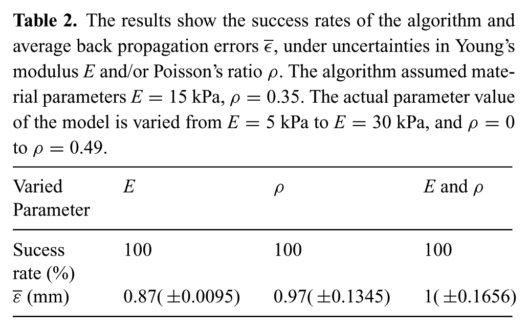
It is also interesting to note that Young’s modulus plays a less important role compared to the Poisson’s ratio. Young’s modulus relates to force perception while the Poisson’s ratio measures how the object is contracting when it is being stretched. Thus, Poisson’s ratio effects the visually perceived deformation of the object more than Young’s modulus does. The results in Table 2 reflect this observation. Uncertainty in a parameter, like Poisson’s ratio, tends to result in larger errors. As the changes in the back projection errors are small, we can neglect the influence of the parameter knowledge uncertainties.
5.2.2. Robustness to uncertainties in measurement of fiducial trajectories and robot control
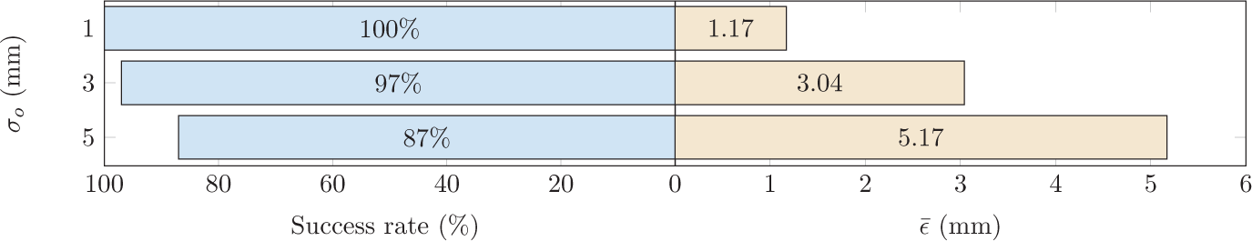
The first set of simulation studies was conducted to evaluate whether the algorithm could accurately identify the boundary constraints under uncertainties in retrieving the fiducial positions. This is evaluated by adding Gaussian white noise with varying standard deviations (σo) to the fiducial measurements. The results are shown in Figure 6.
Percentage of accurate boundary constraint detections by the algorithm under the “semicircle movement” with uncertainties in grasping location. σc is the standard deviation of the Gaussian noise added on x-axis and z-axis simultaneously.
The second set of simulation studies was conducted to evaluate the effectiveness of the algorithm when there were uncertainties in the movements of the end-effector holding the target tissue. This is evaluated by introducing Gaussian white noise with varying standard deviations (σr) to the robot trajectories in each step. The results are shown in Figure 7.
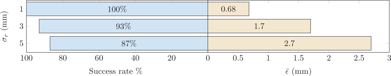
Percentage of accurate boundary constraint detections by the algorithm under the “semicircle movement” with uncertainties in robot control. σr is the standard deviation of the Gaussian noise added per axis.
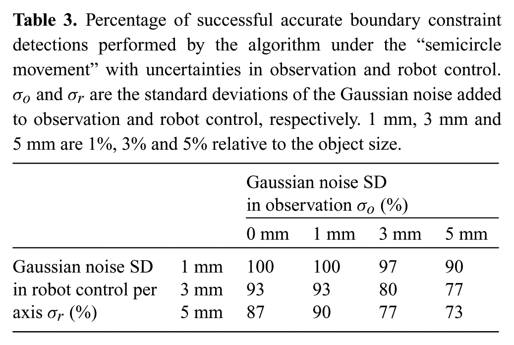
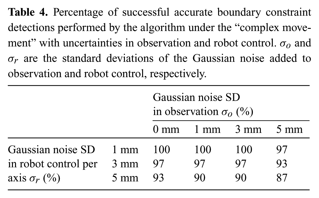
The third set of simulation studies was conducted with uncertainties in both the observed fiducial trajectories and the robot control by varying the Gaussian white noise as shown in Table 3. This experiment was also repeated with the robot performing “complex movement.” Results for this experiment are reported in Table 4.
Percentage of successful accurate boundary constraint detections performed by the algorithm under the “semicircle movement” with uncertainties in observation and robot control. σo and σr are the standard deviations of the Gaussian noise added to observation and robot control, respectively. 1 mm, 3 mm and 5 mm are 1%, 3% and 5% relative to the object size.
Percentage of successful accurate boundary constraint detections performed by the algorithm under the “complex movement” with uncertainties in observation and robot control. σo and σr are the standard deviations of the Gaussian noise added to observation and robot control, respectively.
The results reported in Figures 6 and 7 were collected from 100 random experiments and the results reported in Tables 3 and 4 were collected from 30 random experiments. All the experiments were performed using the multistage algorithm presented in Section 3.3.
The results from all of the cases above demonstrated the robustness of the algorithm. It is also informative to consider cases when the algorithm failed. For most of the cases when the algorithm failed to identify the correct boundary constraint, the boundary constraints estimated by the algorithm were rather close to the accurate answer. For instance, for the case in Table 3, some of the inaccurate answers, when the algorithm failed to get the actual answer {1 2}, were {1 5}, {1 8}, {1 2 5} and {2 7}. Similarly, for the case in Table 4, the inaccurate answers were {1 2 5}, {1 5} and {2, 3}. These results show that the performance of the algorithm degraded gracefully from the accurate answer as the uncertainties grew.
5.2.3. Robustness to uncertainties in grasping location
This set of simulation studies was conducted to evaluate the effect of end effector grasping mislocation. This is evaluated by adding Gaussian white noise with varying standard deviations (σc) to the grasping location in the x-axis and z-axis. The noise was added in the simulations used to generate the observed fiducial trajectories while the noise free grasp locations were used in the estimation. We assumed that every grasp was successful (there was no mislocation on y-axis). The results reported in Figure 8 were collected from 100 random experiments.
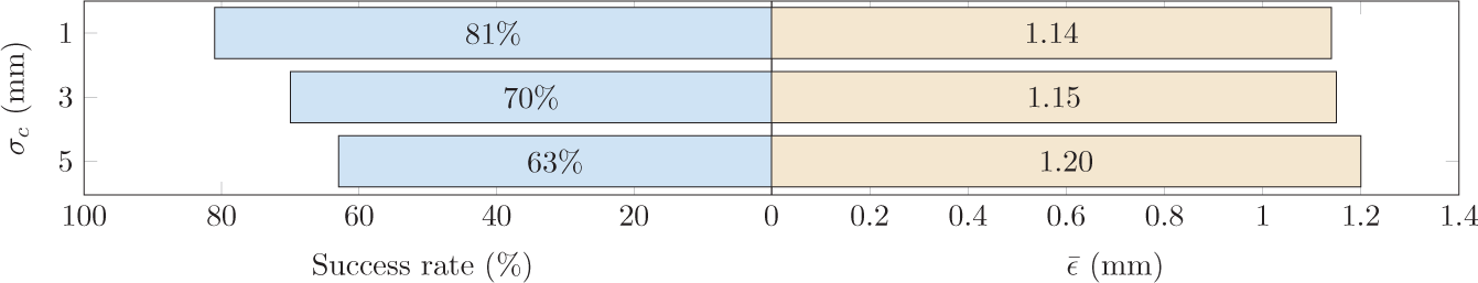
Percentage of accurate boundary constraint detections by the algorithm under the “Semicircle Movement” with uncertainties in grasping location. σc is the standard deviation of the Gaussian noise added per axis.
The results indicate that the algorithm was able to identify boundary constraints reasonably well for small errors. However, performance degraded for longer errors. This is due to the fact that grasp location errors lead to systematic (non-random) errors between the observed and estimated fiducial trajectories.
5.3. Computation time of the multi-stage algorithm
The meshes used for iteration steps n = 1 and n = 2 are the same as the coarse mesh and fine mesh used in the two-stage Hill Climbing algorithm. The meshes used for iteration steps n = 3 and n = 4 have 674 and 3122 nodes and 2134 and 13,473 elements, respectively.
The computation time range for the experiments reported in Table 3 represented as total time is 55.89−2658 s, and the average computation time is 84.28 s. The average computation time spent for iteration steps n = 1, 2, 3 are respectively 14.63 s, 33.97 s and 35.68 s. The average number of function calls for iteration steps n = 1, 2, 3 are respectively 165, 94 and 0.9.
The computation time range for the experiments reported in Table 4 represented as total time is 51.48−2632 s, and the average computation time is 67.87 s The average computation time spent for iteration steps n = 1, 2, 3, 4 are respectively 18.40 s, 38.87 s, 9.06 s and 1.53 s. The average number of function calls are 167, 100, 1.3 and 0.004 for iteration steps n = 1, 2, 3, 4.
It is important to note that the computation time significantly increases if the multi-stage algorithm needs to go to higher iterations (n = 3 or n = 4) requiring computations with finer FEM mesh densities. However, most of the time, the algorithm terminates at the lower iteration values (n = 2), as can be seen from the lower function call counts for n = 3, 4. This is why worst case computation times are significantly higher than the average computation time of the algorithm.
5.4. Example: Boundary constraint identification with irregular geometry object
The boundary constraint identification examples presented earlier in the paper were primarily conducted using solid square shapes in order to allow simpler explanations of the results. In this example, the boundary constraint identification algorithm is validated using an object model with a more irregular shape.
The manipulation scenario considered is based on surgical manipulations performed in laparoscopic cholecystectomy procedures. Cholecystectomy is the surgical procedure for removal of the gallbladder (e.g. Pitcher et al. (1995)). In this procedure, the gallbladder is dissected from the liver bed and removed after the cystic duct is clipped and cut (Figure 9(a)). The objective of the simulated surgical manipulation task is to determine whether the connective tissue around the gallbladder model has been properly dissected or not, and if not, identifying the part which is still connected.
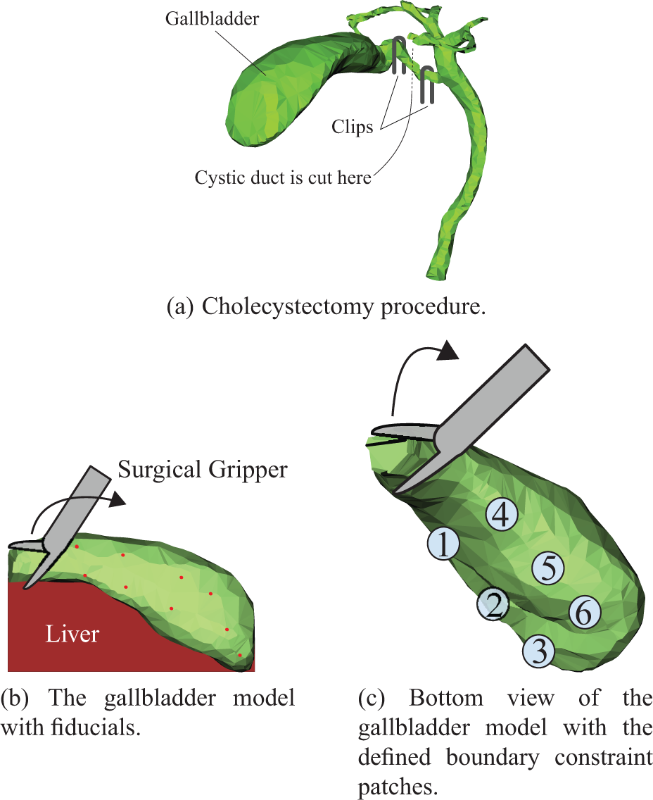
Model used from validation of boundary constraint identification with an irregular geometry object.
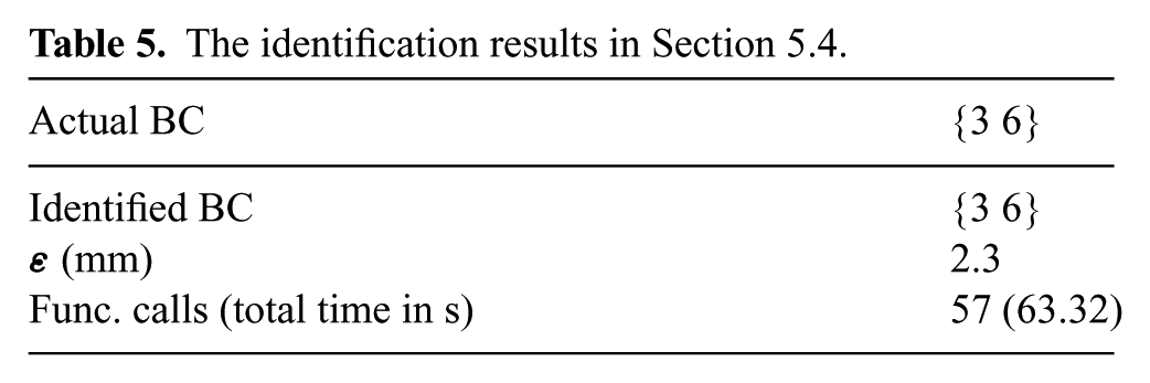
The gallbladder phantom was modeled at the end of the cystic duct as a solid object. 5 The tissue being dissected was simulated using a high density model meshed with 505 nodes and 1507 tetrahedral elements. The boundary constraint identification was performed using a 195 node and 505 tetrahedral element mesh model. Nine fiducials were marked on the tissue model (Figure 9(b)). Six patches were pre-selected, as shown in Figure 9(c). In Figures 9(b)–(c) a robotic grasper was holding the gallbladder neck and manipulating on the left side while the right side was connected to connective tissue. The result of the identification is shown in Table 5, which demonstrates that the proposed algorithm was able to successfully identify the accurate boundary constraint.
The identification results in Section 5.4.
6. Physical experiments for validation of the identification algorithm
6.1. Experiment setup
In order to validate the proposed method, physical experiments were conducted. A soft tissue phantom created using Ecoflex® 00-30, a two-part silicone rubber with Silicone Thinner® (non-reactive silicone fluid), from Smooth-On Inc. was used in the experiments. This material has been used to build tissue phantoms in a number of earlier studies (e.g. Hollenstein 2008; Boonvisut et al. 2012a; 2012b). The silicone phantoms with three different consistencies, obtained by changing the silicone thinner ratio, were used in order to cover a wide range of parameter values. ABB IRB 140, a 6 DOF robot was used to collect the manipulation trajectories. The repeatability of the robot is 0.03 mm. The setup of the experiments is shown in Figure 10.
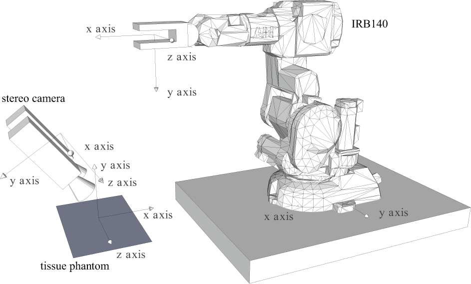
The setup of the experiments with the ABB IRB 140. The square tissue phantom created using Ecoflex® 00-30 and the dimensions of the specimen are 100 × 100 × 10 mm.
The tissue phantoms used in the experiments were same in shape and size to the models used in the simulation studies described in Section 5. Specifically, the tissue phantoms were square in shape, with dimensions of 100 × 100 × 10 mm.
Next, 16 artificial fiducials were attached to the top surface of the tissue and were tracked by a calibrated stereo camera pair to measure their deformations during retraction. Specifically, the silicone surface was labeled with rubber beads 1 mm in diameter which were used as the fiducials (Figure 11). The stereo vision system, which employed two identical FL2G-13S2C 1.3MP cameras (Point Gray Research, Richmond, BC, Canada), were used to measure the surface deformations during manipulation. The cameras were placed at a distance of 30 cm. The cameras were programmed using the Flycapture library (Point Gray Research, Richmond, BC, Canada) and OpenCV. Once the fiducials were detected, and their correspondences in the stereo image pair determined, the actual locations of the fiducials were estimated by triangulation using the camera calibration information.
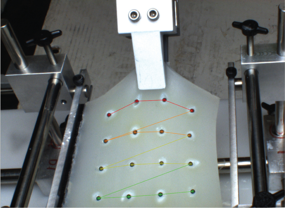
The robot performing “Gradual Tangent Pull” to retract the Ecoflex 00–30 tissue with mixture ratio 1:1:2 anchored at {1 2 3 4}.
The tissue phantoms were placed horizontally while being grabbed and retracted by a gripper towards the right. Figure 11 shows the view as seen from the robot cameras. The tissue phantom was anchored on the bottom and left of the figure, which are the patches {1 2} and {3 4} defined in Figure 4, respectively. The anchored patches could be selected from the black plastic strips attached to the tissue phantom. (Only the left strip can be seen in Figure 11.) Round rare earth magnets were put inside both the black plastic strips and the tissue stage to ensure a strong adhesion.
The retraction actions were achieved by moving the gripper in 1–2 mm increments, towards the right, producing about 10% elongation of the tissue phantom as shown in Figure 12. The “pull” trajectory was performed in 10 steps with 2 mm increments; the “gradual tangent pull” (“GTP”) trajectory was performed in 20 steps with ~ 2 mm increments; and the “twist and pull” (“T&P”) trajectory was performed in 10 steps with ~ 2 mm increments.
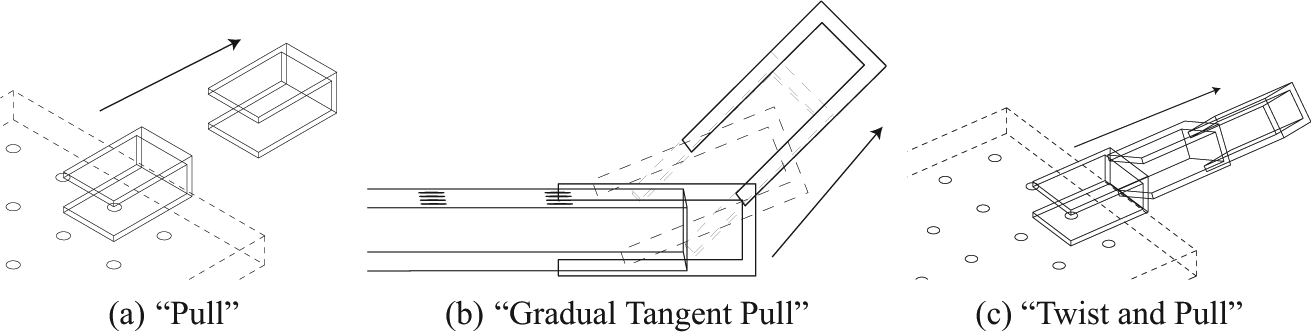
Figures show the different types of end-effector motions used to evaluate the boundary constraints.
6.2. Physical experiment results
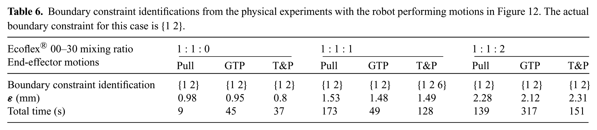
The experiments were conducted for two separate boundary constraint cases. Table 6 shows the results when the phantom tissue has one side anchored, namely, patches {1 2} as defined in Figure 4. On the other hand, Table 7 shows the results when the phantom has two sides anchored, namely, {1 2 3 4}. Three different silicone mixing ratios were used 1 : 1 : 0, 1 : 1 : 1 and 1 : 1 : 2. (A : B : T is proportion of part A of the silicone, part B of the silicone and silicone thinner by mass. The specimen gets softer as the proportion of the silicone thinner is increased.)
Boundary constraint identifications from the physical experiments with the robot performing motions in Figure 12. The actual boundary constraint for this case is {1 2}.
Boundary constraint identifications from the physical experiments with the robot performing motions in Figure 12. The actual boundary constraint for this case is {1 2 3 4}.
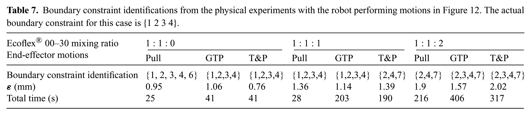
All of the results reported in Tables 6 and 7 can be characterized as reasonable, even though the boundary constraints were not accurately identified as {1 2} and {1 2 3 4} in some of the cases. Inaccurate boundary identifications are {1 2 6} in the first case and {1 2 3 4 6}, {2 4 7} and {2 3 4 7} in the second case, which were qualitatively close to the actual boundary constraints, and gave comparable back projection errors (
7. Simulation studies for validation of the active exploration algorithm
The simulation setup is similar to the setup used in the simulation studies in Section 5. In order to increase the richness of the possible control action space, two additional possible grasp point choices were added at two sides side of the original grasp point in Figure 4. Then three grasping location are 30 mm apart. Also, the possible manipulation actions were limited to six directions (±x, ±y, ±z). Here, we used the single-stage identification algorithm in Section 3.1. The multi-stage identification algorithm in Section 3.3 can be replaceable.
7.1. Validation under accurate tissue motion measurements
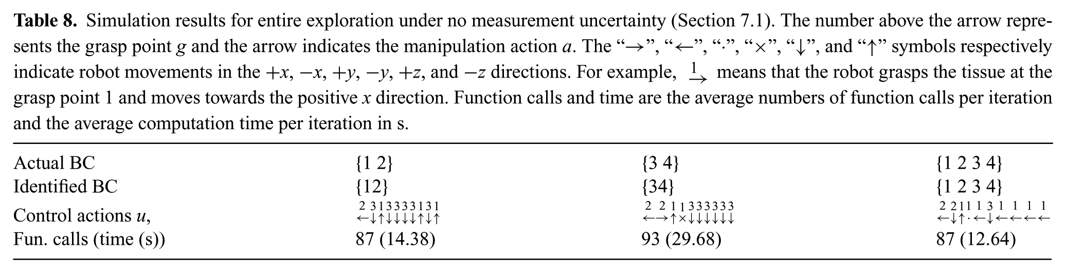
The first set of simulation studies were conducted to validate if the proposed algorithm can accurately identify the tissue boundary constraints under ideal conditions, i.e. no error in fiducial motion measurements is produced. The results of the simulation studies for the exploration of three different boundary constraint cases are presented in Table 8 and Figure 13. The results indicate that the proposed active exploration algorithm was successful in identifying the boundary constraints.
Simulation results for entire exploration under no measurement uncertainty (Section 7.1). The number above the arrow represents the grasp point g and the arrow indicates the manipulation action a. The “→”, “←”, “·”, “×”, “↓”, and “↑” symbols respectively indicate robot movements in the +x, −x, +y, −y, +z, and −z directions. For example,
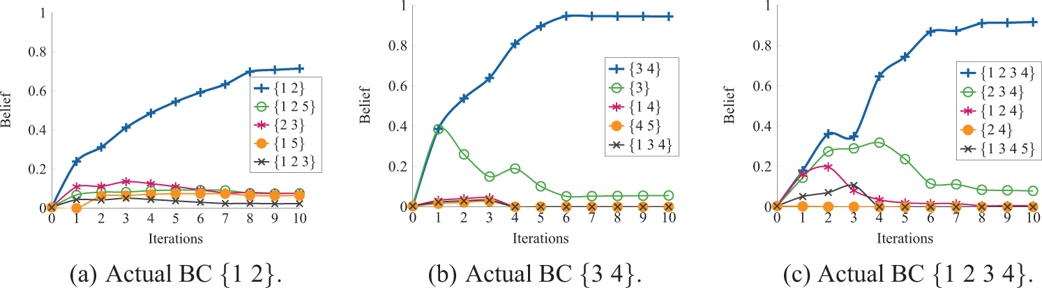
The progression of the belief values of the candidate boundary constraint configurations as a function of the iteration step of the active exploration algorithm (Section 7.1). The corresponding experiment results are presented in Table 8.
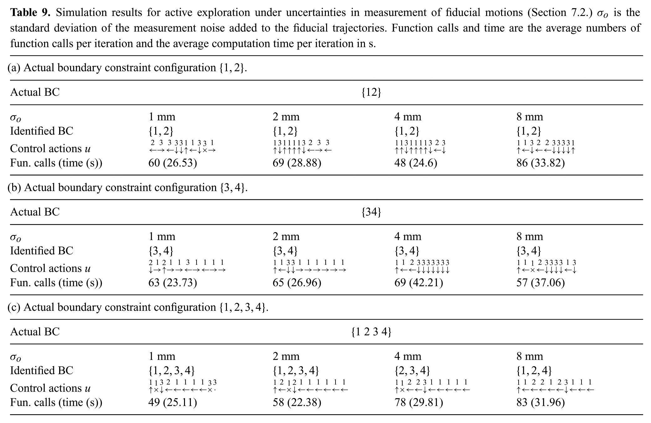
7.2. Sensitivity of the exploration algorithm to uncertainties
The second set of simulation studies was conducted to evaluate the robustness of the active exploration approach to noise in tissue deformation measurements (i.e. fiducial motion measurements). Here, for conciseness, we have only reported analysis of the exploration algorithm to uncertainties in only fiducial motion measurements, as errors in visual measurements of fiducial motions would typically dominate the errors in robot motions. For example, in our experimental setup, the repeatability of the robot system is about 0.03 mm, while the back projection error of our stereo camera system is about 0.3 mm. The measurement uncertainties are similar to those used in Section 5.2.2. 6
The results shown in Table 9 demonstrate that the proposed approach can effectively identify boundary constraints at low noise levels, and performance degrades gracefully for large noise levels.
Simulation results for active exploration under uncertainties in measurement of fiducial motions (Section 7.2.) σo is the standard deviation of the measurement noise added to the fiducial trajectories. Function calls and time are the average numbers of function calls per iteration and the average computation time per iteration in s.
8. Physical experiments for evaluation of the active exploration algorithm
We have conducted experiments on a physical experimental platform to evaluate the effectiveness of the active exploration algorithm. The experimental setup used was similar to the setup used in Section 6.1. In these experiments, tissue phantoms with only 1 : 1 : 0 mixing ratio of the EcoFlex silicone were used.
We have limited the strains that the manipulated object is subjected to by limiting the gripper displacements to 8 mm for each action (about 1/2 of the total displacement used in the experiments in Section 6), and requiring the object to be returned to the zero strain configuration at the end of each manipulation action. Limiting the tissue strains made the boundary constraint identification problem more challenging as this results in fiducial trajectories with smaller displacements.
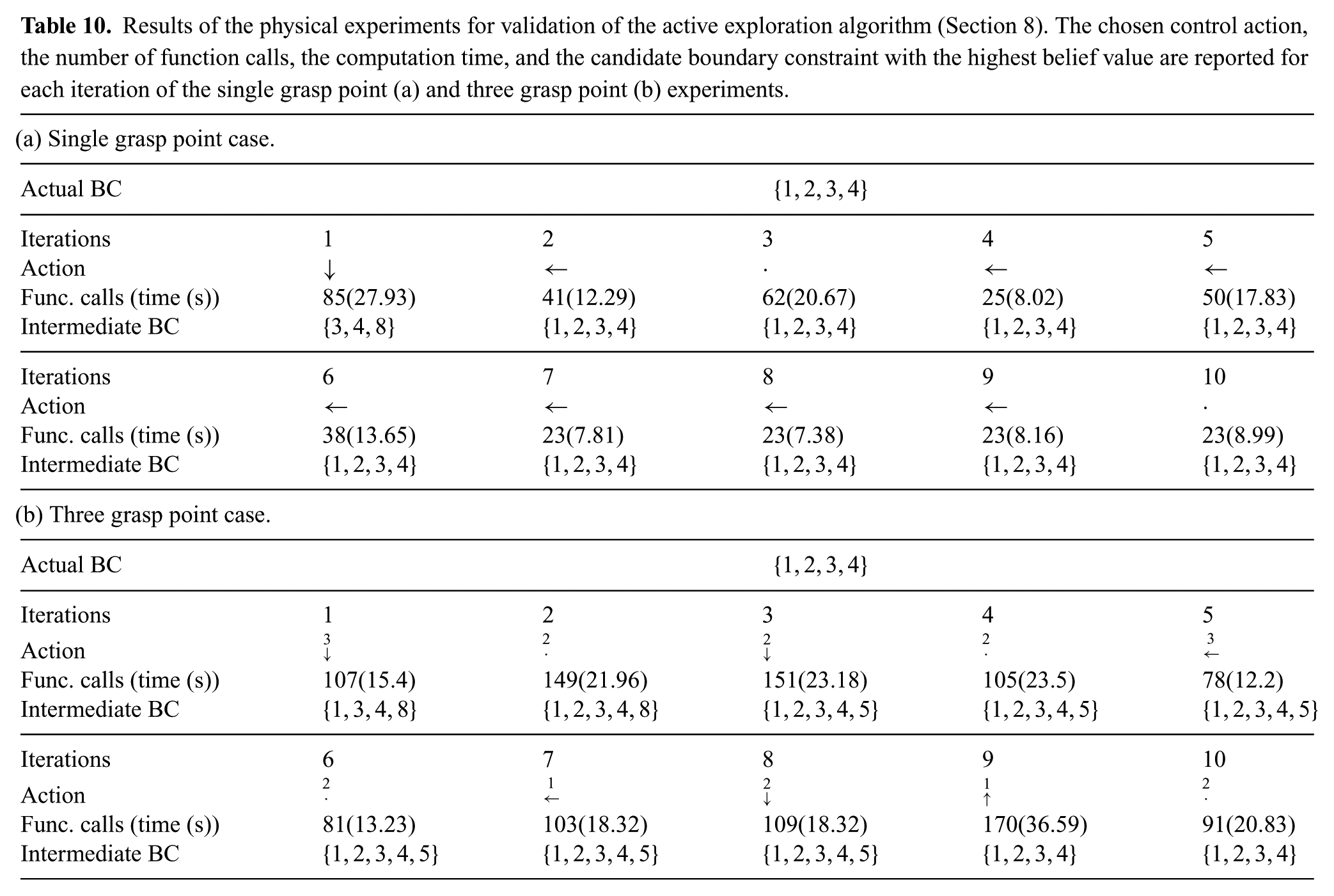
We have conducted two sets of experiments. In the first set of experiments, the robotic tool was allowed to use only a single grasp point. In the second set of experiments, the algorithm was allowed to grasp the tissue at three different grasp points, similar to the configuration used in the simulation studies (Section 7). The results of the first case are shown in Table 10(a) and Figure 14(a), and the results of the second case are shown in Table 10(b) and Figure 14(b). The experiment results demonstrated that the algorithm was able to successfully identify the boundary constraints.
Results of the physical experiments for validation of the active exploration algorithm (Section 8). The chosen control action, the number of function calls, the computation time, and the candidate boundary constraint with the highest belief value are reported for each iteration of the single grasp point (a) and three grasp point (b) experiments.
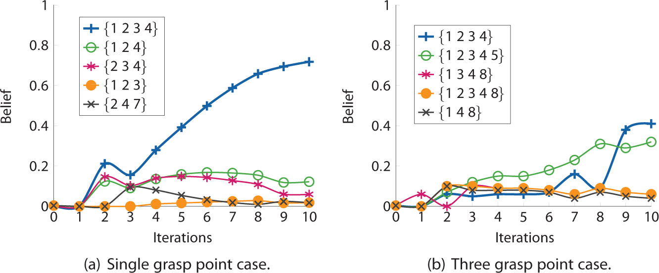
Results of the physical experiments for validation of the active exploration algorithm (Section 8). Progression of the candidate boundary constraint configurations’ belief values are shown for the single grasp point (a) and three grasp point (b) cases.
9. Discussion and conclusions
In this paper, an algorithm for the identification of boundary constraints of deformable objects during robotic manipulation was presented. The core of the algorithm was inspired by the hill climbing algorithm used to solve occupancy grid estimation problems in mobile robotics. The information regarding the boundary constraints of the deformable object obtained using the proposed methods can potentially be used for both off-line planning or on-line (real-time) re-planning of object’s manipulation.
The experimental and simulation results demonstrated the robustness of the proposed algorithm to uncertainties. Most notably, the algorithm was capable of coping with uncertainties in the object’s constitutive parameters. Therefore, in applications where both the object material properties and the boundary constraints are unknown, the boundary constraint identification can be performed before the estimation of the constitutive parameters of the object.
However, it should be noted that, a priori information regarding the constitutive parameters of the object may benefit the accuracy of the algorithm, especially by improving the back projection errors.
The influence of the choice of the robot trajectory on identification of the boundary constraints has been illustrated by the results reported in Tables 3 and 4. In order to address this issue, an active exploration algorithm based on an information maximization formulation was proposed. This algorithm was also validated by simulation and hardware experiments.
The presented algorithms need to be further optimized for online operation. The algorithms are very suitable for parallelization. The individual iterations of the main computation loop of the boundary identification algorithm (lines 2–5 in Algorithm 1) are mutually independent and can be trivially parallelized. (In the presented simulation results, the algorithms were executed in eight parallel threads.) Similarly, the individual iterations of the inner loop of the active exploration algorithm (lines 3–7 in Algorithm 2) are mutually independent and can be trivially parallelized. Another avenue for improving the computation time would be to use a faster FEM engine.
In the formulation of the modified boundary constraint identification and active exploration algorithms, the error in the estimation of the fiducial trajectories was modeled as random noise (see Section 4.1). Systematic errors in the algorithm used for estimation of fiducial trajectories, namely yest(t,
The present study only focused on identification of boundary constraints (identification of the subset of a deformable object’s boundary that is assumed to be rigidly anchored in space. Modeling the influence of more complex boundary interactions (such as, attachment to other deformable objects, sliding contact with unpredictable amounts of friction, etc.) is outside the scope of this study. Extension of the proposed algorithms to model and identify such complex boundary conditions is an important avenue of further research.
This work has considered only passive deformations of objects. Active deformable objects, in which the objects have active internal forces are outside the scope of the present study. Manipulation of active deformable objects, such as manipulation of a beating heart in robotic cardiac surgery (Nakamura et al., 2001; Bebek and Çavuşoğlu, 2007; Richa and Poignet, 2009; Yuen et al., 2009; Tuna et al., 2013), brings interesting challenges. As the active internal forces result in non-random perturbations, they would need to be explicitly modeled to avoid systematic errors in the probabilistic algorithm.
Manipulations that result in topological changes in the deformable object (such as, cutting, tearing, etc.) are also outside the scope of the current study.
The different FEM meshes (including the refinements) used in the experiments were manually pre-generated. The mesh refinement was uniform throughout the object, including boundary constraint and fiducial areas. In a practical application, the meshes of the objects that are being manipulated can potentially be generated from a priori data (such as, pre-operative medical diagnostic images in a surgical application). An automatic adaptive online refinement algorithm can also potentially be used as part of the proposed algorithm. An online algorithm which employs on-line mesh refinement can potentially be more flexible but at the expense of substantial computation.
Similarly, boundary constraint patches used in the simulation and hardware experiments were pre-generated. Automatic sectioning of patches and automatic patch refinement, which was not pursued in this work, might be interesting to explore.
In this study, FEM was used to model the object deformations. Alternative modeling approaches (such as mass-spring-damper models) which may have computational advantages can potentially be considered. However, care should be taken with regards to systematic errors with such models (Natsupakpong and Çavuşoğlu, 2010).
Footnotes
Funding
This work was supported in part by NSF (grant numbers IIS-0905344 and CNS-1035602) and National Institutes of Health (grant numbers R21 HL096941 and R01 EB018108).