Evasion paths in mobile sensor networks

Abstract

Suppose that ball-shaped sensors wander in a bounded domain. A sensor does not know its location but does know when it overlaps a nearby sensor. We say that an evasion path exists in this sensor network if a moving intruder can avoid detection. In ‘Coordinate-free coverage in sensor networks with controlled boundaries via homology', Vin de Silva and Robert Ghrist give a necessary condition, depending only on the time-varying connectivity data of the sensors, for an evasion path to exist. Using zigzag persistent homology, we provide an equivalent condition that moreover can be computed in a streaming fashion. However, no method with time-varying connectivity data as input can give necessary and sufficient conditions for the existence of an evasion path. Indeed, we show that the existence of an evasion path depends not only on the fibrewise homotopy type of the region covered by sensors but also on its embedding in spacetime. For planar sensors that also measure weak rotation and distance information, we provide necessary and sufficient conditions for the existence of an evasion path.

Keywords

Mobile sensor networks coverage pursuit-evasion homology zigzag persistence fibrewise embeddings

1. Introduction

In minimal sensor network problems, one is given only local data measured by many weak sensors but tries to answer a global question (Estrin et al., 2002; Gao and Guibas, 2012). Tools from topology can be useful for this passage from local to global. For example, Baryshnikov and Ghrist (2009) combine redundant local counts of targets to obtain an accurate global count using integration with respect to Euler characteristic. Coverage problems are another class of problems in minimal sensing: when sensors are scattered throughout a domain, can we determine whether the entire domain is covered? See Ahmed et al. (2005), Fan and Jin (2010), Ghosh and Das (2008), and Wang (2011) for surveys of coverage problems, and see de Silva and Ghrist (2006, 2007) for topological approaches.

We are interested in the following mobile sensor network coverage problem from de Silva and Ghrist (2006). Suppose that ball-shaped sensors wander in a bounded domain. A sensor cannot measure its location but does know when it overlaps a nearby sensor. We say that an evasion path exists if a moving intruder can avoid being detected by the sensors. Can we determine whether an evasion path exists? We refer to this question as the evasion problem. The evasion problem can also be described as a pursuit–evasion problem in which the domain is continuous and bounded, there are multiple sensors searching for intruders, and an intruder moves continuously and with arbitrary speed. We do not control the motions of the sensors; the sensors wander continuously but otherwise arbitrarily. We cannot measure the locations of the sensors but instead know only their time-varying connectivity data. Using this information, we would like to determine whether it is possible for an intruder to avoid the sensors. See Chung et al. (2011) for a survey of related pursuit–evasion problems, and see Liu et al. (2005) and Chin et al. (2010) for scenarios in which the motion of the sensors or intruders can be controlled.

After introducing the evasion problem, de Silva and Ghrist (2006) give a necessary homological condition for an evasion path to exist. Using zigzag persistent homology, we provide an equivalent condition that moreover can be computed in a streaming fashion. However, it turns out that homology alone is not sufficient for the evasion problem. Indeed, neither the fibrewise homotopy type of the sensor network nor any invariants thereof determine whether an evasion path exists; we show that the fibrewise embedding of the sensor network into spacetime also matters. Knowing this, we provide necessary and sufficient conditions for the existence of an evasion path for planar sensors that can also measure weak rotation and distance data.

In Section 2 we provide background material on fibrewise spaces. We define the evasion problem in Section 3, and in Section 4 we describe the work of de Silva and Ghrist. We introduce zigzag persistence in Section 5 and apply it to the evasion problem in Section 6. However, zigzag persistence does not give a complete solution to the evasion problem. Indeed, in Section 7 we show the existence of an evasion path depends not only on the fibrewise homotopy type of the sensor network but also on the ambient isotopy class of its embedding in spacetime. In Section 8 we restrict attention to planar sensors measuring cyclic orderings and provide an if-and-only-if result. We conclude in Section 9 and describe possible directions for future work.

2. Fibrewise spaces

Since we are studying mobile sensors, both the region covered by the sensors and the uncovered region change with time. In this section we encode the notion of time-varying spaces using the language of fibrewise spaces. We also consider fibrewise maps between fibrewise spaces, what it means for two fibrewise maps to be fibrewise homotopic, and what it means for two fibrewise spaces to be fibrewise homotopy equivalent. See Crabb and James (1998) for more information on fibrewise homotopy theory.

A fibrewise space is a space equipped with a notion of time. More precisely, let I = [0, 1] be the closed unit interval. A fibrewise space is a topological space Y equipped with a continuous map p: Y→I to time; see Figure 1 for an example. For any point y ∈ Y one can think of p(y) as the time coordinate associated to this point. Given two fibrewise spaces p: Y→I and p′: W→I, a continuous map f: Y→W is said to be fibrewise if p′○f = p. In other words, a fibrewise map is time-preserving. A section for a fibrewise space p: Y→I is a fibrewise map s: I→Y, that is, a continuous map s: I→Y with p(s(t)) = t for all t ∈ I.

Fig. 1.

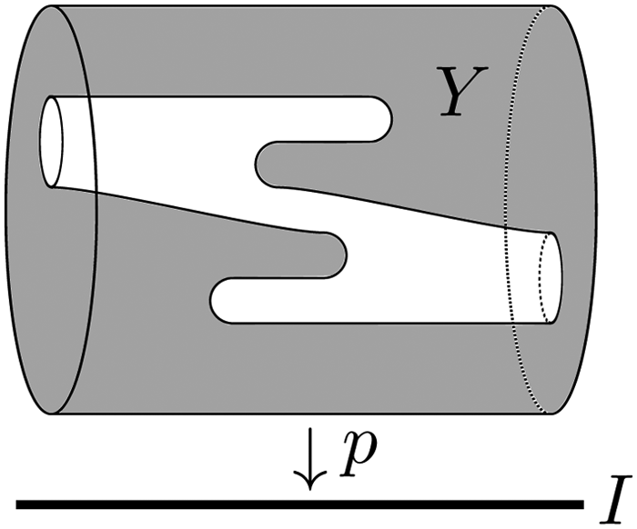
A fibrewise space p: Y→I.

Roughly speaking, two fibrewise maps are fibrewise homotopic when one can be deformed to the other in a time-preserving manner. More precisely, two fibrewise maps f₀, f₁: Y→W are fibrewise homotopic if there is a homotopy F: Y × I→W with F( , 0) = f₀, with F( , 1) = f₁, and with each F( , t) a fibrewise map. The homotopy F gives a continuous and time-preserving deformation from f₀ to f₁. Two fibrewise spaces are fibrewise homotopy equivalent when they are homotopy equivalent in a time-preserving manner. More explicitly, a fibrewise map f: Y→W is a fibrewise homotopy equivalence if there is a fibrewise map f′: W→Y with compositions f′○f and f○f′ each fibrewise homotopic to the corresponding identity map; in this case we say that fibrewise spaces Y and W are fibrewise homotopy equivalent.

3. The evasion problem

The evasion problem we consider is introduced by de Silva and Ghrist (2006), and we present it here with a few minor changes. Let $D \subset R^{d}$ be a bounded domain homeomorphic to a d-dimensional ball, where d ≥ 2. Suppose that a finite set S of sensor nodes moves inside this domain over the time interval I = [0, 1], with each sensor v ∈ S a continuous path $v : I \to D$ . We assume that two distinct sensors never occupy the same location: for sensors $v \neq \tilde{v}$ we have $v (t) \neq \tilde{v} (t)$ for all t. Let $B_{v (t)} = {y \in D ‖ v (t) - y ‖ \leq 1}$ be the unit ball covered by sensor v at time t. The sensors cannot measure their locations but two sensors do know when they overlap. This allows us to measure the time-varying connectivity graph of the sensors. The connectivity graph at time t has the set of sensors S as its vertex set and has an edge between sensors v and $\tilde{v}$ when $B_{v (t)} \cap B_{\tilde{v} (t)} \neq \emptyset$ ; see Figure 2(b). We assume there is an immobile subset of fence sensors whose union of balls contains the boundary $\partial D$ and is homotopy equivalent to $\partial D$ .

Fig. 2.

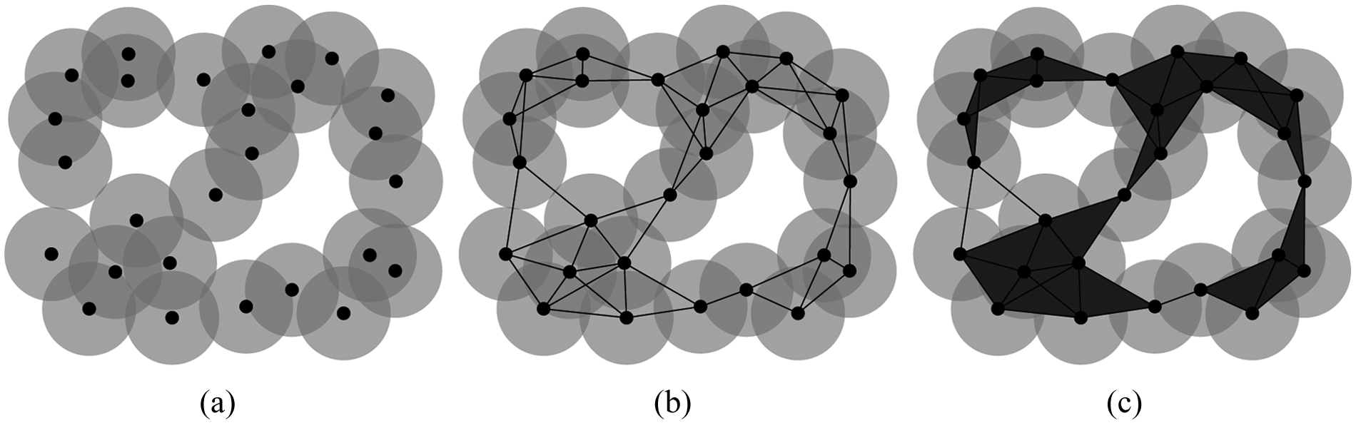
(a) A sensor network at a fixed point in time, (b) its connectivity graph, and (c) its $\overset{⌣}{C}$ ech complex.

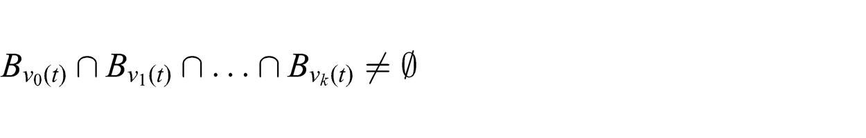
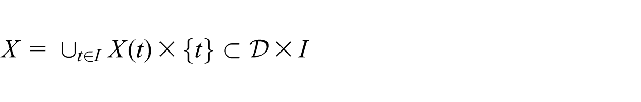
The union of the balls X(t) = ∪_v ∈ S B_v(t) is the region covered by the sensors at time t, and its complement $X {(t)}^{c} = D ∖ X (t)$ is the uncovered region at time t. Let

X = \cup_{t \in I} X (t) \times {t} \subset D \times I

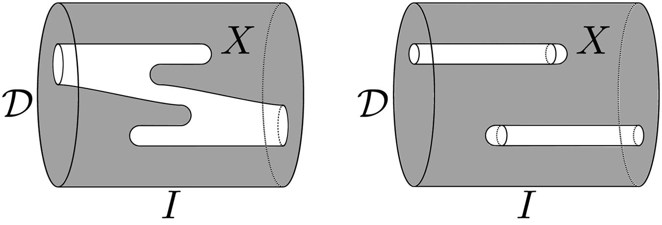
be the subset of spacetime covered by sensors, and let $X^{c} = (D \times I) ∖ X$ be the uncovered region in spacetime. Both X and X^c are fibrewise spaces, that is, spaces equipped with projection maps X→I and X^c →I to time. See Figure 3 for two examples.

Fig. 3.

We have drawn two planar sensor networks with domain $D \subset R^{2}$ on the vertical axis and with time I on the horizontal axis. The region X in spacetime covered by the sensors is drawn in gray, and the uncovered region X^c is drawn in white. The network on the left contains an evasion path. The network on the right does not contain an evasion path because an intruder must move continuously and cannot teleport locations.

Potentially there are also intruders moving continuously in this domain. The intruders would like to avoid being detected by the sensors, but an intruder is detected at time t if it lies in the covered region X(t). We say that an evasion path exists when it is possible for a moving intruder to avoid being seen by the sensors.

Definition 1. An evasion path in a sensor network is a section s: I→X^c of the projection map p: X^c →I. Equivalently, an evasion path is a continuous map $s : I \to D$ such that s(t)∉X(t) for all t.

Given a sensor network, we would like to determine whether or not an evasion path exists. However, connectivity graphs alone cannot determine the existence of an evasion path. Consider the two sensor networks in Figure 4, and suppose that in each case all three sensors are immobile over the entire time interval. Then the two networks have the same connectivity graphs at each point in time, but the sensor network on the left contains an evasion path while the network on the right does not.

Fig. 4.

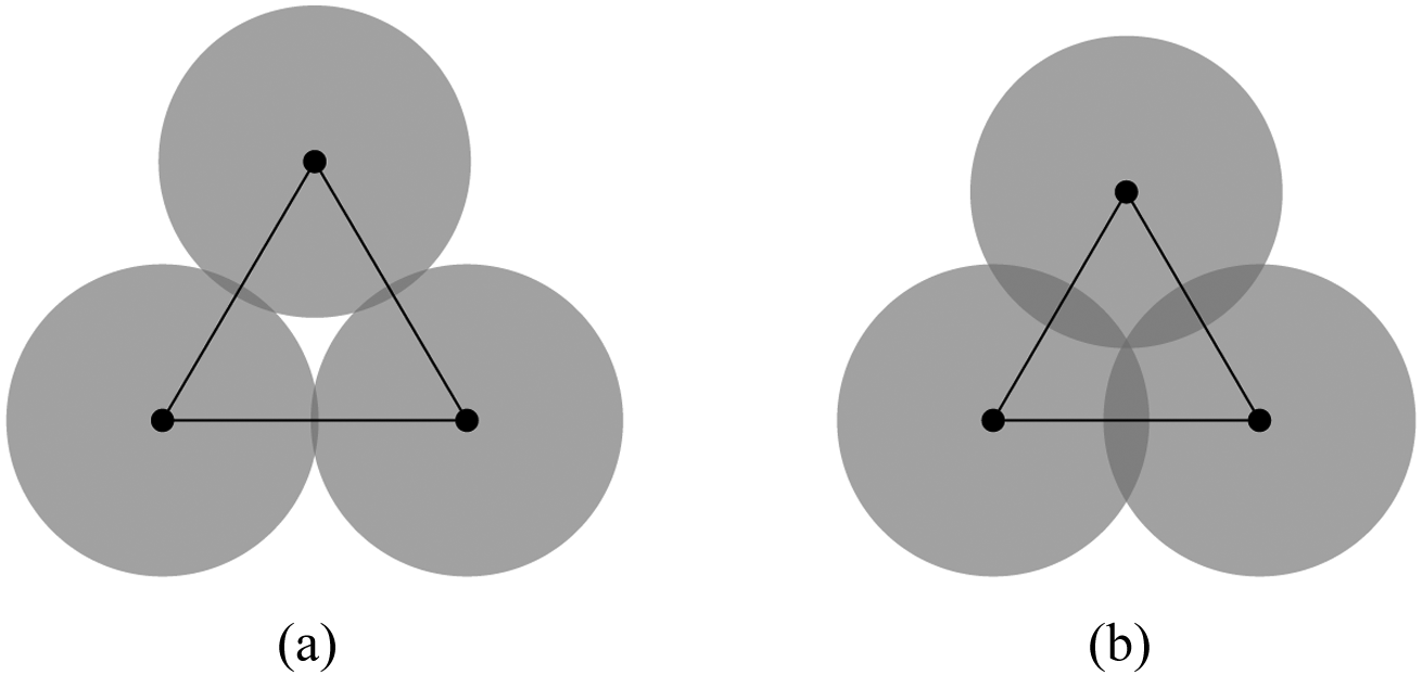
Let (a) and (b) be two different sensor networks. Imagine that no sensor moves over the entire time interval. Then network (a) has an evasion path while network (b) does not, even though the two networks have the same connectivity graph at each point in time.

Since connectivity graphs alone are insufficient, we consider $\overset{⌣}{C}$ ech simplicial complexes encoding higher connectivity information. The $\overset{⌣}{C}$ ech simplicial complex C(t) of the sensors is the nerve of the unit balls {B_v(t) }_v∈S (Edelsbrunner and Harer, 2010). This means that the vertex set of C(t) is the set of sensors S, and we have a k-simplex when the intersection of the corresponding (k+1)-balls is non-empty. That is, simplex [v₀ v₁…v_k ] is in C(t) when

B_{v_{0} (t)} \cap B_{v_{1} (t)} \cap \dots \cap B_{v_{k} (t)} \neq \emptyset

See Figure 2(c) for an example. Note that the 1-skeleton of C(t) is the connectivity graph at time t. An important property is that the $\overset{⌣}{C}$ ech complex C(t) is homotopy equivalent to the union of the balls X(t) by the nerve lemma (Hatcher, 2002, Corollary 4G.3). We are now ready to state the evasion problem.

The Evasion Problem. Given the time-varying $\overset{⌣}{C}$ ech complex C(t) of a sensor network over all times t ∈ I, can one determine whether an evasion path exists?

Remark 1. One can recover the fibrewise homotopy type of the covered region X of a sensor network from the time-varying $\overset{⌣}{C}$ ech complex.

Remark 2. In the static setting in which the sensors do not move, one can use the $\overset{⌣}{C}$ ech complex to determine whether or not the sensors cover the entire domain $D$ . The evasion problem asks whether an analogous statement is true in the setting of mobile sensors.

In applications it is generally unreasonable to assume that our sensors can measure $\overset{⌣}{C}$ ech complexes. This would require the task of detecting k-fold intersections, which is not possible under many models of minimal sensing. However, we can approximate the $\overset{⌣}{C}$ ech complex from either above or below using the Vietoris–Rips complex (Vietoris, 1927). The Vietoris–Rips complex is the maximal simplicial complex built on top of the connectivity graph, and hence can be recovered by sensors measuring only two-fold overlaps. This approximation allows us to take results based on $\overset{⌣}{C}$ ech complexes and produce analogous approximate results using only Vietoris–Rips complexes; see the Appendix for more details. For example, the results of de Silva and Ghrist (2006) are stated in terms of Vietoris–Rips complexes. We avoid such approximations and instead use $\overset{⌣}{C}$ ech complexes.

We make the simplifying assumption that each sensor covers a unit ball. With the exception of Section 8 on alpha complexes and the Appendix, all of our results also hold in the more general setting where each sensor covers an arbitrary convex set. In this setting the $\overset{⌣}{C}$ ech complex becomes the nerve of the convex sets.

4. The work of de Silva and Ghrist

In order to explain de Silva and Ghrist’s work on the evasion problem, we first define the stacked $\overset{⌣}{C}$ ech complex. The stacked $\overset{⌣}{C}$ ech complex is a single cell complex encoding the $\overset{⌣}{C}$ ech simplicial complexes C(t) for all times t∈I. We assume there are only a finite number of times

0 < t_{1} < \dots < t_{n} < 1

when the $\overset{⌣}{C}$ ech complex changes. Hence, for t and t′ in either (t_i , t_i+1), [0, t₁), or (t_n , 1], we have C(t) = C(t′). Moreover, we assume that at each time t_i simplices are either added to or removed from the $\overset{⌣}{C}$ ech complex but not both. Since the sensor balls are closed, a simplex σ is:

added at time t_i when σ ∈ C(t_i ) but σ∉C(t) for t ∈ (t_i − 1,t_i ); and

removed at time t_i when σ ∈ C(t_i ) but σ∉C(t) for t ∈ (t_i , t_i+1)

Choose interleaving times

0 = s_{0} < t_{1} < s_{1} < \dots < t_{n} < s_{n} = 1

Definition 2. The stacked $\overset{⌣}{C}$ ech complex p: SC→I is the fibrewise space obtained from the disjoint union $∐_{i = 0}^{n} C (s_{i}) \times [t_{i}, t_{i + 1}]$ , where t₀ = 0 and t_{n + 1} = 1, by identifying:

C(s_i − 1) × {t_i } as a subset of C(s_i ) ×{t_i }; if simplices are added at t_i and

C(s_i ) × {t_i } as a subset of C(s_i − 1) × {t_i } if simplices are removed at t_i

Map p: SC→I is the projection onto the second coordinate, and note that p ⁻¹(t) = C(t).

This definition is similar to the definition of the stacked Vietoris–Rips complex in de Silva and Ghrist (2006). See Figure 5 for a small example.

Fig. 5.

The stacked $\overset{⌣}{C}$ ech complex for three sensor nodes. The top row shows how the $\overset{⌣}{C}$ ech complex changes: initially the $\overset{⌣}{C}$ ech complex consists of an edge and a vertex, and as the sensors move closer together two more edges and a 2-simplex are added. The bottom row shows the stacked $\overset{⌣}{C}$ ech complex, obtained by adding prism cells.

A partial answer to the evasion problem is given in Theorem 7 of de Silva and Ghrist (2006). We state their result using the stacked $\overset{⌣}{C}$ ech complex instead of the stacked Vietoris–Rips complex, and for $D \subset R^{d}$ with dimension d arbitrary. Recall that a subset of immobile fence sensors covers the boundary $\partial D$ , and let F × [0,1] be the subcomplex of the stacked $\overset{⌣}{C}$ ech complex SC consisting of only these fence sensors.

Theorem 7 of de Silva and Ghrist (2006), reformulated. If there exists some [α] ∈ H_d (SC, F × [0, 1]) with 0 ≠ [∂α] ∈ H_d − 1(F × [0, 1]), then there is no evasion path in the sensor network.

We explain the picture behind this theorem. Suppose there is some

[α] \in H_{d} (SC, F \times [0, 1])

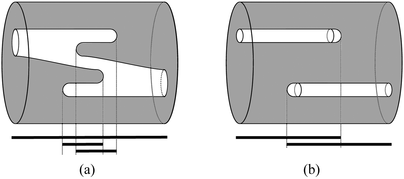
with 0 ≠ [∂α]. Let α be a relative d-cycle in SC that represents the homology class [α]. The condition 0 ≠ [∂α] means that the boundary of α wraps a non-trivial number of times around F × [0, 1]. We think of α as a “sheet” in the region of spacetime covered by the sensors that separates time zero from time one; see Figure 6(a). If there is such a relative cycle α then no evasion path can exist. For example, Theorem 7 of de Silva and Ghrist (2006) proves there is no evasion path in the sensor network in Figure 6(b).

Fig. 6.

(a) A relative 2-cycle α from Theorem 7 of de Silva and Ghrist (2006). (b) Theorem 7 of de Silva and Ghrist (2006) proves that there is no evasion path in this sensor network. (c) Although there is no evasion path in this network, Theorem 7 of de Silva and Ghrist (2006) does not apply.

Theorem 7 of de Silva and Ghrist (2006) is equivalent to the following statement: if there is an evasion path in the sensor network, then every [α] ∈ H_d (SC,F × [0,1]) satisfies 0 = [∂α]. This homological criterion is necessary but not sufficient for the existence of an evasion path. The insufficiency is demonstrated by the sensor network in Figure 6(c): every [α] ∈ H_d (SC, F × [0, 1]) satisfies 0 = [∂α], but there is no evasion path since an intruder cannot move backwards in time. Can we sharpen this theorem to get necessary and sufficient conditions?

5. Zigzag persistence

We introduce zigzag persistence in this section before applying it to the evasion problem in the following section. Zigzag persistence (Carlsson and de Silva, 2010) is a generalization of persistent homology (Edelsbrunner et al., 2002; Zomorodian and Carlsson, 2005) in which the maps can go in either direction, and zigzag persistence is also the specific case of quiver theory (Gabriel, 1972; Derksen and Weyman, 2005) when the underlying quiver is a Dynkin diagram of type A_n .

A zigzag diagram is a directed graph with n vertices and n − 1 arrows

•_{1} \leftrightarrow •_{2} \leftrightarrow •_{3} \leftrightarrow \dots \leftrightarrow •_{n - 1} \leftrightarrow •_{n}

where each arrow points either to the left or to the right. Fix a field k. A zigzag module V is a diagram

V_{1} \overset{q_{1}}{\leftrightarrow} V_{2} \overset{q_{2}}{\leftrightarrow} \dots \overset{q_{n - 2}}{\leftrightarrow} V_{n - 1} \overset{q_{n - 1}}{\leftrightarrow} V_{n}

where each V_i is a finite vector space over k and each q_i is a linear map pointing either to the left or to the right. A morphism f between two zigzag modules V and W is a diagram

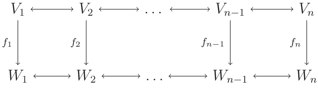
in which all of the squares commute. If each f_i is an isomorphism of vector spaces, then f is an isomorphism of zigzag modules. In the language of category theory, a zigzag module is a functor from the free category generated by a zigzag diagram to the category of finite vector spaces, and a morphism between two zigzag modules is a natural transformation (Mac Lane, 1998).

The direct sum of two zigzag modules V and V′ is given by (V⊕V′)_i = V_i⊕V_i′, with connecting linear maps of the form q_i ⊕q_i′. For birth and death indices 1 ≤ b ≤ d ≤ n, the interval module $I (b, d)$ is defined by

I {(b, d)}_{i} = {\begin{matrix} k & if b \leq i \leq d \\ 0 & otherwise \end{matrix}

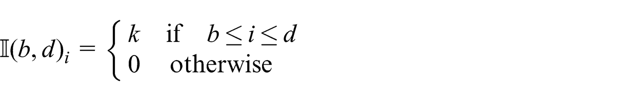
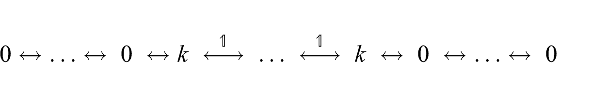
The connecting linear maps of $I (b, d)$ are identity maps $1$ between adjacent copies of the field k, and zero maps otherwise. So $I (b, d)$ looks like

0 \leftrightarrow \dots \leftrightarrow 0 \leftrightarrow k \overset{1}{\leftrightarrow} \dots \overset{1}{\leftrightarrow} k \leftrightarrow 0 \leftrightarrow \dots \leftrightarrow 0

where the first k is in slot b and the last k is in slot d. As in persistent homology, a zigzag module is described up to isomorphism by its barcode decomposition (Gabriel, 1972; Carlsson and de Silva, 2010).

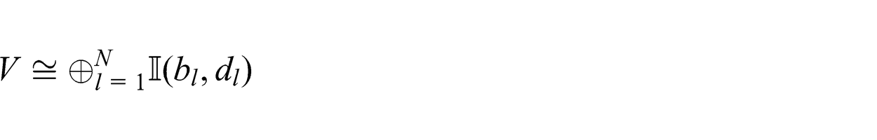
Theorem 1 (Gabriel). A zigzag module V can be decomposed as

V ≅ \oplus_{l = 1}^{N} I (b_{l}, d_{l})

where the factors in the decomposition are unique up to reordering.

A barcode is a multiset of intervals of the form [b, d], and the barcode for a zigzag module $V ≅ \oplus_{l = 1}^{N} I (b_{l}, d_{l})$ is {[b₁, d₁],[b₂, d₂,],…,[b_N , d_N ]}.

Given a fibrewise space p: Y→I and a choice of discretization

0 = s_{0} < s_{1} < \dots < s_{n} = 1

we build a zigzag module that models how the homology of fibrewise space Y changes with time. Let Y_i = p ⁻¹(s_i ) and let $Y_{i}^{i + 1} = p^{- 1} ([s_{i}, s_{i + 1}])$ . We have the zigzag diagram

Y_{0} ↪ Y_{0}^{1} ↩ Y_{1} ↪ \dots ↩ Y_{n - 1} ↪ Y_{n - 1}^{n} ↩ Y_{n}

(1)

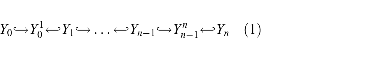
of topological spaces and inclusion maps (Carlsson et al., 2009). See Figure 7 for an example.

Fig. 7.

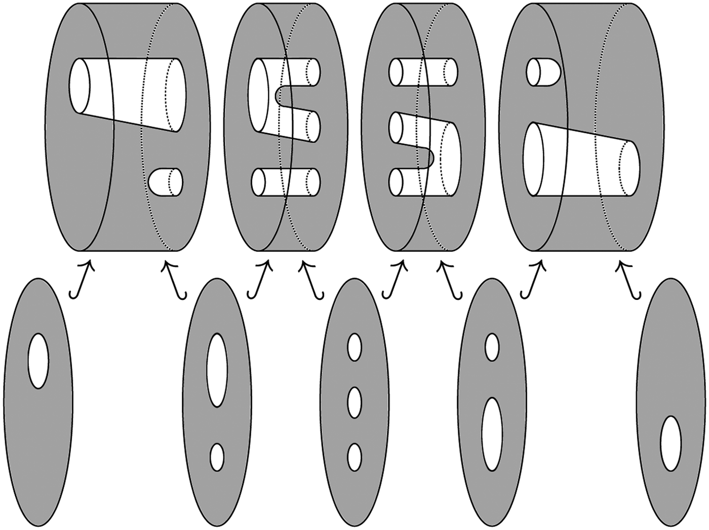
A zigzag diagram built from the fibrewise space in Figure 1.

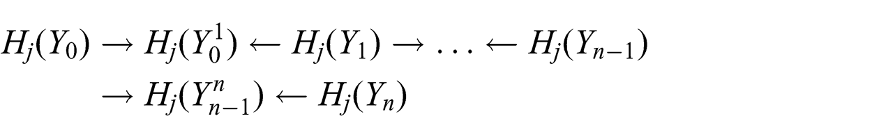
We assume that each Y_i and $Y_{i}^{i + 1}$ have finite-dimensional homology and cohomology, each taken with coefficients in a field k. Applying the j-dimensional homology functor H_j to (1) gives the zigzag module

\begin{matrix} H_{j} (Y_{0}) & \to H_{j} (Y_{0}^{1}) \leftarrow H_{j} (Y_{1}) \to \dots \leftarrow H_{j} (Y_{n - 1}) \\ \to H_{j} (Y_{n - 1}^{n}) \leftarrow H_{j} (Y_{n}) \end{matrix}

We denote this zigzag module ZH_j (Y), leaving implicit the choice of discretization and the choice of coefficient field. Applying the j-dimensional cohomology functor H^j to (1) gives the zigzag module

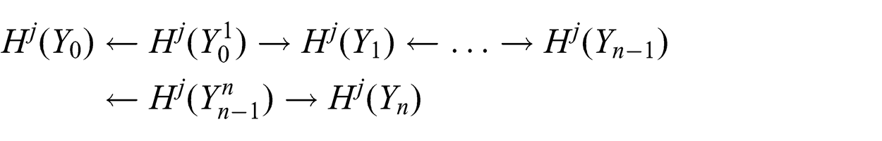
\begin{matrix} H^{j} (Y_{0}) & \leftarrow H^{j} (Y_{0}^{1}) \to H^{j} (Y_{1}) \leftarrow \dots \to H^{j} (Y_{n - 1}) \\ \leftarrow H^{j} (Y_{n - 1}^{n}) \to H^{j} (Y_{n}) \end{matrix}

which we denote ZH^j (Y). Note the directions of the arrows have been reversed because cohomology is contravariant.

The following lemmas will be useful in the proof of Theorem 2. The first lemma states that zigzag persistent homology and cohomology are invariants of fibrewise homotopy type, and the second lemma states that the barcodes for zigzag persistent homology and cohomology are identical.

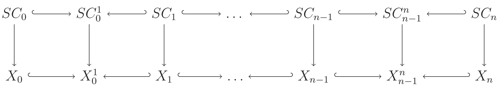
Lemma 1. If Y and W are fibrewise homotopy equivalent, then ZH_j (Y) ≅ ZH_j (W) and ZH^j (Y) ≅ ZH^j (W).

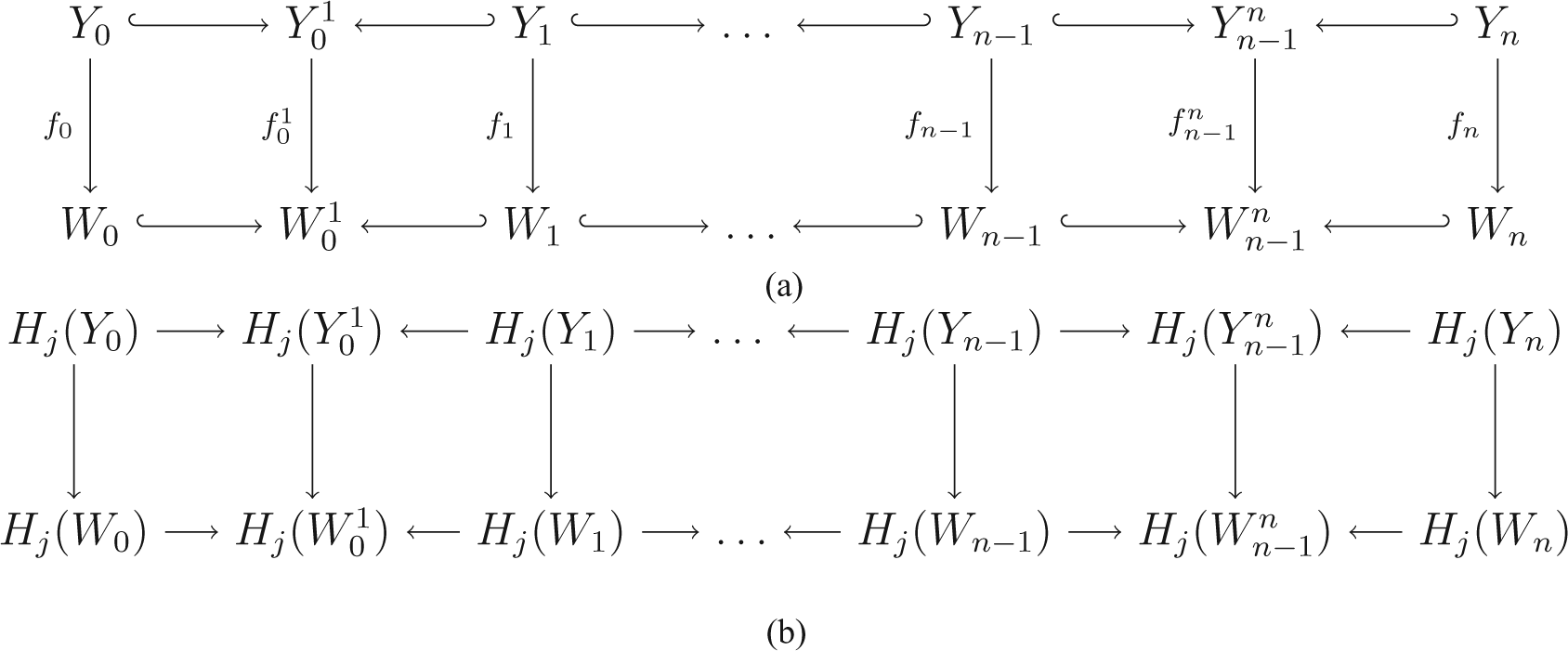
Proof. Let f: Y→W be a fibrewise homotopy equivalence. This induces the commutative diagram in Figure 8(a) where each map f_i or $f_{i}^{i + 1}$ is defined via restriction and is a homotopy equivalence. Since homology is a homotopy invariant, applying H_j gives the commutative diagram in Figure 8(b) in which each vertical map is an isomorphism. Hence, ZH_j (Y) ≅ZH_j (W). The proof for cohomology is analogous.□

Fig. 8.

Commutative diagrams for the proof of Lemma 1.

Lemma 2. The barcodes for ZH_j (Y) and ZH^j (Y) are equal as multisets of intervals.

Proof. The version of this lemma with persistent homology instead of zigzag persistence is given in Proposition 2.3 of de Silva et al. (2011), and our proof is analogous. Because their arrows point in different directions, the zigzag modules ZH_j (Y) and ZH^j (Y) live in different categories and cannot be isomorphic. However, consider the decomposition

{ZH}_{j} (Y) ≅ \oplus_{l = 1}^{N} I (b_{l}, d_{l})

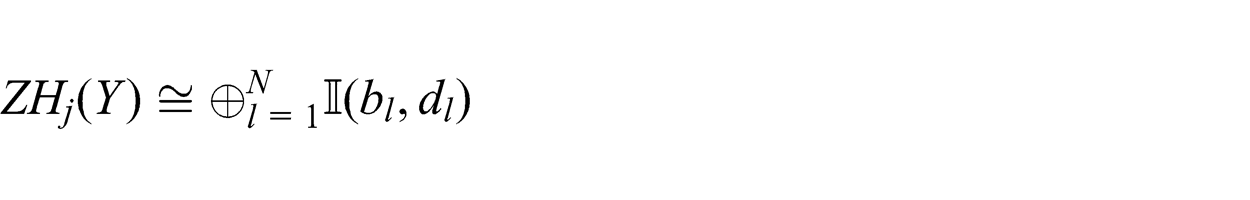
from Theorem 1. Applying the contravariant functor Hom( ;k) produces the decomposition

Hom ({ZH}_{j} (Y); k) ≅ \oplus_{l = 1}^{N} I (b_{l}, d_{l}),

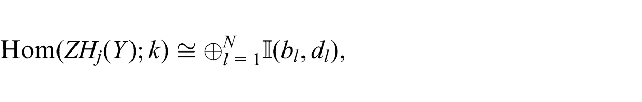
where the directions of the arrows in the zigzag modules have been reversed. Naturality of the universal coefficient theorem (Hatcher, 2002, Theorem 3.2) with coefficients in a field gives ZH^j (Y) ≅ Hom (ZH_j (Y); k), and hence the barcodes for ZH_j (Y) and ZH^j (Y) are equal as multisets of intervals.□

6. Applying zigzag persistence to the evasion problem

We began studying the evasion problem with the goal of finding an if-and-only-if criterion for the existence of an evasion path using zigzag persistence, which in this setting describes how the homology of the region covered by sensors changes with time.

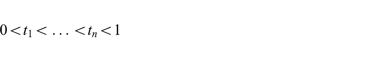
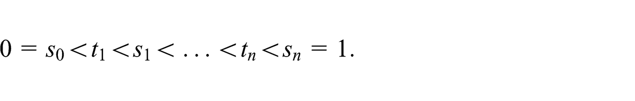
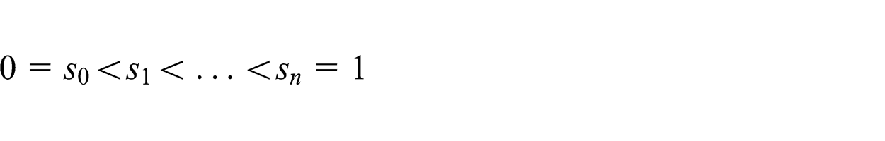
Consider the times 0 < t₁ < … < t_n < 1 when the $\overset{⌣}{C}$ ech complex changes and choose interleaving times

0 = s_{0} < t_{1} < s_{1} < \dots < t_{n} < s_{n} = 1 .

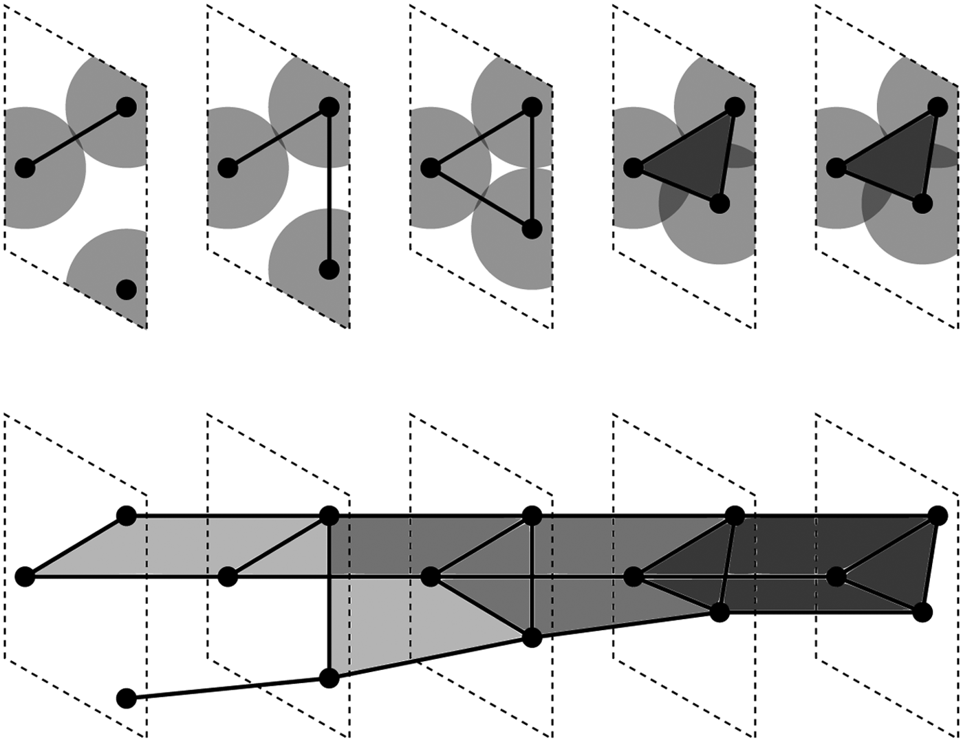
We saw in Section 5 that the discretization 0 = s₀ < s₁ < … < s_n = 1 produces a zigzag diagram of spaces from any fibrewise space, and we will consider the fibrewise spaces X, X^c , and SC. Figure 9 depicts the zigzag diagram built from a stacked $\overset{⌣}{C}$ ech complex SC.

Fig. 9.

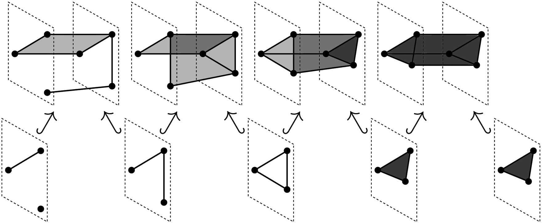
The zigzag diagram for the stacked $\overset{⌣}{C}$ ech complex from the three sensor nodes in Figure 5.

Lemma 3. For X the region of spacetime covered by sensors and SC the stacked $\overset{⌣}{C}$ ech complex, we have ZH_j (X) ≅ZH_j (SC).

Proof. By the nerve lemma we have the commutative diagram in Figure 11 with each vertical arrow a homotopy equivalence. The remainder of the proof is identical to the proof of Lemma 1.□

Our initial hypothesis was that an evasion path would exist in a sensor network if and only if there were a full-length interval [1, 2n+1] in the barcode for ZH_d − 1(SC). For example, network (a) in Figure 10 has both an evasion path and a full-length interval, and network (b) has neither. Only one direction of this hypothesis is true.

Fig. 10.

Two planar sensor networks and their barcode decompositions for ZH₁(X).

Fig. 11.

Commutative diagram for the proof of Lemma 3.

Theorem 2. If there is an evasion path in a sensor network, then there is a full-length interval [1, 2n+1] in the zigzag barcode for ZH_d − 1(SC).

Proof. An evasion path is a section s: I→X^c , that is, a commutative diagram

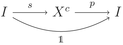
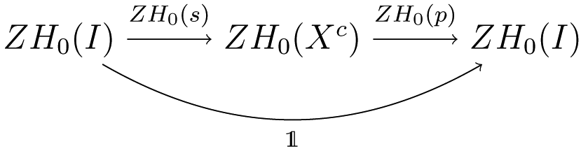
with $1$ the identity map. Applying zigzag homology ZH₀ gives the following commutative diagram.

Since the identity map on ${ZH}_{0} (I) ≅ I (1, 2 n + 1)$ factors through ZH₀(X^c ), the splitting lemma (Hatcher, 2002, Section 2.2) implies that the barcode decomposition for ZH₀(X^c ) contains a summand isomorphic to $I (1, 2 n + 1)$ . Hence, there is a full-length interval [1, 2n+1] in the barcode for ZH₀(X^c ). Next we need a version of Alexander duality (Hatcher, 2002, Theorem 3.44). We apply Theorem 3.11 of Kališnik (2013), which uses the diamond principle of Carlsson and de Silva (2010) and our Lemma 2, to obtain a full-length interval in ZH_d − 1(X). Since ZH_d − 1(X) ≅ZH_d − 1(SC) by Lemma 3, the proof is complete.□

Remark 3. This theorem is as discerning as the reformulated version of Theorem 7 of de Silva and Ghrist (2006). That is, one theorem can be used to prove that no evasion path exists in a sensor network if and only if the other theorem can be used. However, suppose that the sensors move for a long period of time. In this case the amalgamated complex used in Corollary 3 of de Silva and Ghrist (2006) to compute their homological criterion may become quite large. By contrast, the algorithm for computing zigzag persistence runs in a streaming fashion that does not require storing the sensor network across all times simultaneously. This streaming algorithm is given in Section 4 of Carlsson et al. (2009). Hence, computing our Theorem 2 may be more feasible for sensors moving over a long period of time.

Interestingly, the converse to Theorem 2 is false. This is demonstrated by the sensor network in Figure 12(a). It is tempting to guess that the barcode for this network consists of the intervals drawn on top in black, but they are crossed out because they are incorrect. The correct barcode beneath contains a full-length interval [1, 2n+1] even though there is no evasion path. We explain this counterintuitive barcode in Figure 12(b), and we give a second explanation in Section 7.

Fig. 12.

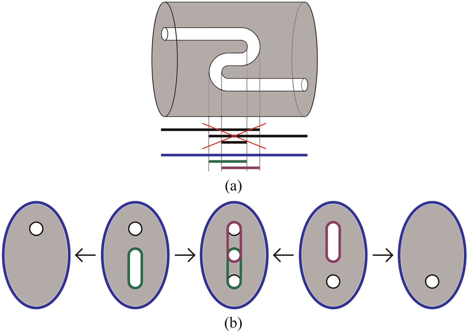
(a) It is tempting to guess that the barcode for ZH₁(X) consists of the crossed-out intervals on top in black, but instead the correct barcode is drawn beneath in blue, green, and purple. Note there is a full-length interval [1,2n + 1] even though there is no evasion path in this network. (b) A coarsened version of the zigzag diagram for X. The cycles drawn in blue, green, and purple are generators for the three intervals in ZH₁(X).

Caution 2.9 from Carlsson and de Silva (2010) explains that although every submodule isomorphic to an interval in a persistent homology module corresponds to a direct summand, the same is not true for zigzag modules. The sensor networks in Figures 10(b) and 12(a) are good examples of this caution. The zigzag modules for both sensor networks have a submodule isomorphic to the full-length interval module $I (1, 2 n + 1)$ , but Figure 12(a) contains $I (1, 2 n + 1)$ as a summand whereas Figure 10(b) does not.

7. Dependence on the embedding

It turns out that the answer to the evasion problem is no: in general, neither the time-varying $\overset{⌣}{C}$ ech complex C(t) of a sensor network nor the fibrewise homotopy type of covered region X determine if an evasion path exists. The ambient isotopy class of the fibrewise embedding of X into spacetime $D \times I$ also matters.

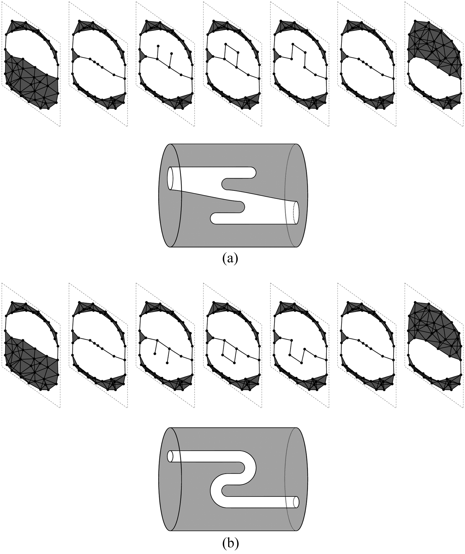
We demonstrate this impossibility result using the planar sensor networks (a) and (b) in Figure 13. Let us describe network (a). Initially, the bottom half of domain $D$ is covered by sensors. These sensors retreat to the boundary, leaving a horizontal line of sensors. Two sensors on this line jut out towards the top of $D$ , forming three sides of a square. These two sensors move closer together, completing the square. The bottom two sensors in this square move apart, breaking the bottom edge of the square. The curvy line of sensors straightens out. Finally, sensors flood from the boundary to cover the top half of $D$ . Network (b) is identical to (a) except that the square opens towards the bottom of $D$ .

Fig. 13.

Each subfigure is a sensor network represented both as seven sequential $\overset{⌣}{C}$ ech complexes and as a covered region X in spacetime D × I. At each time t ∈ I the $\overset{⌣}{C}$ ech complexes C(t) in (a) and (b) are identical. Moreover, the two covered regions are fibrewise homotopy equivalent. Nevertheless, network (a) contains an evasion path, but network (b) does not because the intruder cannot travel backwards in time.

The time-varying $\overset{⌣}{C}$ ech complexes C(t) for the two networks are identical, but network (a) has an evasion path while network (b) does not. Furthermore, the covered regions for these two networks are fibrewise homotopy equivalent, and the stacked $\overset{⌣}{C}$ ech complexes are fibrewise homeomorphic. However, the uncovered regions for the networks are not fibrewise homotopy equivalent, and in particular (a) has a section while (b) does not. Thus, the existence of an evasion path depends not only on the fibrewise homotopy type of the sensor network but also on how the sensor network is fibrewise embedded in spacetime $D \times I$ . Morover, in domain $D \subset R^{d}$ for any d ≥ 2 there exists a pair of analogous sensor networks. Analogous examples in $D \subset R^{1}$ require the sensors to turn off and then back on.

Remark 4. In the static setting in which the sensors do not move, one can use the $\overset{⌣}{C}$ ech complex to determine whether the sensors cover the entire domain $D$ . However, in the setting of mobile sensors, the time-varying $\overset{⌣}{C}$ ech complex does not in general determine if there exists an evasion path or not.

In Section 6 we promised a second explanation for the counterintuitive zigzag barcode in Figure 12(a), which we give now. The sensor network in Figure 12(a) is the same as the network in Figure 13(b), whose covered region is fibrewise homotopy equivalent to the covered region for the network in Figure 13(a). Hence by Lemma 1 their zigzag barcodes must be equal, and the zigzag barcodes for the network in Figure 13(a) are shown in Figure 10(a).

Embeddings are a central theme in topology. For topological spaces X and Y, an embedding f: X↪Y maps X injectively and homeomorphically onto its image. A typical goal is to classify the space of embeddings up to some notion of equivalence, such as isotopy or ambient isotopy, and the difficulty of this task depends heavily on the spaces X and Y. Knot theory considers the case when X is the circle and $Y = R^{3}$ , and higher-dimensional analogues are even more complicated. However, for some choices of manifolds X and Y, homotopy-based classifications for the space of embeddings do exist (Whitney, 1944; Haefliger, 1961; Adachi, 1993). For the evasion problem (and also its natural extension in which one would like to describe not only whether an evasion path exists but also the entire space of evasion paths), it would be useful to have extensions of embedding theory both to the setting of non-manifold spaces and to the setting of fibrewise spaces. One possibility is to try to adapt the tools of embedding calculus (Weiss, 1999) to a fibrewise setting.

8. Sensors measuring cyclic orderings

Since neither the time-varying $\overset{⌣}{C}$ ech complex nor the fibrewise homotopy type of covered region X are sufficient to determine whether an evasion path exists, what minimal sensing capabilities might we add? In this section we assume the sensors live in a planar domain $D \subset R^{2}$ and that each sensor measures the cyclic ordering of its neighbors, as in Ghrist et al. (2008). It is not uncommon for sensors to measure this weak angular data, for example by performing circular radar sweeps. In Theorem 3 we give necessary and sufficient conditions for the existence of an evasion path based on this rotation information.

Theorem 3 relies on the alpha complex of the sensors. Let V_v(t) be the Voronoi cell

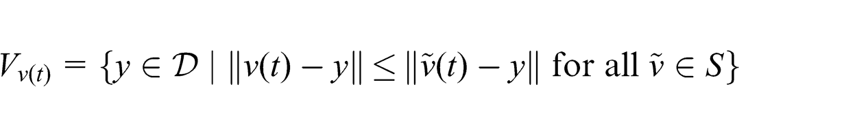
V_{v (t)} = {y \in D | ‖ v (t) - y ‖ \leq ‖ \tilde{v} (t) - y ‖ for all \tilde{v} \in S}

of all points in $D$ closest to sensor v at time t. The alpha complex A(t) is the nerve of the convex sets {B_v _(t)∩V_v(t)}_v ∈ S (Edelsbrunner and Mücke, 1994; Edelsbrunner and Harer, 2010). It is a subcomplex of both the $\overset{⌣}{C}$ ech complex and of the Delaunay triangulation, and is homotopy equivalent to the $\overset{⌣}{C}$ ech complex and to the union of the sensor balls. For points in general position the 1-skeleton of the alpha complex is embedded in the plane, although the 1-skeleton of the $\overset{⌣}{C}$ ech complex need not be. Recovering the alpha complex instead of the $\overset{⌣}{C}$ ech complex requires significantly stronger sensors. However, if each sensor measures the local distances to its overlapping neighbors, which may be approximated by time-of-flight, then this data determines the alpha complex (Fayed and Mouftah, 2009).

We assume there are only a finite number of times 0 < t₁ < … < t_n < 1 when the alpha complex changes. Hence for t and t′ in (t_i , t_i+1), [0, t₁), or (t_n , 1] we have identical alpha complexes A(t) = A(t′). Moreover, we assume that at each t_i one of the following changes to the alpha complex occurs.

A single edge is added or removed.

A single 2-simplex is added or removed.

A free pair consisting of a 2-simplex and a face edge with no other cofaces is added or removed.

A Delaunay edge flip occurs.

We assume that each sensor measures the clockwise cyclic ordering of its neighbors in the alpha complex. This cyclic ordering data is necessarily fixed in each interval (t_i , t_i+1), [0, t₁), or (t_n , 1].

Theorem 3. Suppose we have a planar sensor network with covered region X(t) connected at each time t ∈ I. Then from the time-varying alpha complex and the time-varying cyclic orderings of the neighbors about each sensor, we can determine whether or not an evasion path exists.

Proof. Let A ¹(t) be the 1-skeleton of the alpha complex at time t. For each vertex v we have a cyclic permutation π_v acting on the incident edges, where π_v (e) is the successor of edge e in the clockwise ordering around v. This gives A ¹(t) the structure of a rotation system (Mohar and Thomassen, 2001), also called a fat graph or ribbon graph (Igusa, 2002). A rotation system partitions the directed edges of A ¹(t) into sets of boundary cycles. Each boundary cycle is a loop of directed edges (e₁ e₂…e_k ) constructed so that if v_i is the target vertex of directed edge e_i , then $π_{v_{i}} (e_{i}) = e_{i + 1}$ , where e_k+1 = e₁. See Figure 15 for an example, and note that this cyclic ordering data distinguishes the two sensor networks in Figure 13.

The boundary cycles of A ¹(t) are in bijective correspondence with the connected components of $R^{2} ∖ A^{1} (t)$ . Removing the boundary cycles of length three that are filled by 2-simplices (and also the boundary cycle corresponding to the outside of $\partial D$ ) produces a bijection with the connected components of the uncovered region X(t)^c. Hence, by tracking the boundary cycles of A ¹(t) we can measure how the connected components of the uncovered region merge, split, appear, and disappear. In other words, we can reconstruct the Reeb graph of X^c →I (Reeb, 1946).

We will maintain labels on the boundary cycles of A ¹(t) so that a boundary cycle is labeled true if the corresponding connected component of $R^{2} ∖ A^{1} (t)$ may contain an intruder and false if not. At time t = 0 we label the boundary cycles of length three filled by 2-simplices in $A^{1} (0)$ (and also the boundary cycle corresponding to the outside of $\partial D$ ) as false. All other boundary cycles are labeled true. When we pass a time t_i when the alpha complex changes, we update the labels as follows.

If a single edge is added, then a single boundary cycle splits in two since X(t) is connected. Each new boundary cycle maintains the original label. If a single edge is removed, then two boundary cycles merge since X(t) remains connected, and the new cycle is labeled true if either of the original two cycles were labeled true.

If a single 2-simplex is added, then the label on the corresponding boundary cycle of length three is set to false. If a single 2-simplex is removed, then the label on the corresponding boundary cycle of length three remains false.

If a free pair consisting of a 2-simplex and a face edge is added, then a boundary cycle splits into two with one label unchanged. The other label corresponding to the added 2-simplex is set to false. If a free pair is removed, then the boundary cycle of length three corresponding to the 2-simplex is removed and the label on the other modified boundary cycle remains unchanged.

If a Delaunay edge flip occurs, then two boundary cycles labeled false are replaced by two different boundary cycles also labeled false.

An evasion path exists in the sensor network if and only if there is a boundary cycle in A ¹(1) labeled true. Such a boundary cycle corresponds to a connected component of the uncovered region X(1)^c at time one which could contain an intruder.□

Figure 16 shows that the connectedness assumption in Theorem 3 is necessary. It is an open question if the cyclic ordering information along with the time-varying $\overset{⌣}{C}$ ech complex (instead of the time-varying alpha complex) suffice.

Open Question. Suppose we have a planar sensor network with X(t) connected at each time t. Using only the time-varying $\overset{⌣}{C}$ ech complex and the time-varying cyclic orderings of the neighbors about each sensor, is it possible to determine whether an evasion path exists?

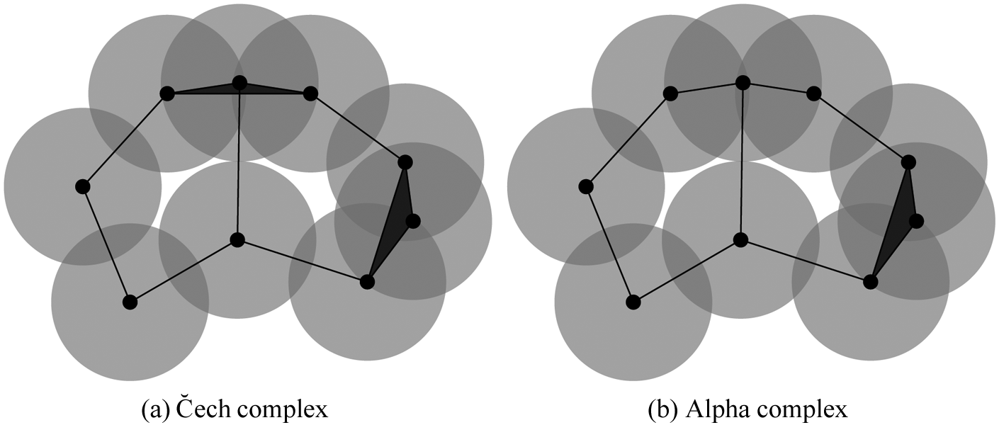
An answer to this open question would fill the gap between Theorem 7 of de Silva and Ghrist (2006) or equivalently our Theorem 2, which use only minimal sensor capabilities but are not sharp, and our Theorem 3, which is sharp but requires more advanced sensors measuring alpha complexes. One difficulty in working with the $\overset{⌣}{C}$ ech complex is that its 1-skeleton need not be embedded in the plane; see Figure 14(a).

Fig. 14.

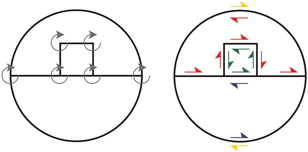
The alpha complex (b) is a homotopy equivalent subcomplex of the $\overset{⌣}{C}$ ech complex (a). For points in general position the 1-skeleton of the alpha complex is embedded in the plane, but the 1-skeleton of the $\overset{⌣}{C}$ ech complex need not be.

Fig. 15.

An example rotation system. The cyclic orderings are drawn on the left in gray, and the four boundary cycles are drawn on the right in red, green, blue, and yellow.

9. Conclusions

This paper addresses an evasion problem for mobile sensor networks in which the sensors do not know their locations and instead measure only local connectivity data. De Silva and Ghrist (2006) provide a homological criterion depending on this limited input which rules out the existence of an evasion path in many sensor networks. We use zigzag persistence to produce a criterion of equivalent discriminatory power that also allows for streaming computation, which is an important feature for sensor networks moving over a long period of time.

It turns out that no method relying on connectivity data alone can determine in all cases whether an evasion path exists. Indeed, we provide examples showing that the fibrewise homotopy type of the sensor network does not determine the existence of an evasion path; the embedding of the sensor network in spacetime also matters. We therefore consider a stronger model for planar sensors which measure cyclic orderings and alpha complexes, and given this model we provide necessary and sufficient conditions for the existence of an evasion path.

We end with two possible directions for future research. First, we are interested in the open question from Section 8: can one determine the existence of an evasion path using only $\overset{⌣}{C}$ ech complexes and the cyclic ordering data? An answer to this question would fill the gap between Theorem 7 of de Silva and Ghrist (2006) (or equivalently our Theorem 2) and our Theorem 3. Second, the evasion problem motivates a natural extension discussed in Adams (2013): can we describe the entire space of evasion paths? Knowledge about the space of evasion paths may be helpful in determining how to best patch a sensor network that contains an evasion path. Alternatively, we may want to find the evasion path that maintains the largest separation between the intruder and the sensors, that requires an intruder to move the shortest distance, or that requires an intruder to move at the lowest top speed. Knowledge about the space of sections may be helpful for such problems.

Footnotes

Appendix: C ⌣ ech complex approximations

In this appendix we explain the Vietoris–Rips approximation to the Cech complex. We still assume that each sensor covers a ball of radius one, but we now consider different communication distances between the sensors. Two sensors no longer detect when they overlap, but instead when their centers are within communication distance 2ϵ. Hence, the sensors measure a time-varying communication graph which at time t has an edge between sensors v and $\tilde{v}$ if $‖ v (t) - \tilde{v} (t) ‖ \leq 2 ϵ$ .

The Vietoris–Rips complex VR(t,ϵ) is the maximal simplicial complex built on top of the connectivity graph with communication distance 2ϵ at time t. Equivalently, a simplex is in VR(t,ϵ) when its diameter is at most 2ϵ (Vietoris, 1927). Note a simplex is included in VR(t,ϵ) when all its edges are in the connectivity graph, and so the Vietoris–Rips complex can be constructed from the connectivity graph. See Figure 17 for an example.

By changing the communication distance of the sensors, we can approximate the $\overset{⌣}{C}$ ech complex from either direction using a Vietoris–Rips complex. Jung’s theorem (Jung, 1901) implies

VR (t, \sqrt{\frac{d + 1}{2 d}}) \subset C (t) \subset VR (t, 1)

Let $p : VR (t, ϵ) \to R^{d}$ be the projection of the Vietoris–Rips complex into $R^{d}$ , mapping each simplex affinely to the convex hull of its vertices in $R^{d}$ . It follows from Jung’s theorem that if every continuous map $s : I \to D$ satisfies $s (t) \in p (VR (t, \sqrt{\frac{d + 1}{2 d}}))$ for some t, then there is no evasion path. Similarly, if there is a continuous map $s : I \to D$ with s(t) ∉p(VR(t,1)) for all t, then there is an evasion path. Hence, we can use the time-varying Vietoris–Rips complex to prove one-sided results about the existence of an evasion path. For example, when d = 2 the bound $VR (t, \sqrt{\frac{d + 1}{2 d}}) \subset C (t)$ is closely related to Lemma 1 of de Silva and Ghrist (2006), and is used to provide necessary conditions for the existence of an evasion path.

Funding

This work was supported by the National Science Foundation (grant numbers DMS 0905823 and DMS 0964242), the Air Force Office of Scientific Research (grant numbers FA9550-09-1-643 and FA9550-09-1-0531), and the National Institutes of Health (grant number I-U54-ca49145-01). H. Adams was supported by a Ric Weiland Graduate Fellowship at Stanford University and by the Institute for Mathematics and its Applications.

References

Adachi

(1993) Embeddings and Immersions (Translations of Mathematical Monographs, vol. 124). Providence, RI: American Mathematical Society.

Adams

(2013) Evasion paths in mobile sensor networks. PhD Thesis, Stanford University, USA. http://purl.stanford.edu/ys751yt6799.

Ahmed

Kanhere

Jha

(2005) The holes problem in wireless sensor networks: A survey. ACM SIGMOBILE Mobile Computing and Communications Review 9(2): 4–18.

Baryshnikov

Ghrist

(2009) Target enumeration via Euler characteristic integrals. SIAM Journal on Applied Mathematics 70(3): 825–844.

Carlsson

de Silva

(2010) Zigzag persistence. Foundations of Computational Mathematics 10(4): 367–405.

Carlsson

de Silva

Morozov

(2009) Zigzag persistent homology and real-valued functions. In: Proceedings of the 25th Annual Symposium on Computational Geometry. New York: ACM Press, pp. 247–256.

Chin

Dong

Hon

CYT

Yau

DKY

(2010) Detection of intelligent mobile target in a mobile sensor network. IEEE/ACM Transactions on Networking 18(1): 41–52.

Chung

Hollinger

Isler

(2011) Search and pursuit–evasion in mobile robotics. Autonomous Robots 31(4): 299–316.

Crabb

James

(1998) Fibrewise Homotopy Theory. London: Springer.

10.

de Silva

Ghrist

(2006) Coordinate-free coverage in sensor networks with controlled boundaries via homology. The International Journal of Robotics Research 25(12): 1205–1222.

11.

de Silva

Ghrist

(2007) Coverage in sensor networks via persistent homology. Algebraic and Geometric Topology 7: 339–358.

12.

de Silva

Morozov

Vejdemo-Johansson

(2011) Dualities in persistent (co)homology. Inverse Problems 27(12): 124003.

13.

Derksen

Weyman

(2005) Quiver representations. Notices of the American Mathematical Society 52(2): 200–206.

14.

Edelsbrunner

Harer

(2010) Computational Topology: An Introduction. Providence, RI: American Mathematical Society.

15.

Edelsbrunner

Letscher

Zomorodian

(2002) Topological persistence and simplification. Discrete and Computational Geometry 28(4): 511–533.

16.

Edelsbrunner

Mücke

(1994) Three-dimensional alpha shapes. ACM Transactions on Graphics 13(1): 43–72.

17.

Estrin

Culler

Pister

Sukhatme

(2002) Connecting the physical world with pervasive networks. IEEE Pervasive Computing 1(1): 59–69.

18.

Fan

Jin

(2010) Coverage problem in wireless sensor network: A survey. Journal of Networks 5(9): 1033–1040.

19.

Fayed

Mouftah

(2009) Localised alpha-shape computations for boundary recognition in sensor networks. Ad Hoc Networks 7(6): 1259–1269.

20.

Gabriel

(1972) Unzerlegbare darstellungen I. Manuscripta Mathematica 10(1): 71–103.

21.

Gao

Guibas

(2012) Geometric algorithms for sensor networks. Philosophical Transactions of the Royal Society A 370(1958): 27–51.

22.

Ghosh

Das

(2008) Coverage and connectivity issues in wireless sensor networks: A survey. Pervasive and Mobile Computing 4(3): 303–334.

23.

Ghrist

Lipsky

Poduri

Sukhatme

(2008) Surrounding nodes in coordinate-free networks. In: Algorithmic Foundation of Robotics VII. New York: Springer, pp. 409–424.

24.

Haefliger

(1961) Differentiable imbeddings. Bulletin of the American Mathematical Society 67(1): 109–112.

25.

Hatcher

(2002) Algebraic Topology. Cambridge: Cambridge University Press.

26.

Igusa

(2002) Higher Franz-Reidemeister Torsion (AMS/IP Studies in Advanced Mathematics, vol. 31). Providence, RI: American Mathematical Society.

27.

Jung

(1901) Über die kleinste Kugel die eine räumliche Figur einschliesst. Journal für die reine und angewandte Mathematik 123: 241–257.

28.

Kališnik

(2013) Alexander duality for parameterized homology. Homology, Homotopy and Applications 15(2): 227–243.

29.

Liu

Brass

Dousse

Nain

Towsley

(2005) Mobility improves coverage of sensor networks. In: Proceedings of the 6th ACM international symposium on mobile ad hoc networking and computing, pp. 300–308.

30.

Mac Lane

(1998) Categories for the Working Mathematician (Graduate Texts in Mathematics, vol. 5). New York: Springer.

31.

Mohar

Thomassen

(2001) Graphs on Surfaces (Johns Hopkins Studies in the Mathematical Sciences, vol. 2). Baltimore, MD: Johns Hopkins University Press.

32.

Reeb

(1946) Sur les points singuliers d’une forme de pfaff complèment intégrable ou d’une fonction numérique. Comptes Rendus de L’Académie ses Séances, Paris 222: 847–849.

33.

Vietoris

(1927) Über den höheren zusammenhang kompakter räume und eine klasse von zusammenhangstreuen abbildungen. Mathematische Annalen 97(1): 454–472.

34.

Wang

(2011) Coverage problems in sensor networks: A survey. ACM Computing Surveys 43(4): 32.

35.

Weiss

(1999) Embeddings from the point of view of immersion theory: Part I. Geometry and Topology 3: 67–101.

36.

Whitney

(1944) The self-intersections of a smooth n-manifold in 2n-space. The Annals of Mathematics 45(2): 220–246.

37.

Zomorodian

Carlsson

(2005) Computing persistent homology. Discrete and Computational Geometry 33(2): 249–274.