






Abstract
The semantic mapping of the environment requires simultaneous segmentation and categorization of the acquired stream of sensory information. The existing methods typically consider the semantic mapping as the final goal and differ in the number and types of considered semantic categories. We envision semantic understanding of the environment as an on-going process and seek representations which can be refined and adapted depending on the task and robot’s interaction with the environment. In this work we propose a novel and efficient method for semantic parsing, which can be adapted to the task at hand and enables localization of objects of interest in indoor environments. For basic mobility tasks we demonstrate how to obtain initial semantic segmentation of the scene into ground, structure, furniture and props categories which constitute the first level of hierarchy. Then, we propose a simple and efficient method for predicting locations of objects that based on their size afford a manipulation task. In our experiments we use the publicly available NYU V2 dataset and obtain better or comparable results than the state of the art at a fraction of the computational cost. We show the generalization of our approach on two more publicly available datasets.
1. Introduction
In recent years numerous advances have been made in semantic mapping of environments. It has been recognized that the capability of associating semantic concepts with geometric entities in robot’s surroundings can enhance robot’s autonomy and robustness, facilitate more complex tasks and enable better human–robot interaction. These observations led to a large number of approaches, which proposed varying numbers and types of semantic concepts and means of associating them with different parts of the environments. Examples of these included names of rooms/locations and various object and non-object categories. With the exception of a few approaches, semantic parsing at the basic level was formulated as a classification problem, where simple mapping between the sensory data and semantic concepts has been considered. In the proposed work we argue that semantic concepts are naturally arranged in a hierarchy and hierarchical categorization is often more suitable, both in terms of efficiency and adaptability for specific tasks. While in the context of lifelong learning it is desirable to be able to recognize a large number of object categories, it is not necessary to try to recognize them at all times. For example, for basic mobility tasks it is sufficient to be able to understand the free space, walls and obstacles, but it is not necessary to recognize a variety of objects in indoor environments. On the other hand, in the context of object search, more detailed categorization and localization is needed, if one were to facilitate ‘pick up and place’ tasks. In this work we demonstrate how to obtain initial semantic segmentation of the scene into ground, structure, furniture and props categories, which are commonly encountered in indoor environments. These categories along with the geometric features will constitute the first level of hierarchy. This initial semantic segmentation and confidences about presence of objects, will be followed by computation of additional features and generation of hypotheses for objects that based on their size afford a manipulation task.
1.1. Proposed approach
We formulate the semantic labeling problem in the conditional random field (CRF) framework, where the dependencies between random variables are represented by a graph, induced by both image superpixels and 3D scene structure. The distinguishing features of our approach are as follows. (a) The use of a tree graph structure in the CRF setting which effectively approximates the dependencies and enables exact and efficient inference amenable for real-time implementation. (b) The use of simple and efficient appearance and geometric cues, providing evidence about depth discontinuities. We carry out the semantic parsing experiments on the NYU V2 dataset (Silberman et al., 2012) 1 , which contains 464 diverse indoor scenes and 1449 annotated frames, achieving superior or comparable performance at the fraction of computational cost. We also show qualitative and quantitative results on the B3DO and UWobj datasets (Janoch et al., 2011; Lai et al., 2011). (c) We show how our system can be integrated with object detectors, in two ways: by pruning the set of candidate locations for less expensive feature computation, and by using the semantic classes’ probabilities outcome as a part of the feature vector.
In the next section, we provide an overview of the related work. In Sections 3 and 4 we describe the details of our approach. Section 5 describes the experiments on the NYU V2 dataset and compares our approach with the state-of-the-art methods. Finally, in Section 6 we present discussions and conclusions of the presented work and discuss possible future directions.
2. Related work
Previous approaches for semantic segmentation varied in the number and type of semantic concepts, means of associating them with different parts of the environments and computational models considered. Examples of the most commonly encountered semantic categories included the names of rooms or locations and various object and non-object categories. In the following section we mostly focus on the review of more recent methods which exploit both 3D geometric and appearance features computed from RGB-D sensors (e.g. Kinect) or obtained by 3D reconstruction.
In indoor environments several methods have been developed exploiting the RGB-D data. Koppula et al. (2011) highlighted the need for efficiency of the final inference and used up to 17 object classes. They were able to exploit stronger appearance and contextual cues due to the scale and different nature of the environment. Recently several researchers carried out more comprehensive experiments on the larger NYU RGB-D dataset introduced by Silberman and Fergus (2011). Ren et al. (2012) focused on local patch-based kernel features and achieved very good average performance while considering 13 structural and furniture classes and grouping all of the smaller objects into ‘other’ categories. The proposed features are computed over high-quality superpixels obtained with computationally expensive boundary detector (Martin et al., 2004). In addition to inference of semantic labels in the work of Silberman et al. (2012) the authors simultaneously considered the problem of inference of the support relations between different semantic categories. The approach relied on an elaborate pre-processing stage involving hierarchical segmentation stage, reasoning about occlusion boundaries and piecewise planar segmentation. All of these stages required a solution to a separate inference problem, using additional features and stage-specific energy functions. In the final inference problem the feature vectors computed over superpixels were over 1000 dimensions. A similar strategy is followed by Gupta et al. (2013) where the authors used the available depth information to improve the initial segmentation, followed by classification of obtained segments. In order to associate disconnected segments belonging to the same object category, they also proposed a long-range amodal completion to improve the segmentation consistency. The above-mentioned approaches relied on improvements of bottom-up segmentation using the depth data as additional cue, followed by classification of the obtained regions. Couprie et al. (2013) bypass the complex feature computation and segmentation stage and use convolutional networks for semantic segmentation. The final hypotheses are then evaluated on over-segmentation for the indoor scenes labeling task.
In contrast to our work the methods reviewed above consider the semantic segmentation as a final goal and are computationally expensive. The proposed approach infers the coarsest level of the semantic hierarchy which can be further refined based on the task.
Another class of approaches for semantic scene understanding focus on the problem of object detection, with or without the bottom-up segmentation stage. The framework based on sliding window object detectors has been explored by Sun et al. (2013) and Lai et al. (2012) using RGB-D sensors. In their work the objects are viewed in a table-top setting at moderate scale. The authors formulated the object detection problem as an inference on a voxel grid, reconstructed from multiple frames of RGB-D data. The final inference is carried in MRF framework, where the data term accumulates evidence from the sliding-window-based detectors trained on different views of the objects. A variant of the HOG descriptor (Lai et al., 2011) was used for capturing the appearance and shape information of each view of an object and trained using support vector machines (SVMs). The larger extent of the objects in the dataset (Lai et al., 2011) and sufficient number of training examples made the use of HOG based detector feasible. Another related work on unsupervised object discovery (Collet et al., 2011) has shown promising results for closer range and small amount of clutter. The work of Mishra et al. (2012) also considers the problem of detection of generic simple objects in an unsupervised setting, relying on the computation of the boundary using both RGB and depth data, followed by a selection of salient points and boundary completion. This methods is very effective for closer range table-top settings, where both depth discontinuities and support surfaces can be well estimated and the process of detection of image contours is more reliable. Their methods relies on a high-quality contour detector (Martin et al., 2004), which is quite expensive to compute. The generic object hypotheses proposed by this detector were then fed to a specific contour-based classifier using a so-called torque descriptor (Teo et al., 2013). The approaches which focus on object detection and categorization are suitable for close-range operation where the place that contains the objects has already been determined and the robot is only deciding which object to pick up.
Several approaches have been proposed for “objectness” detection using image-only information (Alexe et al., 2010; Carreira and Sminchisescu, 2010; Endres and Hoiem, 2010; Cheng et al., 2014). These approaches again are focused on object-centered images and, with the exception of Cheng et al. (2014), typically take of the order of seconds or even minutes to process every frame. In Section 5.2.2 we include comparisons with the recently proposed generic object detector (Cheng et al., 2014), which has shown better performance than similar image-only systems.
The above-cited works differ significantly in the nature of the datasets used to evaluate approaches to semantic segmentation and object detection. The most important distinguishing characteristic is the scale at which objects appear in images. For the datasets, where the objects appear in a table top setting, the challenges come from proper feature selection and efficient categorization in the presence of clutter. The datasets which contain more open scenes focus mostly on improvements in classification of non-object categories (Silberman et al., 2012; Couprie et al., 2013) and large objects appearing in the dataset (Gupta et al., 2013).
In our work we attempt to bridge methods which rely on semantic segmentation of open scenes with larger depth variation and table-top object detection. Instead of striving to achieve high accuracy of object detection for objects appearing at smaller scales in open scenes, we propose a representation and efficient framework which can be used for priming general object search and semantic understanding of non-object components of the environment.
Another line of work attempts to bring in the semantic information to the existing systems and approaches for simultaneous localization and mapping (SLAM). Häne et al. (2013) have proposed a batch algorithm for jointly segmenting the scene and optimize the 3D reconstruction. Their system is a very good option for post-processing but hardly applicable in online robotic operation. An online SLAM system recognizing objects is proposed by Civera et al. (2011), where in parallel to a monocular extended Kalman filter (EKF) SLAM thread there is a thread comparing visual features with the visual features of objects in the database. The recognition thread is always comparing against all of the specific instances and as such is not scalable in the number of different objects and instances. The approach of Salas-Moreno et al. (2013) solves the SLAM problem aided by the a priori knowledge of some objects. In real-time this SLAM system is able to recognize these objects and optimize their pose and the full map given the object models in the database. Although impressive in the results, this approach does not scale well with the number of different objects in the database and it is not suitable for the exploration of new environments or the discovery of new object instances.
In our approach we also strive to develop a framework which is efficient and amenable for real-time implementation. While efficiency has been considered extensively in the context of vision-based SLAM methods, the current techniques for semantic segmentation are computationally expensive and work predominantly in an off-line setting.
The complex issues of representation of semantic knowledge along with the spatial knowledge and the role of ontologies has been pointed out in the work of Pronobis et al. (2010). The authors focused more on exploiting the interplay between room locations and object identities, without considering more detailed semantic segmentation.
3. Semantic segmentation
We formulate the semantic parsing in the framework of CRFs with a tree graph structure encoding the pairwise relationships. We assume that an image and a 3D point cloud of the scene are available. Our approach starts by over-segmenting the image using the efficient simple linear iterative clustering (SLIC) algorithm (Achanta et al., 2012). Every superpixel in the image is interpreted as a cluster in the 3D point cloud for further computations. The 3D centroid of each cluster is used to compute a minimum spanning tree over Euclidean distances, defining the edges for the graphical model. The data and pairwise terms are determined using simple yet discriminative appearance and geometric cues for the classes that we are interested in. The learning and the final inference process are carried out over the graph in the CRFs framework. In the remainder of this section we detail the components of our approach and explain the intuition behind them.
3.1. Framework: CRFs
CRFs are probabilistic undirected graphical models first developed by Lafferty et al. (2001) for labeling sequence data. CRFs are a case of Markov random fields, and thus satisfy the Markov properties. Instead of relying on Bayes’ rule to estimate the distribution over hidden states
The nodes in a CRF are denoted
A CRF factorizes the conditional distribution into a product of potentials. We consider only the potentials for nodes ϕ(
where Z(
where [
3.2. Minimum spanning tree over 3D distances
Instead of computing the graph at the pixel level, we over-segment the image into superpixels. The CRF graph structure is typically determined by the neighborhood relations between superpixels. This often yields dense graph structure, see Figure 1(a), which is prone to over connect unrelated classes. We define the graph structure for the CRF as a minimum spanning tree over the Euclidean distances between 3D superpixel’s centroids in a scene. By definition, the minimum spanning tree connects points that are close in the measurement space, highlighting intrinsic locality in the scene, see Figure 1(b). This graph structure was already used in the context of object recognition (Quattoni et al., 2007) and place recognition (Cadena et al., 2012). Cadena et al. (2012) used it for graph matching for place recognition, where the nodes correspond to a sparse set of detected keypoints and the idea was to keep the structure of the graph between the matched nodes in a pair of scenes, while in the current work we handle a denser and structured 3D point cloud and we exploit that physical entities are continuous by nature.
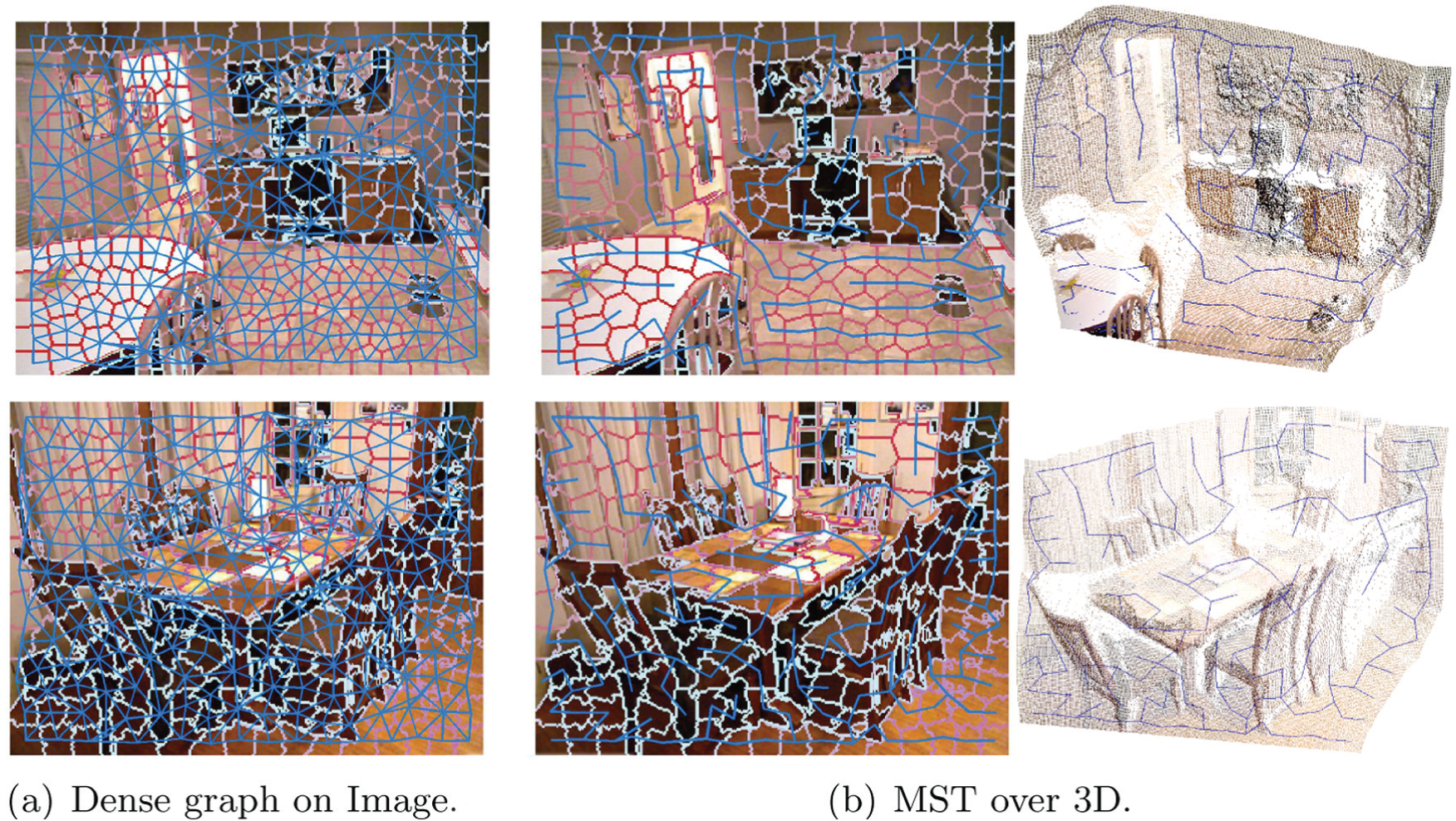
Graph Structures (blue lines). (a) The most common graph structure used in the computer vision community. (b) The graph structure selected by us, a minimum spanning tree over 3D euclidean distances.
Given that our graph structure is a tree we can use the belief propagation (sum-product) algorithm to exactly infer the marginal distribution of each node, and the max-product algorithm to find the MAP assignment (Koller and Friedman, 2009).
3.3. Feature description
With the graph structure defined for our CRF model, we have to define feature functions
where the local prior Ps(
where f(lj) (respectively
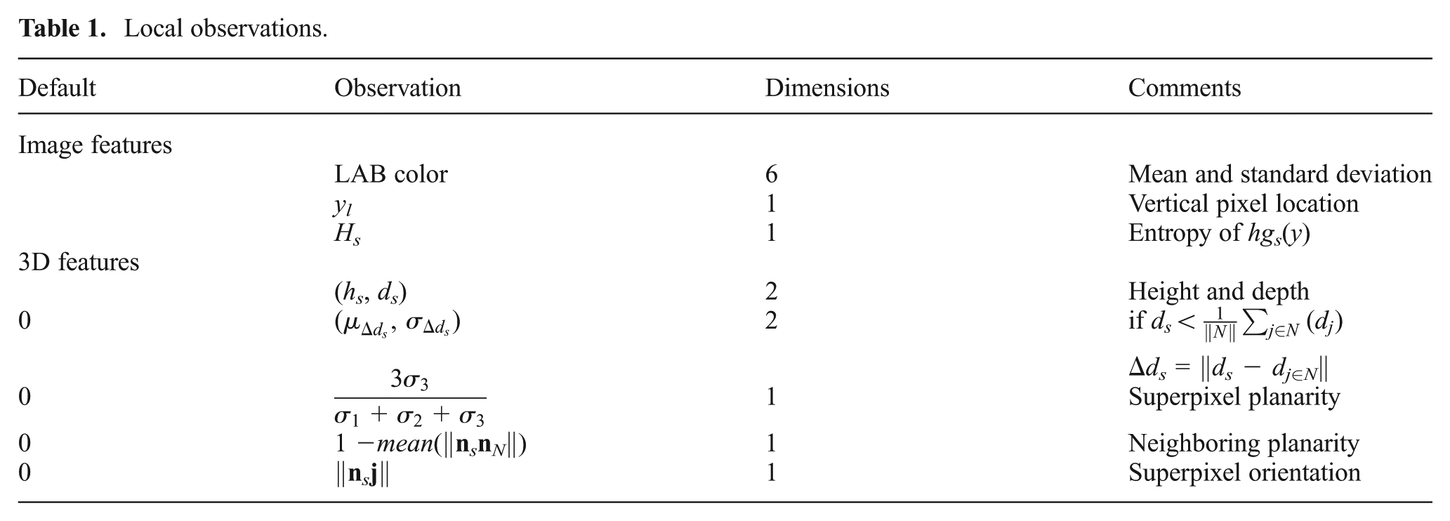
Local observations.
3.3.1. Image features
The mean and standard deviation of each channel in the LAB color space for the superpixel.
The vertical pixel coordinate for the superpixel’s centroid.
The entropy of the probability distribution for the superpixel boundaries belonging to the dominant vanishing directions in the scene, see Figure 2 rightmost.
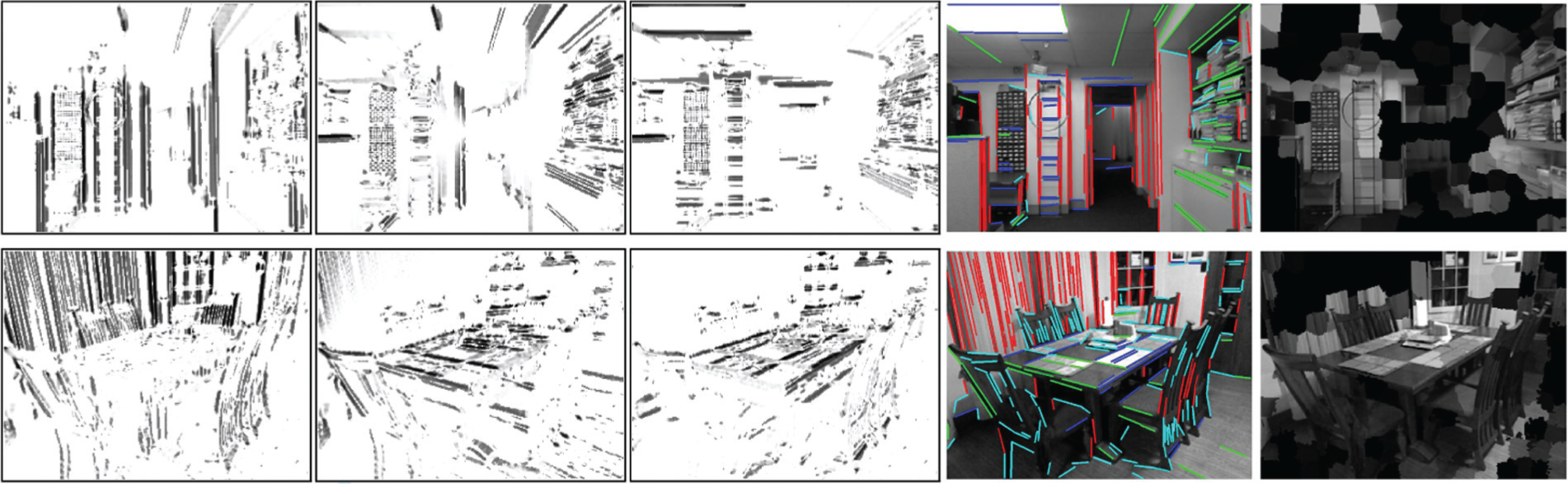
Gradient mixture model (Coughlan and Yuille, 2003). From the left: three gradient probability images of being aligned to each of three vanishing points, a color-coded membership image with lines to one of three vanishing points (red, green, blue), not to be consistent with any (cyan). Rightmost, the image with brightness proportional to the entropy of each superpixel.
The entropy feature expresses geometric consistency of a superpixel boundary with a particular vanishing direction. This feature is motivated by the observation that in indoor environments superpixel boundaries are often aligned with the vanishing directions. This observation has been also widely utilized in single-view reconstruction techniques (e.g. Hoiem et al., 2007). We employ a five-component gradient mixture model for the Manhattan world described in Coughlan and Yuille (2003). For each image pixel, the model provides the probability of the pixel lying on an edge, probability to pointing to each of the three vanishing points, see Figure 2, and the probability of being noise. We take into account only those pixels having the probability of being on an edge higher than being noise. For each of those points a maximum over last four probabilities is chosen as a membership of the point to either being consistent with one of the three vanishing points or not to be consistent with any, see the fourth column in Figure 2. For a particular superpixel s, we compute a normalized histogram hgs(y) with four bins y = {1,2,3,4} from memberships of all pixels lying along the superpixel boundary. In order to differentiate between clutter or small objects and structural classes we use the entropy of this normalized histogram,
3.3.2. 3D features
For the 3D point cloud computed with the depth information we use cues from the 3D position and planarity, for the superpixel itself and for the superpixel with respect to its neighborhood. The cues are as follows.
The depth (ds) and height (hs) for the superpixel’s centroid.
The mean and standard deviation of the absolute difference between the depth ds and the neighborhood’s depths: ||ds − dj∈N||. These are only computed if
The superpixel planarity encoded by the curvature of a superpixels’ point cloud (Klasing, 2010) using the singular value decomposition (SVD) and sort the singular values such that σ1 > σ2 > σ3.
The neighborhood planarity computed as one minus the mean of the dot product between the normal to the plane against to the neighborhood normals (Zhang et al., 2010).
The superpixel orientation, taken as the projection of the superpixel’s normal on the horizontal plane (Xiao and Quan, 2009).
The superpixel neighborhood N refers to all of the superpixels in contact with superpixel s in the image. In Table 1 we also show the default values and the dimensionality of these observations. As a result we compute for each superpixel 15-dimensional feature vector with 8 elements from image features and 7 from 3D features.
Pairwise term
The pairwise feature
where ||ci − cj||2 is the L2-norm of the difference between the mean colors of two superpixels in the LAB color space and l is the class label.
Given the graph structure and the features outlined above, we proceed with the description of the learning and inference stage and the performance evaluation of the final semantic segmentation approach in Section 5. An example of the probability distribution outcome from our approach is shown in Figure 3.

Exact marginals obtained with the sum-product algorithm. From the left: probability to be ground, structure, furniture and props. Darker means higher probability.
4. Priming object detection
In this section we show how the marginals from the semantic segmentation approach can be used in the task of localizing objects in the scene. We propose a simple detector for generic objects and show how to combine it with the semantic segmentation results to improve the detection rate and computational cost. Instead of training an object detector separately for each object category we consider a single category of generic objects whose extent can be well approximated by a bounding box. Each bounding box is then characterized by a boundary feature characterizing the orientation of the boundary close to the bounding box border. The feature is motivated by previous works on saliency and detection of generic objects (Alexe et al., 2010) and works for objects of relatively simple shape, where majority of the true object boundary is close to the bounding box boundary. In the next section we describe in more detail the boundary feature, the generic object detector and the method for proposing and scoring of candidate bounding boxes to generate object hypotheses.
4.1. Features and classifier
We compute the gradient orientations in four blocks depicted in Figure 4(right), obtained by shrinking and enlarging the bounding box by five pixels each, to capture the variation around the actual boundary. In each block we quantize the orientations from 0 to 360° into nine orientation bins. This is done both for intensity and depth channel yielding a 2 × 4 × 9 = 72-dimensional feature.
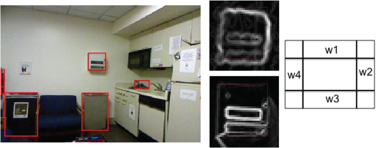
Examples of objects and their bounding boxes and close-up of the orientation energy for both intensity and depth channel. Center: orientation energy for paper towel dispenser, where the depth gradients and image gradients complement each other well. Right: window blocks in the vicinity of the boundary where the histograms are computed.
At this point we can introduce the first modification to include the semantic segmentation information into the feature vector. We compute the probability distribution of the bounding box over the four classes (ground, structure, furniture, props), by averaging and re-normalizing the pixel’s probabilities inside the window. Now, the feature vector is augmented with the four values resulting in a 76-dimensional feature vector.
We train an SVM classifier with histogram intersection kernel (Maji et al., 2008) using the mentioned feature vector. The positive examples come from the ground truth bounding boxes and the negative ones are randomly picked from the generated windows using the proposal of Van de Sande et al. (2011). In the window generation method of Van de Sande et al. (2011) the image is first over-segmented into superpixels, which are then merged using the criteria of similarity over the color space and superpixels’ sizes building a fine-to-coarse hierarchical over-segmentation. The bounding boxes of each superpixel at different levels in the hierarchy are possible candidates.
The ground truth is constrained to those objects with sides smaller that 50 cm and greater than 5 cm. We obtain the metric dimensions of the bounding boxes directly from the depth map. The negative examples are constrained by the same rule.
4.2. Object search strategy
At the test time, instead of generating candidate windows with different predefined aspect ratios and scales, we again use the strategy of Van de Sande et al. (2011) with the same constraints on the size as before.
Now, we introduce the second modification which is sampling the candidate windows with the probability of the bounding box belonging to furniture or props. The idea behind this sampling strategy is that if our semantic segmentation is confident that one candidate box covers the wall or the floor we do not need to evaluate the classifier on it or compute the features for that window. On the other hand, it is highly probable the objects we are looking for lie over furniture pieces or belong to the props semantic class.
5. Experiments
In our experiments we use the NYU V2 RGB-D dataset (Silberman et al., 2012), which contains 1449 labeled frames. The labeling spans over 894 different classes produced using Amazon Mechanical Turk. The authors of the dataset also provide a train and test splits and a mapping from the 894 categories to 4 classes: ground, structure, furniture and props, as was used by Silberman et al. (2012). We take 795 training frames for building the kd-tree and for CRF parameter learning, and the remaining 654 frames for testing and quantitative comparison against state-of-the-art methods in RGB-D semantic segmentation. 2
We obtain superpixel segmentation using the SLIC implementation from the VLFeat library of Vedaldi and Fulkerson (2008), followed by the computation of the features described in Table 1. With the computed features in the training set we build a kd-tree using the implementation of Buchanan and Fitzgibbon (2006) with the default parameters. Then for every superpixel in the training set we obtain the k-NN classification for the training data using Equation (4) with the k = 10 nearest neighbors.
The minimum-weight spanning tree (MST) is computed from 3D centroids of all of the superpixels. Now, using the MST graph, the output of the k-NN classifier in Equation (3) and the pairwise potentials (Equation (6)) we learn the parameters in the CRF setting. For the learning, inference and decoding with CRFs we use the Matlab code for undirected graphical models (UGM). 3
5.1. Results on semantic segmentation
At testing time, to obtain the most likely label assignment for the superpixels we solve the MAP problem over the CRFs. This problem does not require any threshold selection and all of the parameters are computed/learned from the data. The inference results give us the labeling assignments over superpixels, we transfer those to every pixel in the superpixel to compute the pixel-wise accuracy of semantic labeling. In Figure 5 we show several examples of the output of our approach.

Original images, ground truth labeling and MAP result from our approach in the NYU dataset.
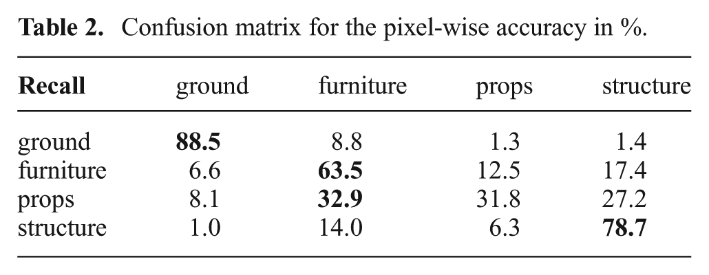
Table 2 shows the confusion matrix normalized by rows (recall on the diagonal). The props class is the most frequently confused. Props class is defined by Silberman et al. (2012) as “small objects that can be easily carried”. We can observe in the results (Figure 5) several planar objects (posters, carpets, placemats) are labeled as structure or furniture. Another source of confusion is due to the quality of the ground truth, where we found several ambiguities in the structure and furniture categories, where kitchen tables, stoves, dishwashers and cabinets were labeled as the two interchangeably.
Confusion matrix for the pixel-wise accuracy in %.
In first row of Table 3 we show the pixel-wise recall accuracy along with the average and global accuracy for our approach: CRF-MST and k-NN + SLIC with Image and 3D features. To study the importance of Image features versus 3D features, we remove one set at a time keeping the rest of the system intact. The rows Image features and 3D features show the corresponding performance when using only one type of features. Using only 3D features we can see better results for three out of four classes at the cost of very poor accuracy in props and smaller average and global accuracy. Our full system, with both sets of features obtains the best trade off for all performance measures. In Table 3 we also show the result by only using the data term, k-NN row, using the image and 3D information. It is clear that the MST and the CRF framework improve the general performance.
Pixel-wise percentage recall accuracy.
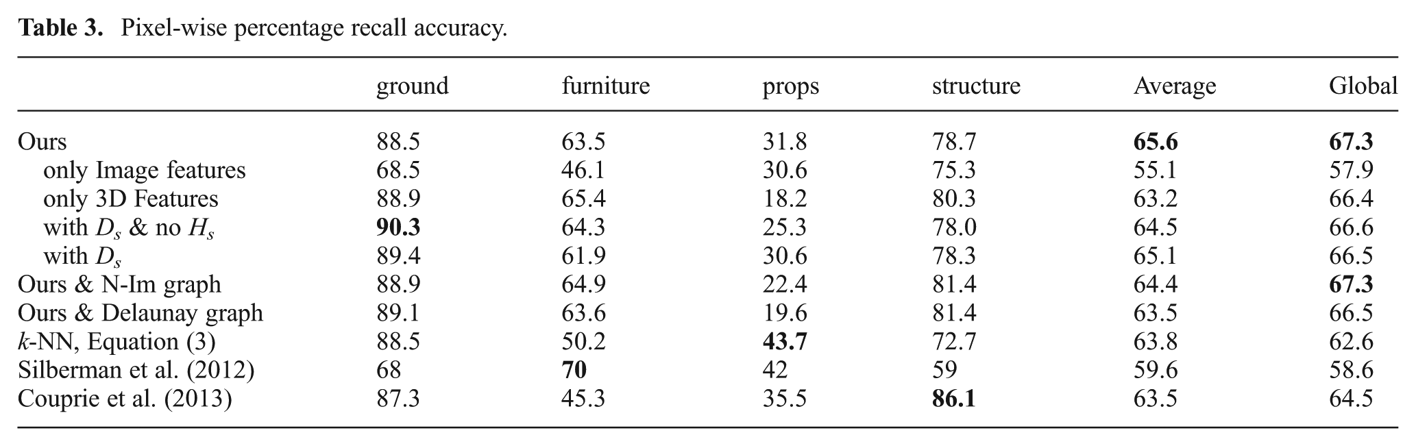
We have evaluated our system removing Hs from our features and adding Ds instead, and also using both, i.e. our features and Ds, (with Ds & no Hs) and (with Ds) in Table 3, respectively. In the first case the accuracy for ground is improved but for props is hurt. The second case, the performance for props improves again but in general is not as good as our initial proposal.
In comparison with the original work of authors who released this dataset (Silberman et al., 2012), as shown in Table 3, their system still obtains the best accuracy in the furniture and props classes. They use a feature vector of 1128 elements to compute the data term with a logistic regression classifier. The cues come from color (36), shape (1086) and scene (6) information (see the supplementary material in Silberman et al. (2012)). Our representation and features are notably simpler enabling more efficient feature computation and inference while still achieving comparable performance.
5.1.1. Independent datasets
We evaluate our semantic segmentation on two independent datasets: the Berkeley 3-D Object Dataset (B3DO) (Janoch et al., 2011) and the RGB-D Object Dataset from University of Washington (UWobj) (Lai et al., 2011). B3DO with 849 frames has more variability in the indoors scenes and spans from offices to house rooms. The smoothed depth information is obtained by another in-painting technique, different from that used by NYU V2. UWobj is a dataset that focuses on close-range object instance detection and object categorization and contains mostly table-top scenes from the lab with large extent objects. This dataset is released without in-painting in the depth maps. From both datasets we evaluate our semantic segmentation approach on the scenes that correspond to open space, instead to table-top scenes, as our semantic segmentation focuses on semantic classes relevant during navigation or exploration rather than for manipulation. We consider an open space any scene where the median of the depth map is greater than 2.5 meters leaving us with 182 frames from B3DO and 45 frames from UWobj. Some result are shown in Figure 6, we can see a similar performance that for the NYU V2 dataset, even with the differences in depth pre-processing, type of scenes and poses of the sensor, which show that our proposal is a general and powerful tool for semantic segmentation.
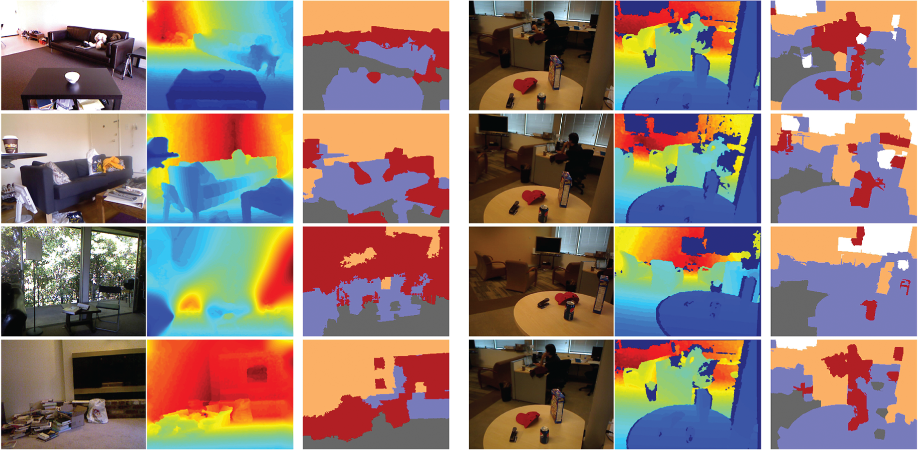
Original images, depth and MAP results from our approach in B3DO (Janoch et al., 2011) (left) and UWobj (Lai et al., 2011) datasets (right).
5.1.2. Timing
The experiments were carried out with a research implementation of our approach in Matlab. The computational cost, for NYU V2 in testing, is detailed in Figure 7, excluding the superpixel over-segmentation. The system runs on average at 1 fps in a single-thread of a 3.4 GHz IntelCore i7-2600 CPU M350 and 7.8 GB of RAM. Including the SLIC over-segmentation is still able to run at 0.5 fps. For the whole system, the mean and the maximum computational times are 0.7 and 1.0s, respectively. The average cost to obtain the SLIC superpixels is 611 ms, although a C++ implementation would take half of that time as reported by Achanta et al. (2012). In the feature computation the main bottleneck is the computation of the gradient mixture model (Coughlan and Yuille, 2003) for vanishing directions. The training stage takes less than 2 seconds to build the kd-tree and 180 seconds for the CRF parameter learning. In total including the feature computation, the computational cost for all of the training data is less than 20 minutes.
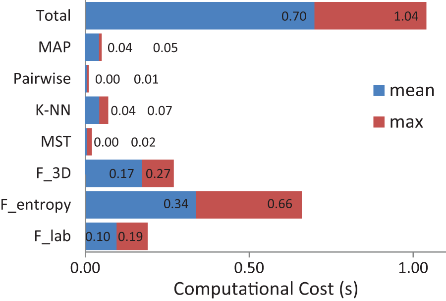
Detailed mean and maximum computational timing of 654 NYU V2 frames in testing excluding SLIC over-segmentation cost.
An initial implementation of semantic segmentation approach in C++ and using the GPU implementation of SLIC (gSLIC) of Ren and Reid (2011) is closer to a real-time operation working at around 5 fps. Table 4 shows the mean timing for both versions, Matlab/mex and C++/GPU. A more efficient system is possible by implementing other stages, e.g. k-NN, on the GPU.
Mean computational timing for the semantic segmentation system in milliseconds in the NYU-V2 test set.

5.2. Object localization
We train the object detector as described in Section 4 on the training set of the NYU V2 dataset and evaluate it on the test set from the same dataset and on B3DO and UWobj datasets. Figure 8 shows some example results from testing in all of the datasets.
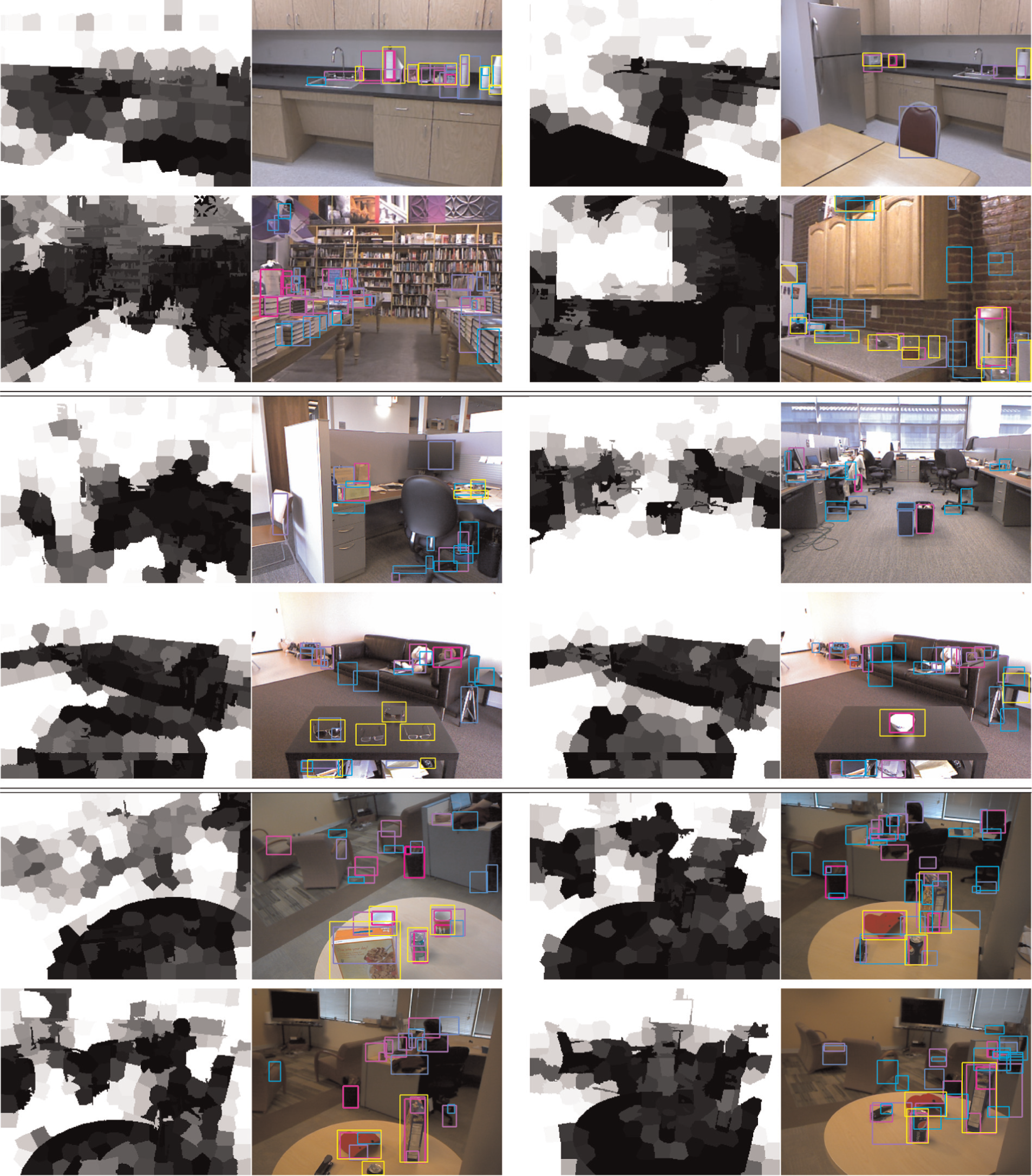
Priming object detection. The probability map, p(furniture) + p(props), for the sampling of candidates is on the left of every pair, darker means higher probability. On the right the image with ground truth bounding boxes (yellow) and detections. The color of the detection windows goes from cyan to pink as the SVM score increases. We show four examples for every dataset, NYU V2 (top), B3DO (middle) and UWobj (bottom).
We use the intersection over union measure greater than 0.5 to accept a detection (Everingham et al., 2010). We also use the concept of ground truth bounding boxes to ignore (BBGT−ig) as proposed by Dollár et al. (2012). Any proposal matched to a BBGT−ig does not count as good detection or as a false positive. This solves issues for example when we detect individual instances of objects and the BBGT−ig is covering a group of objects (book versus books).
5.2.1. Performance evaluation
In Figure 9 we show the performance of our approach for priming object detection in terms of F1-score versus detector SVM score, the SVM score is calibrated to span from 0 to 1. In order to show the contribution of using the semantic segmentation information we present three versions for our system, as described in Sections 4.1 and 4.2.
Ours [I, D], No sampling: This is the basic system, descriptor with intensity and depth channels without using the results from the semantic segmentation in any stage.
Ours [I, D, P], No sampling: Here we augment the descriptor with the probabilities from the semantic segmentation.
Ours [I, D, P], Sampling: Here we sample the bounding boxes proposals by p(furniture) + p(props) and augment the descriptor with the probabilities from the semantic segmentation.
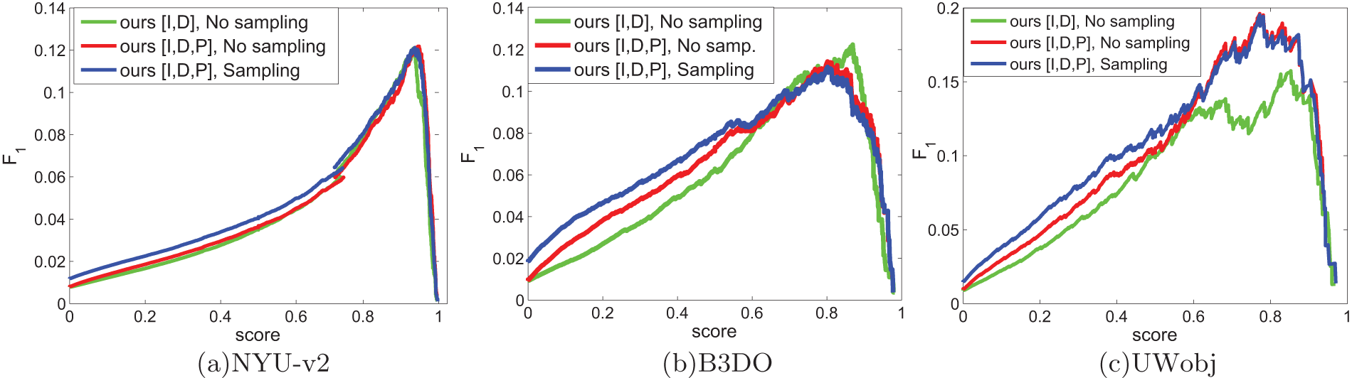
Comparison of F1-score versus detector SVM score when using the feature vector composed only by the intensity and depth information (ours [I, D]), when augmented by the semantic segmentation probability (ours [I, D, P]) and when pruning the candidate windows with the sampling proposed.
The F1-score curve shows how we improve the baseline system, first by augmenting the descriptor with the probabilities from the semantic segmentation and then by sampling using the p(furniture) + p(props). When setting a robotic system for real operation, we may determine a threshold for the SVM score, Figure 9 depicts that after choosing a threshold on one of the datasets the rank of the three versions is maintained to new environments. The major benefit in the sampling is reflected in the computational cost given the number of discarded candidates before the feature computation. For example, in Figure 10(left), without sampling, the cost for feature computation and SVM evaluation is 760 and 60 ms, respectively. Instead, with the sampling, Figure 10(right), the cost is 440 and 20ms. In Figure 11 we show the frequency of speed-up for all of the datasets. In the worst case there is almost no gain in efficiency in cluttered scenes, and in other scenes (e.g. corridors) we can get speed-ups of up to a factor of four.
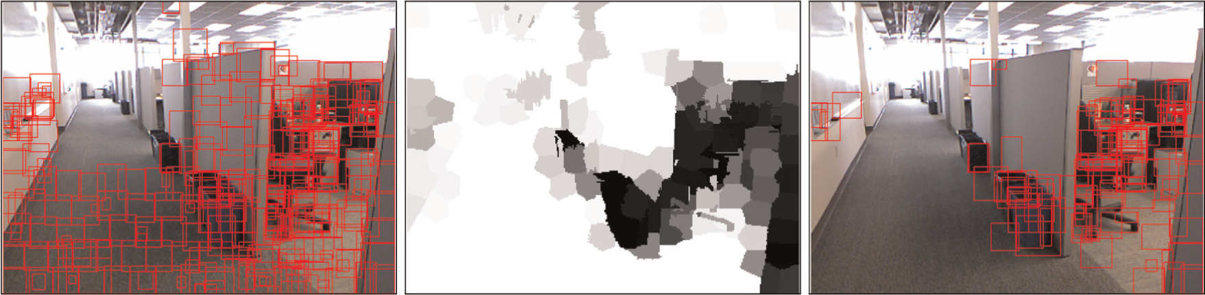
On the left all of the candidates, on the right the candidates after pruning by the probability of the window to be furniture or props shown in the middle (darker indicates higher probability).
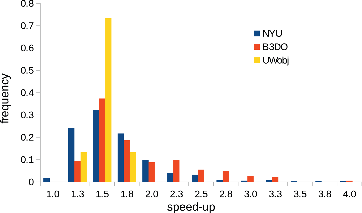
Frequency of speed-up for all datasets when using sampling driven by p(props) + p(furniture).
The low F1-scores for the object detector are due to the high proportion of false alarms. We can see in Figure 8 that we obtain several false alarms, but a lot of them are because the ground truth bounding boxes are incomplete and many objects which we successfully detect are not labeled at all. This problem is easy to find in the research community as the labeling is generated only for the specific objects of interest in each paper. However, in real-life applications a robot can find a possibly unlimited number of different objects and instances.
5.2.2. Comparisons
As a comparison with the state-of-the-art object detectors we include the results from the very recent BInarized Normed Gradients (BING) objectness estimation (Cheng et al., 2014). The source code is provided by the authors with a training on the PASCAL-VOC 2007 dataset. In Figures 12, 13 and 14, we depict the performance of the BING detector and of our approach in terms of detection rate (DR) versus false positives per image (fppi) and precision–recall (PR) curves. The DR-fppi and PR curves show that our object proposal system is better than the only-image state of the art. In the UWobj dataset BING is better than ours in one portion of the curve, if more than 50 fppi are allowed in a real system, and the reason for this is that this dataset is the most structured one among the three datasets, with objects in table-top setting and in the center of the image.
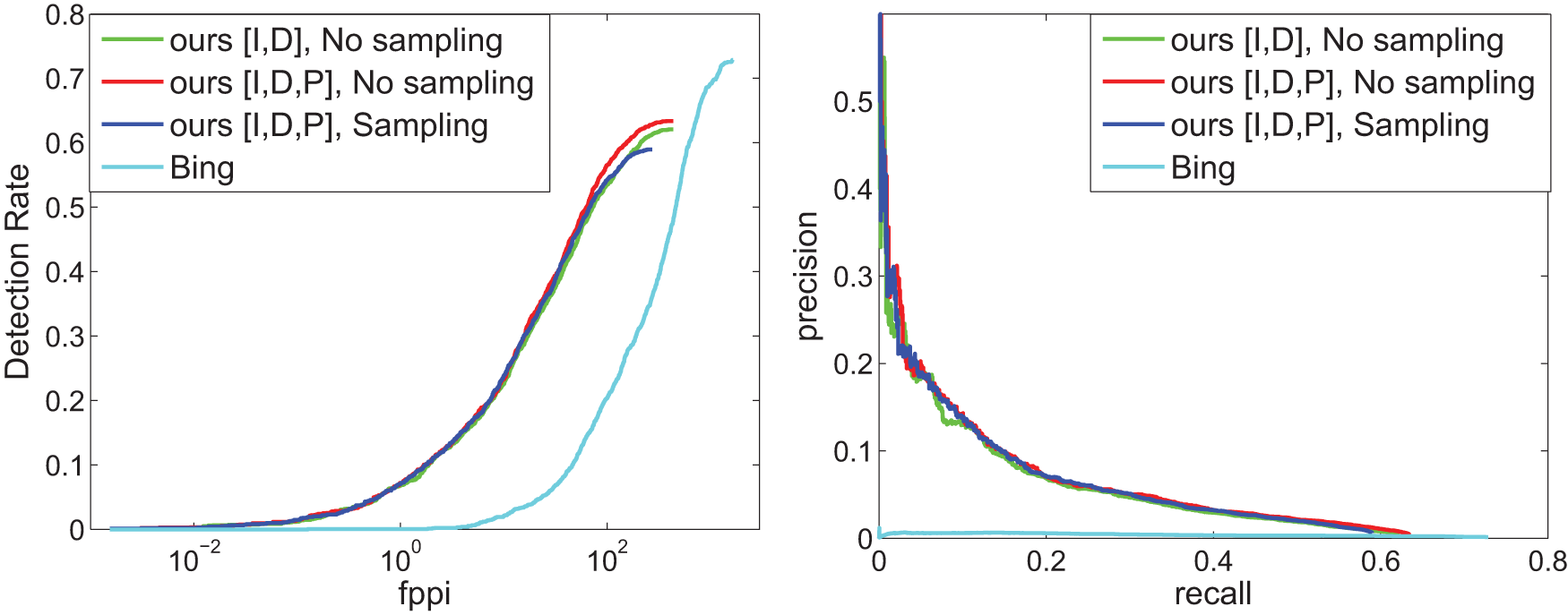
NYU-V2 dataset. Left: Detection rate versus false positives per image. Right: Precision versus recall.
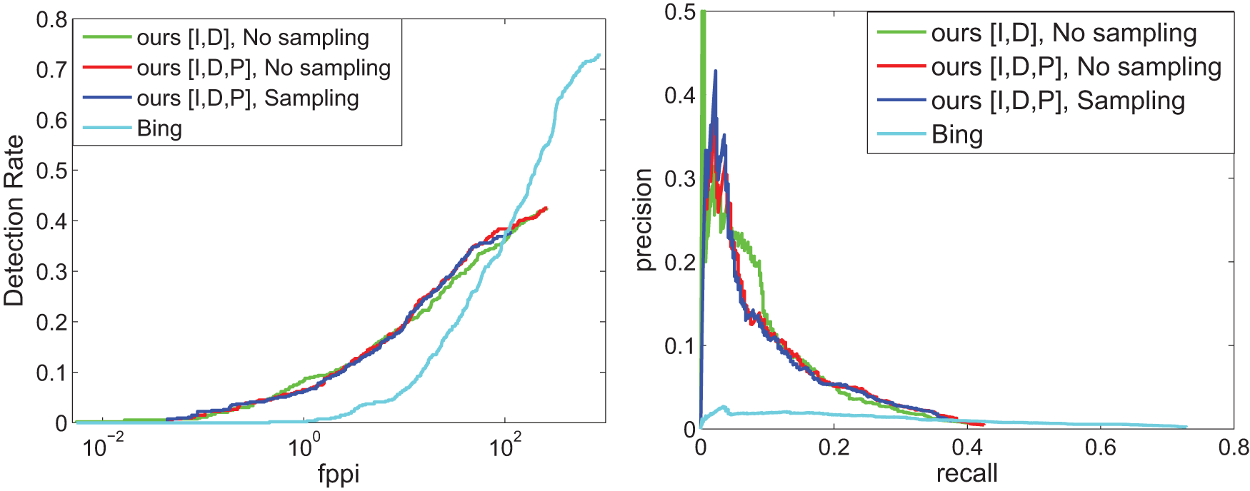
B3DO dataset. Left: Detection rate versus false positives per image. Right: Precision versus recall.
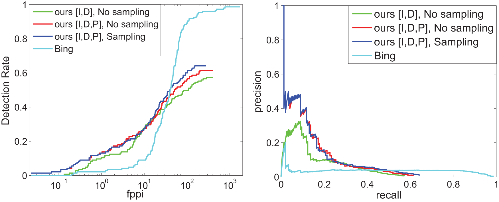
UWobj dataset. Left: Detection rate versus false positives per image. Right: Precision versus recall.
6. Discussion
We have shown a basic implementation with real-time capabilities that effectively uses appearance and 3D cues to generate evidence about the structure of the scene, while achieving better average and global accuracy of semantic labeling compared with the state of the art. Note that the accuracy reported by Couprie et al. (2013) was computed after training the system for 849 different classes and, then, the results were clustered into the four categories, indicating that their approach and features are less robust to the high intra-class variability in the four class problem.
We have shown that our graph structure induced by the MST over metric euclidean distances does not sacrifice the labeling accuracy, and keeps the intra-class components coherently connected. Furthermore, by this selection we gain an exact and efficient inference. The computational complexity for the inference is
An interesting discussion is related to the choice of basic representation and the features. Silberman et al. (2012) use over 1000-dimensional feature vectors, concatenating many engineered features, most of them developed previously for diverse but related tasks. On the other hand, Farabet et al. (2013) propose to avoid the feature engineering and learn the features from the data using convolutional networks. They are still using a 768-dimensional feature vector for RGB channels, and the feature vectors have over 1000 dimensions when including the depth channel (Couprie et al., 2013). We can see that in both approaches, feature engineering vs feature learning, high dimensional feature space is constructed in which the different classes are more easily separable. In this work we propose and demonstrate, that fewer (15-dimensional) but more meaningful features are sufficient to obtain better semantic segmentation in RGB-D scenes. In addition to the choice of features there are at least two more reasons for this improvement. First, selecting a well-performing local classifier to handle high intra-class variability: k-NN in our case versus logistic regression (Silberman et al., 2012), versus a two-layer multi-perceptron (Couprie et al., 2013). Second, defining a more natural connection between neighbors given the type of data: MST over 3D distances in our system, versus connecting all of the neighbors in the image (Silberman et al., 2012), versus no connections at all between superpixels (Couprie et al., 2013). Farabet et al. (2013) show a similar comparison.
We have also shown how to integrate the results of semantic segmentation with object detection, proposing a simple detector of generic objects whose shape can be well approximated by a bounding box. The performance of the object detection in terms of precision recall is not on a par with other object detection results where large objects and more discriminative features are considered (Ren et al., 2012). This is partly due to the lack of correctly labeled objects in the dataset (many small objects are part of the background class) and simplistic boundary feature descriptors. More sophisticated descriptors (e.g. Teo et al., 2013) and more accurate labeling can significantly improve the proposed approach.
We plan to explore strategies for obtaining the observations in a multi-scale way to improve the performance, this is inspired on the boosting achieved by Farabet et al. (2013) when comparing the multi-scale versus one-scale convolutional networks.
We expect a C++/GPU implementation for our object detection to work at more than 10 fps, a similar gain as for our semantic segmentation. Note that the BING detector (Cheng et al., 2014) works with image information only, and it is still possible to get a better performance by adapting it to take into account the depth channel, and maybe the semantic class probabilities, although a reduction in its efficiency is expected.
Footnotes
Funding
This research has been funded by the US Army Research Office (grant number W911NF-1110476) and the Australian Research Council (grant number DP130104413).