BRVO: Predicting pedestrian trajectories using velocity-space reasoning

Abstract

We introduce a novel, online method to predict pedestrian trajectories using agent-based velocity-space reasoning for improved human–robot interaction and collision-free navigation. Our formulation uses velocity obstacles to model the trajectory of each moving pedestrian in a robot’s environment and improves the motion model by adaptively learning relevant parameters based on sensor data. The resulting motion model for each agent is computed using statistical inferencing techniques, including a combination of ensemble Kalman filters and a maximum-likelihood estimation algorithm. This allows a robot to learn individual motion parameters for every agent in the scene at interactive rates. We highlight the performance of our motion prediction method in real-world crowded scenarios, compare its performance with prior techniques, and demonstrate the improved accuracy of the predicted trajectories. We also adapt our approach for collision-free robot navigation among pedestrians based on noisy data and highlight the results in our simulator.

Keywords

Trajectory prediction multi-agent simulation collision avoidance

1. Introduction

Robots are becoming increasingly common in everyday life. As more robots are introduced into human surroundings, it becomes increasingly important to develop safe and reliable techniques for human–robot interaction. Robots working around humans must be able to successfully navigate to their goal positions in dynamic environments with multiple people moving around them. A robot in a dynamic environment thus needs the ability to sense, track, and predict the position of all people moving in its workspace to navigate complicated environments without collisions.

Sensing and tracking the position of moving humans has been studied in robotics and computer vision, e.g. Rodriguez et al. (2009), Luber et al. (2010), and Kratz and Nishino (2011). These methods often depend upon an a priori motion model fitted for the scenario in question. However, such motion priors are typically based on globally optimized parameters for all the trajectories during the entire sequence of data, rather than only taking into account the specific individual’s movements. As a result, current motion models are not able to accurately capture or predict the trajectory of each pedestrian. For example, we frequently observe atypical pedestrian motion, such as moving against the flow of other agents in a crowd, or quick velocity changes to avoid collisions. In order to address these issues, many pedestrian tracking algorithms use multi-agent or crowd motion models based on local collision avoidance (Pellegrini et al., 2009; Yamaguchi et al., 2011). These multi-agent interaction models effectively capture short-term deviations from goal-directed paths, but in order to do so, they must already know each pedestrian’s destination; they often use handpicked destination information, or other heuristics that require prior knowledge about the environment. As a result, these techniques have many limitations: they are unable to account for unknown environments with multiple destinations, or times when pedestrians take long detours or make unexpected stops. In general, the assumption that the destination information remains constant can often result in large errors in predicted trajectories. Moreover, environmental factors, such as static or dynamic obstacles, dense crowds, and social/cultural behavior rules, make predicting the behavior or movement of each individual pedestrian more complicated, thereby making it more difficult to compute a motion from a single destination.

In this work, we seek to overcome these limitations by presenting a novel online prediction method (Bayesian reciprocal velocity obstacles, or BRVO) that is built on agent-based, velocity-space reasoning combined with Bayesian statistical inference; BRVO can provide an individualized motion model for each agent in a robot’s environment. Our approach models each pedestrian’s motion with their own unique characteristics, while also taking into account interactions with other pedestrians. This can be contrasted with the previous methods that use general motion priors or simple motion models. Moreover, our formulation is capable of dynamically adjusting the motion model for each individual in the presence of sensor noise and model uncertainty. We address the problems associated with fixed destination by integrating learning into our predictive framework and by adjusting short-term steering information.

Our approach works as follows. We generalize the problem by assuming that at any given time the robot has past observations for each person in the environment and wants to predict agent motion in the next several time steps (i.e. to aid in navigation or planning tasks). We apply ensemble Kalman filtering (EnKF) to estimate the parameters for a human motion model based on reciprocal velocity obstacles (RVO) (Van den Berg et al., 2008a, 2011). We use this combination of filtering and parameter estimation in crowded environments to infer the most likely state for each observed person: its position, velocity, and goal velocity. Based on the estimated parameters, we can predict the trajectory of each person in the environment, as well as their goal position. Our experiments with real-world pedestrian datasets demonstrate that our online per-agent learning method generates more accurate motion predictions than prior methods, especially for complex scenarios with noisy, low-resolution sensors, and missing data. Using our model, we also present an algorithm to compute collision-free trajectories for robots, which takes into account kinematic constraints; our approach can compute these paths at interactive rates in scenarios with dozens of pedestrians.

The rest of our paper is organized as follows. Section 2 reviews related work. Section 3 provides an overview of motion-prediction methods and the RVO crowd simulation method. Section 4 describes how our approach combines an adaptive machine-learning framework with RVO, and Section 5 presents our empirical results using real-world (video-recorded) data, along with analysis on these results. Section 6 presents a method to integrate our pedestrian prediction approach with modern mobile robot navigation techniques to improve collision avoidance for robots navigating in environments with moving pedestrians.

2. Related work

In this section, we give an overview of prior work on motion models in robotics and crowd simulation and on their applications to pedestrian tracking and robot navigation.

2.1. Motion models

There is an extensive body of work in robotics, multi-agent systems, crowd simulation, and computer vision on modeling pedestrians’ motion in crowded environments. Here we provide a brief review of some recent work in this field. Many motion models have come from the fields of pedestrian dynamics and crowd simulation (Pelechano et al., 2008; Schadschneider et al., 2009). These models are broadly classifiable into a few main categories: potential-based models, which models virtual agents in a crowd as particles with potentials and forces (Helbing and Molnar, 1995); boid-like approaches, which create simple rules to steer agents (Reynolds, 1999); geometric models, which compute collision-free velocities (Van den Berg et al., 2008b, 2011); and field-based methods, which generate fields based on continuum theory or fluid models (Treuille et al., 2006). Among these approaches, velocity-based motion models (Van den Berg et al., 2008b; Karamouzas et al., 2009; Pettré et al., 2009; Karamouzas and Overmars, 2010; Van den Berg et al., 2011) have been successfully applied to the simulation and analysis of crowd behavior and to multi-robot coordination (Snape et al., 2011); velocity-based models have also been shown to have efficient implementations that closely match real human paths (Guy et al., 2010).

2.2. People-tracking with motion models

Much of the previous work in people-tracking, including Fod et al. (2002), Schulz et al. (2003), and Cui et al. (2005), attempts to improve tracking quality by making simple assumptions about pedestrian motion. In recent years, robotics and computer vision literature have developed more sophisticated pedestrian motion models. For example, long-term motion-planning models have been proposed to combine with tracking. Bruce and Gordon (2004) and Gong et al. (2011) propose methods to first estimate pedestrians’ destinations and then predict their motions along the path towards the estimated goal positions. Liao et al. (2003) propose a method to extract a Voronoi graph from the environment and predict people’s motion along the edges, following the topological shape of the environment. Methods that use short-term motion models for people-tracking are also an active area of development. Luber et al. (2010) apply Helbing’s social force model to track people using a Kalman-filter-based (KF-based) tracker. Mehran et al. (2009) also apply the social force model to detect people’s abnormal behaviors from video. Pellegrini et al. (2009) use an energy function to build up a goal-directed short-term collision-avoidance motion model, which they call linear trajectory avoidance (LTA), to improve the accuracy of their people-tracking from video data. More recently, Yamaguchi et al. (2011) present a pedestrian-tracking algorithm that uses an agent-based behavioral model called ATTR, with additional social and personal properties learned from the behavioral priors, such as grouping information and destination information.

2.3. Robot navigation in crowds

Robots navigating in complex, noisy, and dynamic environments have prompted the development of other forms of trajectory prediction. For example, Fulgenzi et al. (2007) use a probabilistic velocity-obstacle approach combined with the dynamic occupancy grid; this method’s robot navigation, however, assumes the constant linear velocity motion of the obstacles, which is not always borne out in real-world data. Du Toit and Burdick (2010) present a robot planning framework that takes into account pedestrians’ anticipated future location information to reduce the uncertainty of the predicted belief states. Other work uses potential-based approaches for robot path planning in dynamic environments (Svenstrup et al., 2010; Pradhan et al., 2011).

Some methods use collected data to learn the trajectories. Ziebart et al. (2009) use pedestrian trajectories collectedin the environment for prediction. Henry et al. (2010) use reinforced learning from example traces, estimating pedestrian density and flow with a Gaussian process. Bennewitz et al. (2005) apply expectation-maximization (EM) clustering to learn typical motion patterns from pedestrian trajectories, and then guide a mobile robot using hidden Markov models to predict future pedestrian motion. Broadly speaking, our work differs from these approaches in that we combine the established pedestrian simulation method (RVO) with online learning to produce individualized motion predictions for each agent.

3. Background

In this section, we give an overview of motion-prediction methods, including offline and online methods. We use the term ‘offline prediction methods’ to refer to the techniques that perform some pre-processing, either manual or automatic, of the same scenarios (Pellegrini et al., 2009; Rodriguez et al., 2009; Gong et al., 2011; Kratz and Nishino, 2011; Yamaguchi et al., 2011); in other words, offline methods use global knowledge about past, present, and future inputs. We use the term ‘online prediction methods’ to refer to the techniques that use past observed data only without using information learned from the scene, prior to the prediction. For example, online people/object tracking systems can be designed using filtering-based methods (e.g. KF with a linear motion model) or feature-based tracking such as the mean-shift (Collins, 2003) or KLT algorithm (Baker and Matthews, 2004). Our method, BRVO, is an online method that is based on a non-linear motion-model. BRVO is also an adaptive method that adjusts the parameters according to the environment. We briefly summarize the RVO motion model and discuss its advantages when handling sensor-based inputs.

3.1. Motion prediction methods using agent-based motion models

Our approach optimizes existing crowd simulation methods by integrating machine learning; it adapts the underlying crowd-simulation models based on what it learns from captured real-world crowd data. Some recent work has explored the use of crowd simulation as motion priors. Two notable examples of motion-prediction methods that use agent-based motion models are the previously mentioned approaches of LTA (Pellegrini et al., 2009) and ATTR (Yamaguchi et al., 2011). We briefly discuss these two methods in order to highlight how our approach differs from them and to better understand the source of our performance improvement at predicting paths in real-world datasets (discussed in Section 5).

Motion model. LTA and ATTR use motion models based on an energy-minimization function. Their motion computation function takes into account various terms like steering to the destination, avoiding collisions with other agents, regulations in current speed, etc. ATTR also includes a parameter to capture the effect of group behavior. Minimization of this motion function is used to compute the desired velocity.

Offline learning. Both these methods contain an offline pre-processing step that trains their motion models using real pedestrian video data, captured in the same scene in which the system is deployed. This offline learning is used to determine free parameters (such as the weight of various terms used to compute an agent’s desired velocity) and for collision avoidance. In addition, ATTR learns about group behavior and destination locations, properties that affect individual behavior. The need for an offline learning phase reduces the potential applicability of these methods to mobile robots navigating in potentially unknown environments.

Destination prediction. LTA and ATTR both separate trajectory prediction from destination determination. In other words, destination information is not itself part of the prediction; instead, it must be given a priori in order to predict each pedestrian’s motion. Both methods use offline, scene-specific processes to determine the destinations. In LTA, the destination is assumed to always lie on the opposite side of the scene, while ATTR uses an offline pre-processing step based on clustering to learn a fixed number of destinations within the scene.

Our method differs from LTA and ATTR in all three categories. First, our motion model is based on a velocity-space planning technique. Parameters and interaction information are used to compute geometric information in velocity space, rather than terms in an energy function. Second, our method learns parameters online rather than offline; this allows it to learn unique parameters for each individual, as well as to dynamically and adaptively refine each individual’s parameters across time. Finally, our method learns the preferred velocity (medium-term, interim information) rather than the destination (long-term, final information) which is more appropriate given our online parameter-learning paradigm.

The flexible adaptation of preferred velocity offers many advantages over techniques that rely on global information. Global, constant parameters can give excellent results when, for example, the motion of a pedestrian is linear, or when its speed is constant over time. However, human motion changes dynamically, temporally, and spatially. Adjusting to the changes dynamically, for example steering directions or speeds, reduces the deviation from the actual path, as compared to motion models that use constant parameters. We include a detailed discussion about the benefits of our method in Section 5.4.

3.2. RVO multi-agent simulation

As part of our approach, we use an underlying multi-agent simulation technique to model individual goals and interactions between people. For this model, we chose a velocity-space reasoning technique based on RVO (Van den Berg et al., 2011). RVO-based collision avoidance has previously been shown to reproduce important pedestrian behaviors such as lane formation, speed-density dependencies, and variations in human motion styles (Guy et al., 2010, 2011).

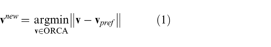
Our implementation of RVO is based on the publicly available RVO2-Library (http://gamma.cs.unc.edu/RVO2). This library implements an efficient variation of RVO that uses a set of linear constraints on an agent’s velocities, known as optimal reciprocal collision avoidance (ORCA) constraints, in order to ensure that agents avoid collisions (Van den Berg et al., 2011). Each agent is assumed to have a position, a velocity, and a preferred velocity; if an agent’s preferred velocity v _pref is forbidden by the ORCA constraints, that agent chooses the closest velocity which is not forbidden. Formally,

v^{new} = \underset{v \in ORCA}{argmin} ‖ v - v_{pref} ‖

(1)

This process is illustrated in Figure 1(a).

Fig. 1.

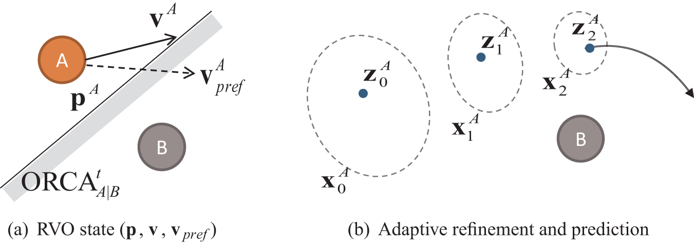
(a) RVO simulation overview: agent A’s position (p), preferred velocity (v _pref), and actual velocity (v), along with a neighboring agent B (both represented as circles). If the ORCA collision-avoidance constraints prevent an agent A from taking its preferred velocity, as shown here, the actual velocity will be the closest allowable velocity. Taken together, these elements form an agent’s RVO state x. (b) Agent state estimation: as new data is observed (blue dot) BRVO refines its estimate of a distribution of likely values of the RVO states (dashed ellipse). These parameters are then used with RVO to predict likely paths (as indicated by arrow).

An agent’s position is updated by integration over the new velocity v ^new computed in equation (1). An agent’s preferred velocity is assumed to change slowly, and is modeled by a small amount of noise during each time step. More details of the mathematical formulation are given in Section 4. A thorough derivation of ORCA constraints is given in Van den Berg et al. (2011).

BRVO uses RVO combined with a filtering process. It can replace the entire framework of offline prediction methods: LTA or ATTR, for example, and the subsequent machine learning or pre-processing of data that they require. RVO was chosen as our motion model because it is especially suitable for sensor-based applications. For example, as a velocity-based method, BRVO can handle a wide range of sampling rates and crowd densities. Force-based multi-agent simulation methods, like LTA and ATTR, compute energy potentials from the proximity of pedestrians and use these potentials as steering forces for their agents. These force-based methods thus require careful parameter tuning and small time steps to remain stable, and even with small simulation time steps, force-based methods are prone to generating oscillatory motion (Curtis et al., 2011; Köster et al., 2013). These force-based methods are thus especially problematic when using video data, which has a sensing frequency (or frame rate) of 25–30 fps, or 0.033 to 0.04 s per frame; this high sampling rate must be reduced to decrease the computational burden for interactive applications, and force-based methods are unable to cope with the larger time steps created by reducing the sample rate. Velocity-based methods, however, remain stable even when sampling rates are decreased and relatively big time steps are used. RVO, which is a velocity-based method, is shown to be stable in large time steps, as well as when simulating large, dense crowds (Curtis et al., 2012).

While we chose RVO for its stability in large time steps and dense scenarios, the motion model part of BRVO is not specific to RVO. In other words, the motion computation formulation of LTA, ATTR, or any other agent-based motion model that uses preferred velocity or short-term destination information can be used instead of RVO. Our main goal is to demonstrate how an online filtering process can be combined with an RVO-based motion model to accurately predict pedestrian trajectories.

4. BRVO

In this section, we provide the mathematical formulation of our BRVO motion model. This model combines an EnKF approach with the EM algorithm to best estimate the approximate state of each agent, as well as the uncertainty in the model.

4.1. Problem definition

In this section, we introduce our notation and the terminology used in the rest of the paper.

A pedestrian is assumed to be a human entity that shares the environment with a mobile robot. We treat pedestrians as autonomous entities that seek to avoid collisions with each other (but not necessarily with the robot). We use n to denote the number of pedestrians in the environment. We assume that a robot’s sensor produces a (noisy) estimate of the position of each pedestrian. Lastly, we assume that the robot has an estimate of impassable obstacles in the environment, represented as a series of connected line segments.

We define the computation of the BRVO motion model as a state-estimation problem. Formally, the problem we seek to solve is as follows. Given a set of observations, denoted as z ₀…z _k, for each pedestrian at time step k, we solve for the RVO state x _k that best reproduces the motion seen so far. Given this estimate, we can then use the RVO simulation model to determine the likely future path of each pedestrian.

We propose an iterative solution to this problem based on the EM algorithm. Assume that a robot is operating under a sense–plan–act loop: the robot first measures new (noisy) positions of each pedestrian, then iteratively updates its estimate of each person’s state. To do this, we run EnKF individually for each pedestrian. The joint state can be estimated using an RVO motion model. This model uses for its input the latest estimated positions of every pedestrian in the scene, and uses that input to compute the local collision avoidance of each pedestrian. Based on the prediction, the robot can create a local collision-free navigation plan for each pedestrian.

4.2. Model overview

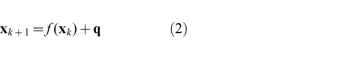
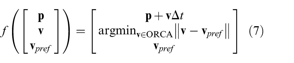
We use the RVO algorithm to represent the state of each sensed pedestrian in a robot’s environment. The state of the pedestrian at time step k is represented as a 6D vector x _k, which consists of an agent’s 2D position, 2D velocity, and 2D preferred velocity. It is important to note that the preferred velocity is included as a part of the state vector and does not need to be manually pre-determined in a scene-specific fashion. We use a Bayesian inference process to adaptively find the state that best represents all previously observed motion data (accounting for sensing uncertainty) for each pedestrian in the robot’s environment. In our case, we assume that the robot has an ability to observe the relative position of the pedestrians.

Given an agent’s RVO state x _k, we use the RVO collision-avoidance motion model, denoted here as f, to predict the agent’s next state x _k+1. We denote the state prediction error of f at each time step as q. This leads to our motion model of

x_{k + 1} = f (x_{k}) + q

(2)

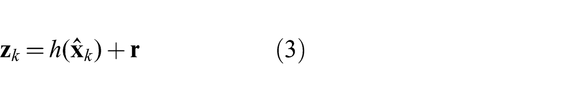
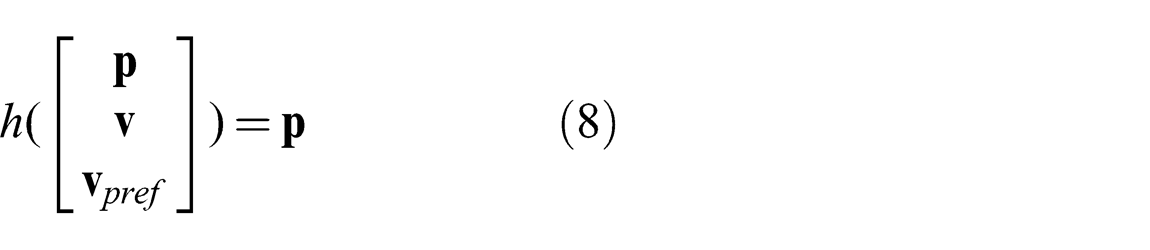
Additionally, we assume that the sensing of the robot can be represented by a function h that provides an observed state z _k, which is a function of the person’s true state ${\hat{x}}_{k}$ plus some noise from the sensing processing, which is denoted as r. That is,

z_{k} = h ({\hat{x}}_{k}) + r

(3)

An overview of this adaptive motion prediction model is given in Figure 2.

Fig. 2.

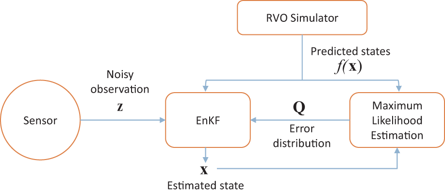
Overview of the adaptive motion model. We estimate current state x via an iterative process. Given noisy data observed by the sensor, RVO as a motion model, and the error distribution matrix Q, we estimate the current state. The error distribution matrix Q is recomputed based on the difference between the observed state and the prediction f(x), and is used to refine the current estimation of x.

Simplifying assumptions. The model given by equations (2) and (3) is very general. In order to efficiently estimate the state x _k from the observations z _k, we must make some simplifying assumptions, which allow us to develop a suitable learning approach for our adaptive model. First we assume that the error terms q and r are independent at each time step, and that they follow a zero-mean Gaussian distribution with covariances Q and R, respectively. That is,

q ~ N (0, Q)

(4)

r ~ N (0, R)

(5)

We further assume that the sensor error r is known or can be well-estimated. This is typically possible by making repeated measurements of known data points to compute the average error. In many cases, this error will be provided by the manufacturer of the sensing device. When using a tracking or recognition system to process the position input, R should be estimated from the tracking and recognition error.

To summarize, the function h is specified by the robot’s sensors, and the matrix R characterizes the estimated accuracy of these sensors. The f function is the motion model that will be used to predict the motion of each agent (here RVO), and Q represents the accuracy of this model.

Our BRVO formulation uses the RVO-based simulation model to represent the function f and EnKF to estimate the simulation parameters that best fit the observed data. At a high level, EnKF operates by representing the potential state of an agent at each time step as an ensemble (or collection) of discrete samples. Each sample is updated according to the motion model f. A mean and standard deviation of the samples is computed at every time step in order to estimate the new state.

In addition, we adapt the EM algorithm to estimate the model error Q for each agent. Better estimation of Q improves the KF process, which in turn improves the predictions given by BRVO. This process is used iteratively to predict the next state and to refine the state estimation for each agent, as depicted in Figure 1(b). More specifically, we perform the EnKF and EM steps for each agent separately while simultaneously taking into account all agents present in the motion model f(x). This gives more flexibility in dynamic scenes, allowing the method to handle cases when the robot moves or when pedestrians arrive or depart and change the number of agents in the sensed area. Because each inference step is performed per-agent on a fixed-size state (as opposed to a varying size state vector which considers all agents together), agents entering or leaving can be easily incorporated.

4.3. State representation

The above representation can be more formally summarized with the following notation. We represent each agent’s state, x, as the 6D set of RVO parameters (see Section 3.2)

x = [\begin{matrix} p \\ v \\ v_{pref} \end{matrix}]

(6)

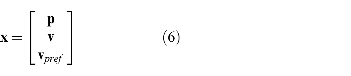
where p is the agent’s position, v the velocity, and v _pref the preferred velocity. The crowd dynamics model f is then

f ([\begin{matrix} p \\ v \\ v_{pref} \end{matrix}]) = [\begin{matrix} p + v Δ t \\ {argmin}_{v \in ORCA} ‖ v - v_{pref} ‖ \\ v_{pref} \end{matrix}]

(7)

Also, the robot can observe the relative positions of the pedestrians, which can be represented as a function h of the form

h ([\begin{matrix} p \\ v \\ v_{pref} \end{matrix}]) = p

(8)

EnKF uses some assumptions for the observation model. In general though, our BRVO framework makes no assumption about the linearity of the sensing model. More complex sensing functions (for example, advanced computer vision techniques or the integration of multiple sensors) can be represented by modifying the function h in accordance with the desired sensing model.

4.4. State estimation

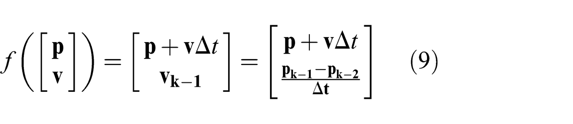
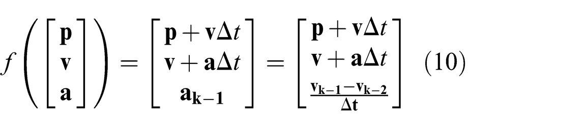
When f and h are linear functions, optimal estimation of the simulation state x _k is possible using KF. However, because f corresponds to the RVO simulation model and we can use any arbitrary sensing model h, the resulting system is a non-linear system and there is no simple way to compute the optimal estimate.

Therefore, we use EnKF, a sampling-based extension of KF, to estimate the corresponding agent state for each pedestrian. EnKF is a Bayesian filtering process, which takes as input an estimate of the prediction error $Q$ and observations z ₀…z _k and produces an estimate of the true pedestrian states x _k as a distribution of likely states $X_{k}$ . Given n pedestrians to track, each with a d-dimensional state vector, the distributions $X_{k}$ are represented in an ensemble representation where each distribution is represented by m samples. EnKF provides an estimate of the true distribution of likely pedestrian states by representing it with these m samples.

One benefit of performing EnKF for each pedestrian is that we can easily handle entering and leaving pedestrians, unlike a joint-state estimation. Instead, crowd interactions such as collision avoidance behavior is estimated by our motion model f, using the latest estimation of the pedestrians in the scene.

The ensemble representation for distributions is similar to a particle representation used in particle filters (Arulampalam et al., 2002), with the distinction that the underlying distribution is assumed to be Gaussian. The ensemble representation is widely used for estimation of systems with very large dimensional state spaces, such as climate forecasting (Hargreaves et al., 2004) and traffic conditions (Work et al., 2008). In general, the EnKF algorithm works particularly well for high-dimensional state spaces (Evensen, 2003) and can overcome some of the issues presented by non-linear dynamics (Blandin et al., 2012). For a more detailed explanation of EnKF, we refer readers to a standard textbook in statistical inference such as Casella and Berger (2002).

The motivation for this algorithmic choice is twofold. First, EnKF makes the same assumptions we laid forth in Section 4.2: that is, a (potentially) non-linear f and h combined with a Gaussian representation of error. Second, as compared to methods such as particle filters, EnKF is very computationally efficient, providing higher accuracy for a given number of samples. This is an important consideration for the low-to-medium-power onboard computers commonly found on a mobile robot, especially given a goal of online, real-time estimation.

4.5. Maximum likelihood estimation

The accuracy of the states estimated by the EnKF algorithm is a function of the parameters defined in equations (2) to (5): f, Q, h, and R. Three of these parameters are pre-determined given the problem setup: the sensing function h and the error distribution R are determined by the sensor’s specifications, and f is determined by the motion model chosen. However, the choice of motion prediction error distribution Q is still a free parameter. We propose a method of estimating the optimal value for Q based on the EM algorithm.

The EM algorithm is a generic framework for learning (locally) optimal parameters iteratively with latent variables. The algorithm alternates between two steps: an E-step, which computes expected values for various parameters, and an M-step, which computes the distribution maximizing the likelihood of the values computed during the E-step (for a more thorough discussion see McLachlan and Krishnan, 2008).

In our case, the E-step is performed via the EnKF algorithm. This step estimates the most likely state given the parameter Q. For the M-step, we need to compute Q that maximizes the likelihood of values estimated from EnKF. This probability will be maximized with the Q that best matches the observed error between the predicted state and the estimated state. We can compute this value simply by finding the average error for each sample in the ensemble at each time step for each agent.

By iteratively performing the E- and M-steps, we continuously improve our estimate of Q, which will in turn improve the quality of the learning and the predictiveness of the method. Ideally, one should iterate over the E- and M-steps until the approach converges. In practice, the process converges fairly rapidly. Due to the online process nature of our approach, we limit the number of iterations to three, which we found to be empirically sufficient. We analyze the resulting improvement produced by the EM algorithm in Section 5.1.3.

4.6. Implementation

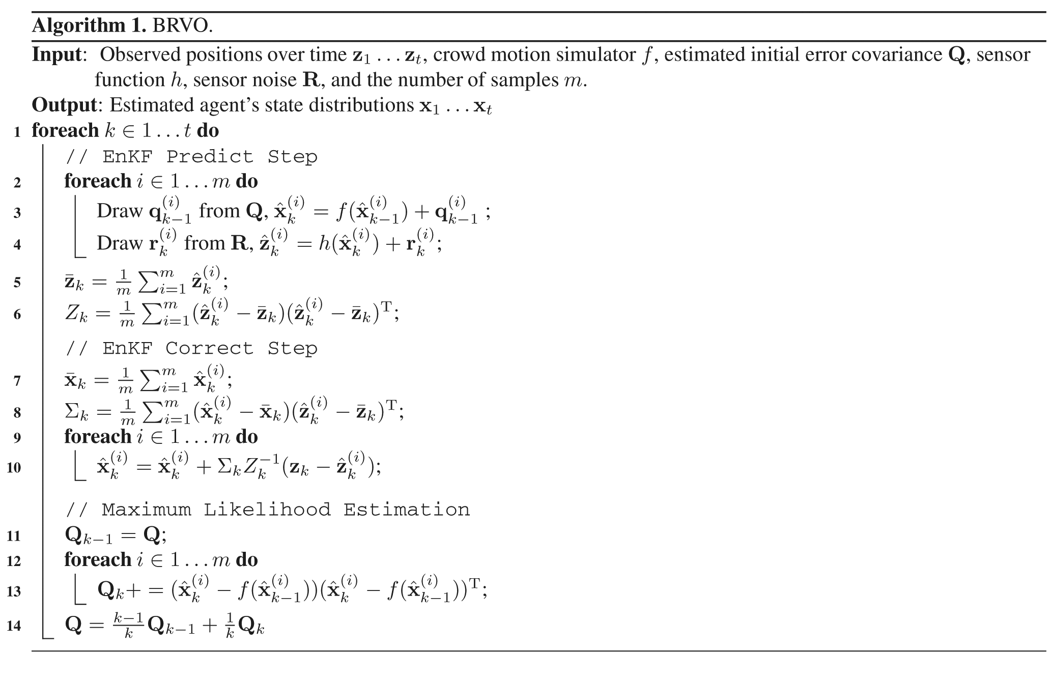
Pseudocode for our BRVO algorithm is given in Algorithm 1. We represent the distribution of likely RVO states as an ensemble of m samples. We set m = 1000 for the results shown in Section 5. Lines 2 through 6 perform a stochastic prediction of the likely next states. Lines 7 through 10 correct this predicted value based on the observed data from the robot’s sensor. Z_k is a measurement error covariance matrix, and $Σ_{k} Z_{k}^{- 1}$ is an ensemble version of the Kalman gain matrix. Lines 11 through 14 perform a maximum likelihood estimation of the uncertainty in the prediction.

Algorithm 1. BRVO.
Input: Observed positions over time z ₁…z _t, crowd motion simulator f, estimated initial error covariance Q, sensor function h, sensor noise R, and the number of samples m.
Output: Estimated agent’s state distributions x ₁…x _t
1 foreach 1 k∈ 1…t do
// EnKF Predict Step
2 foreach4 i∈ 1…m do
3 Draw $q_{k - 1}^{(i)}$ from Q, ${\hat{x}}_{k}^{(i)} = f ({\hat{x}}_{k - 1}^{(i)}) + q_{k - 1}^{(i)}$ ;
4 Draw $r_{k}^{(i)}$ from R, ${\hat{z}}_{k}^{(i)} = h ({\hat{x}}_{k}^{(i)}) + r_{k}^{(i)}$ ;
5 ${\bar{z}}_{k} = \frac{1}{m} \sum_{i = 1}^{m} {\hat{z}}_{k}^{(i)}$ ;
6 $Z_{k} = \frac{1}{m} \sum_{i = 1}^{m} ({\hat{z}}_{k}^{(i)} - {\bar{z}}_{k}) {({\hat{z}}_{k}^{(i)} - {\bar{z}}_{k})}^{T}$ ;
// EnKF Correct Step
7 ${\bar{x}}_{k} = \frac{1}{m} \sum_{i = 1}^{m} {\hat{x}}_{k}^{(i)}$ ;
8 $Σ_{k} = \frac{1}{m} \sum_{i = 1}^{m} ({\hat{x}}_{k}^{(i)} - {\bar{x}}_{k}) {({\hat{z}}_{k}^{(i)} - {\bar{z}}_{k})}^{T}$ ;
9 foreach i∈ 1…m do
10 ${\hat{x}}_{k}^{(i)} = {\hat{x}}_{k}^{(i)} + Σ_{k} Z_{k}^{- 1} (z_{k} - {\hat{z}}_{k}^{(i)})$ ;
// Maximum Likelihood Estimation
11 Q _k−1 = Q;
12 foreach i∈ 1…m do
13 $Q_{k} + = ({\hat{x}}_{k}^{(i)} - f ({\hat{x}}_{k - 1}^{(i)})) {({\hat{x}}_{k}^{(i)} - f ({\hat{x}}_{k - 1}^{(i)}))}^{T}$ ;
14 $Q = \frac{k - 1}{k} Q_{k - 1} + \frac{1}{k} Q_{k}$

5. Results and analysis

In this section, we show the results from our BRVO approach when applied to real-world datasets. We begin by isolating the effect of each component of BRVO separately, namely: EnKF, EM, and individual parameter learning (Section 5.1). We then measure the robustness of our approach across a variety of factors commonly found in real-world situations including sensor noise, low sampling rates, and spatially varying densities. Finally, we provide a quantitative comparison to other recent techniques across a variety of datasets.

Our analysis here is performed on four different datasets with various levels of noise and different sampling rates, illustrated in Figure 3. We briefly describe each dataset below.

Fig. 3.

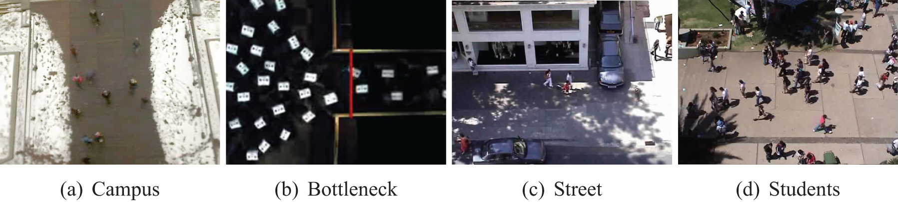
Benchmarks used for our experiments. (a) In the Campus dataset, students walk past a fixed camera in uncrowded conditions. (b) In the Bottleneck dataset, multiple cameras track participants walking into a narrow hallway. (c) In the Street dataset, a fixed camera tracks pedestrian motion on a street. (d) In the Students dataset, a fixed camera tracks students’ motion in a university.

Campus. Video data of students on campus recorded from the top of the ETH main building in Zurich, extracted manually every 0.4 s (Pellegrini et al., 2009). We extracted three sequences from this data, each containing about 10 s of pedestrian interaction: Campus-1 (7 pedestrians), Campus-2 (11 pedestrians), Campus-3 (18 pedestrians).

Bottleneck. Optical tracking equipment captured the motion of participants in a lab environment (Boltes et al., 2010). Participants moved through a bottleneck opening into a narrow passage. Data was collected with a passage width of 2.5 m. The study has about 170 participants, and we use the trajectory data subsampled at a rate of 0.4 s.

Street. This video of low-density pedestrian traffic was recorded from a street view (Lerner et al., 2009). Manually extracted pedestrian trajectories are provided with the video. The dataset contains two sequences. Street-1 contains the motion of 148 pedestrians over a period of roughly 5 min, and Street-2 contains the motion of 204 pedestrians over a period of roughly 7 min.

Students. This video was recorded from a street view (Lerner et al., 2009). The dataset contains the motion of 434 students over a period of roughly 3 min, tracked manually.

To explore the relative performance of our method we will compare it to other typical prediction approaches commonly found in robotics applications as described below.

Constant velocity (ConstVel). This model assumes that all agents will continue their most recent instantaneous velocity (inferred from the last two positions) for the immediate future (equation (9)):

f ([\begin{matrix} p \\ v \end{matrix}]) = [\begin{matrix} p + v Δ t \\ v_{k - 1} \end{matrix}] = [\begin{matrix} p + v Δ t \\ \frac{p_{k - 1} - p_{k - 2}}{Δ t} \end{matrix}]

(9)

Constant acceleration (ConstAcc). This model assumes that all agents will continue their most recent acceleration (inferred from the last two velocities) for the immediate future (equation (10)):

f ([\begin{matrix} p \\ v \\ a \end{matrix}]) = [\begin{matrix} p + v Δ t \\ v + a Δ t \\ a_{k - 1} \end{matrix}] = [\begin{matrix} p + v Δ t \\ v + a Δ t \\ \frac{v_{k - 1} - v_{k - 2}}{Δ t} \end{matrix}]

(10)

KF. We use a position- and velocity-based KF (i.e. using equation (9) as the model) which uses standard Gaussian filtering techniques to account for potential noise in the environment.

Unlike the ConstVel and ConstAcc models, using a KF will account for noise in the sensing and motion models. However, this comes at the cost of a delayed response to changes in the environment (due to data smoothing) leading to KF performing worse than ConstVel in situations where there is little noise and smooth, consistent motion. BRVO avoids this issue as demonstrated in Section 5.2.

We also compare the results against two recently proposed offline pedestrian tracking methods: LTA (Pellegrini et al., 2009) and ATTR (Yamaguchi et al., 2011). Both methods use offline training to learn models of typical pedestrian goals and speeds for a given observation area. Because of this training step, both methods are inappropriate for use in a mobile robot. However, they provide a good understanding of the state of the art in pedestrian tracking. Surprisingly, in all of the above datasets, BRVO outperforms even these offline models suggesting the flexibility of learning a model per agent outweighs the advantages from offline training. More discussion of this comparison is given in Section 5.3.

In all cases, we report errors as the distance between ground-truth (manually annotated) positions and the estimated positions. We also provide various quantitative and qualitative performance measures including the long-term prediction success rate, shapes of the trajectories, and prediction error distributions.

5.1. Method analysis

BRVO has three main components: a probabilistic Bayesian inference framework, per-agent online state estimation, and a continuing refinement of filtering parameters through the EM algorithm. Each of these components provides a substantial contribution to the overall performance.

5.1.1. EnKF for online learning

Different approaches to Bayesian inference can be used to perform the online learning task. Here we compare EnKF, particle filter, and unscented KF (Wan and Van der Merwe, 2000), all using RVO as the motion model, all without EM. For this experiment, we use the three sequences from various points in the Campus dataset.

The first five frames of ground-truth positions are used as sensor input z, and each method is issued to perform predictions for the remaining frames with the learned parameters. We use a fixed Q for each learning and prediction step: [0.5m] *I. The number of samples for both EnKF and particle filter is 50,000. We measured the mean error (squared distance) between the predicted position and ground-truth position. The results are summarized in Table 1.

Table 1.

Comparisons of different Bayesian learning algorithms. Root mean squared error between the predicted position and ground-truth position in meters (best shown in bold).

	Campus-1	Campus-2	Campus-3
EnKF	0.359	0.462	0.388
Particle filter	0.366	0.462	0.389
Unscented KF	0.476	0.501	0.420

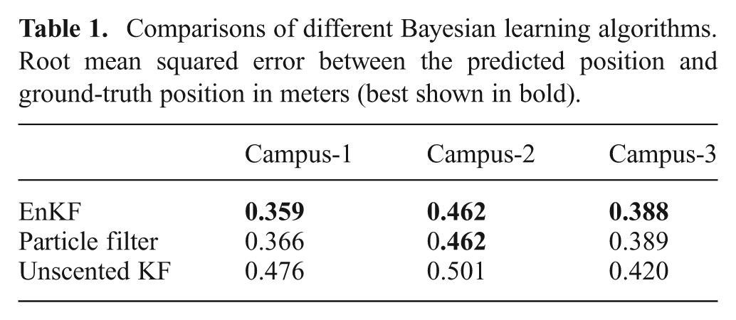
Both EnKF and particle filter outperform unscented KF, with EnKF having the best average performance. While other sampling-based approaches such as particle filters may provide similar results, EnKF’s consistent performance across these and other datasets motivated our choice of EnKF for Bayesian inference throughout this work.

5.1.2. Online vs offline learning

We can measure the improvements made by introducing the online parameter-estimation technique by comparing our method to a closely related offline approach. Following the approach proposed in LTA (Pellegrini et al., 2009) and ATTR (Yamaguchi et al., 2011), we developed an offline prediction technique based on RVO referred to here as ‘RVO-offline’. At a high level, RVO-offline uses a genetic algorithm to optimize RVO parameters to best match the training dataset of the ground-truth motion of individuals in the environment. The destination of each agent is set on the side of the environment opposite where the agent entered (as done in Pellegrini et al., 2009). For ConstVel, ConstAcc, and BRVO, we assume that we get good sensor inputs for the first two frames and compute the initial velocity for each pedestrian from the first two ground-truth positions. For RVO-offline, we assume that we have good global information about destinations and motion parameters including preferred speed, and compute the initial velocity from these parameters. We compare this RVO-offline model with the ConstVel model, the ConstAcc model, and with BRVO using the above-mentioned sequences from the Campus dataset. To compute the error, we use the first half of the dataset for training and the second half for testing. Each method attempts to predict the final agent position from the position at the halfway point. Figure 4 shows the mean error for different approaches.

Fig. 4.

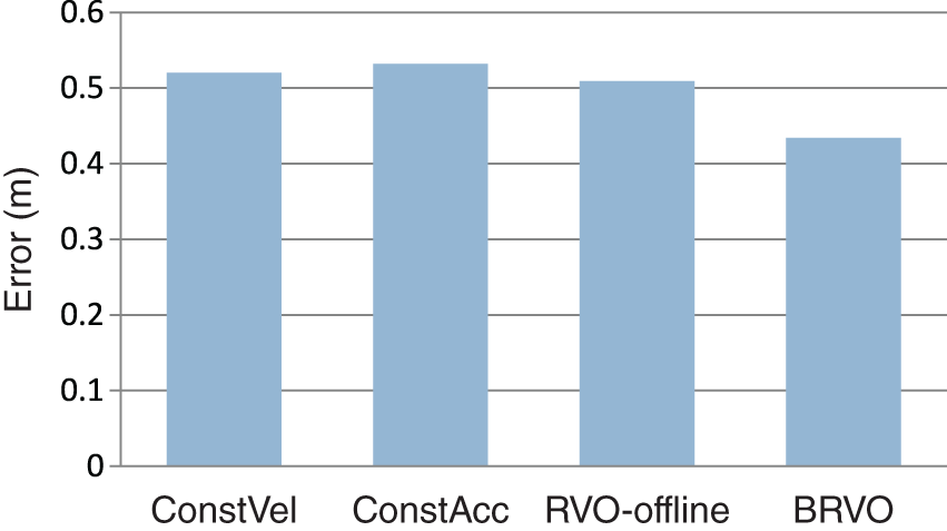
Comparison of error on Campus dataset. BRVO produces less error than ConstVel and ConstAcc predictions. Additionally, BRVO results in less error than using a static version of RVO whose parameters were fitted to the data using an offline global optimization.

While the static, offline-learning RVO model performs slightly better than the simpler motion models, BRVO offers an even more significant reduction in error, demonstrating the advantage of learning individual time-varying parameters for each agent. Additionally, unlike offline models, BRVO does not need prior knowledge of the current environment (such as likely goals), instead learning each agent’s destination dynamically through EnKF with RVO. The difficulty in choosing an individual’s goal position is one of the main challenges in using offline methods in an autonomous robot system. More discussion of the impact of goals in offline methods is given in Section 5.3.

5.1.3. EM-based estimation refinement

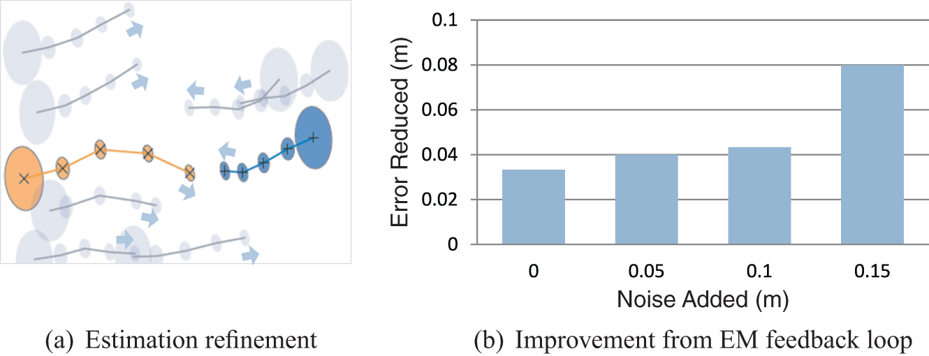
As discussed in Section 4.5, our proposed BRVO approach uses the EM algorithm to automatically refine the parameters used in the online Bayesian estimation. The effect of EM can be demonstrated visually by graphing the estimated uncertainty in the state as shown in Figure 5(a); as new data is presented and the pedestrians interact with each other, the estimated uncertainty, Q, decreases. Without the EM step, the initially given estimated uncertainty Q must be used without refining its values.

Fig. 5.

The effect of the EM algorithm. (a) The trajectory of each agent and the estimated error distribution (ellipse) for the first five frames of Campus-3 data. The estimated error distribution gradually reduces as agents interact. For two highlighted agents (orange and blue), their estimated positions are marked with ‘X’. (b) The improvement provided by the EM feedback loop for various amounts of noise. As the noise increases, this feedback becomes more important.

Figure 5(b) shows the quantitative advantage of using EM, by comparing our results in the Campus sequences with EM to those without. When using high-quality data with little noise, EM shows a slight improvement in the results. If we artificially add noise to the data (while keeping all other parameters constant), the effect of the active feedback loop becomes even more important and the EM algorithm offers increasing improvements in error estimation.

5.2. Environmental variations

Many factors in a robot’s environment can impact how well a predictive tracking method such as BRVO works. For example, poor lighting conditions can reduce the efficacy of vision-based sensors increasing the noise in the sensor data. Likewise, in dense scenarios, people can tend to change their velocities frequently to avoid collisions creating increasing uncertainty in their motion. Similarly, when a robot’s energy gets low it may choose to reduce the frequency of sampling sensor data to save power. In all of these scenarios, the difficulty in predicting a pedestrian’s motion can increase significantly. Importantly, the advantage that BRVO has over simple prediction methods grows larger as scenarios grow in complexity through additional sensor noise, more dense environments, or less frequent data readings as shown in the following experiments.

5.2.1. Noisy data

To analyze how BRVO responds to noise in the data, we compare its performance across varying levels of synthetic noise added to the ground-truth data in the Campus dataset. Like before, BRVO learns for the first five frames, and uses that information to predict the position for the remaining frames.

Figure 6 compares predictions from BRVO, ConstVel, and ConstAcc for one pedestrian’s moving right to left across the campus. The figure shows the prediction given with varying amounts of noise levels added to the training data (respectively, 0.05 m noise, 0.1 m noise, and 0.15 m noise). After the training frames, we assume that no further sensor information is given and predict the paths using only the motion models. As can be seen in the figure, BRVO reduces sensitivity to this type of noise and performs better overall at predicting both the direction of the path and the absolute speed of the pedestrian.

Fig. 6.

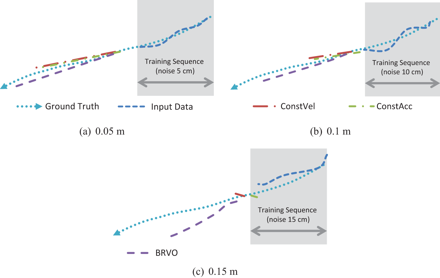
Path comparisons: the paths predicted using BRVO, ConstVel, and ConstAcc. For each case, ground-truth data with 0.05 m noise, 0.1 m noise, and 0.15 m are given as input for learning (blue dotted lines in shaded regions). BRVO produces better predictions even with a large amount of noise.

A comparison of the average prediction error across all of the Campus sequences is given in Figure 7 which compares BRVO with the ConstVel model, ConstAcc model, and KF. Both KF and BRVO are initialized with the same conditions (e.g. sensor noise and initial error covariance matrix). While adding noise always increases the prediction error, BRVO was less sensitive to the noise than other methods. Figure 8 shows the percentage of correctly predicted paths within varying accuracy thresholds. At an accuracy threshold of 0.5 m, BRVO far outperforms the ConstVel and ConstAcc models (44% vs 8% and 11% respectively) even with little noise. With larger amounts of noise, these differences tend to increase.

Fig. 7.

Mean prediction error (lower is better). Prediction error after seven frames (2.8 s) on Campus dataset. As compared to the ConstVel and ConstAcc models, BRVO can better cope with varying amounts of noise in the data.

Fig. 8.

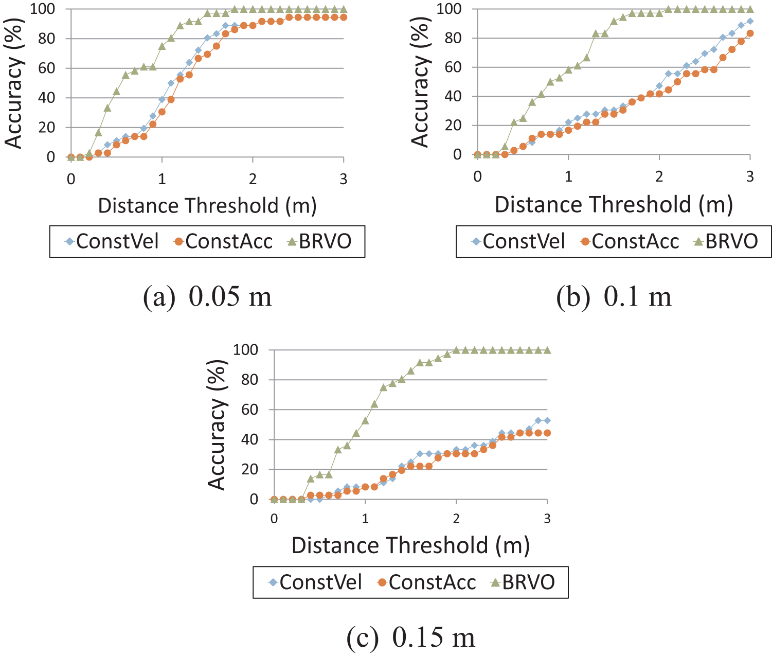
Prediction accuracy (higher is better). (a) to (c) Prediction accuracy across various accuracy thresholds. The analysis is repeated at three noise levels. For all accuracy thresholds and for all noise levels BRVO produces more accurate predictions than the ConstVel or ConstAcc models. The advantage is most significant for large amounts of noise in the sensor data, as in (c).

5.2.2. Density dependence

In a dense crowd, an individual’s motion is restricted significantly by his or her neighbors. It is thus difficult to predict pedestrian trajectories without taking into account the neighbors. Because individuals in the bottleneck scenario undergo many different densities, it provides the clearest effect of density on prediction accuracy. For analysis purposes, the scenario was spilt in three sections: a dense front section where people back-up trying to make their way through the narrow bottleneck opening (3.6 people/m²), a more moderately dense section at the entrance (3 people/m²), and the hallway itself which is less dense (2 people/m²). Note that this last region is not only the least dense, but has the simplest motion consisting primarily of moving straight through the hallway.

Figure 9 compares BRVO’s error to that of the ConstVel, ConstAcc, and KF models. The ConstVel, ConstAcc, and KF models have large variations in error for different regions of the scenario with different densities. The error is smallest in the highest density region. This is because the speed of the pedestrians is relatively slow, and the effect of the wrong prediction does not produce a large deviation from ground truth. As the density gets lower and the speed increases, we observe that the error increases. Unlike ConstVel and ConstAcc, which instantly adopt the speed, the KF model has latency adapting to the abrupt speed changes, which may have resulted in a bigger error in the lower density region. In contrast, the BRVO approach performs well across all densities because it can dynamically adapt the parameters for each agent for each frame.

Fig. 9.

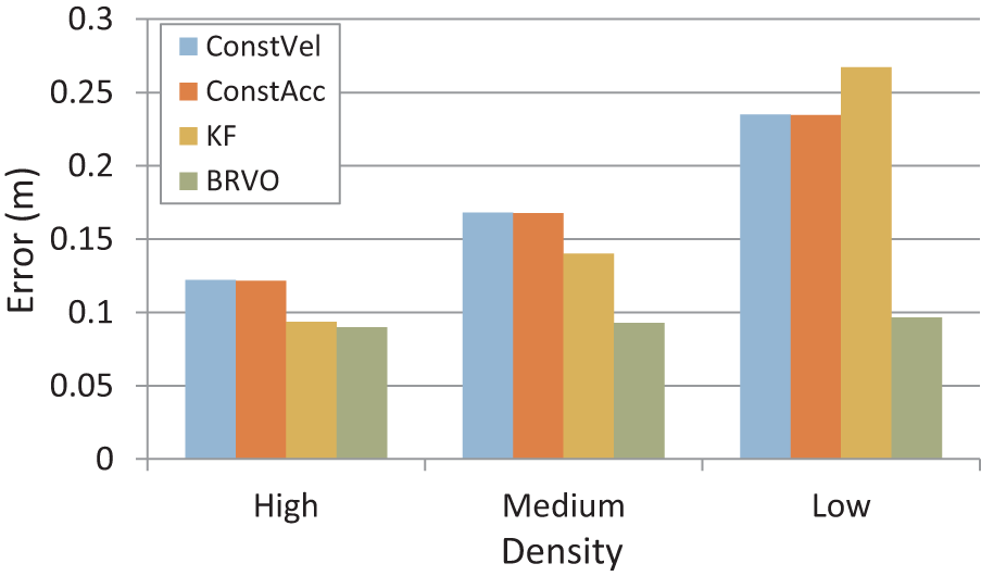
Error at various densities (lower is better). In high-density scenarios, the agents move relatively slowly, and even simple models such as ConstVel perform about as well as BRVO. However, in low- and medium-density scenarios, where the pedestrians tend to move faster, BRVO provides more accurate motion prediction than other models. KF fails to quickly adjust to rapid speed changes in the low-density region, resulting in larger errors than other methods. In general, BRVO performs consistently well across various densities.

5.2.3. Sampling rate variations

Our method also works well with very large time steps, that is, when sensor data is collected at a sparse rate over long intervals. To demonstrate this, we show the results on the Street dataset with varying sampling intervals to sub-sample the data. We chose Street-1 scenario, which has the highest frame rate (at 0.04 s per frame) of all the datasets, and then sub-sampled the data to reduce the effective frame rate. Figure 10 shows the graph of the mean error versus the sampling interval. The results show that our method performs very well compared to the ConstVel and ConstAcc models across all the sampling intervals, and has less sensitivity to low frame rates.

Fig. 10.

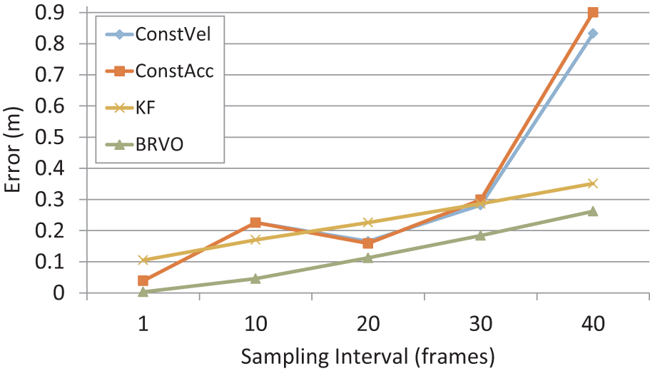
Error vs sampling interval. As the sampling interval increases, the error of ConstVel and ConstAcc estimations grows much larger than that of KF or BRVO. BRVO results have the lowest error among the four methods.

5.3. Model performance comparison

Taken together, the results provided in this section demonstrate the ability of BRVO to provide robust, high-quality motion prediction in a variety of difficult scenarios. We can directly compare our results with the results of LTA (Pellegrini et al., 2009) and ATTR (Yamaguchi et al., 2011), which report performance numbers for some of the same benchmarks. Because LTA and ATTR require offline training, we also measure the performance of KF alone in the same scenarios, in order to provide a comparison with an online method, but with a simple linear motion model.

We use the Street-1, Street-2, and Students datasets, all sampled every 1.6 s, and measure mean prediction error for every agent in the scene during the entire video sequence.

Figure 11 compares the prediction accuracy of LTA, ATTR in various configurations, KF, and BRVO with linear velocity (LIN) (the ConstVel model). Our method outperforms LTA and ATTR with an 18% to 40% error reduction rate across the three different scenarios. LTA and ATTR use the ground-truth destinations for prediction; LTA+D and ATTR+DG use destinations learned offline, as explained in Yamaguchi et al. (2011); ATTR+DG uses grouping information learned offline. Even though BRVO is an online method, it shows significant improvement in prediction accuracy on all three datasets, producing less error than other approaches.

Fig. 11.

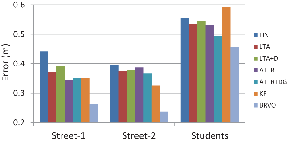
Comparison to state-of-the-art offline methods. We compare the average error of LIN, LTA, ATTR, KF, and BRVO. Our method outperforms LTA and ATTR, with an 18% to 40% error reduction rate over LIN in all three different scenarios. Significant improvement is made; compare the 4% to 16% and 7% to 20% error reduction rates of LTA and ATTR over LIN, respectively.

We observe a relatively large error when using the students dataset. This dataset is especially difficult to estimate, as explained in Yamaguchi et al. (2011); the irregular behavior of the pedestrians, including sudden stops, wandering, and chatting, reduces the predictive performance. This reduced predictability also affects the KF test, since it fails to quickly adjust to the irregular behavior.

5.4. Analysis

The ability to learn the preferred velocity on the fly comes from the BRVO framework. BRVO can be compared with other prediction methods that use motion models followed by data pre-processing and offline parameter learning (e.g. LTA or ATTR). We have shown quantitative comparisons with LTA and ATTR on three different datasets. Overall, the differences make our approach better suited to the domain of mobile robot navigation.

We can also estimate how much of BRVO’s performance improvement comes from the addition of the filtering process and how much from using the RVO motion model, although we believe that combining the motion model and filtering algorithm results in considerable improvement. To quantify the contributions of each, we provided additional comparisons: one with the constant-velocity model and one with the KF and the constant-velocity model. These two models are both online methods that use a linear motion model. The KF method is more resilient with the noisy inputs than is the ConstVel model, but adjusts more slowly when inputs change rapidly. Thus, the performance is influenced by the characteristics of the data. We have shown that our method actually outperforms both the constant-velocity and KF methods in various scenarios.

6. Robot navigation with BRVO

One potential application of our BRVO is for safer navigation for autonomous robot vehicles through areas of dense pedestrian traffic. Here we describe a simple method to integrate BRVO with the generalized velocity obstacle (GVO) motion-planning algorithm proposed in Wilkie et al. (2009) to achieve more effective navigation of a simulated car-like robot through a busy walkway. The GVO navigation method is a velocity-obstacle-based technique for navigating robots with kinematic constraints. In our case, we use car-like kinematic constraints, and we assume the robot has the ability to sense the positions of nearby moving obstacles (such as pedestrians) though with some noise. The robot uses our BRVO technique to predict the motion of each pedestrian as it navigates through the crowded walkway to its goal position.

The robot’s configuration is represented as its position (x, y) and the orientation ϕ. The robot has controls u_s and u_ϕ , which are the speed and steering angle of the robot, respectively. Figure 12 shows the kinematic model of the robot. Its constraints are defined as follows:

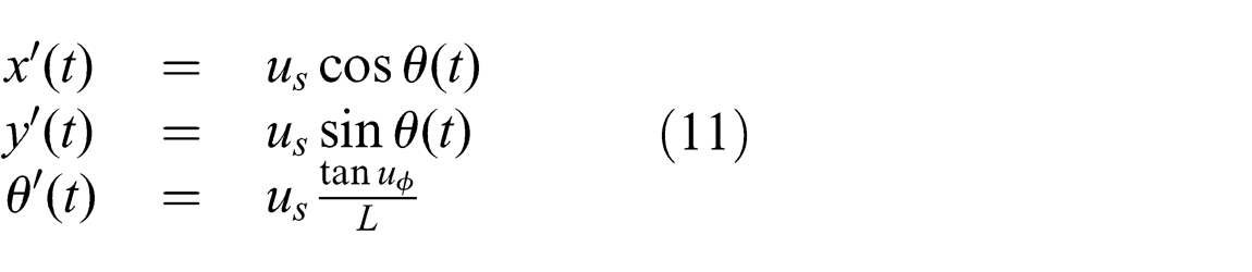
\begin{matrix} x' (t) & = & u_{s} \cos θ (t) \\ y' (t) & = & u_{s} \sin θ (t) \\ θ' (t) & = & u_{s} \frac{\tan u_{ϕ}}{L} \end{matrix}

(11)

where L is the wheelbase of the robot. We assume L = 1 m.

Fig. 12.

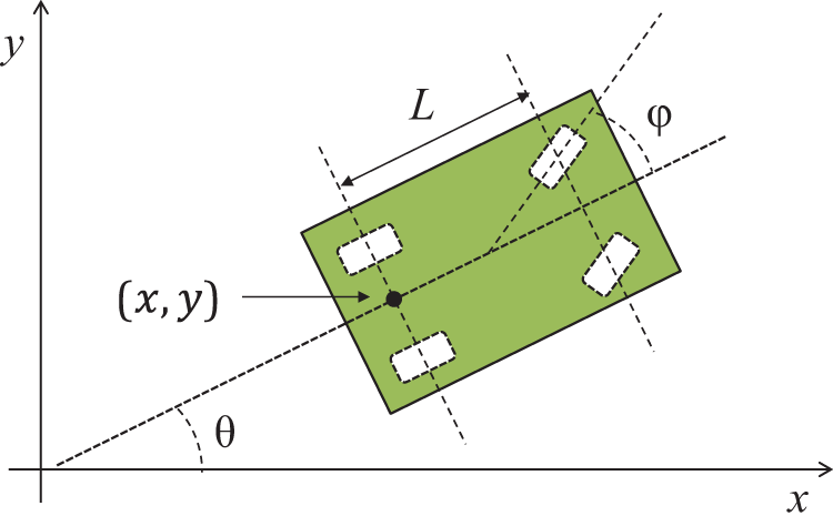
Kinematic model of the robot. The robot is modeled as a simple car at position (x, y) and with orientation θ; ɸ is a steering angle and L is a wheelbase. Our robot has the wheelbase L = 1 m.

Assuming that the control remains constant for the time interval, the robot’s position R(t, u) at time t given the control u can be derived as follows:

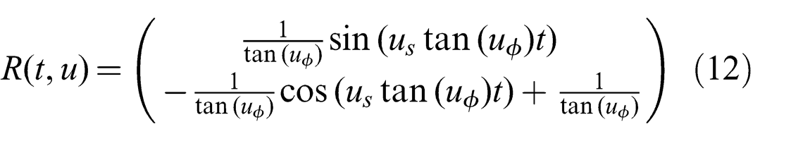
R (t, u) = (\begin{matrix} \frac{1}{\tan (u_{ϕ})} \sin (u_{s} \tan (u_{ϕ}) t) \\ - \frac{1}{\tan (u_{ϕ})} \cos (u_{s} \tan (u_{ϕ}) t) + \frac{1}{\tan (u_{ϕ})} \end{matrix})

(12)

GVO samples the space of controls for a robot to determine which controls lead to collisions with obstacles. This is done using an algebraic formulation for the minimum distance between the robot, given its kinematic model, and an obstacle, given its predicted trajectory, up to a time horizon. For our work, the minimum distance between a robot using the simple-car kinematic model and a linearly moving obstacle is derived. We limit the maximum velocity of the robot to 1.5 m/s. For each control sample, this minimum distance is solved numerically. Every control that yields a distance greater than the sum of the robot and obstacle widths is considered free. Of these free controls, a control is then selected that brings the robot closest to its goal. Formally, the actual control u is

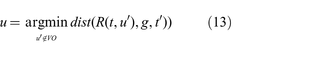
u = \underset{_{u' \notin VO}}{argmin} dist (R (t, u'), g, t'))

(13)

where u′ is subject to a velocity obstacle constraint for each moving obstacle, and VO is the velocity obstacle of the robot. Further, dist(R(t, u′), g, t′) is the minimum distance between the robot and the robot’s goal position g, over a time horizon t′. We use 5 s for t′, which is bigger than the simulation update time horizon to give a ‘look ahead’ effect. The computation of u is a slight modification from the original formulation (Wilkie et al., 2009), where u is selected from u′ which is closest to the optimal control u*. Instead of selecting the closest control, we choose the control which actually brings the robot closest to the goal.

When navigating, the robot uses BRVO to predict upcoming pedestrian motion and must avoid any steering inputs which (as determined by equation (12)) will collide with the predicted pedestrian positions. In essence, we assume a non-cooperative environment, where the pedestrians may not actively avoid collisions with the robot and the robot must assume 100% responsibility for collision avoidance (i.e. asymmetric behavior).

We use the Campus-1 (7 pedestrians), Campus-2 (11 pedestrians), and Campus-3 (18 pedestrians) data sequences from the Campus dataset to measure the performance of the robot navigation. The robot is given an initial position at one side of the walkway and is asked to move through the pedestrians to the opposite side. Given the importance of safety in pedestrian settings, if at any point the robot fails to find a collision-free trajectory which moves forward along the path, the robot will stop or turn back towards the start. Given this setup, we evaluate the percentage of times the robot is able to make it more than halfway through the pedestrian crossing without colliding with a pedestrian, or needing to stop or turn back.

We run experiments on all the three sequences, assuming a sensing error of ±15 cm noise in positional estimates, and a sampling rate of 2.5 Hz to allow adequate time for any visual processing needed to detect pedestrians in the sensed area. We collect the mean of 30 runs for each sequence; the robot’s initial position and goal position are randomly chosen for each run.

We compare the robot navigation in various combinations: GVO alone (using a constant-velocity model), GVO with GVO-KF, and GVO with BRVO. Figure 13 shows the results with GVO only (blue bars), GVO-KF (red bars), and GVO-BRVO (green bars). As the scenarios get denser, the robots navigating with GVO alone tended to avoid collisions by staying still, displaying the same freezing robot problem as discussed by other researchers (see for example Trautman and Krause, 2010). In very sparse crowds, GVO plus a linear method performs slightly better than GVO-KF, but the performance rapidly drops as the number of pedestrians increases. The GVO-BRVO algorithm improves the navigation more than GVO-KF, especially for more challenging scenarios. Compared to GVO-alone, GVO-BRVO more than doubled the task-completion rate.

Fig. 13.

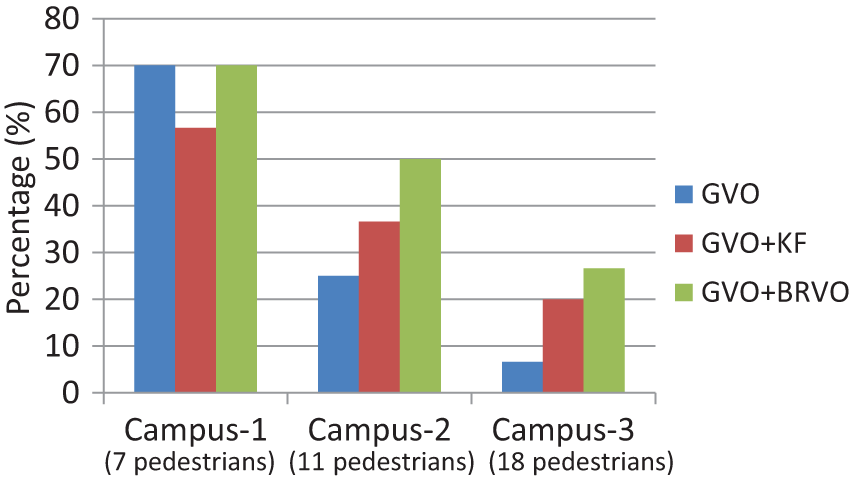
Performance of the robot navigation. We measured the percentage of the trajectories in which the robot reached farther than halfway to the goal position without any collision during the data sequence, using only GVO (blue bars), GVO-KF (red bars), and GVO-BRVO (green bars), both with 15 cm sensor noise. In many of these scenarios, using GVO for navigation often caused a robot to stop moving through the crowd to avoid collisions (the freezing robot problem). GVO-KF shows lower performance in very sparse scenarios, but outperforms the GVO-only method as the number of pedestrians increases. The GVO-BRVO algorithm further improves the navigation, especially for more challenging scenarios with more pedestrians.

Fig. 14.

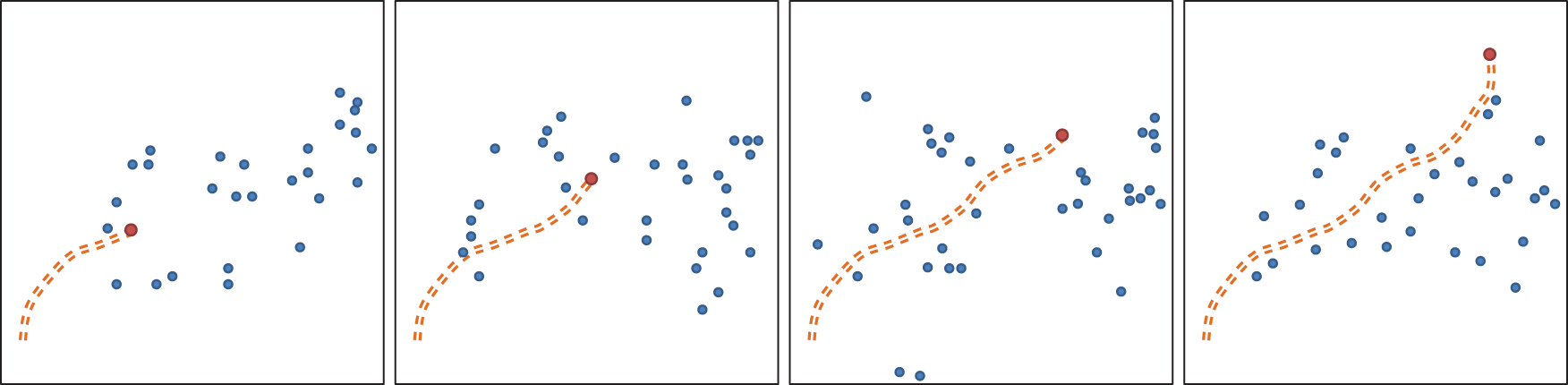
Example robot trajectory navigating through the crowd in the Students dataset. Blue circles represent current pedestrian positions, red circles are the current position of the robot, and orange dotted lines are the previous positions of the robot.

We also performed the same experiments using the ground-truth data without any sensor noise added. In this case, GVO-BRVO achieved 23% and 26% better performance over GVO-only and GVO-KF, respectively.

Similar results were seen in other datasets. Figure 3 shows an example path of the robot navigating through pedestrian motion taken from the Students dataset (with a pedestrian density of 0.35 people/m²). The result shown comes from an experimental setup with an even lower sampling rate (0.6 Hz) and using only 100 ensemble samples in EnKF. We believe that this low sampling rate, and low processing requirement, may be appropriate for many types of low-powered mobile robots. Even with these reduced computational requirements, we still achieved about a 50% task completion rate.

This series of experiments indicates that BRVO can improve planning in uncertain environments: environments with dynamic obstacles or with sensor limitations, including noisy or sparse sensor inputs. Though better prediction does not guarantee better navigation, and the freezing robot problem can still occur (Trautman and Krause, 2010), we believe that better prediction algorithms can improve the robotic navigation.

We also believe that BRVO can be combined with other robot navigation methods in a cooperative setup, since it improves the performance of RVO-based motion models in noisy-data situations, as discussed in Trautman et al. (2013). More importantly, BRVO does not need prior knowledge about the scene, such as destinations or goal positions and motion priors. BRVO-GVO, however, requires static obstacles to compute robot navigation. Motion prediction using BRVO does not require knowledge about static obstacles, although static obstacles that strongly constrain the motion of the pedestrians may improve its accuracy (e.g. Bottleneck dataset). Instead of the Bottleneck dataset, our experiments are performed without specifying the static obstacles. These features of BRVO can be a considerable benefit for navigating robots or autonomous wheelchairs in real-world scenes.

7. Conclusion and future work

We have presented a method to predict pedestrian trajectories using agent-based velocity-space reasoning. The BRVO model that we have introduced is an online motion-prediction method that learns per-agent motion models. Even without prior knowledge about the environment, it performs better than offline approaches that do have prior knowledge. We have demonstrated the benefits of our approach on several datasets, showing our model’s performance with varying amounts of sensor noise, interaction levels, and densities. Specifically, we have shown that our approach performs very well with noisy data and in low frame-rate scenarios. We also highlight BRVO’s performance in dynamic scenarios with density (spatial) and speed (temporal) variation.

BRVO assumes no prior knowledge of the scenario which it will navigate; it is thus uniquely well-suited for mobile robots that may frequently encounter new obstacles and that must handle pedestrians entering and leaving the environment. We have shown that by learning an individualized motion model for each observed pedestrian, our online motion-prediction model can perform better than less responsive offline motion models. We also showed that our method can be integrated with recent local navigation techniques to improve task completion rates and reduce instances of the freezing robot problem.

BRVO has also been used for pedestrian tracking applications and shown to increase tracking performance in various scenarios (Bera and Manocha, 2014; Liu et al., 2014). In the future, we would like to explore a method for local, dynamic group behavior estimation, to further improve the performance of BRVO.

Footnotes

Acknowledgements

We would like to thank Jur van den Berg for his help. A preliminary version of this paper appeared in .

Funding

This research is supported in part by the ARO (contract W911NF-10-1-0506), the NSF (awards 0917040, 0904990, 100057 and 1117127) and Intel.

References

Arulampalam

Maskell

Gordon

. (2002) A tutorial on particle filters for online nonlinear/non-Gaussian Bayesian tracking. IEEE Transactions on Signal Processing 50(2): 174–188.

Baker

Matthews

(2004) Lucas-Kanade 20 years on: A unifying framework. International Journal of Computer Vision 56(3): 221–255.

Bennewitz

Burgard

Cielniak

. (2005) Learning motion patterns of people for compliant robot motion. The International Journal of Robotics Research 24(1): 31–48.

Bera

Manocha

(2014) Realtime multilevel crowd tracking using reciprocal velocity obstacles. In: IEEE international conference on pattern recognition.

Blandin

Couque

Bayen

. (2012) On sequential data assimilation for scalar macroscopic traffic flow models. Physica D: Nonlinear Phenomena 241(17): 1421–1440.

Boltes

Seyfried

Steffen

. (2010) Automatic extraction of pedestrian trajectories from video recordings. In: Pedestrian and evacuation dynamics 2008, pp. 43–54.

Bruce

Gordon

(2004) Better motion prediction for people-tracking. In: Proceedings of the international conference on robotics and automation (ICRA).

Casella

Berger

(2002) Statistical Inference (Duxbury Advanced Series in Statistics and Decision Sciences). Thomson Learning: Pacific Grove. CA.

Collins

(2003) Mean-shift blob tracking through scale space. In: Proceedings of the IEEE Computer Society conference on computer vision and pattern recognition.

10.

Cui

Zha

Zhao

. (2005) Tracking multiple people using laser and vision. In: Proceedings of the IEEE/RSJ international conference on intelligent robots and systems (IROS), pp. 2116–2121.

11.

Curtis

Guy

Zafar

. (2011) Virtual Tawaf: A case study in simulating the behavior of dense, heterogeneous crowds. In: Proceedings of the IEEE international conference on computer vision workshops (ICCV workshops), pp. 128–135.

12.

Curtis

Snape

Manocha

(2012) Way portals: Efficient multi-agent navigation with line-segment goals. In: Proceedings of the ACM SIGGRAPH symposium on interactive 3D graphics and games, New York, NY, pp. 15–22.

13.

Du Toit

Burdick

(2010) Robotic motion planning in dynamic, cluttered, uncertain environments. In: Proceedings of the IEEE international conference on robotics and automation (ICRA), pp. 966–973.

14.

Evensen

(2003) The ensemble Kalman filter: Theoretical formulation. Ocean Dynamics 55: 343–367.

15.

Fod

Howard

Mataric

(2002) A laser-based people tracker. In: Proceedings of the IEEE international conference on robotics and automation (ICRA), pp. 3024–3029.

16.

Fulgenzi

Spalanzani

Laugier

(2007) Dynamic obstacle avoidance in uncertain environment combining PVOs and occupancy grid. In: Proceedings of the IEEE international conference on robotics and automation, pp. 1610–1616.

17.

Gong

Sim

Likhachev

. (2011) Multi-hypothesis motion planning for visual object tracking. In: Proceedings of the IEEE international conference on computer vision (ICCV), pp. 619–626.

18.

Guy

Chhugani

Curtis

. (2010) PLEdestrians: A least-effort approach to crowd simulation. In: Symposium on computer animation, pp. 119–128.

19.

Guy

Kim

Lin

. (2011) Simulating heterogeneous crowd behaviors using personality trait theory. In: Symposium on computer animation, pp. 43–52.

20.

Hargreaves

Annan

Edwards

. (2004) An efficient climate forecasting method using an intermediate complexity Earth System Model and the ensemble Kalman filter. Climate Dynamics 23(7): 745–760.

21.

Helbing

Molnar

(1995) Social force model for pedestrian dynamics. Physical Review E 51(5): 4282.

22.

Henry

Vollmer

Ferris

. (2010) Learning to navigate through crowded environments. In: Proceedings of the IEEE international conference on robotics and automation (ICRA), pp. 981–986.

23.

Karamouzas

Overmars

(2010) A velocity-based approach for simulating human collision avoidance. In: Albeck

Badler

Bickmore

. (eds) Intelligent Virtual Agents. New York, NY: Springer, pp. 180–186.

24.

Karamouzas

Heil

van Beek

. (2009) A predictive collision avoidance model for pedestrian simulation. In: Egges

Geraerts

Overmars

(eds) Motion in Games. Berlin: Springer, pp. 41–52.

25.

Kim

Guy

Liu

. (2012) Predicting pedestrian trajectories using velocity-space reasoning. In: The tenth international workshop on the algorithmic foundations of robotics (WAFR).

26.

Köster

Treml

Gödel

(2013) Avoiding numerical pitfalls in social force models. Physical Review E 87: 063305.

27.

Kratz

Nishino

(2011) Tracking pedestrians using local spatio-temporal motion patterns in extremely crowded scenes. IEEE Transactions on Pattern Analysis and Machine Intelligence 34(5): 987–1002.

28.

Lerner

Fitusi

Chrysanthou

. (2009) Fitting behaviors to pedestrian simulations. In: Symposium on computer animation, pp. 199–208.

29.

Liao

Fox

Hightower

. (2003) Voronoi tracking: Location estimation using sparse and noisy sensor data. In: Proceedings of the IEEE/RSJ international conference on intelligent robots and systems (IROS), pp. 723–728.

30.

Liu

Chan

Lau

RWH

. (2014) Leveraging long-term predictions and online-learning in agent-based multiple person tracking. IEEE Transactions on Circuits and System for Video Technology.

31.

Luber

Stork

Tipaldi

. (2010) People tracking with human motion predictions from social forces. In: Proceedings of the IEEE international conference on robotics and automation (ICRA), pp. 464–469.

32.

McLachlan

Krishnan

(2008) The EM Algorithm and Extensions (Wiley Series in Probability and Statistics). 2nd edn. New York, NY: Wiley-Interscience.

33.

Mehran

Oyama

Shah

(2009) Abnormal crowd behavior detection using social force model. In: Proceedings of the IEEE conference on computer vision and pattern recognition (CVPR), pp. 935–942.

34.

Pelechano

Allbeck

Badler

(2008) Virtual crowds: Methods, simulation, and control. Synthesis Lectures on Computer Graphics and Animation 3(1): 1–176.

35.

Pellegrini

Ess

Schindler

. (2009) You’ll never walk alone: Modeling social behavior for multi-target tracking. In: Proceedings of the IEEE 12th international conference on computer vision, pp. 261–268.

36.

Pettré

Ondrej

Olivier

. (2009) Experiment-based modeling, simulation and validation of interactions between virtual walkers. In: Symposium on computer animation, pp. 189–198.

37.

Pradhan

Burg

Birchfield

(2011) Robot crowd navigation using predictive position fields in the potential function framework. In: American control conference (ACC), pp. 4628–4633.

38.

Reynolds

(1999) Steering behaviors for autonomous characters. In: Game developers conference.

39.

Rodriguez

Ali

Kanade

(2009) Tracking in unstructured crowded scenes. In: Proceedings of the IEEE 12th international conference on computer vision, pp. 1389–1396.

40.

Schadschneider

Klingsch

Klüpfel

. (2009) Evacuation dynamics: Empirical results, modeling and applications. In: Meyers

(ed) Encyclopedia of Complexity and Systems Science. New York: Springer, pp. 3142–3176.

41.

Schulz

Burgard

Fox

. (2003) People tracking with mobile robots using sample-based joint probabilistic data association filters. The International Journal of Robotics Research 22(2): 99.

42.

Snape

van den Berg

Guy

. (2011) The hybrid reciprocal velocity obstacle. IEEE Transactions on Robotics (TRO) 27(4): 696–706.

43.

Svenstrup

Bak

Andersen

(2010) Trajectory planning for robots in dynamic human environments. In: Proceedings of the IEEE/RSJ international conference on intelligent robots and systems (IROS), pp. 4293–4298.

44.

Trautman

Krause

(2010) Unfreezing the robot: Navigation in dense, interacting crowds. In: Proceedings of the IEEE/RSJ international conference on intelligent robots and systems (IROS), pp. 797–803.

45.

Trautman

Murray

. (2013) Robot navigation in dense human crowds: The case for cooperation. In: Proceedings of the IEEE international conference on robotics and automation (ICRA), pp. 2153–2160.

46.

Treuille

Cooper

Popovi

(2006) Continuum crowds. In: ACM SIGGRAPH, pp. 1160–1168.

47.

Van den Berg

Guy

Lin

. (2011) Reciprocal n -body collision avoidance. In: Pradalier

Siegwart

Hirzinger

(eds) Robotics Research: The 14th International Symposium ISRR (Springer Tracts in Advanced Robotics). Berlin: Springer-Verlag, pp. 3–19.

48.

Van den Berg

Lin

Manocha

(2008a) Reciprocal velocity obstacles for real-time multi-agent navigation. In: Proceedings of the IEEE international conference on robotics and automation (ICRA), pp. 1928–1935.

49.

Van den Berg

Patil

Sewall

. (2008b) Interactive navigation of individual agents in crowded environments. In: Symposium on interactive 3D graphics and games (I3D).

50.

Wan

Van der Merwe

(2000) The unscented Kalman filter for nonlinear estimation. In: Proceedings of the IEEE adaptive systems for signal processing, communications, and control symposium, pp. 153–158.

51.

Wilkie

van den Berg

Manocha

(2009) Generalized velocity obstacles. In: Proceedings of the IEEE/RSJ international conference on intelligent robots and systems, Piscataway, NJ, pp. 5573–5578.

52.

Work

Tossavainen

Blandin

. (2008) An ensemble Kalman filtering approach to highway traffic estimation using GPS enabled mobile devices. In: 47th IEEE conference on decision and control, pp. 5062–5068.

53.

Yamaguchi

Berg

Ortiz

. (2011) Who are you with and where are you going? In: Proceedings of the IEEE conference on computer vision and pattern recognition, pp. 1345–1352.

54.

Ziebart

Ratliff

Gallagher

. (2009) Planning-based prediction for pedestrians. In: Proceedings of the IEEE/RSJ international conference on intelligent robots and systems (IROS), Piscataway, NJ, pp. 3931–3936.