Communication-aware information gathering with dynamic information flow

3.1. Dynamic information flow

Our goal is to maximize information gain by controlling the flow of information within a decentralized information gathering system subject to communication and processing constraints. Data is continuously produced by sensors and consumed by other elements of the system. We first define a graph structure that models these system elements and the data flow between elements. Given such a model, we then define the dynamic information flow problem in general form.

A decentralized information gathering system is a configuration of several elemental components. Sensors are elements that generate sensor data measured by physical sensing devices, such as laser scanners and cameras. Data from such sensors are transformed into observations by applying algorithms such as object detection and classification. Processors are computational elements that perform these processing tasks. Processors may be cascaded if necessary. The observations generated by processors act as input into estimator elements that maintain belief states. For example, an estimator could be an extended Kalman filter (EKF) in the tracking case or an occupancy grid in the mapping case.

Data flows via a communication system from sensors to processors, from processors to other processors and from processors to estimators. The topology of the resulting network is a directed acyclic graph, where information value, communication limits and computation limits induce costs or capacity constraints on the links in the graph. The induced link costs may vary according to the properties of the underlying communication mechanism, which may not be the same for all links. Elements of the system generally are physically distributed among multiple robots or ground stations and therefore communicate using an inter-robot communication system such as a wireless network. It is also possible for multiple elements to reside within a single physical platform and communicate using an intra-robot communication system such as a wired network or in-memory communication.

These system elements can also be viewed in terms of the well-known network flow problem (Ahuja et al., 1993) as follows. The commodity that flows through the network in this case is information in the form of sensor data or processed observations. Sensors correspond to supply nodes, estimators correspond to demand nodes, and processors correspond to intermediate, or transshipment, nodes. Communication links between nodes correspond to arcs or links between nodes of the network.

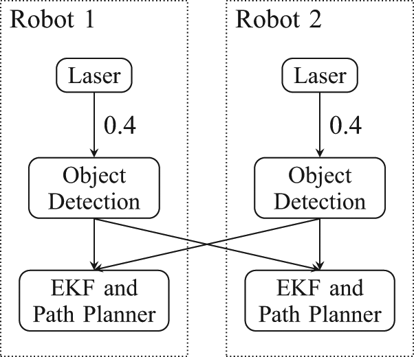
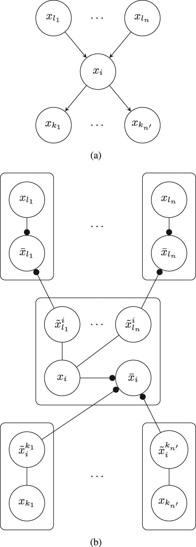
An example diagram of a decentralized information gathering system is shown in Figure 1(a) with the corresponding system topology represented by the directed acyclic graph shown in Figure 1(b). These diagrams could correspond, for example, to the case of two robots tracking a target using different types of sensors and with access to an off-board processing station. For target detection, each robot either processes its raw sensor data on-board or transmits the data to be processed off-board. Moreover, the robots can choose to either share raw sensor data or processed point observations instead.

OPEN IN VIEWER

Fig. 1.

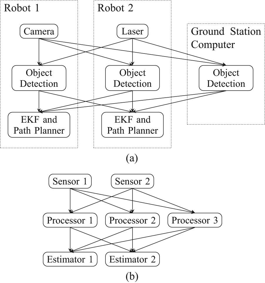
(a) An example of a decentralized information gathering system with two robots and one off-board processor. (b) The corresponding network topology in our dynamic information flow formulation.

Formally, a decentralized information gathering team is represented by a directed acyclic graph (DAG) G = {V, E} where V is the set of vertices (or equivalently, nodes) and E is the set of edges or links. In the graph G, for every i, k ∈ V, if (i, k) ∈ E then we say that k is a child node of i and i is a parent node of k. The set C ( i ) = { k ∈ V : ( i , k ) ∈ E } is the set of children of node i. Similarly, the set P ( k ) = { i ∈ V : ( i , k ) ∈ E } is defined as the set of parents of node k. We define N ( i ) = P ( i ) ∪ C ( i ) as the neighborhood of node i. A node with no parents is called a head node. A node with no children is called a tail node. We denote the depth of the graph G as κ(G) defined as the number of nodes in the longest path from a head node to a tail node. The set C ¯ ( i ) = { k ∈ V : there exists a directed path from i to k} is referred to as the set of successors of node i. The set P ¯ ( k ) = { i ∈ V : there exists a directed path from i to k} is referred to as the set of ancestors of node i.

The set of nodes is partitioned into three mutually exclusive subsets: the set of sensors V_s which act as sources, the set of processor nodes V_p which act as intermediate nodes and the set of estimator nodes V_e which act as destination nodes. Links connect nodes in V_s to nodes in V_p , nodes within V_p and nodes in V_p to nodes in V_e .

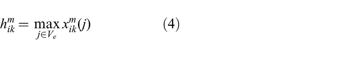
Sensor data is multicast from each sensor node m ∈ V_s to all connected estimator nodes j ∈ V_e . Sensor m produces data at a fixed rate and this data is consumed by connected estimators at the same rate. To represent this production/consumption rate we introduce the variable r i m ( j ) at node i for each sensor m and destination j. Variable r i m ( j ) is called the inward flow and is set to sensor m’s data rate if i = m or else the negative of sensor m’s data rate if i = j or 0 otherwise. The average data rate of the flow passing through link (i, k) originating from source m and destined to j is defined as x ik m ( j ) . As an example, Figure 2 shows a graph of an acyclic network with a single source. The inward flow variables are indicated for the source and destination nodes. A possible flow variable configuration is also shown for each link inside square brackets. The left entry is for j ₁ and the right entry is for j ₂.

OPEN IN VIEWER

Fig. 2.

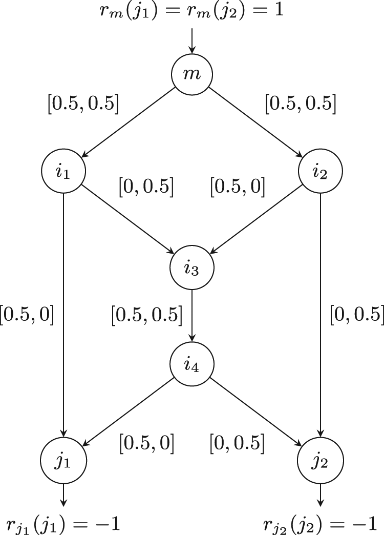
An example routing configuration for the butterfly network. Numbers within brackets are the flow values for each link. The first value corresponds to destination j ₁ and the second corresponds to destination j ₂.

A set of flow variables { x ik m ( j ) : j ∈ V e } will lead to an average total flow of h^m _ik on link (i, k). The relation between the total flow and the destination-specific flow variables will also depend on the underlying multicast implementation. With network coding, the total flow is simply the maximum flow over all destinations as defined in (1) (Ahlswede et al., 2000). This relation will be assumed for the current problem formulation. The general validity of this assumption is further discussed in Section 4.3:

h ik m = max j ∈ V e x ik m ( j )

(1)

Communication load, computation load and sensor observation utility induce a net link cost of c ik m per unit of data flow from source m passing through link (i, k). The link cost is multiplied by the total flow h ik m to obtain the total link cost arising from source m. Summing over all sources, link (i, k) has a total cost of ∑ m c ik m h ik m .

Sensor observations induce a reward when reaching an estimator. In order to represent this reward, the information value of sensor m to estimator j is subtracted from the cost of each link incident to j.

Because a sensor observation may have little value for a given estimator, the system requires a mechanism by which a sensor can decide not to send any data to a certain destination. We model this option by adding a virtual, zero-cost link directly from each sensor to all connected estimators.

We now define the general dynamic information flow problem as follows. Given link costs { c ik m } and inward flow rates { r i m ( j ) } , choose the set of flow variables { x ik m ( j ) } such that the total cost summed over all links in the network is minimized subject to constraints. Link costs and constraints may vary over time.

3.2. Min-cost-DIF

We define the first concrete form of the general problem, min-cost-DIF, according to the constrained optimization (2)–(5). Information value, communication and computation resource demand are represented using link costs. This formulation is appropriate for situations where the relative costs between the items are known a priori:

minimize ∑ ( i , k ) ∈ E , m ∈ V s c ik m h ik m

(2)

subject to x ik m ( j ) ≥ 0

(3)

h ik m = max j ∈ V e x ik m ( j )

(4)

∑ l ∈ P ( i ) x li m ( j ) − ∑ k ∈ C ( i ) x ik m ( j ) + r i m ( j ) = 0

(5)

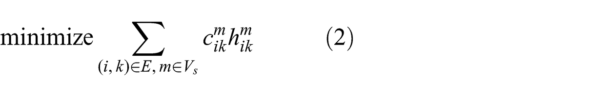
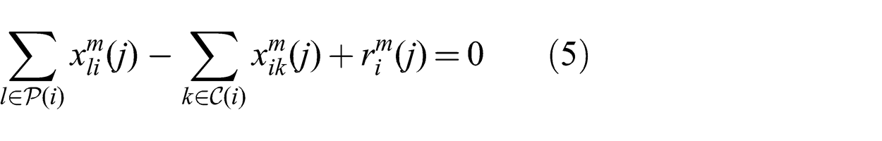
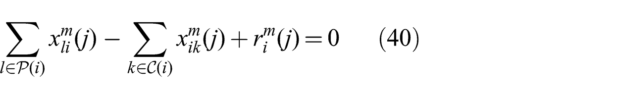
The first constraint (3) ensures that flow is always positive. The second constraint (4) represents the multicast condition and the third constraint (5) ensures that the sum of all inward and outward flow at a node is zero.

In min-cost-DIF, link costs may change over time due to changes in communication and processing costs as well as changes in sensor utility. For example, robots may move closer to or further away from each other, resulting in a change in communication costs. Sensor viewpoint may also change, leading to a change in the value of on-board sensor observations.

3.3. Threshold-DIF

We introduce a second problem variant, threshold-DIF, to represent the case where the correct scale between communication costs, computation costs and information value is not known a priori. In this case, communication bandwidth and processing power are viewed as limited resources. The goal of threshold-DIF is thus to maximize information gain subject to communication bandwidth and processing power constraints.

We augment (2) to (5) to include two additional constraints (6) and (7) and define three additional input parameters, ν ik m , C_ik and K_s , to represent resource capacity limits. Constraint (6) bounds the weighted sum of flows originating from different sensors to respect a fixed capacity C_ik . The summation over all sensors in V_s is required since a link may carry messages originating from different sensors. Weights { ν ik m } are used to scale flow values h ik m on a per-link basis. For example, variations in required communication bandwidth due to link quality can be modeled by assigning appropriate values to { ν ik m } . Similar to link costs, these variables may change over time:

∑ m ∈ V s ν ik m h ik m ≤ C ik

(6)

∑ ( i , k ) ∈ S s ∑ m ν ik m h ik m ≤ K s

(7)

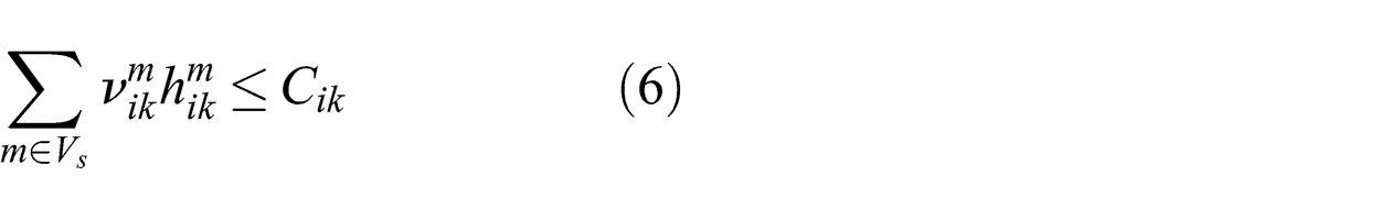
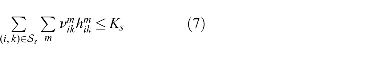
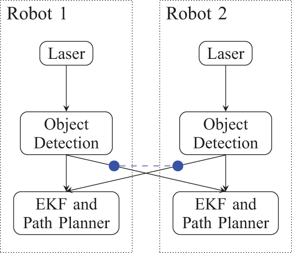
To motivate constraint (7), consider the decentralized information gathering network diagram in Figure 3 which is a subset of the diagram in Figure 1. If the two robots in this example exclusively use wireless communications to share observations, then all four links that cross the robot boundaries share a common resource (the wireless communication medium). This constraint is indicated in the figure by the dashed link. Moreover, if each robot only uses one computer for all processing requirements then the links from both sensors to each of the object detection modules share another common resource, the on-board processing computer. These constraints are indicated in the figure by dotted links. This class of constraints, which we call inter-link constraints, is represented in (7), where K_s is a fixed upper bound on resource s and S s is the set of links sharing resource s. Again, the flow rates are weighted because inter-link constraints impose bounds on the total flow across different links. These links could either be emanating from different nodes, as shown in the example in Figure 3, or from the same node, when a node sends to many nodes using the same medium.

OPEN IN VIEWER

Fig. 3.

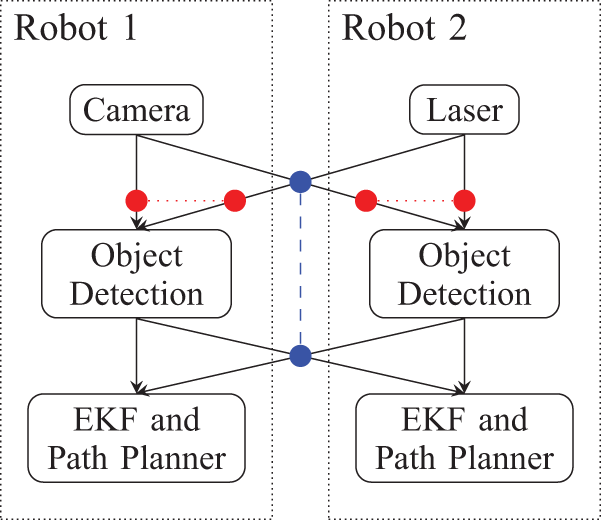
An example of a system with inter-link constraints. Links tagged with the dashed line share a wireless communication medium, while those tagged with a dotted line share a common processing resource.

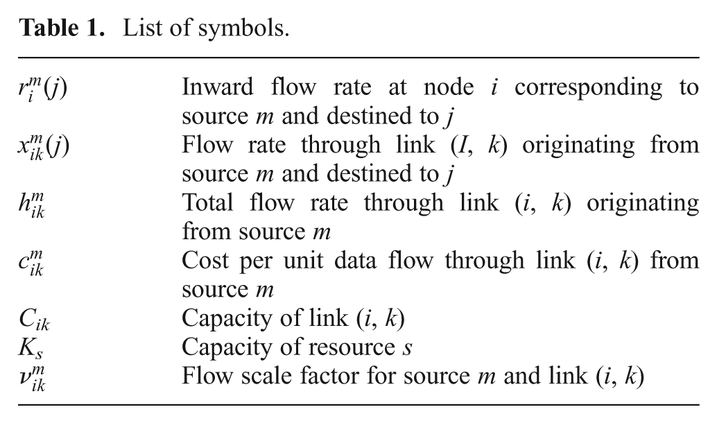
For convenience, the main terms used in the DIF problem formulation are listed in Table 1. We note that i, k, m and j all correspond to nodes in the network graph. We use m to denote a source node, j to denote a destination node, i to denote the incumbent node and k to denote the incident node of an edge.

OPEN IN VIEWER

Table 1.

List of symbols.

r i m ( j )	Inward flow rate at node i corresponding to source m and destined to j
x ik m ( j )	Flow rate through link (I, k) originating from source m and destined to j
h ik m	Total flow rate through link (i, k) originating from source m
c ik m	Cost per unit data flow through link (i, k) from source m
Cik	Capacity of link (i, k)
Ks	Capacity of resource s
ν ik m	Flow scale factor for source m and link (i, k)

3.4. Sensor utility

Sensor utility in the DIF formulation is a measure of the relative importance of sensor data with respect to a specific estimator. The importance of sensor data is evaluated based on the improvement it induces in the estimate. Hence, sensor utility depends both on the sensor and on the current state of the estimator. Sensor utility can be computed exactly using the Partially observable Markov decision process (POMDP) formulation of the information gathering problem; however, this is intractable since Dec-POMDPs are nondeterministic exponential time-complete (Bernstein et al., 2002). In Section 4.3, we present a myopic approximation to sensor utility that was used in our experiments. A further discussion of the issue of sensor utility approximation is provided in Section 7.

4.1. Min-cost-DIF using multicast network routing

An instance of min-cost-DIF can be transformed into an instance of multicast network routing (Cui et al., 2007; Xi and Yeh, 2010) as follows. The flow variable x_ik (j) is replaced with t_i (j)ϕ_ik (j), where t_i (j) is the total flow passing through i and destined to j while ϕ_ik (j) is the routing variable for link (i, k); more specifically, it is the fraction of t_i (j) that is routed to k.

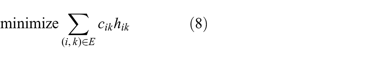
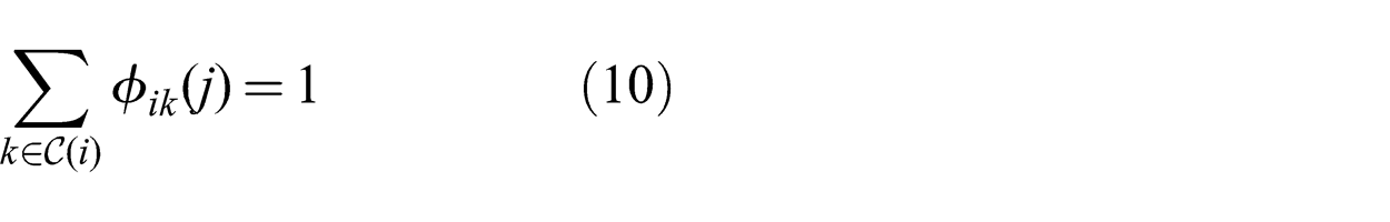
Following this change of variables, the resulting formulation is given by the optimization problem (8)–(12). Constraint (10) states that the sum of the routing variables for each node is equal to one, while (11) and (12) are equivalent to (4) and (5):

minimize ∑ ( i , k ) ∈ E c ik h ik

(8)

subject to ϕ ik ( j ) ≥ 0

(9)

∑ k ∈ C ( i ) ϕ ik ( j ) = 1

(10)

h ik = max j t i ( j ) ϕ ik ( j )

(11)

t i ( j ) = r i ( j ) + ∑ l ∈ P ( i ) t l ( j ) ϕ li ( j )

(12)

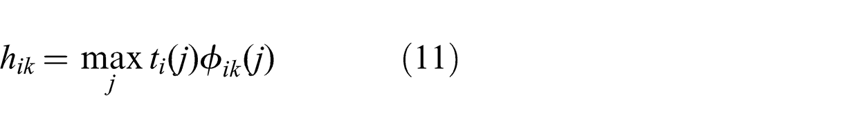
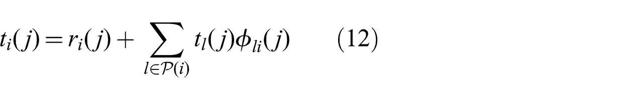
Given this mapping, existing algorithms for multicast network routing can be applied. Here we summarize one such algorithm, originally presented in Cui et al. (2007). The algorithm is based on message passing and relies on obtaining the marginal cost δ_ik (j) for each link. The marginal cost is the rate at which the total cost increases due to a unit increase in flow along that link and is given by (13):

δ i k ( j ) = { c i k / n + ∑ l ∈ C ( k ) ϕ k l ( j ) δ k l ( j ) if t i ( j ) ϕ i k ( j ) and n - 1 other flows on link ( i , k ) are the maximum ∑ l ∈ C ( k ) ϕ k l ( j ) δ k l ( j ) otherwise

(13)

Min-cost-DIF can be solved for each source m independently and in parallel. The full problem can be decomposed into independent sub-problems, one for each source, since the objective is additive and there are no inter-source constraints. This is evident from the problem formulation (2)–(5). Therefore, for simplicity of notation the subscript m is dropped from all variables in this section.

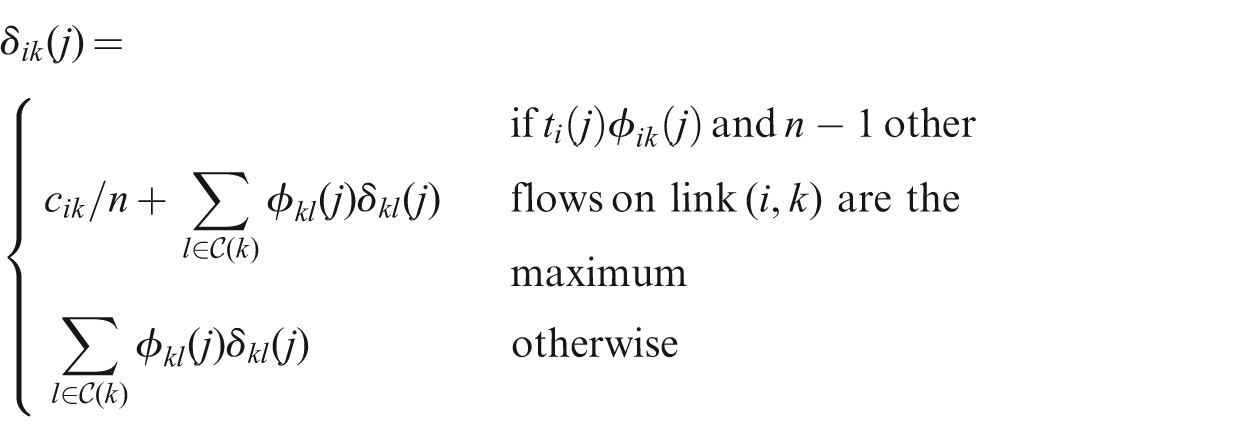
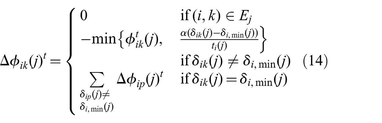
At the start of the algorithm, the routing variables {ϕ_ik (j)} are initialized arbitrarily such that they obey constraints (9) and (10). The routing variables are then repeatedly updated such that after iteration t the routing variables are set as ϕ ik t + 1 ( j ) = ϕ ik t ( j ) + Δ ϕ ik ( j ) t . The update direction Δϕ_ik (j) ^t is defined in (14) where E_j is the set of edges belonging to the subgraph containing the ancestors of destination j and δ_i, _min(j) = min _k δ_ik (j):

Δ ϕ ik ( j ) t = { 0 if ( i , k ) ∈ E j − min { ϕ ik t ( j ) , α ( δ ik ( j ) − δ i , min ( j ) ) t i ( j ) } if δ ik ( j ) ≠ δ i , min ( j ) ∑ δ ip ( j ) ≠ δ i , min ( j ) Δ ϕ ip ( j ) t if δ ik ( j ) = δ i , min ( j )

(14)

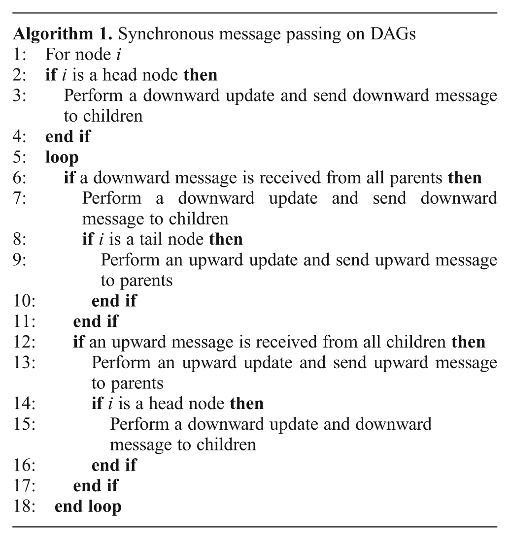
The algorithm runs synchronously. First, the head nodes send messages with their flow contributions to their children. Once a node receives messages from all of its parents, it passes the message to its own children and so forth. The purpose of this downward sweep is to allow nodes to compute the flow of the current routing configuration. The flow values are necessary to compute the marginal costs required in the upward sweep. The downward sweep is followed by an upward sweep during which the marginal costs are computed according to (13) and the routing variables are updated according to (14). The downward and upward sweeps are decentralized, synchronous and are guaranteed to visit every node. Their sequence is dictated by Algorithm 1. The synchronicity property of Algorithm 1 is proved in Lemma 1.

OPEN IN VIEWER

Algorithm 1. Synchronous message passing on DAGs
1: For node i
2: if i is a head node then
3:  Perform a downward update and send downward message to children
4: end if
5: loop
6:  if a downward message is received from all parents then
7:   Perform a downward update and send downward message to children
8:   if i is a tail node then
9:    Perform an upward update and send upward message to parents
10:   end if
11:  end if
12:  if an upward message is received from all children then
13:   Perform an upward update and send upward message to parents
14:   if i is a head node then
15:    Perform a downward update and downward message to children
16:   end if
17:  end if
18: end loop

Due to possible changes in link costs, this message passing optimization runs continuously throughout system operation. As the system configuration changes, link costs are updated with new values. To ensure convergence, the interval between updates is set to an adequate time period. Further details on the appropriate length of the interval between updates can be found in Section 4.3.

Lemma 1. In Algorithm 1, after node i has performed its t-th downward update and before forwarding this update:

Proof. Suppose one of node i’s successors has performed t′ > t − 1 upward updates. This means that at least one tail node in the successors has performed t′ downward updates. This is impossible because node i has only yet forwarded t − 1 downward messages. Since node i has performed t updates then its ancestors have performed at least t updates. Now, suppose one of node i’s ancestors has performed t″ updates where t″ > t. Then, the head nodes in the ancestry have performed at least t″ updates. This in turn means that they have performed t″ − 1 upward updates which means the tail nodes have performed t″ − 1 > t − 1 updates, which is impossible as just shown. This means that node i has forwarded at least t′ − 1 ≥ t downward updates, which leads to a contradiction.□

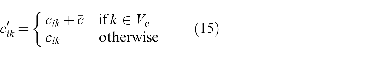
Due to observation rewards, negative costs may be assigned to links incident to an estimator j ∈ V_e . These negative costs are handled within the framework of the multicast network routing algorithm by solving an equivalent problem. A large enough constant c ¯ is added to all {c_ij : j ∈ V_e } to obtain a set of non-negative cost variables {c′ _ik } defined in (15).

The equivalence of solving the optimization problem (8)–(12) to solving the problem with cost variable c′ _ik instead of c_ik is proved in Theorem 1:

c ′ ik = { c ik + c ¯ if k ∈ V e c ik otherwise

(15)

Theorem 1. Replacing link cost c_ik in problem (8)–(12) with c′_ik defined in (15) results in a problem equivalent to (8)–(12).

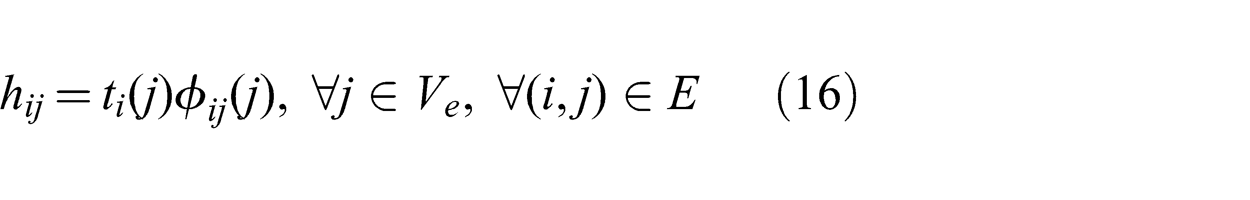
Proof. For every link (i, j) such that j ∈ V_e , constraint (11) turns into the equality relation (16) instead since the only flow that should run along that link is the flow destined to estimator j:

h ij = t i ( j ) ϕ ij ( j ) , ∀ j ∈ V e , ∀ ( i , j ) ∈ E

(16)

After adding c ¯ to the cost of these links to obtain {c′ _ij }, a total of c ¯ ∑ ( i , j ) h ij is added to the problem objective. Since c ¯ is constant, we now proceed to prove that ∑ ( i , j ) h ij is constant. After substituting h_ij from (16), we obtain (17):

∑ ( i , j ) h ij = ∑ j ∈ V e ∑ i ∈ P ( j ) t i ( j ) ϕ ij ( j )

(17)

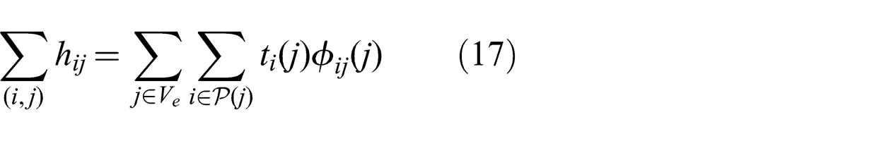
The right-hand side of the equation is equal to the total flow arriving at a destination node summed over all destinations. By definition, this flow is equal to the source flow multiplied by the number of destinations and hence is constant.

4.2. Analysis

Subject to the choice of step size parameter α, the multicast routing algorithm is guaranteed to converge to the global optimum (Cui et al., 2007). Since a DAG contains no loops by definition, no contingencies are required to avoid routing loops. By Theorem 1, a min-cost-DIF instance with negative costs on links to an estimator can still be solved using the multicast routing algorithm by adding a sufficiently large positive constant to all such links.

The running time of multicast network routing with network coding is not explicitly provided in Xi and Yeh (2010) and Cui et al. (2007) but is implied to be polynomial in the size of the network. In practice, we have observed a polynomial rate of increase as a function of network size, as shown in Section 4.3 below.

4.3. Implementation and scalability

Implementing multicast routing for min-cost-DIF involves three main challenges. First, we need to allow all nodes to find the available sources and destinations in a decentralized manner. Second, we need to ensure that the nodes have a suitable mechanism to compute any changing input parameters. Finally, we must choose a suitable multicast policy to implement the chosen flow rates {x_ik (j)}.

Each node must find the set of sources and destinations to which it is connected in the network. Initially, each node is aware of its direct neighbors only. By performing only one downward sweep and one upward sweep of message passing described in Algorithm 1, each node can obtain the list of sources and destinations to which it is connected. In our implementation, the downward messages contain the set of source identities received so far and the upward messages contain the set of destination identities received so far.

Link costs are continuously computed due to changes in the team configuration throughout the progress of its mission. In our implementation, communication costs are simply set proportional to inter-robot distance. Processing costs are assumed to be constant throughout the system operation. Sensor utility, on the other hand, can be more difficult to compute since each estimator must receive observations from a sensor in order to evaluate this utility. We maintain sensor utility values dynamically though an exploration–exploitation model. Each node obeys the chosen flow rate x_ik (j) with probability (1−ε) (exploitation) and switches to another randomly selected flow rate with probability ε (exploration). The value of ε is set to a small positive number less than one. More sophisticated alternatives using machine learning methods are possible, such as in Xu et al. (2013a). Section 7 provides further discussion on this issue.

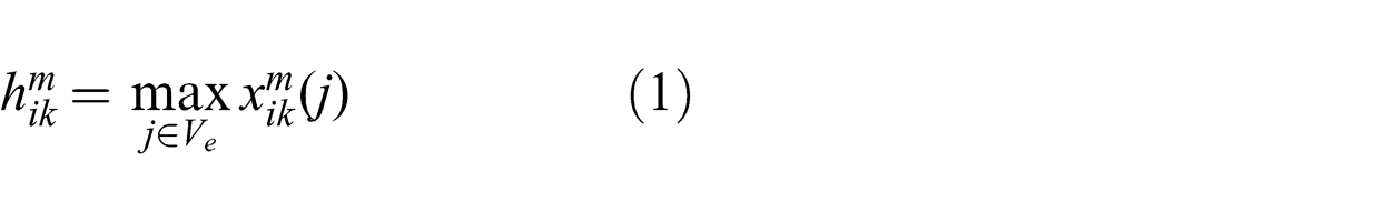
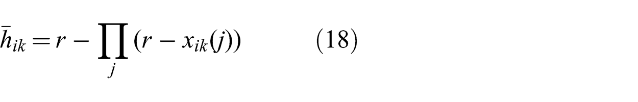
The chosen flow rates {x_ik (j)} are implemented using a multicast policy that determines how the inward flow of messages at a node is distributed amongst its children. In our problem formulation, we assume that network coding is used. For small-sized networks, network coding can introduce unnecessary complication with little performance advantage in practice (Keshavarz-Haddadt and Riedi, 2008). As an alternative, multicast routing can be implemented without network coding by using randomization. The probability of sending a given inward message along a given outward edge is set proportional to flow variable x_ik (j). In this case, the average total flow h_ik through the link for a source flow rate of r is given by (18) instead of the network coding relation given in (1):

h ¯ ik = r − Π j ( r − x ik ( j ) )

(18)

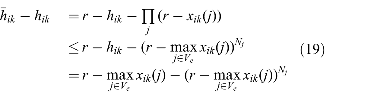
For a given set of flow variables, randomization will result in higher total flow through a link. The extra capacity required in comparison to network coding is given by the relation in (19). From the relation, we deduce that the gap is zero if the maximum flow variable over a link is equal to either zero or the source flow and that the gap is less significant when there are fewer destinations. Therefore, for ease of implementation we use randomization to implement the multicast policy. However, the total flow is still approximated by (1) since (18) otherwise leads to a non-convex problem. We found this approximation to be valid in practice:

h ¯ ik − h ik = r − h ik − Π j ( r − x ik ( j ) ) ≤ r − h ik − ( r − max j ∈ V e x ik ( j ) ) N j = r − max j ∈ V e x ik ( j ) − ( r − max j ∈ V e x ik ( j ) ) N j

(19)

To demonstrate the scalability of the algorithm, we performed an empirical study of the convergence time for a given set of link costs. This study, which gives a convergence time estimate, also gives further insight into the time required between link cost updates.

We evaluated the convergence time in min-cost-DIF through a simulated network using randomized but fixed link costs. Our simulated network includes one sensor and a variable number of processors and estimators where the number of processors is always one more than the number of estimators. Results of the simulation for an increasing number of nodes are shown in Figure 4. The convergence condition is satisfied when the change in the solution variables is below a certain threshold.

OPEN IN VIEWER

Fig. 4.

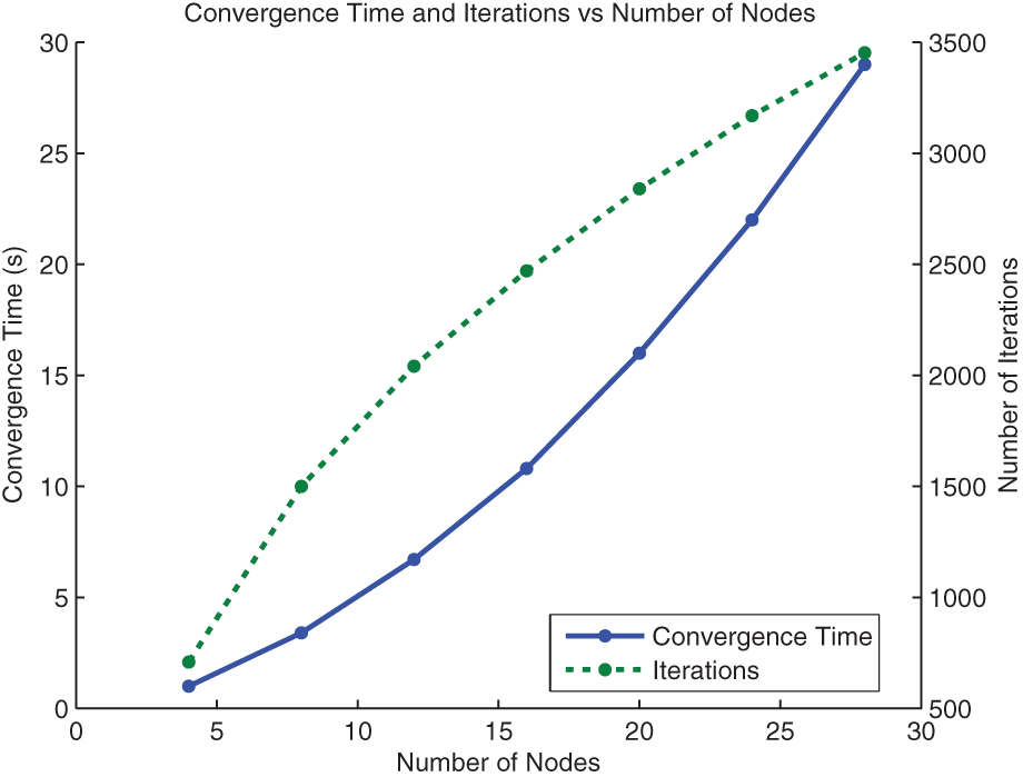
Convergence time and convergence iterations of the message passing optimization as a function of the number of nodes in a simulated network. The simulated network includes one sensor and an increasing number of processors and estimators where the number of processors is always one more than the number of estimators.

Convergence time depends both on the number of iterations required until convergence and the time expended in each iteration. The number of iterations to convergence is hardware-independent and the results shown in Figure 4 indicate that the number of iterations to convergence is a sub-linear function of the network size. The time required for each iteration involves computing routing updates and transmitting the updated values. The time complexity of the routing updates in (13) and (14) is polynomial in the size of the network. Transmission time, on the other hand, is typically linear in the size of the transmitted message which in turn is proportional to the size of the network.

The convergence times shown do not account for communication delay. To estimate such delay in practice, we observed from the experiments shown later in the paper (Sections 6.3 and 6.4) that the time for one iteration over wireless networks is typically less than 100 ms. This value corresponds to networks concurrently being utilized for transmission of sensor data and processed observations. Based on this estimate and the number of iterations at convergence, we can estimate typical values for convergence time for networks from five to ten nodes to be between 50 and 150 s.

This empirical analysis indicates that the running time of our algorithm is polynomial in the size of the network for typical problem instances of interest. We observed that the number of iterations required until convergence is sub-linear in the number of nodes, and the time complexity of each iteration is polynomial in the number of nodes. In practice, we found iteration times to be dominated by communication delay resulting in the convergence time indicated above. We envisage that this period can be reduced by employing various quality-of-service protocols, yet this solution is deferred to future work.

Based on the above analysis, we can now specify nominal values for the interval between link cost updates. The frequency of link cost updates is set such that the multicast routing algorithm has sufficient time to converge. In our implementation, we chose fixed values between 50 and 150 s. However, we note that while the optimization algorithm is iterating, a valid routing is available and information can continuously flow through the network. The frequency of link cost updates determines how reactive the algorithm is to changes in estimated sensor utility, and thus the importance of a higher update frequency would be to handle situations where sensor utility changes rapidly. We leave consideration of this case to future work.

4.4. Two-robot simulation

We evaluated our solution approach to min-cost-DIF in simulation for the case of two mobile robots tracking a moving target. The implementation is decentralized with nodes running in separate processes. The aim of this simulation is to demonstrate the multicast behavior of dynamic information flow and to show the improvement in information gain realized in the min-cost-DIF setting in comparison to a control condition with uniform-rate communication.

The simulation setup is shown in Figure 5. Two mobile robots are assigned to separate workspaces. The first robot has a 360° field-of-view sensor and the second robot has a 180° field-of-view sensor. The sensors are bearing-only sensors, forcing cooperation between the robots. A moving target tracked by the robots moves in a circular pattern within a square region of interest outside the robots’ workspaces.

OPEN IN VIEWER

Fig. 5.

Demonstration setting of the two-robot simulation and experiment. Robots 1 and 2 are shown with their boundaries. Sample target tracks are shown making a square pattern inside the region of interest.

The network diagram of the system is shown in Figure 6. The object detection routine on each robot imposes a processing cost. Due to the multicast property, the processing cost of each processing module is distributed among the receiving estimators. Therefore, if the estimators collectively evaluate an observation utility greater than the processing cost, then the sensor raw data should be processed and sent forward. Virtual links, not shown in the figure, allow for the no-send policy. The cost of the links incident onto the estimators is adjusted throughout the simulation by the robots’ sensor utility evaluations.

OPEN IN VIEWER

Fig. 6.

The min-cost-DIF network diagram for the two-robot simulation. Virtual links are omitted for clarity.

To validate the performance of the algorithm, a control test was also run. In the control test, the sensor rates were reduced to the same average rate used in the dynamic case.

The information for each of the robots’ estimate over time is shown in Figure 7 and the corresponding average bars are shown in Figure 8. In Figure 7(a), the information in Robot 1’s estimate was higher on average for the dynamic flow case. In contrast to the down-sampled case, the dynamic flow case boosted inter-robot flow when required preventing long periods of poor information gathering performance. The advantage of the dynamic flow case can also be seen more clearly in Figure 8(a). The dynamic case for Robot 2 exhibits some lag in information gathering performance but it eventually outperformed the down-sampled case as shown in Figure 7(b). This is also confirmed in Figure 8(b).

OPEN IN VIEWER

Fig. 7.

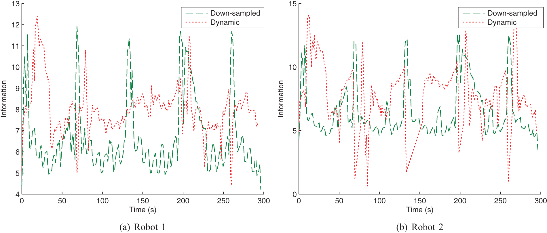
Information value (negative entropy) of the robots’ target estimate over time for the two-robot simulation. The plots are shown for two communication methods, down-sampled and dynamic, with both requiring the same amount of computation on average.

OPEN IN VIEWER

Fig. 8.

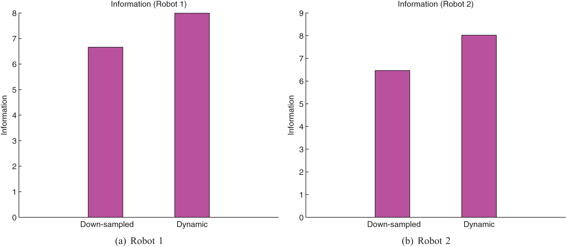
Time averages of the plots in Figure 7 shown in bar format. The improvement for the dynamic case over down-sampling is clearly observed.

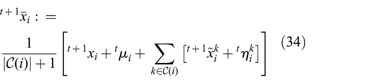
The policies and estimated sensor utilities for the dynamic flow case are plotted against time in Figure 9 with the corresponding averages shown in Table 2. The plots show consistency between sensor utility and flow. In particular, the oblique parts of the flow curve correspond to time periods where a robot would receive sensor observations freely due to raw data already being processed for the other robot. This free reception of data is a feature of multicast routing.

OPEN IN VIEWER

Fig. 9.

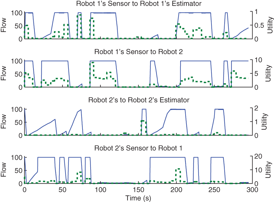
Flow rates and sensor utility for the two-robot simulation. Flow rates are shown in solid lines while the evaluated sensor utility is shown in dashed lines.

OPEN IN VIEWER

Table 2.

Average flow rates and Sensor Utility for the two-robot Simulation.

Link	Flow Rate	Sensor Utility
Robot 1’s sensor to Robot 1’s estimator	44.82	0.10
Robot 1’s sensor to Robot 2	55.03	1.64
Robot 2’s sensor to Robot 2’s estimator	26.12	0.04
Robot 2’s sensor to Robot 1	45.01	0.97

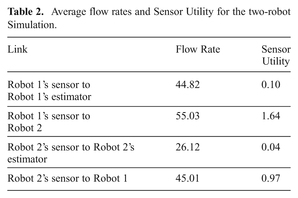
As noted in Section 4.3, discrete flow decisions minimize the error from our maximum flow approximation of the total flow in each link. As seen in Figure 9, with the exception of transient periods, the flow variables were mainly either 0 or 100.

4.5. Robot and ground station simulation

We also evaluated the case of one mobile robot and one ground station. The main purpose of this simulation is to show the generality of the dynamic information flow approach. The simulation was run using ROS and Gazebo.

The setting includes one Pioneer 2DX robot model with an on-board camera and one off-board processing station. The robot’s on-board processing is computationally expensive, however, it has wireless access to the off-board processing station. The demonstration process is as follows. The robot begins near the processing station. It then proceeds to gain information about a moving target.

The network diagram of the demonstration is depicted in Figure 10. Subject to communication cost, which is set proportional to distance, the robot’s decision is expected to vary between on-board and off-board processing. The maximum flow assumption is valid for this scenario since there is only one destination node.

OPEN IN VIEWER

Fig. 10.

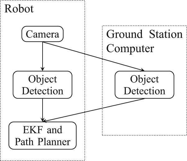
The min-cost-DIF diagram of the robot and ground station demonstration scenario.

Figure 11 shows the flow between the robot and the ground station, the communication cost and the robot’s processing cost over time. The processing cost is assumed to be fixed over time as shown in the figure. The communication cost varies based on the distance between the robot and the ground station and the flow is adjusted accordingly. In Figure 11, at around time step 50, communication cost outweighs the cost of on-board processing. This leads to a switch from off-board processing to on-board processing. It should be noted that the communication cost displayed in the plot is only for transmission from the sensor to the processor. When compared with on-board processing cost, the total communication cost is doubled. The results of this simulation show the generality of the dynamic flow formulation. Even though the expected behavior here is as expected, the aim is to show that this behavior was achieved within the min-cost-DIF framework without modification.

OPEN IN VIEWER

Fig. 11.

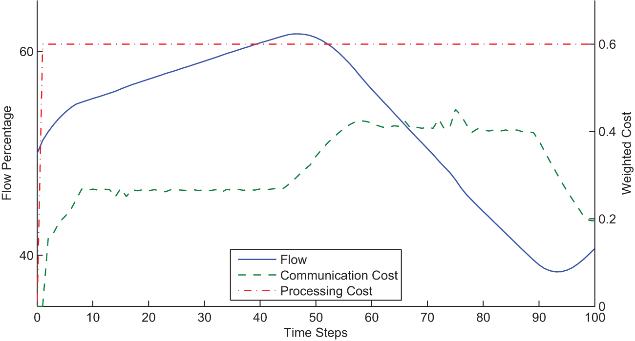
Flow, communication cost and processing cost of the link from the sensor to the ground station processor for the one robot/one ground station simulation.

4.6. Robot and ground station experiment

We also performed an experiment in hardware for the one robot/one ground station case. A Pioneer 3DX robot equipped with an on-board computer using an Intel Atom processor N270 1.6 GHz was used. The robot is equipped with a SICK LMS291 2D lidar used exclusively for localization. The robot uses an on-board webcam as a 2D bearing-only sensor to track a moving target. With the exception of the off-board processing ground station, all processes were executed on-board the robot including localization, image processing (when required), estimation, decision-making and the information flow control algorithm.

The change in flow, communication cost and processing cost over time is shown in Figure 12. These results are consistent with the simulation results for the analogous case. We observe that the robot initially chooses to send images to be processed off-board by the ground station. The ground station performs object detection and sends point observations back to the robot. As the robot moved away to track the target, the communication cost increased and thus the robot chose to perform processing on-board. A snapshot of the moment when the robot decided to switch to on-board processing is shown in Figure 13.

OPEN IN VIEWER

Fig. 12.

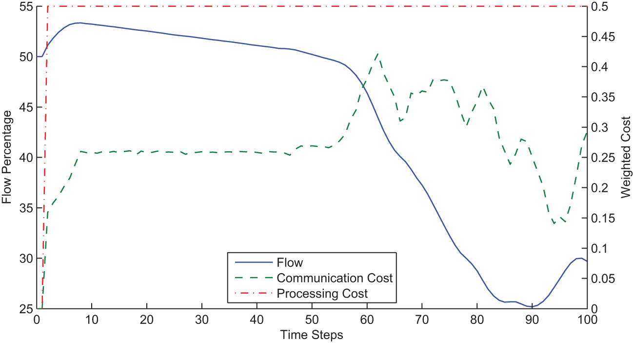
Experimental results for the one robot/one ground station case.

OPEN IN VIEWER

Fig. 13.

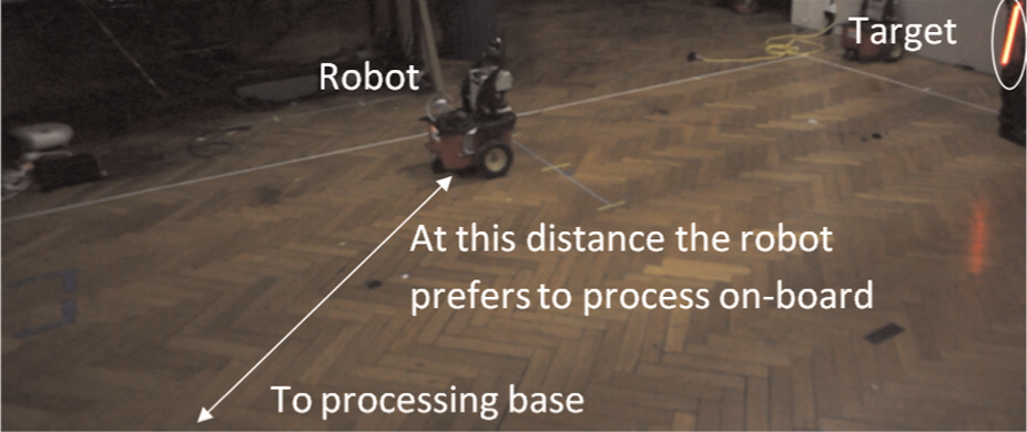
Snapshot from the one robot/one ground station experiment. The image shows the robot having moved away to follow the target. At this distance, the robot prefers to perform processing on-board.

4.7. Monte Carlo simulation

We performed a Monte Carlo simulation for the experimental setting of Section 4.4 comparing the down-sampled and the dynamic communication cases. The aim of the simulation is to analyze the statistical significance of the performance advantage introduced by our solution to min-cost-DIF.

Each method was tested in 20 randomly initialized trials running for 1 min each. The down-sampling rate was chosen to match the average rate resulting from the dynamic case.

The results of the Monte Carlo simulation are shown in Figure 14 in box-plot format. The results shown assume each trial as one sample. Dynamic communication clearly outperforms down-sampling. A Welch’s t-test for statistical significance resulted in a p-value of less than 0.001.

OPEN IN VIEWER

Fig. 14.

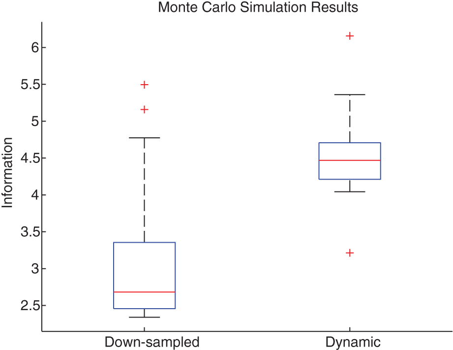
Monte Carlo simulation results comparing down-sampling with dynamic information flow. Each method was tested on the two-robot scenario for 20 trials running for 1 min each. In the results depicted, a trial acts as one sample. The box extents represent the first and third quartiles, while the whiskers represent the extrema. The median is represented by the horizontal line inside the box.

5.1 ADMM

For convenience, we provide a brief summary of ADMM. A detailed description can be found in Boyd et al. (2011).

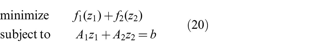
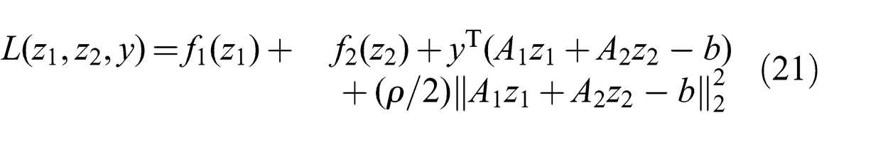
ADMM solves optimization problems of the form given by (20). The objective is assumed to be a sum of two proper convex functions f ₁ and f ₂ where the first is a function of the vector z ₁ and the other is a function of the vector z ₂. We refer to z ₁ as the primary vector variable and to z ₂ as the secondary vector variable. The Lagrangian of the problem is shown in (21):

minimize f 1 ( z 1 ) + f 2 ( z 2 ) subject to A 1 z 1 + A 2 z 2 = b

(20)

L ( z 1 , z 2 , y ) = f 1 ( z 1 ) + f 2 ( z 2 ) + y T ( A 1 z 1 + A 2 z 2 − b ) + ( ρ / 2 ) ‖ A 1 z 1 + A 2 z 2 − b ‖ 2 2

(21)

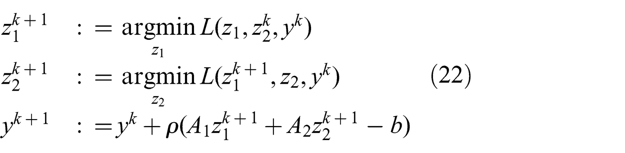
ADMM is summarized in (22). Each iteration involves three updates. The primary update minimizes the Lagrangian about z ₁, the secondary update minimizes the Lagrangian about z ₂ and the third updates the Lagrangian variable y. Convergence is shown in Boyd et al. (2011):

z 1 k + 1 : = argmin z 1 L ( z 1 , z 2 k , y k ) z 2 k + 1 : = argmin z 2 L ( z 1 k + 1 , z 2 , y k ) y k + 1 : = y k + ρ ( A 1 z 1 k + 1 + A 2 z 2 k + 1 − b )

(22)

5.2 Problem formulation

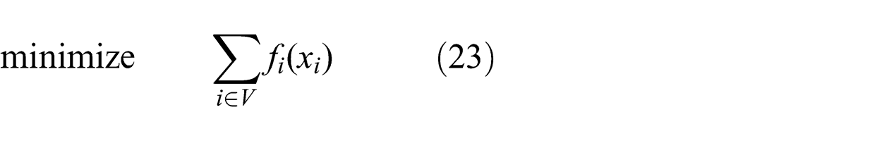
The general form of optimization problems that can be solved by DADMM is described as follows. Consider the DAG G = {V, E} defined in Section 3. Attach to each node i ∈ V a vector variable x_i and a proper convex function f_i (x_i ), which is not necessarily smooth. Node i can have constraints with its parents as per (24) where g_i is an affine function. The notation x_U where U = {i ₁,…,i_n }\subset V is defined as the concatenation of all vectors x_i such that i ∈ U, that is, x U = ( x i 1 , … , x i n ) . Function g_i is interpreted as a vector-valued function with its dimension indicating the number of constraints n g i . The goal of DADMM is to solve the optimization problem (23)–(24):

minimize ∑ i ∈ V f i ( x i )

(23)

subject to g i ( x i , x P ( i ) ) ) = 0 , ∀ i ∈ V

(24)

5.3 Inequality constraints

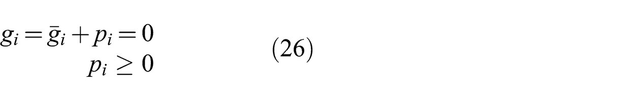
The standard form of ADMM does not include inequality constraints. Therefore, we have only included equality constraints g_i in the problem definition. This is a non-restrictive assumption since by adding extra variables, inequality constraints can be transformed into equality constraints as we will show. Suppose that instead of g_i we have a function g ¯ i that is required to satisfy the inequality constraint (25) instead:

g ¯ i ≤ 0

(25)

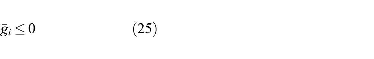
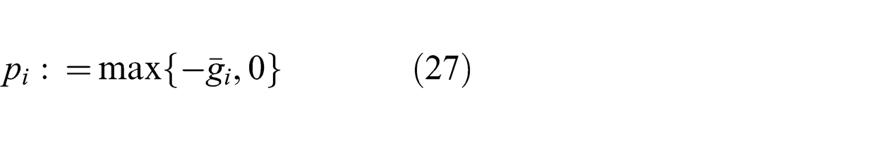
By adding a slack variable p_i , this inequality constraint becomes an equality constraint plus a non-negative constraint on p_i as shown in (26). The slack variable p_i can be viewed as a variable belonging to a virtual parent node whose objective is an indicator function that is zero when p_i is non-negative and infinity otherwise:

g i = g ¯ i + p i = 0 p i ≥ 0

(26)

In DADMM, p_i can be optimized independently. The solution of the optimization over p_i is given by (27):

p i : = max { − g ¯ i , 0 }

(27)

5.4 DADMM

DADMM consists of a preliminary decentralization step followed by the main optimization process. The decentralization step is only performed once during which the optimization problem is modified, through the addition of variables and constraints, such that it only requires neighbor-to-neighbor communication. In the optimization process, message passing and optimization updates run in a sequence that enforces decentralization while retaining equivalence to centralized ADMM.

The decentralization step modifies constraints (24). For every vector x_i where i ∈ V, a mirror vector x ¯ i is introduced. The vector x ¯ i acts as an interface for all other nodes. Any child node k that has a constraint including x_i replaces x_i with a local copy x ~ i k and an equality constraint between x ~ i k and x ¯ i is added. Symmetrically, from node i’s perspective x P ( i ) is replaced with x ~ P ( i ) . Therefore, from node i’s perspective, (24) is replaced with (28) to (30):

g i ( x i , x ~ P ( i ) i ) = 0

(28)

x i − x ¯ i = 0

(29)

x ~ P ( i ) i − x ¯ P ( i ) = 0

(30)

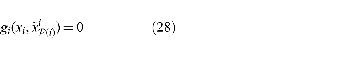
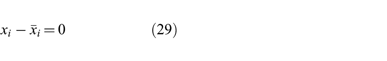
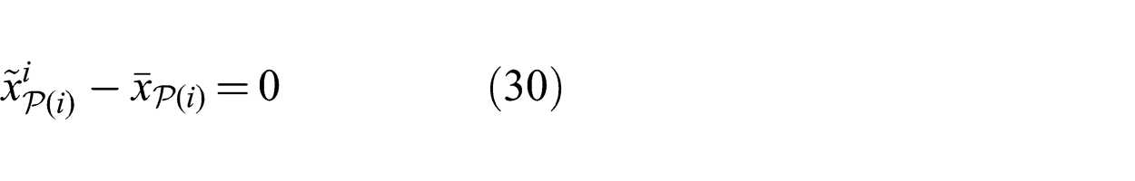
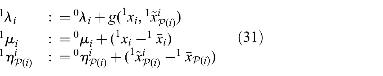
The new constraints are assigned the following Lagrangian multiplier vectors. The Lagrangian multiplier λ_i is associated with constraint (28), μ_i is associated with constraint (29) and η P ( i ) i is associated with constraint (30).

All the above constraints and variables except x ¯ P ( i ) are attached to node i. This means that x ¯ P ( i ) is node i’s only dependency on its parent nodes and x ¯ i is the interface variable that is shared with node i’s children. We note that constraint (28) is now an internal constraint. This decentralization has decoupled the parents of node i. The decoupling is evident by noting that (30) is a decoupled set of equality constraints: x ~ l i = x ¯ l , ∀ l ∈ P ( i ) . The decentralization step is shown schematically in Figure 15.

OPEN IN VIEWER

Fig. 15.

Decentralization step of DADMM. In (a), node i is shown with its parents and children in a DAG. It is assumed that node i has constraints that include all of its parents. By transforming the network into that of (b), each of node i’s parents only needs to communicate with node i given that they are not coupled elsewhere.

From the ADMM perspective, the sets of vector variables x_i and x ~ P ( i ) i are mapped to z ₁ in (20) and the sets of variables x ¯ i are mapped to z ₂. The sets of constraints (28) to (30) are collectively mapped to the equality constraint in (20). Define x ^ i = ( x i , x ~ P ( i ) i ) . Based on the mapping to ADMM, x ^ i is the primary vector variable while x ¯ i is the secondary vector variable.

The main optimization process consists of message passing and optimization updates defined in a sequential and decentralized manner that is equivalent to the centralized version (22). The process begins with the head nodes and then proceeds to traverse the graph according to Algorithm 1. Algorithm 1 refers to two types of updates and two types of messages, upward and downward. We will now proceed to define what takes place during each update and what each message contains.

At the outset, each node i ∈ V is initialized with¹ x_i , 1 x ¯ i , 1 x ~ P ( i ) i ,⁰ λ_i ,⁰ μ_i and 0 η P ( i ) i . In the tth downward update, node i updates its Lagrangian multipliers to obtain ^t λ _i , ^t μ _i and t η P ( i ) i . It then updates the primary variables to obtain ^t+1 x_i and t + 1 x ~ P ( i ) i . The node’s downward message contains t x ¯ i that is required by its children nodes to update their primary variables. In the tth upward update node i updates its secondary variables to obtain t + 1 x ¯ i . It then sends its upward message containing variables t + 1 x ~ P ( i ) i and Lagrangian multipliers t η P ( i ) i .

The decentralized nature of the process is evident from the definition of the updates at the node level. We need to show that the process is in fact equivalent to performing the centralized version of ADMM on the entire system. A proof of this equivalence is provided in Theorem 2 following Lemma 2.

Lemma 2. In Algorithm 1, every downward update t of node i is followed by an upward update t. Moreover, every upward update t of node i is followed by a downward update t + 1.

Proof. From Lemma 1, we know that if node i has just performed the tth update then it has performed t − 1 upward updates. Now, suppose that the next update is the (t + 1)th downward update. This is impossible because according to Lemma 1, node i would have performed t upward updates. The second part of the statement can be proved through a similar argument.

Theorem 2. For each node i, after the t-th update of the Lagrangian multipliers in the downward update, the variables owned by the node are equal to the ADMM update t of those variables.

Proof. The proof is by induction. Before the start of the algorithm, the variables of node i are set to¹ x_i , 1 x ¯ i , 1 x ~ P ( i ) i ,⁰ λ_i ,⁰ μ_i and 0 η P ( i ) i . During the first downward update, node i’s Lagrangian variables are updated according to (31). The node would have received 1 x ¯ P ( i ) from its parents’ downward messages. At this stage, all variables belong to the ADMM update at t′ = 1:

1 λ i : = 0 λ i + g ( 1 x i , 1 x ~ P ( i ) i ) 1 μ i : = 0 μ i + ( 1 x i - 1 x ¯ i ) 1 η P ( i ) i : = 0 η P ( i ) i + ( 1 x ~ P ( i ) i - 1 x ¯ P ( i ) )

(31)

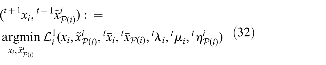
Assume that after node i’s (t − 1)th Lagrangian update, all variables belong to the ADMM update at t′ = t − 1. We now prove the statement for t′ = t. After the (t − 1)th Lagrangian variable update, node i directly updates its primary variables according to (32):

( t + 1 x i , t + 1 x ~ P ( i ) i ) : = argmin x i , x ~ P ( i ) i L i 1 ( x i , x ~ P ( i ) i , t x ¯ i , t x ¯ P ( i ) , t λ i , t μ i , t η P ( i ) i )

(32)

According to Lemma 2, the downward update is followed by an upward update. In the upward update, node i would have received t + 1 x ~ i C ( i ) from its children as well as the corresponding Lagrangian variables t η i C ( i ) . After receiving these variables, node i updates the secondary variables according to (33):

t + 1 x ¯ i : = argmin x ¯ i L i 2 ( t + 1 x i , t + 1 x ~ i C ( i ) , x ¯ i , t − 1 μ i , t η i C ( i ) )

(33)

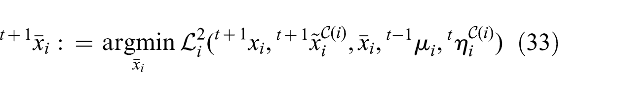
The minimization over x ¯ i can be written explicitly as shown in (34):

t + 1 x ¯ i : = 1 | C ( i ) | + 1 [ t + 1 x i + t μ i + ∑ k ∈ C ( i ) [ t + 1 x ~ i k + t η i k ] ]

(34)

Finally, from Lemma 2, we have given that the upward update is followed by downward update t + 1 during which the Lagrangian variables are updated in an analogous manner to (31) to obtain ^t+1 λ_i , ^t+1 μ_i and t + 1 η P ( i ) i . Hence, the (t + 1)th ADMM update is complete.

5.5. Analysis

In this section, we analyze the computational complexity of one iteration of DADMM. Analysis of the full problem depends on its convergence rate, which we consider for the special case of threshold-DIF in Section 6.

First, we define the following terms:

n g i : number of constraints for node i n g max : = max i ∈ V n g i n i : = | x i | = | x ¯ i | n ′ i : = | x ~ P ( i ) i | n max : = max i ∈ V n i

(35)

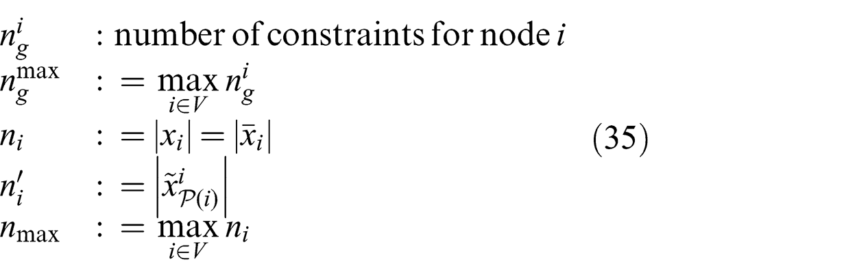
The worst-case complexity of one iteration of DADMM is given by Theorem 3.

Theorem 3. Each iteration of DADMM over a DAG G = {V, E} runs in O ( κ ( G ) ( n max | V | ) 2 ( n g max + n max | V | ) ) time.

Proof. Each ADMM iteration consists of three updates: the primary update, secondary update and the Lagrangian update. Since the algorithm is decentralized and synchronous, its running time is dominated by the time to update a single node multiplied by the depth of G.

We now develop an upper bound on the computation performed by an arbitrary node i. The primary update involves solving ∇ x ^ i L = 0 . This equation is a linear equation, since the Lagrangian is quadratic and has the form A x ^ i = d , where A ∈ ℝ ( n i + n ′ i ) 2 and d ∈ ℝ n i + n ′ i since the primary vector x ^ i has dimension equal to n_i  + n′ _i . Each element in A potentially contains a term from the objective and a term from each constraint in which the corresponding element in x ^ i is involved. Each element of x ^ i is involved in an equality constraint (with the secondary variables) and may appear in the constraints of g_i . Therefore, the elements of A can be computed in O ( ( n i + n ′ i ) 2 ( 2 + n g i ) ) = O ( ( n i + n ′ i ) 2 n g i ) time. Each element in d can include a secondary variable and a Lagrangian multiplier from each constraint. The time complexity of computing the elements of d is O ( ( n i + n ′ i ) ( 1 + n g i ) ) . Solving for x ^ i , assuming a dense matrix A, takes O ( ( n i + n ′ i ) 3 ) time. Therefore, the time complexity of the primary update is O ( ( n i + n ′ i ) 2 ( n i + n ′ i + n g i ) ) .

The secondary update computes an average over x_i and x ~ i C ( i ) to obtain x ¯ i . Thus, its time complexity is O ( n i ( 1 + | C ( i ) | ) ) = O ( n i | C ( i ) | ) .

The Lagrangian update involves an evaluation of all constraints given by equations (28), (29) and (30). The evaluation of each element of g_i involves at most n_i  + n′ _i variables. The evaluation of the other constraints involves two variables each. Therefore, the time complexity of the Lagrangian update is O ( n g i ( n i + n ′ i ) + n i + n ′ i ) = O ( n g i ( n i + n ′ i ) ) .

The total time complexity is the sum of these three updates. Thus, we have O ( ( n i + n ′ i ) 2 ( n i + n ′ i + n g i ) ) + O ( n i | C ( i ) | ) + O ( n g i ( n i + n ′ i ) ) = O ( ( n i + n ′ i ) 2 ( n i + n ′ i + n g i ) + n i | C ( i ) | ) .

We now restate the bound as a function of n _max, n g i and |V|. Since n _max is an upper bound for n_i , n max | P ( i ) | is an upper bound on n′ _i . An upper bound for the number of children or the number of parents is simply the number of nodes |V|. Hence, a more conservative upper bound for n′ _i is n _max|V|. Therefore, the overall time complexity for the work performed by node i can be rewritten as O ( ( n max | V | ) 2 ( n g max + n max | V | ) ) . The total time complexity for one iteration of the algorithm is thus O ( κ ( G ) ( n max | V | ) 2 ( n g max + n max | V | ) ) .

6.1. Threshold-DIF using DADMM

The threshold-DIF problem can be solved using DADMM. However, we first must reformulate constraints (4) and (7) such that they are compatible with the DADMM framework.

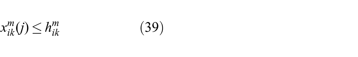
The maximum function in (4) is replaced by the set of inequalities (39). The maximum function is non-smooth and cannot be optimized in one step. With the set of inequalities in (39), the objective and all equality and inequality constraints of the optimization become linear as required by DADMM.

The set of inequalities in (39) is equivalent to the maximum relation in (4) as long as one of the constraints is active. One constraint will always be active for h ik m if the link cost c ik m is positive. From the problem formulation, we know that the link cost c ij m can only be negative if j ∈ V_e , that is, if the link is incident to an estimator j. For these links, we replace the set of inequalities in (39) with the set of equalities given in (36):

x ik m ( j ) = 0 , if k ≠ j x ik m ( j ) = h ik m , if k = j

(36)

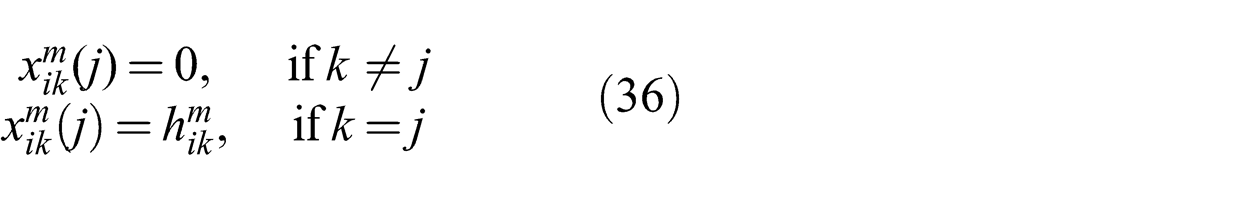
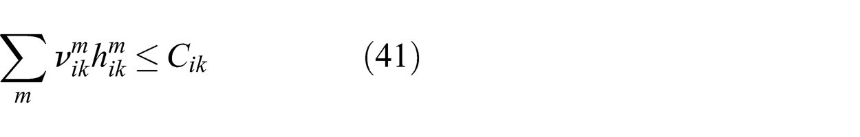
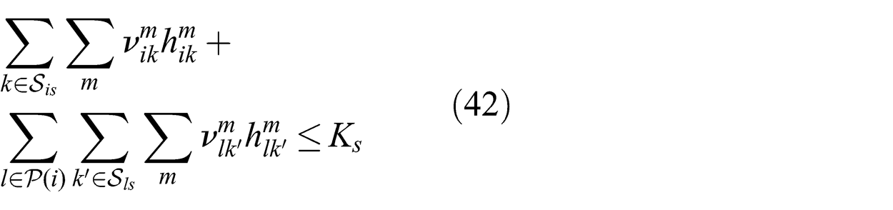
The inter-link constraint (7) is replaced by (42) where S is is the set of links emanating from node i involved in the inter-link constraint s. The DADMM format only permits constraints between a node and its parents. Therefore, constraint (42) only applies between links from node i and links from node i’s parents. This condition is not restrictive since an extra link can be added between non-neighboring nodes with inter-link constraints while retaining the directed acyclic property of the graph. The graph remains acyclic by preserving any ordering between the two nodes between which the extra link is added. Since the network is a connected DAG, then, by definition, for any two nodes i and k either k is a successor of node i, k ∈ C ¯ ( i ) or k is an ancestor of i, k ∈ P ¯ ( i ) or neither. If k ∈ C ¯ ( i ) , the link should extend from i to k. If k ∈ P ¯ ( i ) , the link should extend from k to i. If there is no directed path between the nodes, then either direction retains the acyclic property.

After transforming the constraints, we obtain the problem (37)–(42) shown below:

minimize ∑ ( i , k ) ∈ E c ik m h ik m

(37)

subject to x ik m ( j ) ≥ 0

(38)

x ik m ( j ) ≤ h ik m

(39)

∑ l ∈ P ( i ) x li m ( j ) − ∑ k ∈ C ( i ) x ik m ( j ) + r i m ( j ) = 0

(40)

∑ m ν ik m h ik m ≤ C ik

(41)

∑ k ∈ S is ∑ m ν ik m h ik m + ∑ l ∈ P ( i ) ∑ k ′ ∈ S ls ∑ m ν lk ′ m h lk ′ m ≤ K s

(42)

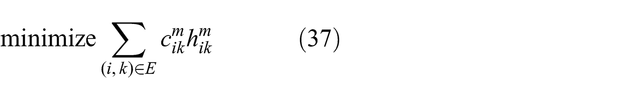
To solve threshold-DIF, all that is required at this stage is that the threshold-DIF variables and constraints be mapped to the variables of the distributed optimization problem (23)–(24). This can be done as follows. The sets of variables { h ik m : m ∈ V s , k ∈ C ( i ) } and { x ik m ( j ) : m ∈ V s , j ∈ V e , k ∈ C ( i ) } are mapped to x_i . The objective function f_i in (23) is represented by ∑ k ∈ C ( i ) ∑ m c ik m h ik m and the indicator functions resulting from the inequality constraints. The constraint g_i in (24) is represented by the equality constraints and the equality versions of the inequality constraints involving node i in (37) to (42).

DADMM runs continuously throughout system operation. As the system configuration changes, link costs and weights are updated with new values. To ensure convergence, the interval between updates is set to an adequate time period. In practice, this interval was found to be of similar length to that of min-cost-DIF in Section 4.3.

6.2. Analysis

In this section, we provide time complexity analysis of DADMM when applied to threshold-DIF. The complexity is expressed in terms of the size of the threshold-DIF input parameters.

Complexity analysis is provided for the entire optimization process including the number of iterations required for convergence. We first determine the complexity of one iteration following directly from Theorem 3. We then find a bound on the number of iterations based on the algorithm’s convergence rate.

The complexity of a DADMM iteration was determined in Section 5.2. The complexity of one iteration in terms of threshold-DIF problem specification can be determined by substituting the appropriate values for n _max and n g max . To begin, we denote the number of sources, destinations and inter-link constraints in the network as follows:

The maximum number of primary variables n _max is proportional to the maximum number of routing variables which, in turn, is proportional to the number of sources multiplied by the number of destinations multiplied by the number of children. The number of children is bounded from above by the number of nodes. Therefore, n _max is bounded such that n _max ≤ N_mN_j |V|.

The maximum number of constraints n g max is bounded by the maximum number of flow consistency constraints (40) and the maximum number of inter-link constraints (42). The number of consistency constraints is proportional to the number of sources multiplied by the number of destinations. Therefore, n g max is bounded such that n g max ≤ N m N j + N s .

Substituting the obtained bounds into the result of Lemma 3, the complexity of one iteration of DADMM for threshold-DIF becomes O ( κ ( G ) ( | V | 2 N m N j ) 2 ( | V | 2 N m N j + Ns ) ) . In threshold-DIF, the depth of the underlying graph is a function of processor cascading which is independent of the number of robots. Therefore, the depth is assumed to be constant. Hence, the time complexity of one iteration can be restated as O ( ( | V | 2 N m N j ) 2 ( | V | 2 N m N j + Ns ) ) .

To determine the complexity of the whole optimization process, the convergence rate is required. A convergence rate in an ergodic sense is established in He and Yuan (2012) with relatively mild assumptions.

The result is restated here after establishing the appropriate notation. Define the primal vector of the kth iteration as z k = ( z 1 k , z 2 k ) where z 1 k and z 2 k are the ADMM primary and secondary vectors defined in Section 5.1. Define the ergodic average z ~ k = ∑ k ′ = 1 k + 1 z k ′ and define z* and y* as the optimal primal and dual vectors. Then, if we assume that z ⁰ = 0 and y ⁰ = 0, the convergence result is given by (43). The positive constants α and β are independent of the dimension and value of both the primal and dual variables:

L ( z ~ k , y * ) − L ( z * , y * ) ≤ α ‖ z * ‖ 2 + β ‖ y * ‖ 2 ( k + 1 )

(43)

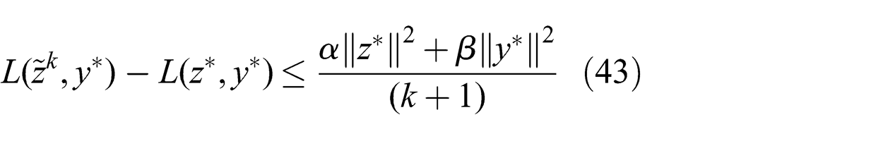
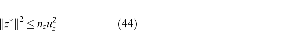
From (43), it is clear that in order to obtain a bound on the convergence rate, we need to find an upper bound on the squared norm of the primal and dual optimal vectors. The absolute value of the elements in the primal vector have an upper bound u_z which follows from the problem definition in Section 6.1. Hence, an upper bound on the norm of the primal vector is given by (44):

‖ z * ‖ 2 ≤ n z u z 2

(44)

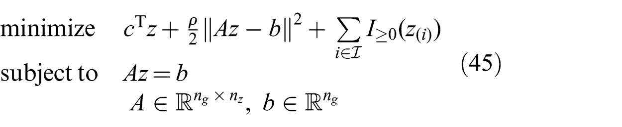
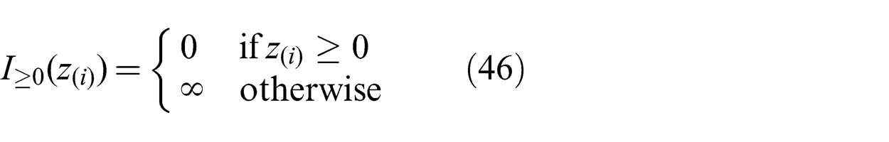
We now seek a bound for the squared norm of the dual vector ‖y*‖². To simplify the analysis, we note that the centralized ADMM version of the threshold-DIF problem has the form of the optimization problem defined in (45) where the indicator function I _≥0 is defined in (46) below. The set I contains the indices of the variables added to convert any inequality constraint into an equality constraint as described in Section 5.2. These variables need to satisfy the inequality constraint z _(i) ≥ 0 and they only appear in one row of the set of equality constraints Az = b:

minimize c T z + ρ 2 ‖ Az − b ‖ 2 + ∑ i ∈ I I ≥ 0 ( z ( i ) ) subject to Az = b A ∈ ℝ n g × n z , b ∈ ℝ n g

(45)

I ≥ 0 ( z ( i ) ) = { 0 if z ( i ) ≥ 0 ∞ otherwise

(46)

An upper bound on ‖y*‖² can be obtained from the following lemma.

Lemma 3. Assume that the equality constraints and the inequality constraints z_i  ≥ 0 active at x*are all linearly independent. Then, there exists a positive constant γ independent of z, n_z and n_g such that ‖y*‖² ≤ γ‖c‖².

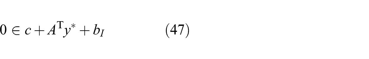
Proof. At optimality, we have Az − b = 0 and zero belongs to the subdifferential of the Lagrangian as shown in (47). The ith element of the vector b I ∈ ℝ n z is defined in (48) where ∂I _≥0 is the subgradient of the non-smooth indicator function:

0 ∈ c + A T y * + b I

(47)

b ( i ) = { ∂ I ≥ 0 if i ∈ I and the constraint z i ≥ 0 is active 0 otherwise

(48)

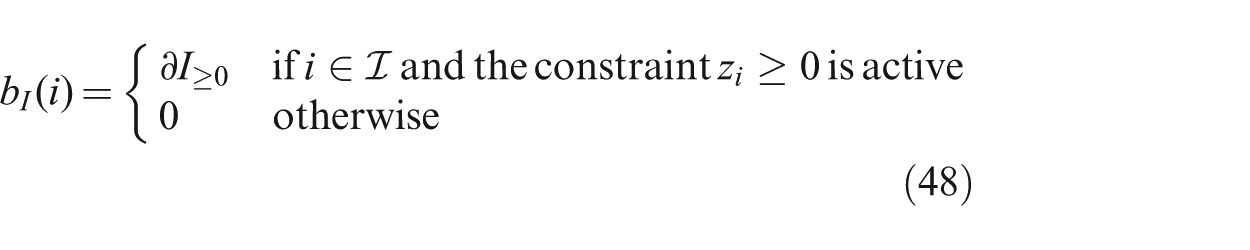
The subgradient ∂I _≥0 evaluated at 0 is an unbounded set and therefore cannot be used to directly bound y*. However, the optimality condition (47) has n_z rows while y* has dimension n_g . Furthermore, the maximum number of active inequality constraints, that is, constraints where b ( i ) ≠ 0 , is equal to (n_z  − n_g ) since otherwise x* would be over-defined by the constraints due to the linear independence assumption. Consequently, if all rows in (47) such that b ( i ) ≠ 0 are removed, there will remain at least n_g rows.

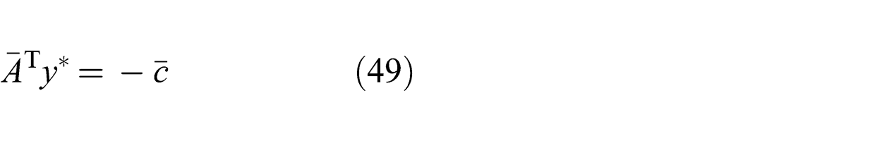
To this end, we need to make sure that the matrix A ¯ T obtained after removing the rows from A ^T remains full rank. When active, the inequality constraint z _(i) ≥ 0 becomes z _(i) = 0. If this equality is augmented as a row vector to the matrix A, due to the linear independence assumption, the rank of A becomes n_z  + 1. Through elementary row operations, any non-zero element on the column corresponding to z _(i) can be changed to zero with no change in the rank of the matrix. At this stage, the row z _(i) = 0 can then be removed with the rank of the matrix dropping back to n_g . Once the row is removed, the column corresponding z _(i) column is now all zeros and can hence be removed with no change in rank. This proves that A ¯ T has full rank n_g .

Therefore, the optimality condition (47) can be restated as (49) where c ¯ is the vector obtained after removing all the corresponding rows from c. The vector b_I becomes a zero vector after removing these rows:

A ¯ T y * = − c ¯

(49)

From (49), we obtain (50) where σ min ( A ¯ A ¯ T ) is the minimum eigenvalue of A ¯ A ¯ T and is greater than zero since A ¯ is full rank:

‖ c ¯ ‖ 2 ‖ y * ‖ 2 = y * T A ¯ A ¯ T y * ‖ y * ‖ 2 ≥ σ min ( A ¯ A ¯ T )

(50)

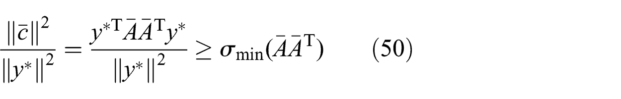
The proof is established by setting γ = 1 / σ min ( A ¯ A ¯ T ) and noting that ‖ c ¯ ‖ 2 ≤ ‖ c ‖ 2 since c ¯ is obtained by removing elements from c.

We assume that all elements in c are upper-bounded by a constant value u_c . This is a reasonable assumption since c represents the link cost vector and only the relative cost is of importance. Consequently, from Lemma 3, we have the upper bound given in (51) for the squared norm of the dual vector:

‖ y * ‖ 2 ≤ γ u c 2 n g

(51)

We can now state the main complexity result given by Theorem 4. The complexity is polynomial as expected since the problem is convex and the number of variables is polynomial in the number of nodes.

Theorem 4. Obtaining an ε-optimal solution for the threshold-DIF problem using DADMM has a computational complexity of O ( ( | V | 2 N m N j ) 2 ( | V | 2 N m N j + N s ) ( | V | 3 N m N j + N s ) / ϵ ) .

Proof. Bounds (44) and (51) mean that the left-hand side of (43) is bounded by a constant weighted sum of n_z and n_g . Therefore, an upper bound on the number of iterations k required to produce an error ε is given as O ( ( n z + n g ) / ϵ ) .

Note that the number of primary variables n_z is bounded by O ( | V | 2 N m N j ) multiplied by the number of nodes. Therefore, we have n z ≤ O ( | V | 3 N m N j ) . The number of constraints n_g , on the other hand, can be bounded such that n g ≤ O ( | V | 3 N m N j + N s ) . Thus, the resulting number of iterations of the optimization process is given by (52):

k ≤ O ( ( | V | 3 N m N j + N s ) / ϵ )

(52)

The complexity of the whole optimization process is obtained by multiplying the number of iterations by the complexity of each iteration. Thus, for an ε-optimal solution, DADMM for threshold-DIF runs in O ( ( | V | 2 N m N j ) 2 ( | V | 2 N m N j + N s ) ( | V | 3 N m N j + N s ) / ϵ ) time.

6.3. Two-robot experiment

We implemented our approach and performed an experiment where two mobile robots communicate to track a moving target. The aim of this experiment is to show the information gain advantage of dynamic information flow in the case of limited inter-robot communication bandwidth.

6.3.1. Experimental setup:

The experimental system consists of two modified Segway RMP 400 robots. An image of the robots is shown in Figure 16. The first robot is equipped with a Velodyne 3D Lidar with a 360° field of view. The second robot is equipped with a 2D SICK LMS291 horizontally mounted laser scanner with a 180° field of view. Although these sensors provide range as well as bearing, they were treated as bearing-only sensors to force cooperation between the robots. Each robot is also equipped with a server-class computer with an eight-core processor. For localization, the two robots rely on high-accuracy inertial measurement unit (IMU) and differential global positioning system (DGPS) modules.

OPEN IN VIEWER

Fig. 16.

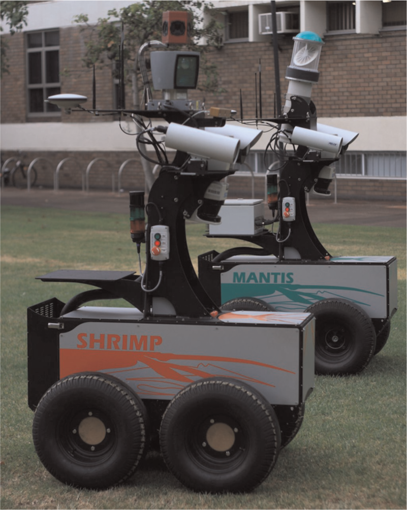
The Segway RMP 400 robots used in the experiments.

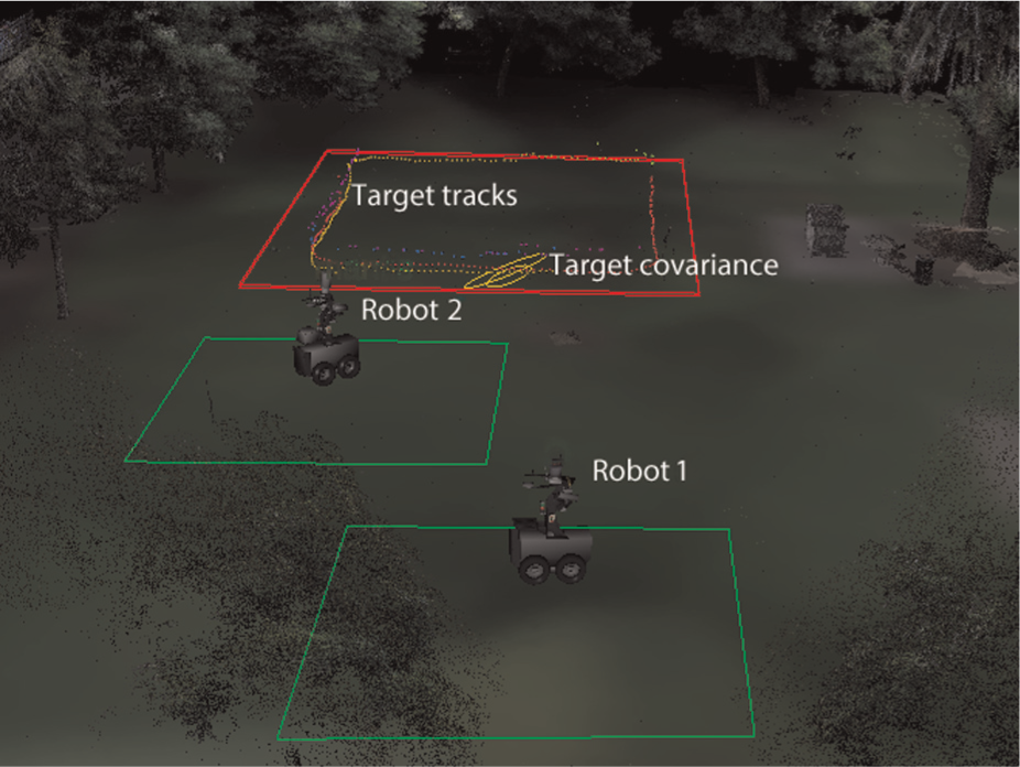
An image of the experimental setting is shown in Figure 17. The two robots were placed in two separate areas with virtually bounded geographical regions to avoid collision. Target tracking was limited to a geographically bounded region of interest and for the purpose of the demonstration, tracking was limited to one target performing circular patterns.

OPEN IN VIEWER

Fig. 17.

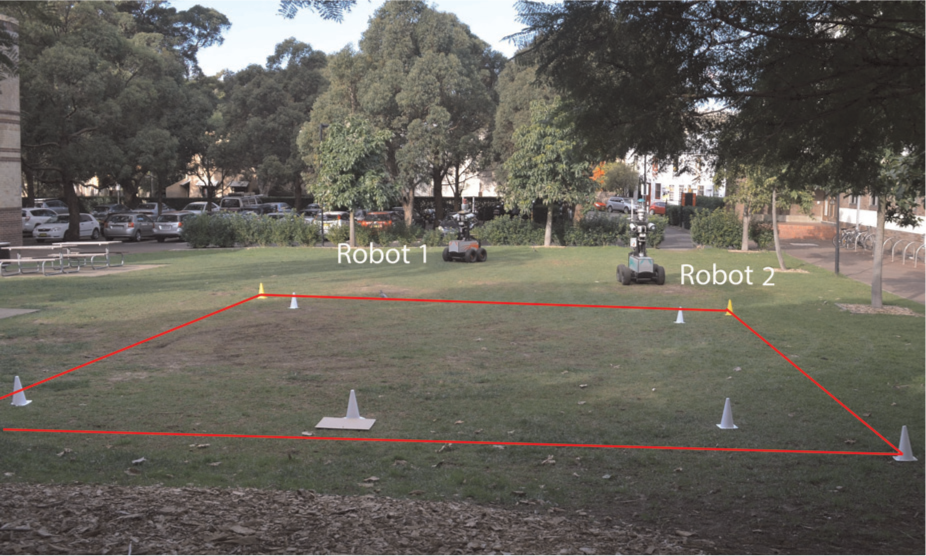
The outdoor experimental setup, with robots visible outside the tracking region of interest. The border of the tracking region is designated by solid lines.

The network diagram for this demonstration is shown in Figure 18. It is assumed that maximum communication bandwidth is limited and does not allow both robots to send sensor data at the full rate. We also assume that communication throughput decreases with inter-robot distance. Therefore, the robots are required to share the available bandwidth. The bandwidth sharing constraint is indicated by the dashed lines drawn between the two inter-robot links. Virtual links, not shown in the figure, allow for the no-send decision. It is expected that through dynamic information flow the bandwidth will be shared efficiently with respect to sensor utility. The maximum flow assumption is valid in this scenario since no processing costs are assigned.

OPEN IN VIEWER

Fig. 18.

The threshold-DIF diagram for the two-robot scenario. Virtual links are omitted for clarity.

To validate the performance of dynamic information flow, two control tests were run for the purpose of comparison. The first control test allows unconstrained communication between all nodes and shall be referred to as the unconstrained case. This test mainly acts as a benchmark since it violates bandwidth constraints. The second control test involves a reduced communication rate that obeys bandwidth bounds. This test shall be referred to as the down-sampled case.

6.3.2. Results:

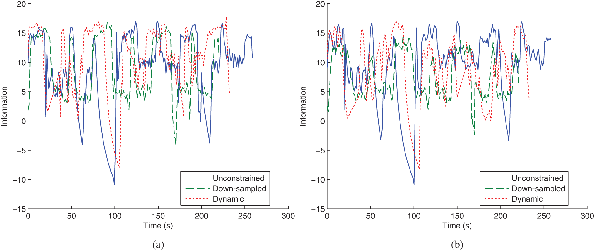
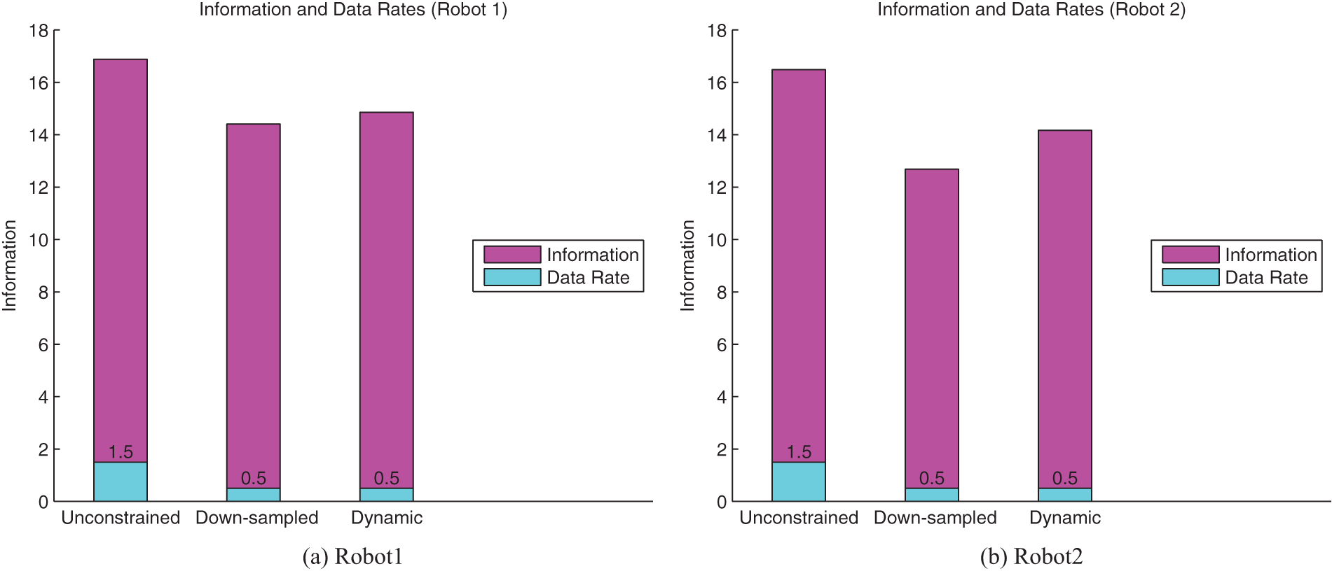
The information value for the robots’ target estimates over time is shown in Figure 19 with the corresponding average bars shown in Figure 20. In both figures, we observe minimal difference in information value across the three communication methods for Robot 1. Because Robot 1 has a 360° field-of-view sensor, the target is always visible and therefore tracking does not depend on observations received from Robot 2. However, we do observe a difference in information value for Robot 2. Figure 20(b) shows that the down-sampled method results in reduced information gathering performance when compared to our method. This effect is also evident in Figure 19(b) where there is a clear decline in information for the down-sampled case at times 20 s and 60 s. This decline occurs because the target drops outside the robot’s sensor field-of-view. Dynamic flow ensured that information was directed from Robot 1 to Robot 2, but down-sampling naively shared the communication medium.

OPEN IN VIEWER

Fig. 19.

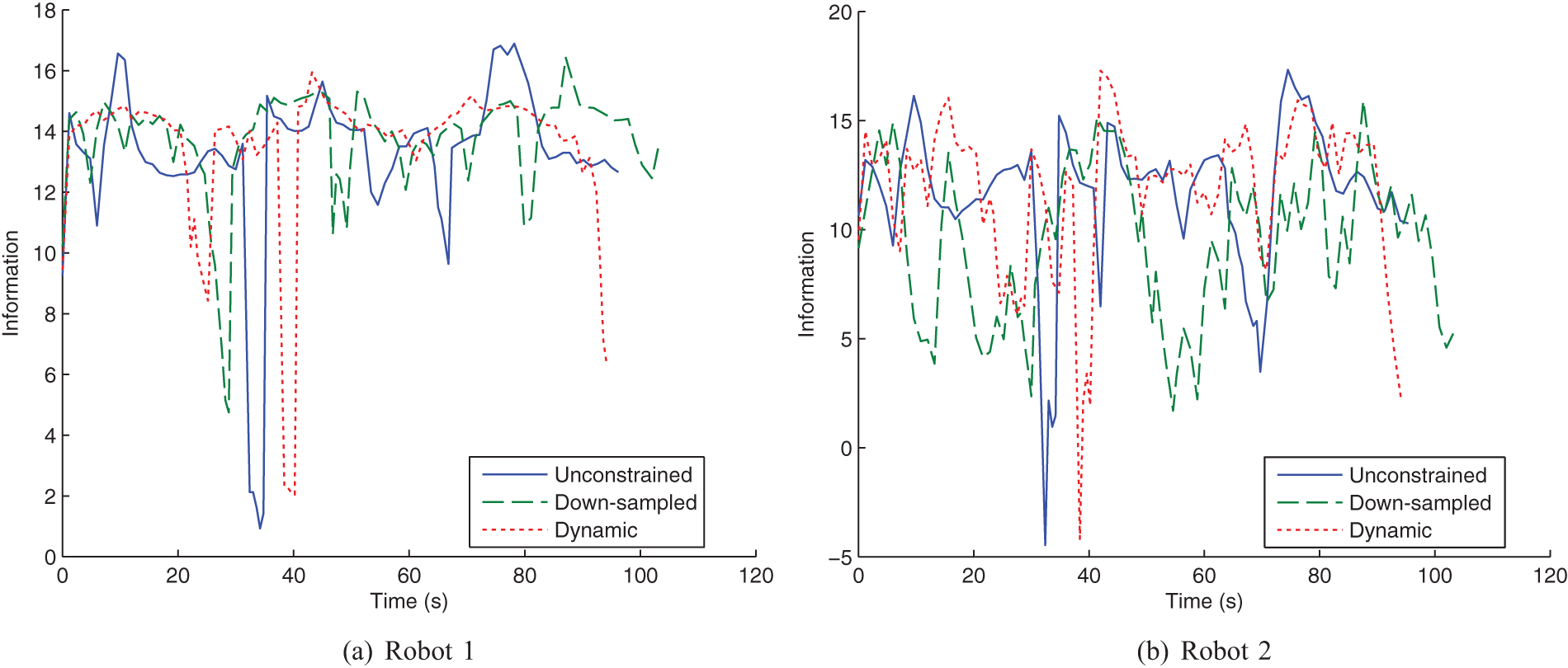
The information value (negative entropy) of the robots’ target estimate for the two-robot hardware experiment. Plots shown are for all three communication methods: unconstrained, down-sampled and dynamic. The sudden drops in information are due to target loss.

OPEN IN VIEWER

Fig. 20.

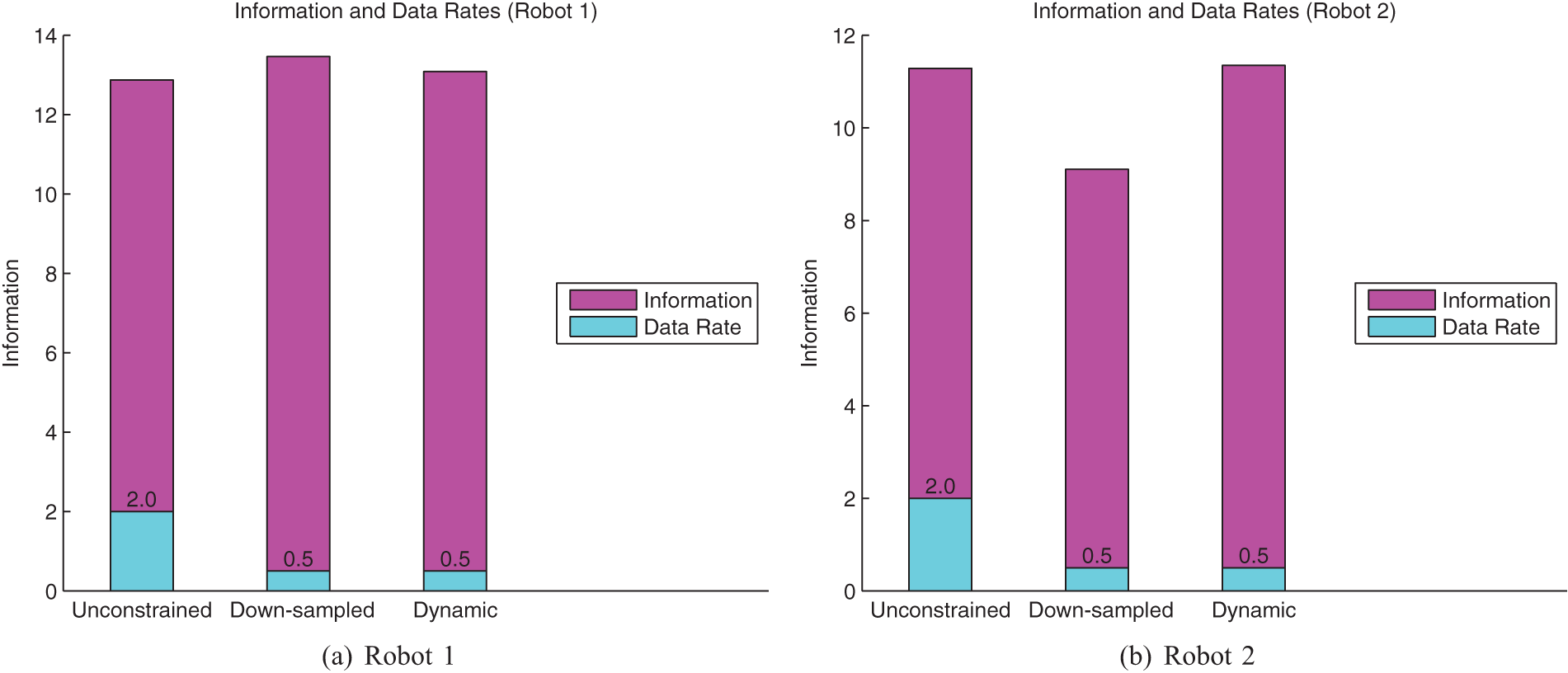
Time averages of the plots in Figure 19 shown in bar format. Data rates are shown superimposed. The dynamic case shows a clear improvement in information gain in comparison to down-sampling for Robot 2.

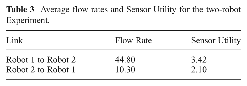
The advantage of dynamic information flow is further confirmed in Figure 21. The bottom two plots show the approximate sensor observation utilities and data flow between robots over time for the dynamic flow case. The flow from Robot 1 to Robot 2 dominates bandwidth usage when the target is not in Robot 2’s sensor field-of-view. However, at times 40 s and 80 s, the flow was directed from Robot 2 to Robot 1 because the target was closer to Robot 2. The top plot shows the distance between the robots over time. At the average inter-robot distance, the available bandwidth is limited to approximately half of the maximum bandwidth. As expected, the sum of the information flows obeys this reduced capacity. The flow rate and sensor utility averages are shown in Table 3.

OPEN IN VIEWER

Fig. 21.

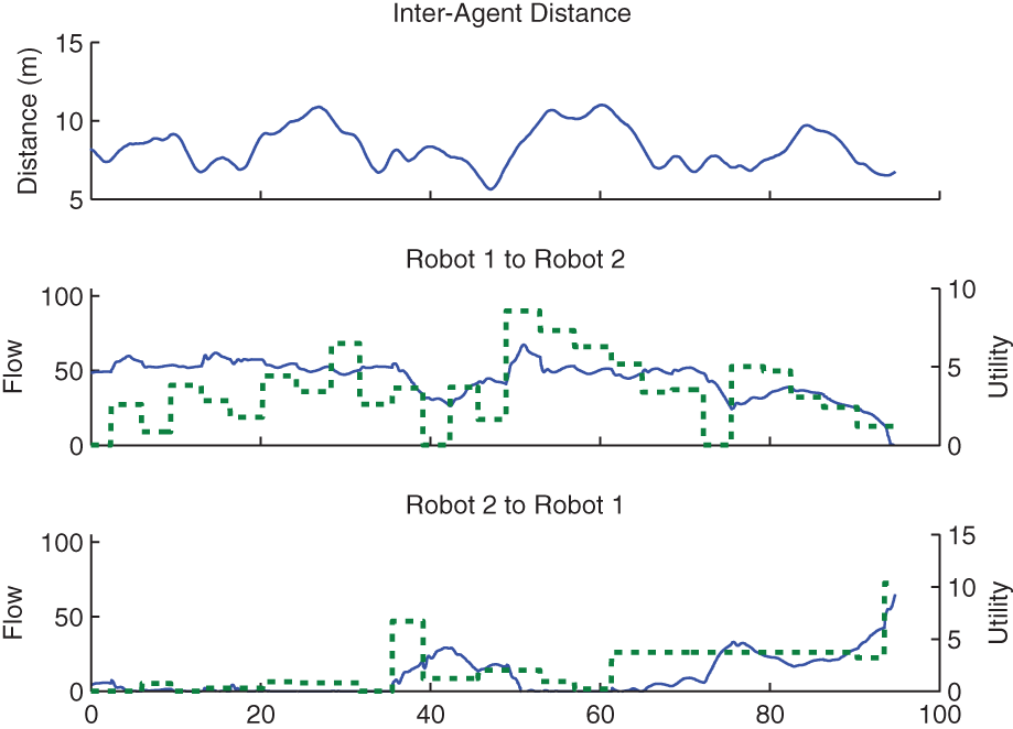
Inter-robot flow rates and sensor utility over time for the dynamic flow case of the two-robot experiment. In the first plot, the inter-robot distance is shown. In the lower plots, flow rate is shown as solid lines and sensor utility is shown as dotted lines. Flow rate varies with utility and available bandwidth varies with inter-robot distance.

OPEN IN VIEWER

Table 3

Average flow rates and Sensor Utility for the two-robot Experiment.

Link	Flow Rate	Sensor Utility
Robot 1 to Robot 2	44.80	3.42
Robot 2 to Robot 1	10.30	2.10

6.4. Three-sensor-node experiment

We also evaluated our approach in a more complex scenario. This scenario involves the two robots from the previous experiment with the addition of a stationary camera. The aim of this three-sensor-node scenario is to show the generality of our method and to emphasize the multicast behavior of dynamic information flow.

6.4.1. Experimental setup:

In this scenario, the two robots are aided in tracking by a Prosilica GC2450 camera acting as a bearing-only sensor. The camera is positioned outside the tracking region of interest opposite the robots. The camera sends raw images to Robot 2 which processes the images and shares the observations with Robot 1. Hence, wireless communication is required for three links: 1) the link from the camera to Robot 2, 2) the link from Robot 1 to Robot 2 and 3) the link from Robot 2 to Robot 1. In the experiment, the robots remained stationary. This does not affect the results of the demonstration since separation distance is ignored in this scenario. Simulation results with moving robots in a similar setup are shown later in Section 6.5.

The network diagram is shown in Figure 22. The experiment assumes that available bandwidth is sufficient for the two mobile robots to share observations. However, if images are received from the static camera then the wireless network becomes congested. The camera provides accurate tracking when the target is in its proximity and inside its field-of-view. Dynamic flow is expected to allow images to be sent from the camera in such a situation. The extra flow from the camera has to be accompanied by a simultaneous reduction of flow in the other links sharing the medium.

OPEN IN VIEWER

Fig. 22.

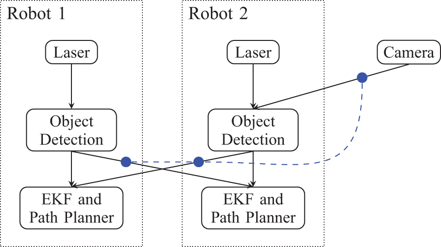
The threshold-DIF diagram for the three-sensor-node scenario. Virtual links are omitted for clarity.

All three communication methods were tested. In the unconstrained communication case, images from the camera were sent to Robot 2 for processing and caused congestion in the wireless network. The bandwidth limits on the wireless network effectively reduced the image transfer rate and consequently diminished the advantage of the unconstrained case.

6.4.2. Results:

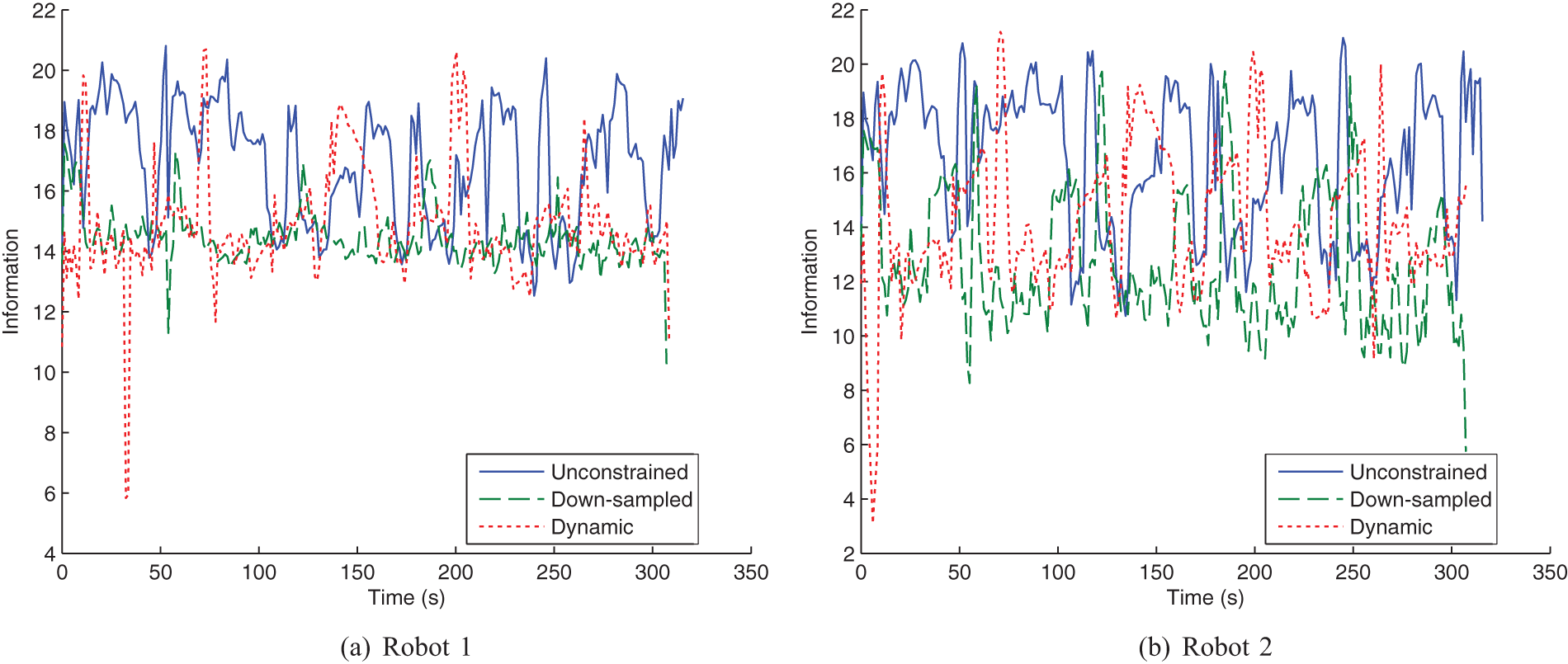
The information value for each of the robots’ estimates is plotted over time in Figure 24 with the corresponding average bars shown in Figure 25. The figures show that the dynamic case outperforms down-sampling for both robots. They also show better performance for the dynamic case in comparison to the unconstrained case for Robot 1, since the unconstrained case would have failed to produce the desired communication due to infrastructure bandwidth limitations. The results for Robot 2 show similar performance between the dynamic case and the unconstrained case.

OPEN IN VIEWER

Fig. 23.

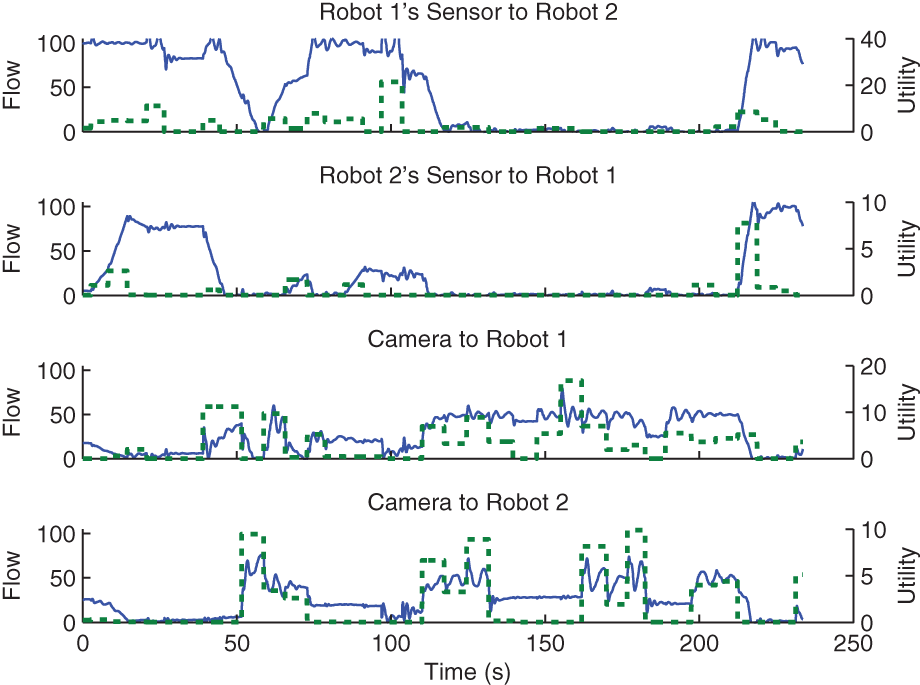
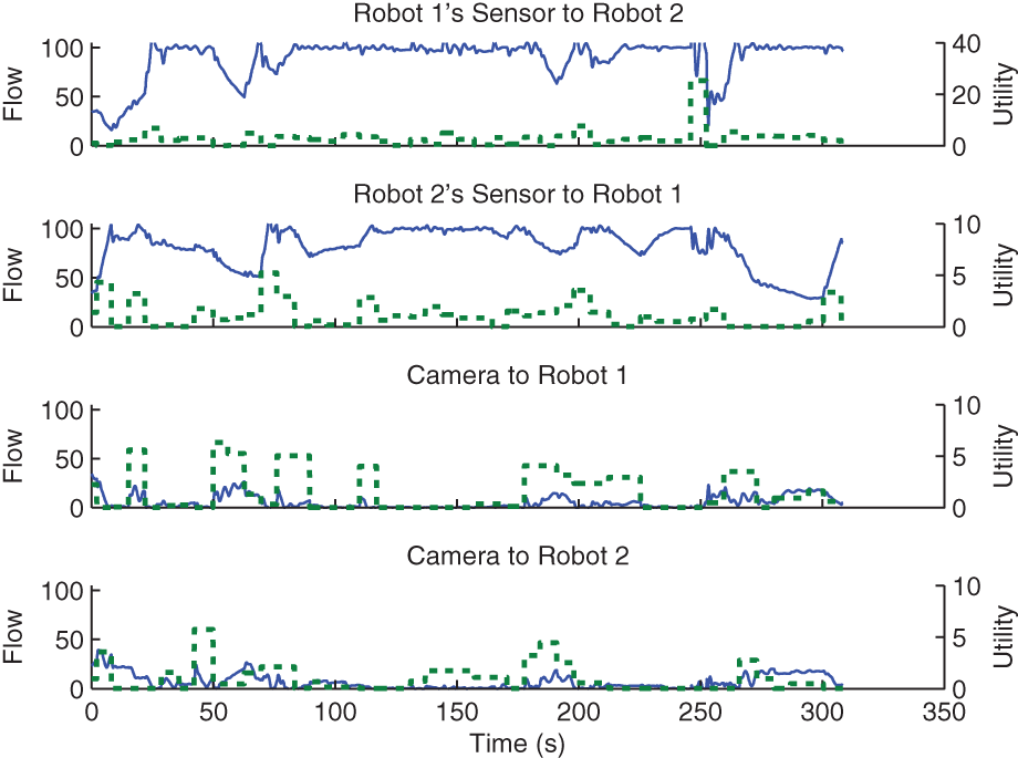
Inter-robot information flow and sensor utility over time for the dynamic flow case of the three-sensor-node experiment. Flow rates are shown in solid lines; sensor utility is shown in dashed lines. Based on the bandwidth constraints and the camera’s data rate, 50 is the maximum flow available for the data sourced from the camera. At approximately 120 s, communication from the camera interrupts communication between robots due to the increased utility of camera observations.

OPEN IN VIEWER

Fig. 24.

The information value (negative entropy) of the robots’ target estimate for the three-sensor-node experiment. Plots are shown for all three communication methods: unconstrained, down-sampled and dynamic.

OPEN IN VIEWER

Fig. 25.

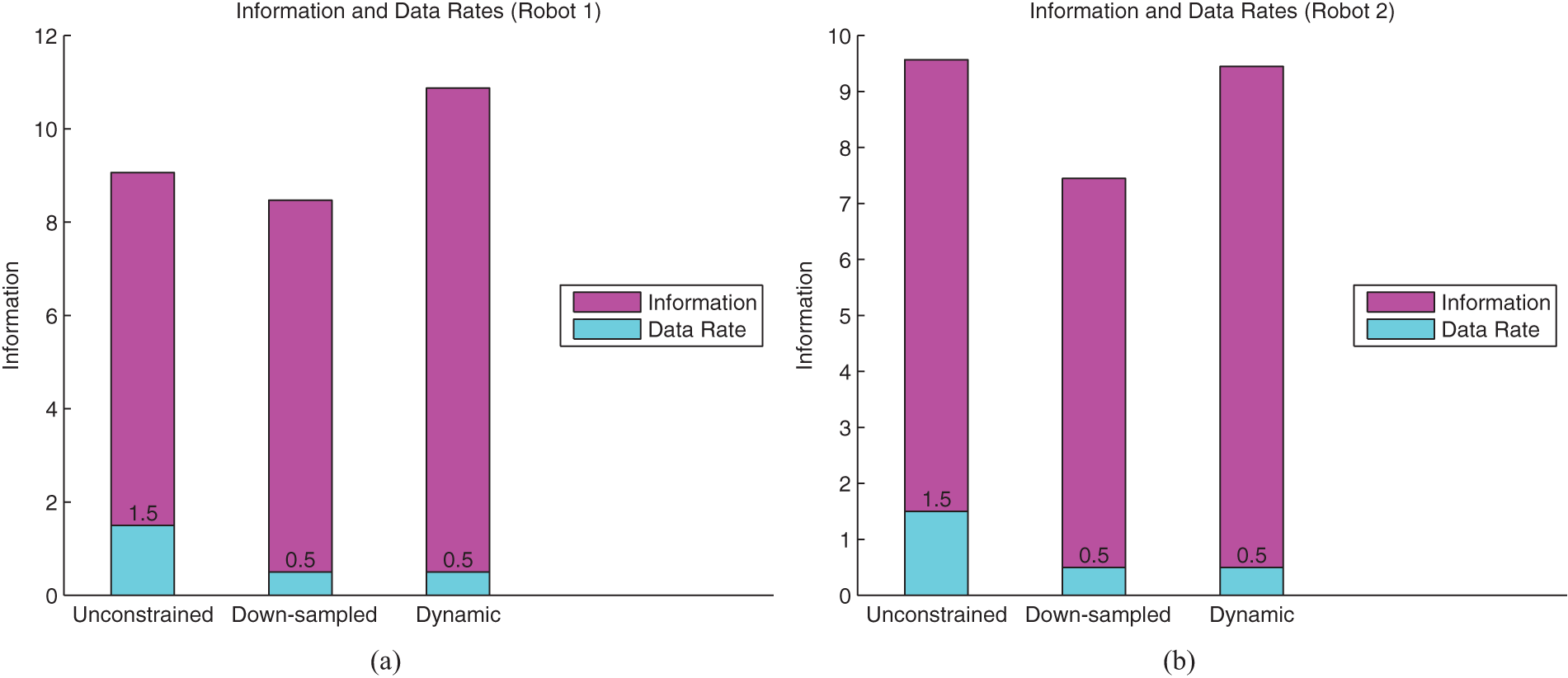
Time averages of the plots in Figure 24 shown in bar format. Data rates are shown superimposed. The dynamic information flow case has high average information gain performance with low average data rate.

One of the main objectives of this experiment is to highlight the multicast behavior. Multicast behavior can be observed by analyzing the bottom two plots of Figure 23. At times 80 s, 150 s and 190 s, the flow from the camera to Robot 2 retains a high value even though the camera utility for Robot 2 is low during those times. Robot 2 receives these observations without inducing additional cost since observations destined to Robot 1 are processed on-board Robot 2. Robot 1 receives these observations due to their high utility for Robot 1 but these observations must be processed on-board Robot 2 according to the system architecture. Multicast routing ensures that such flow does not get tallied twice. The top two plots confirm that the system obeys the bandwidth limits as the drop in flow takes place concurrently with the rise in flow from the camera. It should be noted that the maximum possible flow from the off-board stationary camera is only 50 units according to bandwidth bounds. The flow rate and sensor utility averages are shown in Table 4.

OPEN IN VIEWER

Table 4

Average flow rates and Sensor Utility for the three-sensor-node experiment.

Link	Flow Rate	Sensor Utility
Robot 1’s sensor to Robot 2	51.34	2.85
Robot 2’s sensor to Robot 1	24.68	0.50
Camera to Robot 1	26.29	3.40
Camera to Robot 2	24.89	1.88

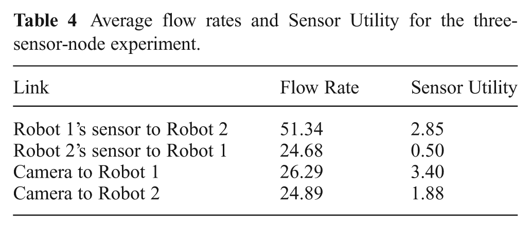
These results also validate the maximum flow approximation of total flow. The flow in each of the inter-robot links shown in the top two plots in Figure 23 holds data to only one destination. Therefore, there is no error arising from the maximum flow approximation for those links. The link from the camera holds data destined to both robots. At instances when the camera link is at zero or at maximum flow, there is no loss due to the maximum flow approximation. Also, the number of destinations in this case is two and hence the loss calculated from (19) is at most 25% of maximum flow for all other instances.

6.5. Three-sensor-node simulation

We repeated the experiment presented in Section 6.5 in simulation. Here, we allow robots to move in order to improve tracking performance.

6.5.2. Results:

The bottom two plots shown in Figure 26 highlight an aspect of multicast behavior different to that highlighted by the hardware analogue of this simulation. When only one robot evaluates a higher utility for camera observations, such as at times 120 s, 150 s and 220 s, no significant change in flow is observed. However, when both robots evaluate an improvement in the utility, the increase in the flow from the camera can be clearly seen.

OPEN IN VIEWER

Fig. 26.

Information flow and sensor utility for the three-sensor-node simulation. Flow rates and sensor utility are represented as in Figure 23. The maximum flow rate available for the data sourced from the camera is assumed to be 50. Flow rates vary with sensor utility.

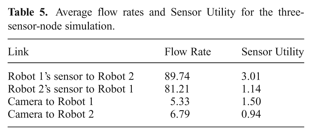
The information value of the robots’ target estimates over time is shown in Figure 27 with the corresponding average bars shown in Figure 28. As expected, unconstrained communication results in higher information on average. However, this communication setting violates the bandwidth bounds. Nevertheless, Figure 28 shows that the dynamic case outperforms the down-sampled case for both robots. Figure 27 shows that the dynamic case dominates the down-sampled case at time 70 s, between times 150 s and 200 s and between times 250 s and 300 s. Observations were received from the camera at these times for the dynamic flow case (as can be seen in Figure 26). These times correspond to the configuration where the target enters the camera’s field of view and becomes closer to the camera than the mobile robots. The flow rate and sensor utility averages are shown in Table 5.

OPEN IN VIEWER

Fig. 27.

The information value (negative entropy) of the robots’ target estimate for the three-sensor-node simulation. Plots are shown for all three communication methods: unconstrained, down-sampled and dynamic.

OPEN IN VIEWER

Fig. 28.

Time averages of the plots in Figure 27 shown in bar format. The data rates are shown superimposed. The improvement for Robot 2 achieved by dynamic communication over down-sampling using the same communication rates is clearly observed. The unconstrained method violates the bandwidth constraints and is only included as a benchmark.

OPEN IN VIEWER

Table 5.

Average flow rates and Sensor Utility for the three-sensor-node simulation.

Link	Flow Rate	Sensor Utility
Robot 1’s sensor to Robot 2	89.74	3.01
Robot 2’s sensor to Robot 1	81.21	1.14
Camera to Robot 1	5.33	1.50
Camera to Robot 2	6.79	0.94

Similar to the hardware case, we note there is no error arising from the maximum flow assumption in the links between the two robots. The loss occurring in the link from the camera is negligible.

6.6. Multiple-node simulation

We demonstrated our decentralized algorithm on a simulated 15-node threshold-DIF network. The purpose of the simulation is to demonstrate our approach for a problem that is not amenable to manually designed communication protocols.

The simulated network comprises five agents each equipped with a sensor, a processor and an estimator. The network has a fully connected topology such that each sensor is connected to all processors and each processor is connected to all estimators. The agents are spatially distributed evenly in a linear manner. Each sensor is assumed to produce data at a rate of 100 units. A global communication constraint of 500 units was applied. In addition, a per-link capacity constraint of 200 units was applied to each processor–estimator link. Sensor utilities were externally randomized and provided to the estimators.

Figure 29 displays, in chronological order, the routing state of the network at various time instances throughout the simulation. Each column represents one agent equipped with a sensor, processor and estimator. This configuration is a matter of choice rather than a restriction of the algorithm. The links shown in the figure represent those that carried more than 10 units of data during the simulation. The figure demonstrates the shift of flow from one part of the network to another as the sensor utilities change. More importantly, the routing states shown would be difficult to determine based merely on intuition.

OPEN IN VIEWER

Fig. 29.

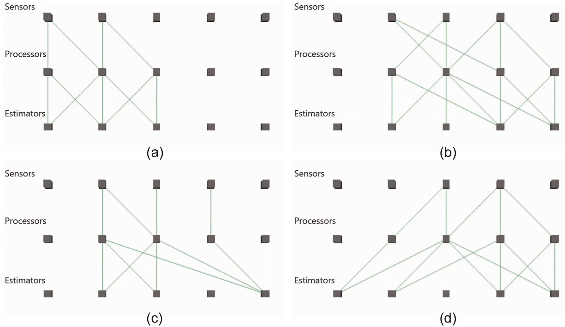
Routing state of multiple-node simulation at various times depicting active wireless links. Each column represents one agent equipped with a sensor, processor and estimator. Active links are represented by green lines. A link is considered active if it holds more than 10 units of data flow.

6.7. Monte Carlo simulation

To validate the performance of dynamic information in comparison to down-sampling, we conducted a Monte Carlo simulation for the experimental setting of Section 6.3. The aim of the simulation is to analyze the statistical significance of performance improvement due to our solution to threshold-cost-DIF.

The results of the Monte Carlo simulation are shown in Figure 30 in box-plot format. For each communication method, we ran 20 randomly initialized trials running for 1 min each. The results shown assume each trial as one sample. Dynamic communication outperforms down-sampling with p-value of less than 0.03 based on Welch’s t-test.

OPEN IN VIEWER

Fig. 30.

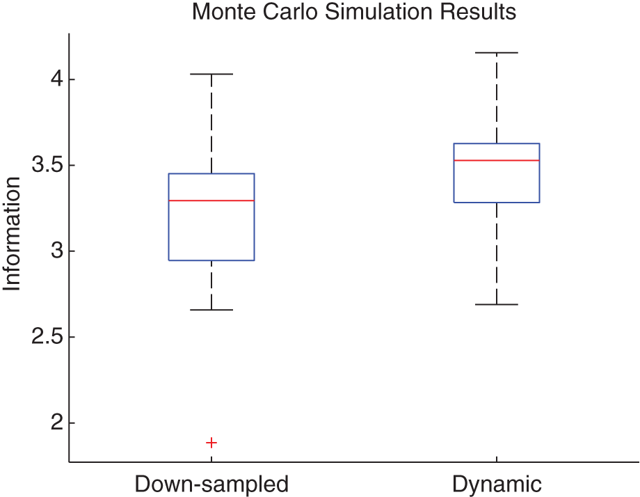
Monte Carlo simulation results comparing down-sampling with dynamic information flow. Each method was tested on the two-robot scenario for 20 trials running for 1 min each. In the results depicted, a trial acts as one sample. The box extents represent the first and third quartiles, while the whiskers represent the extrema. The median is represented by the horizontal line inside the box.