
Abstract
This paper investigates the problem of confirming the identity of a candidate object (expected to be a target based on some crude visual clues) with a mobile robot equipped with visual sensing capabilities. We present a method whose main novelty is to mix localization of the robot relative to the candidate object and to confirm that it is the sought target. This twofold approach drastically reduces false positives. Identity confirmation with this twofold goal is modeled as a Partially-Observable Markov Decision Process, where the states are the cells of the space decomposition. It is solved using Stochastic Dynamic Programming with imperfect state information. A robotic system using this method has been implemented and tests have been carried out both in simulation and with a real robot. The experiments empirically validate the use of various metrics, and demonstrate their ability to perform well in different settings.
1. Introduction
In this paper we investigate the problem of confirming the identity of an object using a mobile robot equipped with a camera, a range sensor (to avoid collisions), and a vision software module referred to as the target detector (or, more simply, the detector). More precisely, we will describe a method to perform the third step of the following scenario;
The robot is instructed to find a certain object T, hereafter called the target, in its environment.
Using a space coverage method (e.g. the method described in Espinoza et al. (2011)), the robot detects an object C, called the candidate, which looks like T based on some crude (but easy to detect) visual clues, such as color, texture, or general shape.
The robot moves on a horizontal floor around C to achieve suitable viewpoints, allowing the target detector to eventually confirm (or infirm) that C is actually T.
The main novelty of our method is that it mixes localization of the robot relative to the candidate object C and confirms that C is the target T. This twofold approach drastically reduces false positives. The robot is given a probabilistic observation model of the response of the target detector, trained over a cell decomposition of the space surrounding T (Section 3). During the confirmation process, the robot never knows its exact position; instead, the robot’s belief about its position is also modeled by a probability distribution over this cell decomposition (Section 4). By performing successive moves (Section 5), the robot acquires several images of C from different viewpoints and runs the target detector on each image. After each move it uses the observation model to update its position belief. The robot’s goal is twofold (Section 4). One part of the goal is to compute a motion strategy that will eventually reach a position P, where the target detector confirms with high confidence that C is actually T. But this goal alone would be prone to produce false positives, especially if other objects look very similar to T from some viewpoints. The other part of the goal is to compute the motion strategy so that the robot expects with high probability that, upon reaching P, the detector will confirm with high confidence that C is actually T. This twofold goal drastically reduces the risk that the detector incorrectly confirms that C is T. The identity confirmation process is modeled as a Partially-Observable Markov Decision Process (POMDP) (Candido and Hutchinson, 2011; Kaelbling et al., 1998) where states are the cells of the space decomposition. Motion policies are computed using Stochastic Dynamic Programming with imperfect state information (Bertsekas, 2000).
The ability of a mobile robot to reliably confirm the presence of a target object in an environment has a wide range of potential applications, especially as an end-module for search problems, as suggested in the above scenario. There has already been a substantial amount of research studying how a robot or a team of robots should search an environment to find a static object or a moving agent (adversarial or not) (Chung at al., 2011; Guibas et al., 1999; Tovar and LaValle, 2008). In this research the target is usually considered found when a robot has established a line of sight with it. However, this condition requires the robot’s detector to reliably identify the target from any viewpoint at any distance. Some research attempts to fulfill this condition by creating powerful detectors (Felzenzwalb et al., 2008; Grauman and Darrel, 2005; Lowe, 2004). Instead, we consider here that a detector will always be imperfect and that the ability of the robot to move around an object and take images from different viewpoints should be exploited to overcome the limitations of the detector. This combination is particularly suitable when the target differs from other objects by few small distinctive features visible only from limited viewpoints, or when elements of the environment (e.g. poor illumination and textured background) may deceive the detector. For instance, to reliably identify your luggage on a conveyor belt at an airport, you look at it from different viewpoints in order to detect special features that differentiate it from similar luggage, for which you had no prior models, and you do not remain static. So, the problem considered here is a target confirmation problem, which differs significantly from traditional object recognition problems, as only the observation model of the target is available. Confirming that an object is a given target and not another, possibly similar, object of an unknown model, is a challenging problem.
A robotic system has been implemented using our method, and tests have been carried out both in simulation and with a real robot. Our simulation experiments were intended to test our approach under well-controlled conditions. We created a textured virtual environment, and the detector was applied to synthetic images generated from the successive robot’s viewpoints. In this paper we report on four experiments in simulation (Section 7). Some of our goals were: to verify that our system is able to discriminate between similar objects and is not confused by targets with similar appearances from different viewpoints, and to analyze its behavior when localization errors increase. We then present five experiments with a real robot, a Pioneer P3-DX (differential-drive robot) equipped with a USB camera and a Sick-LMS200 range sensor, aimed at further assessing our approach (Section 8). In these experiments, we vary two sets of parameters. Parameters in one set are related to the planner, e.g. planning horizon, number of cells in space decomposition. Parameters in the other set are related to the environment and the target detector: illumination of the environment, environment background, textures, sizes and colors of the targets and the size of the training set of images. Overall, the experiments empirically validate our method, evaluate its performance along various metrics (success rate, planning time, number of sensing operations, length of robot path), and demonstrate its ability to perform well in a broad variety of settings, even with an imperfect detector. They also reveal interesting insights and suggest topics for additional future research.
A preliminary version of a portion of this paper appeared in Becerra et al. (2014). The main differences are the following;
We no longer assume that the robot knows the position of the center of the candidate object. Instead, only the direction of the object center is now needed, and this is estimated using the data provided by the range sensor. Moreover, a new experiment in simulation shows that our system tolerates large errors in the estimated direction.
The preliminary version did not include experiments with a real robot. Here, we present and discuss five such experiments. They test in particular the impact of variations in scene illumination and in the number of cells of the space decomposition.
A new experiment in simulation which considers the presence of obstacles around the candidate object. These obstacles create both motion and visibility constraints.
The main contributions of our work are threefold: (1) to reduce false positives, our method mixes localization of the robot relative to the candidate object C and confirmation that C is the target T; (2) our experiments show that if an observation model contains too much uncertainty then planning too far ahead may have a negative effect on the effectiveness of the confirmation process; (3) experiments demonstrate that our method correctly handles candidate objects that are distinct from but similar-looking to targets, and that it tolerates poor illumination conditions, targets with no neat features and obstacles that produces both motion and visibility constraints.
Section 2 discusses related work. Section 3 describes the target detector and the observation model of a target. Section 4 formulates the mixed identification/localization process as a POMDP. Section 5 defines the motion commands available to the robot and the corresponding transition model of the POMDP. Section 6 describes the use of Stochastic Dynamic Programming to compute motion policies. Section 7 presents and discusses four experiments carried out in simulation. Section 8 reports on five experiments executed with the real robot. Section 9 concludes the paper and suggests directions for future research. Appendix B provides details on how transition probabilities of the POMDP are computed. Appendix C describes the implemented robotic system and the software modules running on it.
2. Related work
Several variants of search and pursuit-evasion problems have attracted considerable interest in the robotics community (Chung at al., 2011; Guibas et al., 1999; Isler at al., 2005; Lee et al., 2002; Park et al., 2011; Sarmiento et al., 2003; Tovar and LaValle, 2008). Particularly interesting is the problem of finding a target in an environment of given geometry using the fewest number of robot searchers. For instance, in Guibas et al. (1999) the searchers, which are equipped with visibility sensors, are required to plan and perform coordinated trajectories that guarantee the eventual visual detection of a mobile target (also called the evader), even if it tries to escape the searchers. However, a common strong assumption in this type of work is to represent both the searchers and the target as points and to consider that the target is detected as soon as the line segment between a searcher and the target intersects no obstacle, i.e. a line of sight exists between them. As mentioned in Section 1, this kind of work would benefit from using a more realistic target detector.
The problem of searching static objects in an environment has also been treated as an active vision problem (Tsotsos and Shubina, 2007; Ye and Tsotsos, 1999) by selecting several successive viewpoints. In fact, active vision (Aloimonos et al., 1988; Bajcsy, 1988) - the use of motion to acquire pertinent sensing information about an environment - is a recurrent theme in robotics. It arises in many applications, for instance, in robotic manipulation (Jang et al., 2008; Motai and Kosaka, 2008), surveillance (Bakhtari et al., 2009; Schroeter et al., 2009), tracking (Barreto et el., 2010), object modeling (Pito, 1999), localization and mapping (Fintrop and Jensfelt, 2008; Kaess and Dellaert, 2010; Zingaretti and Frontoni, 2006), and object recognition (see below), to name but a few. A rich survey of active vision methods used in robotic systems is given in Chen et al. (2011). The active vision approach that we propose in this paper mixes localization and identification. Unlike in Fintrop and Jensfelt (2008), Kaess and Dellaert (2010) and Zingaretti and Frontoni (2006), localization is not the main goal. It is only used as a source of information in order to better plan the next viewpoints, and ultimately to confirm the identity of an object with greater reliability.
The goal of object recognition is usually to detect and identify important objects and in some cases to estimate their poses. Some of the earliest work on this subject is presented in Bajcsy (1988) and Krotkov and Bajcsy (1993). This line of research can be organized according to different criteria, e.g. whether the sensing device is static (Lowe, 2004) or not (Browatzki et al., 2012), whether view planning optimizes only over the next viewpoint (Browatzki et al., 2012; Eidenberg and Scharinger, 2010; Meger et al., 2010) or over a sequence of viewpoints (Atanasov et al., 2014), and which optimization function is used for view planning. Regarding optimization, a common approach is to use an entropy-related information gain criterion (Eidenberg and Scharinger, 2010; Laporte and Arbel, 2006; Meger et al., 2010; Pito, 1999). A different type of optimization criterion quantifies a tradeoff between the length of the sensor movement, the energy expenditure to move the sensor, and the expected cost of an incorrect classification (Atanasov et al., 2014). Here we propose yet another type of optimization criterion aimed at guiding the robot toward a position where, with high probability, the target detector will confirm with high confidence that the candidate object is actually the target. Moreover, unlike some recognition methods (e.g. Atanasov et al. (2014)) that require an accurate estimate of the sensor pose to plan the next best views, our approach models the position of the robot (and its sensors) relative to the candidate object as a probabilistic distribution over a cell decomposition of the space around the object.
Also relevant to our work, a method for learning viewpoint detection models for object categories is presented in Meger et al. (2010). The generated models are used in a sequential object category recognition task, where the robot must infer the likelihood that an object has a category label x given N detector responses received so far. Each new viewpoint is chosen to minimize the entropy over the posterior belief of the category labels of the object. Our approach is also based on the idea that the choice of viewpoints is critical to identify an object. However, our formulation of the identification problem as a POMDP does not lead to concentrating the peak of a probability distribution over a collection of object categories on a particular category, as is done in Eidenberg and Scharinger (2010) and Meger et al. (2010). Instead, it is focused on one single object, the target, and only considers the model of this object; thus it does not need models for many objects that are not potential targets.
As we mentioned in the Introduction, the problem of sweeping an environment to find a target object has been addressed in Espinoza et al. (2011). The work presented in this paper is complementary to this previous work. We think that, to be performed quickly, the detection of a target during an environment sweep must only rely on crude, but easy-to-detect, visual clues; hence it cannot be fully reliable. Therefore, once a candidate object has been detected, a different approach is needed to confirm (or infirm) that this object is actually the target. The remainder of this paper presents such an approach.
3. Target detector and observation model
We assume that during the confirmation process, the candidate object C is static and not significantly hidden by obstacles, and that the robot moves on a planar horizontal surface around C. We define the position of the robot to be that of the camera mounted on it. Either the robot can rotate in place (e.g. a differential-drive robot), or there is a revolute joint (around a vertical axis) between the robot and the camera, so that pointing the camera toward C does not introduce additional constraints to the path followed by the robot.
Before the robot can be used to confirm that a candidate object C is a certain target T, it must be equipped with a vision software module
In our implemented system, the detection method used in
The robot should be equipped with different detectors
The observation model of T is a trained probabilistic model of the response of
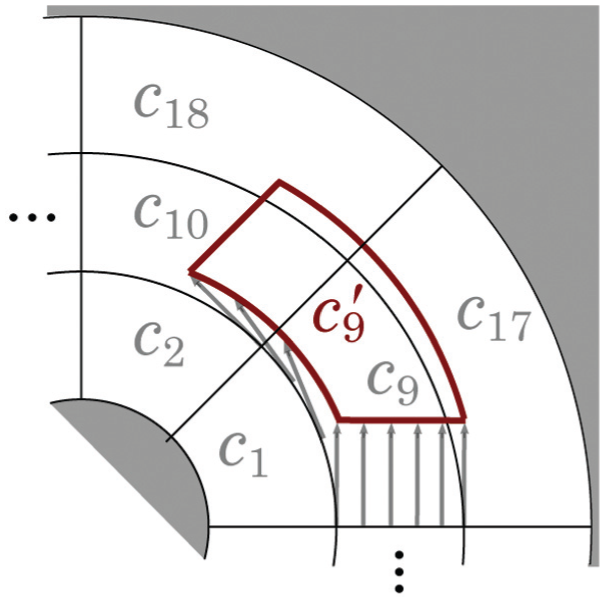
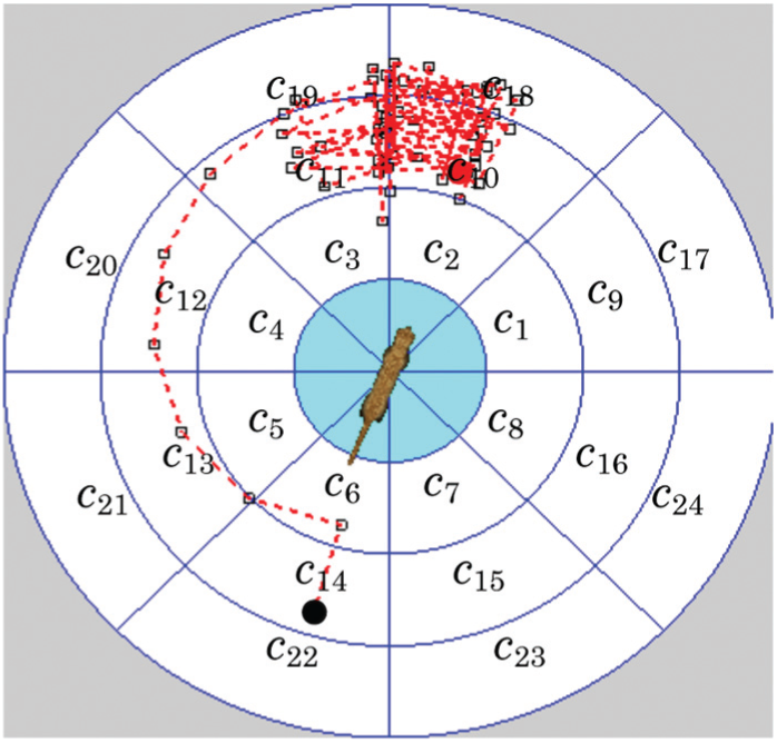
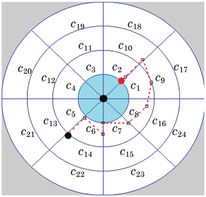
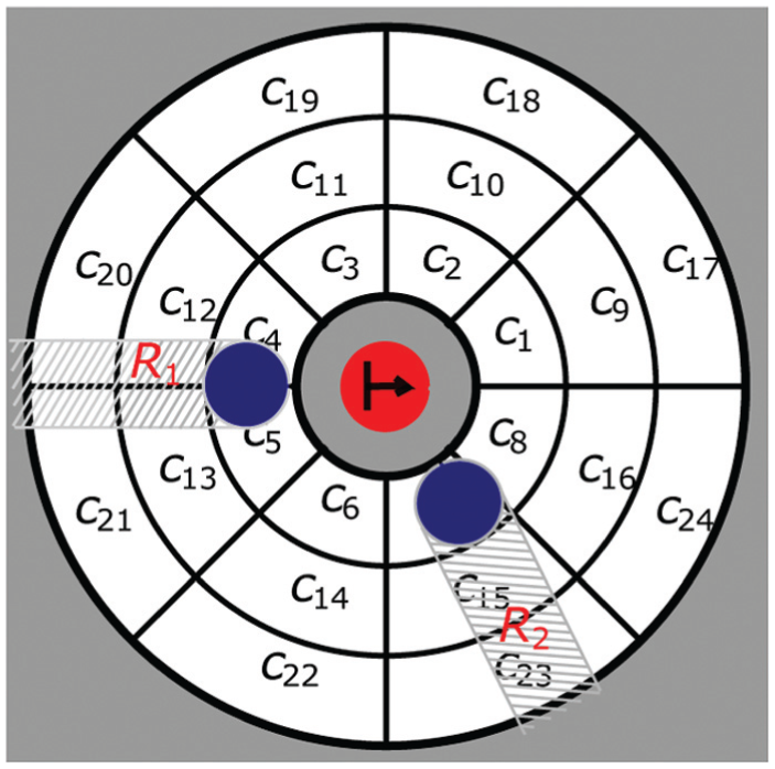
Figure 1 shows a particular decomposition made of
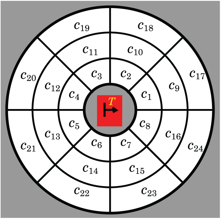
Cell decomposition of the space around T.
Given
4. Confirmation process and robot localization
Consider now the situation reached by Step 2 of the scenario presented at the beginning of Section 1: based on simple visual clues the robot has detected an object C that may be the target T, but it is not sure yet that C is T. The confirmation process (Step 3 of the scenario) consists of computing and executing a series of motion commands
We assume around C the existence of the same cell decomposition
At each time t, the robot’s belief about its position relative to the potential target is modeled at the cell resolution of X by a probability distribution
The visual sensors of the robot in our implemented system include a range sensor (see Section 8.1) that is used at Step 2 of the scenario, in order to bring the robot within a distance of C that is compatible with the inner and outer radii of the decomposition (for instance at a distance roughly equal to the outer radius minus the inner one). The robot knows nothing else about its initial position. So, at time
At every time
where
To confirm that C is the target T the robot must reach a position at some time

where
As formulated above, target confirmation is a Partially-Observable Markov Decision Process (POMDP) (Candido and Hutchinson, 2011; Kaelbling et al., 1998), where X is the set of states,
5. Motion commands and transition model
To complete the formulation of the POMDP introduced above, we now present the state transition model, that is, the set of motion commands that the robot can perform and the probability distribution
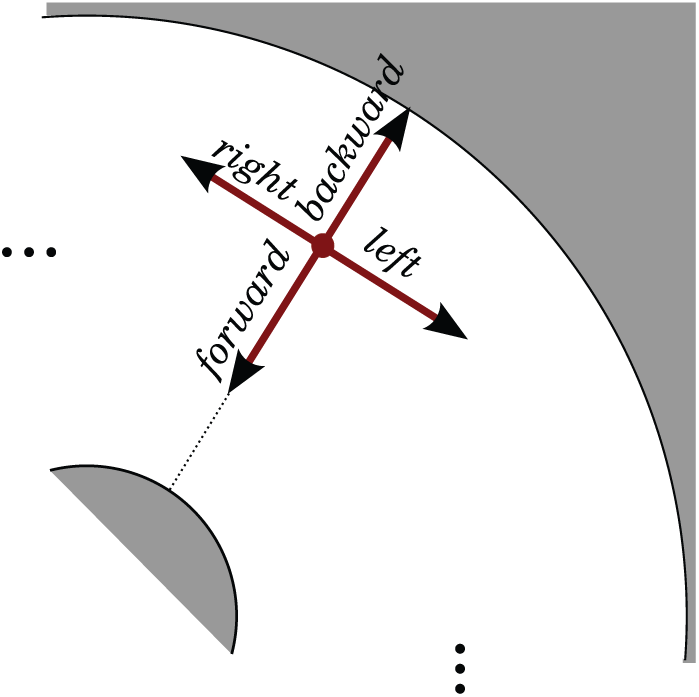
At each step t of the confirmation process, we allow the robot to choose among four motion commands

defined as follows and illustrated in Figure 2.
The command forward makes the robot move in the direction of the estimated center of C in the image taken at t. The command backward makes the robot move in the opposite direction.
The commands left and right make the robot move perpendicular to the estimated direction of the center of C at time t, in the clockwise and counter-clockwise directions respectively.
Motion commands.
In our implemented system the length of each motion is set to be slightly greater than the distance between two consecutive circles of the decomposition. This choice ensures that the robot crosses cell boundaries often, and thus gets a variety of viewpoints over a few moves. However, for the commands forward and backward, the robot uses its range sensor to remain within a distance of C compatible with the inner and outer radii of the decomposition X: if it gets too close to C or too far from it, then the length of the motion is reduced.
Recall from Section 4 that the robot estimates its position at the cell resolution in X. This means that when the robot believes that its position is within a cell
Consider an arbitrary point p in
If
If
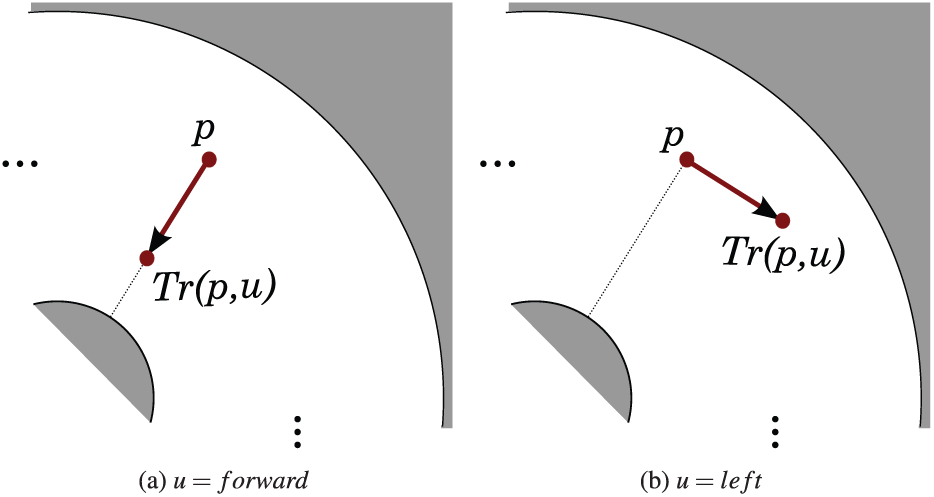
Transform
We define
The probability
This calculation makes the implicit assumption that the robot moves are “ideally” performed toward and away from the center of X (for forward and backward) and around this center (for left and right). However, the robot never tries to localize the decomposition X relative to C, as it does not even know whether the object C is actually the target T. Nevertheless, we believe that when C is T, the moves performed by the robot are close to these ideal moves. The experiments with a real robot (Section 8) validate this claim. Moreover, Experiment #4 in simulation (Section 7.5), which analyzes the impact of increasing errors in the estimate of the direction of the center of X, demonstrates that our method tolerates large errors quite well, as long as the candidate object remains within the field of view of the camera. In the future, if needed, the uncertainty in the direction of the center of X could be taken into account in the computation of the probability
The transition probabilities
6. Computation of a motion strategy
In Section 4, we have formulated the process of confirming the identity of C as a POMDP in which the states are the cells of X. Here, we compute a motion strategy by using Stochastic Dynamic Programming (SDP) with imperfect state information as proposed in Bertsekas (2000).
We specify two horizons: a planning horizonN and an execution horizon
The SDP-based planner computes a motion strategy in the form of a policy
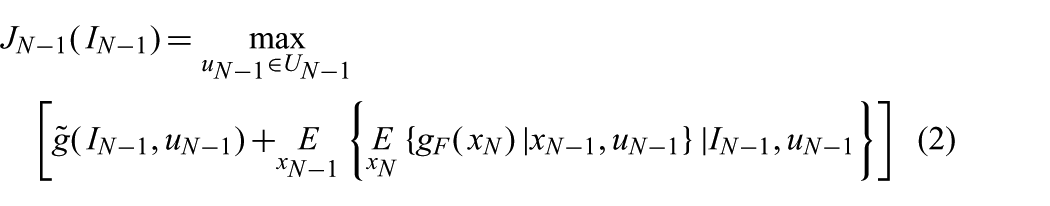
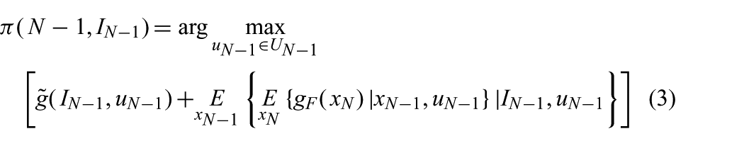
and for
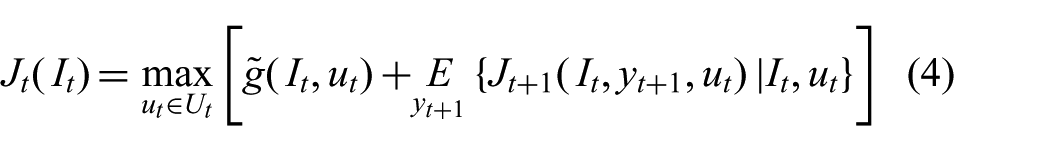
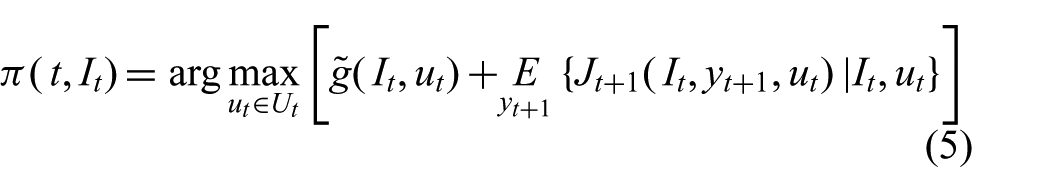
Since we want the robot to reach a position where the condition
In Experiments #1 and #2, reported later in this paper, the other gain function
Every plan generated by the SDP-based planner is immediately executed. If the confirmation condition is achieved, i.e. if the robot reaches at time t a position where the condition
There are clearly tradeoffs in setting the values of N and
7. Experiments with a simulation robot
7.1. General setting
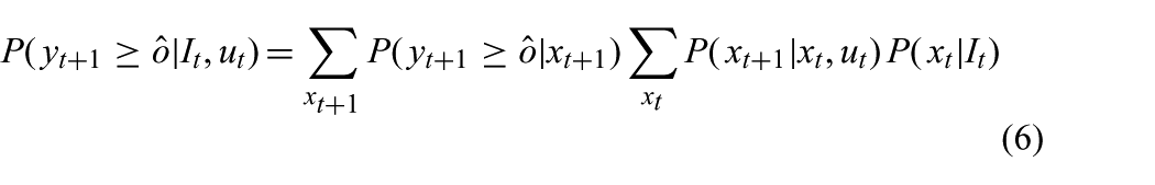
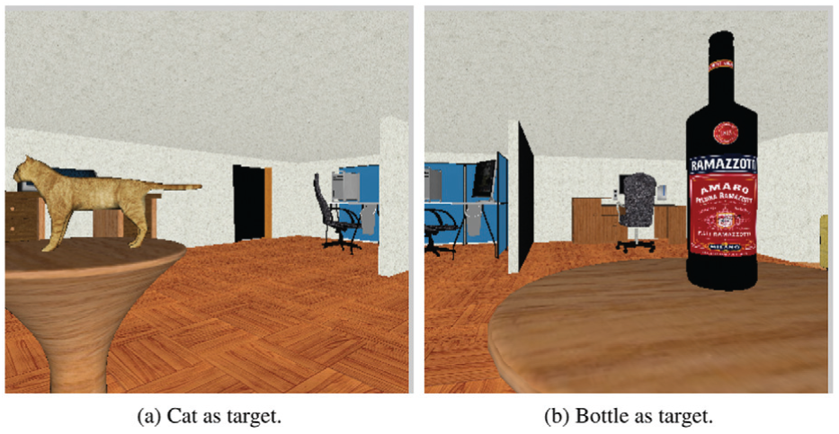
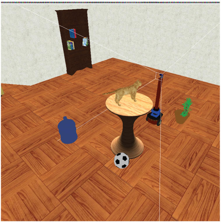
We created the textured virtual environment shown in Figure 5 in order to perform basic tests of our approach under well-controlled conditions. The object to be identified is placed at the center of the circular Table in the middle of the room. The simulated robot can move around this Table. Synthetic images from the viewpoint of a virtual camera mounted on the robot are generated at successive positions of the robot, and the detector
Virtual environment.
For each target T, the detector
In all the experiments reported in this section the planner uses the 24-cell decomposition shown in Figure 1 (we will vary the number of cells in Section 8.5). For each target T, the detector
In all experiments the center of the cell decomposition X is the center of the circular table. In Experiments #1, #2, and #3, the robot knows exactly the position of the table’s center, and therefore performs the four motion commands with accurate knowledge of the direction of this center. In Experiment #4, we will consider the case where this knowledge is imperfect, and we will analyze the impact of increasing errors in the estimate of the direction of the center. In Experiments #1 and #2 the gain function
In all the statistics tables shown below, the average numbers of sensing locations, path lengths and planning times are computed only over the runs that achieve confirmation.
7.2. Experiment #1: Plastic cat
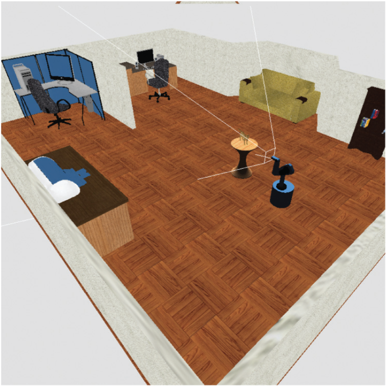
The purpose of this experiment is to verify the ability of our method to reliably identify an object, and to compare its performance with other motion strategies. The target is the plastic cat shown in Figure 6a. The placement of the cat on the table and the cell decomposition used for training the detector are shown in Figure 6b. We chose cell
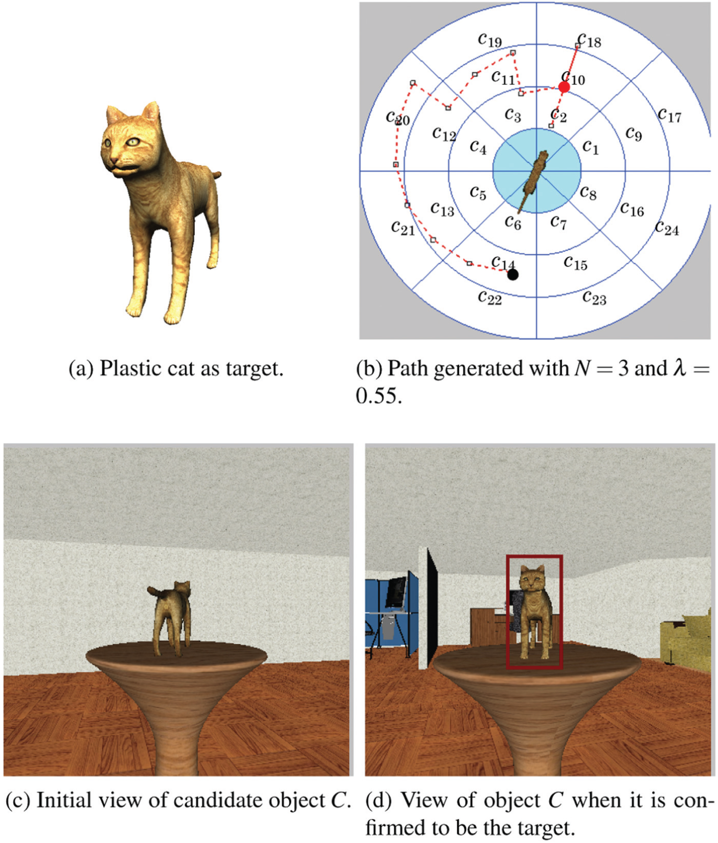
Illustrations for Experiment #1.
Observation model
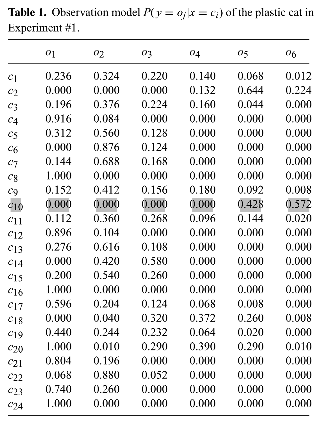
To test our method, we placed the robot in cell
Note that the combination of equation (6)and the observation model of Table 1 determines the upper-bound
The path followed by the robot in a run with
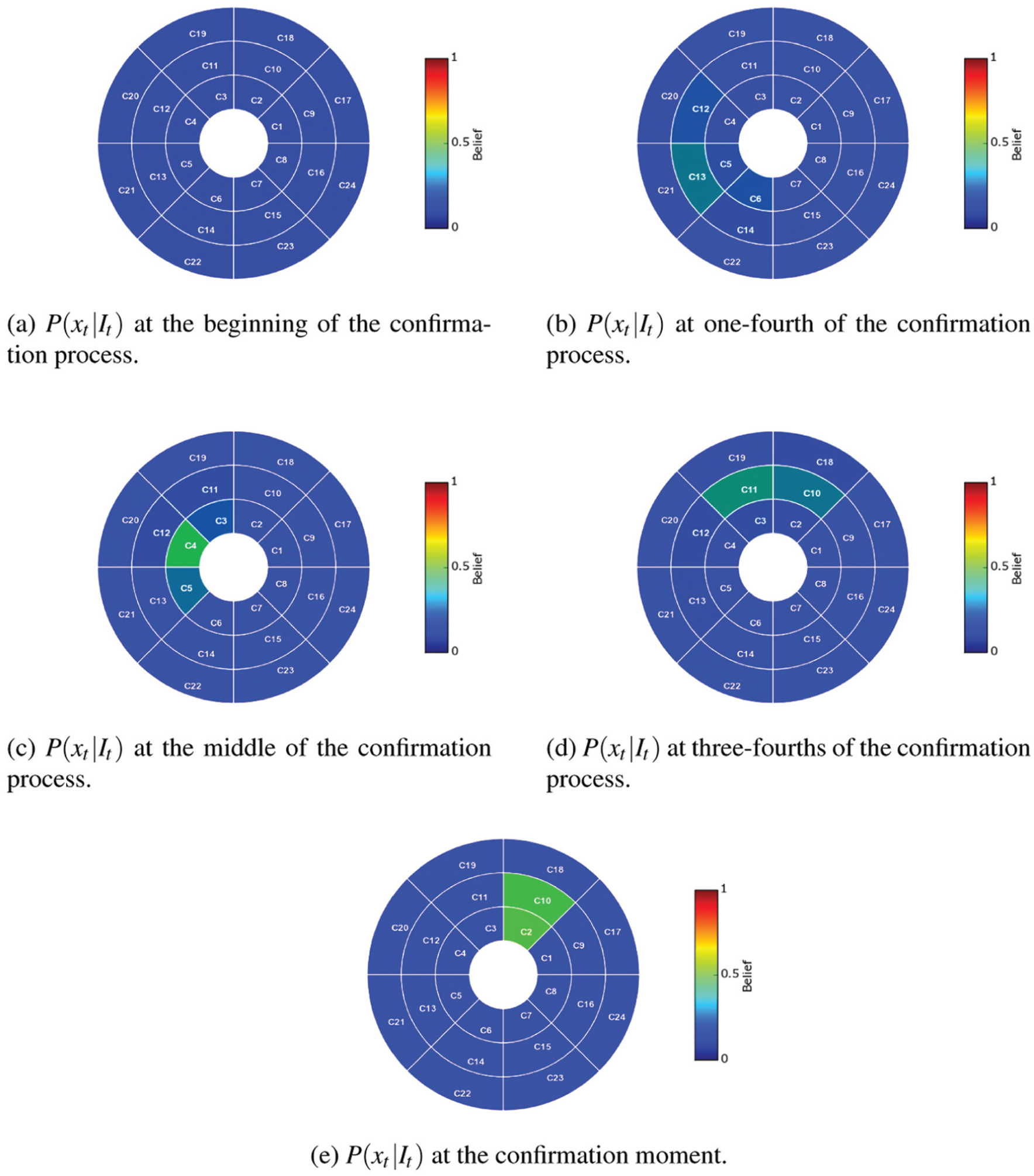
Evolution of probability distribution
For comparison, we also ran separately two different motion strategies. One is a “fixed strategy”, in which the robot moves around the candidate object in clockwise direction. The other is a “random strategy” in which the robot performs one of the 4 motion commands picked uniformly at random at each step. For both strategies, the maximum number of steps was set to
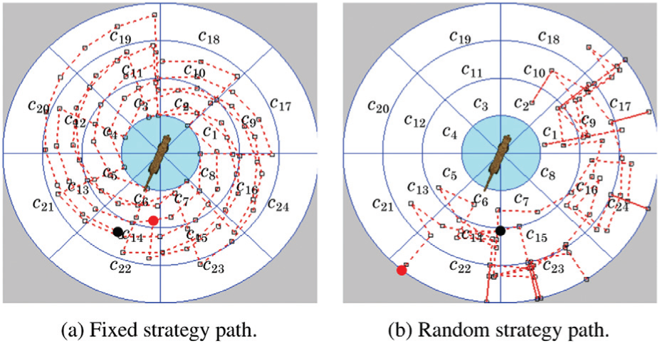
Two sample paths using fixed and random strategies with
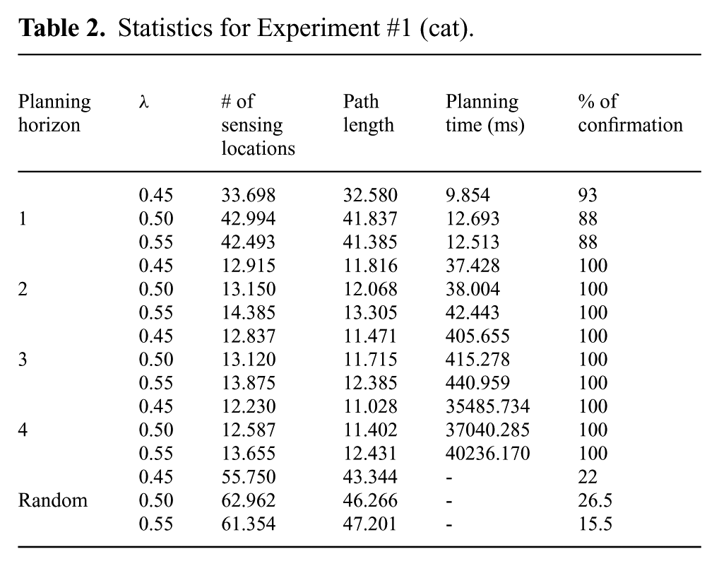
Table 2 shows some statistics (average number of sensing locations, average path length, and average total planning time) for Experiment #1, as well as the percentage of successful confirmations. Each line of the table was obtained over 200 runs with different initial positions of the robot within cell
Statistics for Experiment #1 (cat).
Path generated with
In this experiment our method produces smaller numbers of sensing locations and shorter path lengths when the planning horizon N increases. However, planning time also increases quickly with N (and also with
7.3. Experiment #2: Two similar bottles
The purpose of this experiment is to verify that our robot is able to discriminate between similar objects. We have two bottles, the “true” bottle shown in Figure 10a and the “false” bottle shown in Figure 10b. The true bottle has a circular label that the false bottle does not have. Apart from this label, the two bottles are identical. The target is the true bottle.
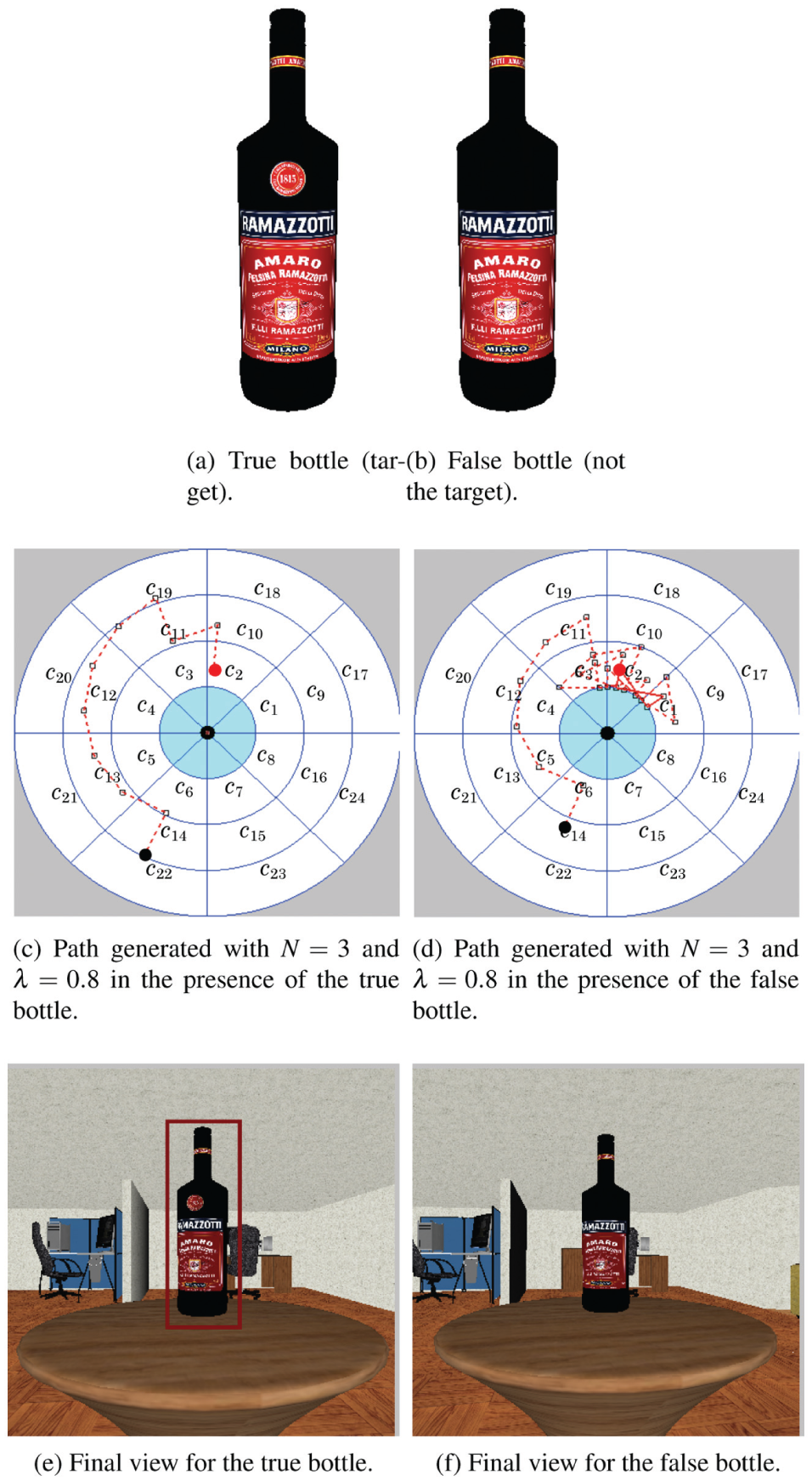
Illustrations for Experiment #2.
Like in Experiment #1, cell
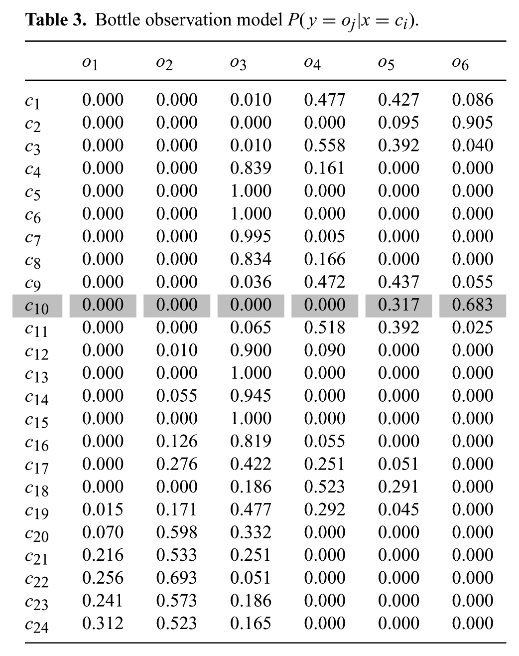
Bottle observation model
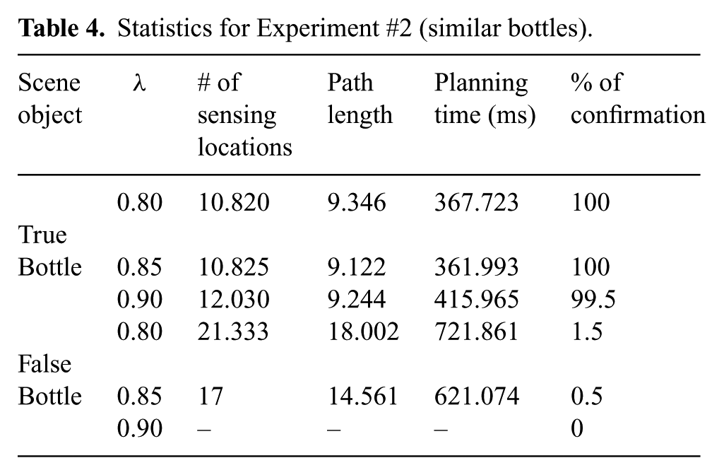
We tested the ability of our method to confirm (or infirm) the identity of each of the two bottles by placing them at the center of the table with their labels oriented as during the training of the detector. For each bottle we performed runs with a planning horizon N set to 3 and an execution horizon
Statistics for Experiment #2 (similar bottles).
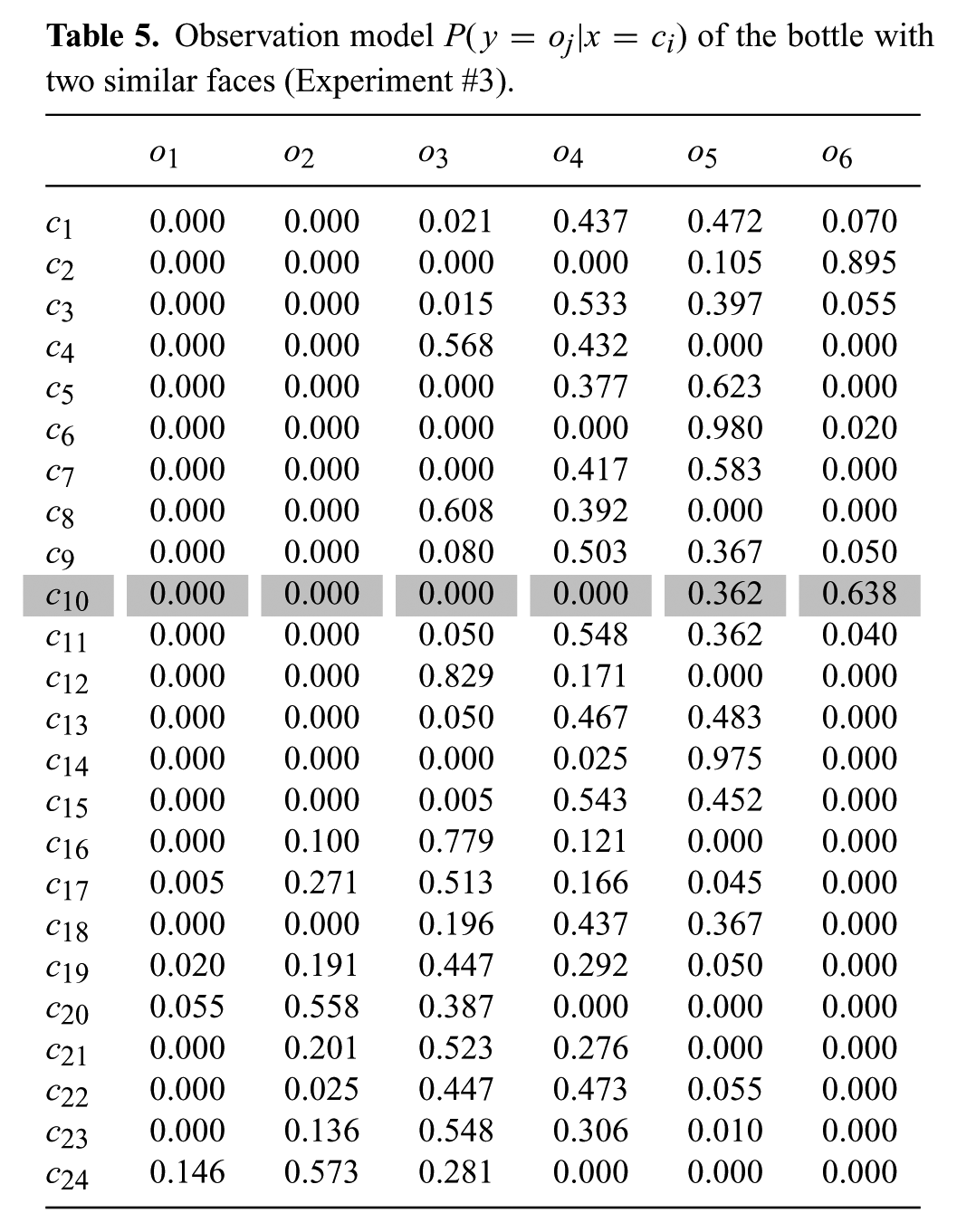
7.4. Experiment #3: A bottle with two similar faces
Here our goal was to observe the behavior of our method when the target has similar appearances from two different viewpoints. The target is a bottle that looks as in Figure 10a on one side and as in Figure 10b on the opposite side. The detector is trained in cell
Observation model
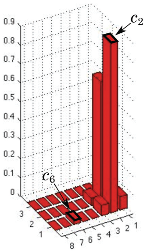
For both
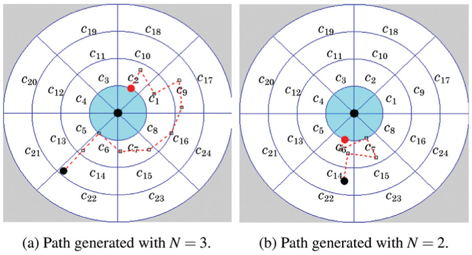
Sample paths for bottle with similar appearances from different viewpoints.
When
To address this local-maxima issue when small planning horizons are used, we added another gain function
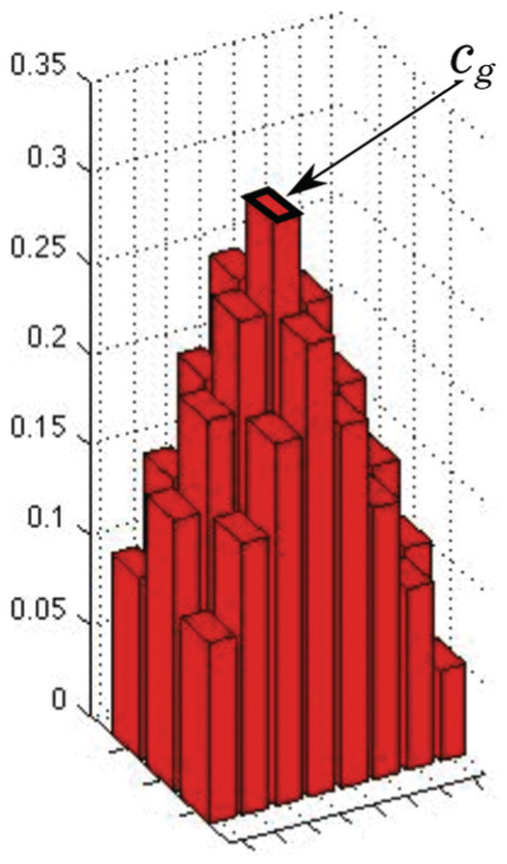
Function
Robot path with
In all the experiments reported in the rest of this paper (both in simulation and with a real robot) equations (2) and (3) include the additional gain function
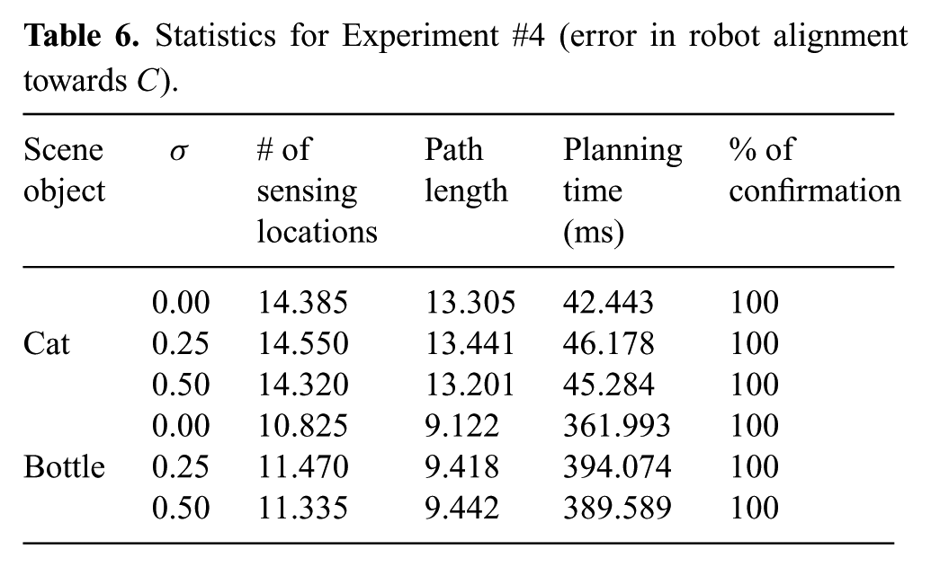
7.5. Experiment #4: Imperfect knowledge of the table’s center
To perform the four motion commands, the robot must estimate the direction of the center of the cell decomposition X. In our setup, this center coincides with the center of the circular table. In Experiments #1, #2, and #3, the robot knew exactly the position of the table’s center and therefore performed the four motion commands with accurate knowledge of the direction of X’s center. We now consider the case where this knowledge is imperfect and we analyze the impact of increasing errors in the estimate of the center’s direction (from now on referred to as orientation errors).
We perform runs with two successive targets: first the cat of Experiment #1, next the true bottle of Experiment #2. We test the impact of orientation errors with different planning horizons by setting N to 2 when the cat is the target and to 3 when the bottle is the target. To create an orientation error, we shift the actual direction of the table’s center by an angle picked according to a mean-zero normal distribution truncated between
Robot views of the cat and bottle with orientation errors.
The quantitative results are summarized in Table 6. The most important result is that the two targets were confirmed in all runs for every value of
Statistics for Experiment #4 (error in robot alignment towards C).
7.6. Dealing with obstacles generating motion and visibility constraints
In this subsection we present an extension of our method to deal with obstacles that create both motion constraints and visibility occlusions. Since a crude visual method has detected the candidate object, this object is visible at the beginning of the confirmation process.
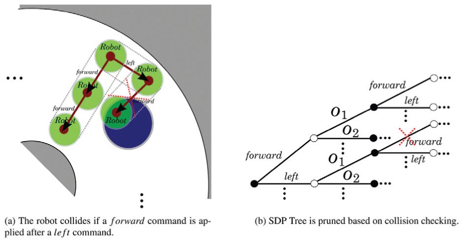
We use the range sensor to detect obstacles and measure their position relative to the robot. The position of the robot relative to C is still estimated probabilistically as before. When control commands are being planned, it is possible to predict if the robot will collide with obstacles (see Figure 16a), independently of its position relative to C. The branches of the search tree that cause collision are pruned (Figure 16b). Note that collision prediction can be done at the precision level provided by the range sensor, so that commands may allow the robot to traverse cells that are partially occupied by obstacles.
Integrating collision checking into the confirmation process.
A policy generated with Stochastic Dynamic Programming (SDP) with Imperfect State Information might be described as a tree that relates state beliefs, controls and observations. Our main idea to deal with motion constrains is to prune branches of this tree corresponding to controls yielding to a collision (see Figure 16b). In the planning and execution stages the robot just takes into account collision-free controls, and therefore this allows us to still use the transition model that we have been using so far without the necessity to recompute it integrating the obstacles; indeed, the location of the obstacles in the cellular decomposition with respect to the target, in both the planning and execution stages, is unknown.
During the execution of a sequence of commands we can predict if obstacles occlude C by combining the knowledge of the position of the robot relative to the obstacles with the estimated direction of C. In the absence of obstacles, our method uses a Bayes filter to update the probabilistic model of the position of the robot, integrating controls in a prediction step and observations in an update step. Now, if C is occluded by obstacles, only the prediction step is used to compute the probabilistic model. If the robot reaches a position where C is occluded, a new plan is generated from the probabilistic model computed with the prediction step only, temporarily ignoring the observations when updating the position distribution, and just applying the transition model until C is no longer occluded. It is important that the planner may send the robot to positions where the target is not visible. Otherwise, the range of valid paths could decrease too much, even to the point where the workspace is disconnected (see Figure 17).
If we do not allow the robot to reach regions
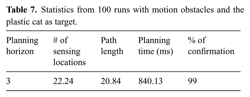
In a first set of runs, we tested our method with obstacles that only produce motion constraints, pruning branches of the search tree yielding to collision. The target is the plastic cat of Experiment #1, with three obstacles placed around it as shown in Figure 18. Table 7 gives the average measurements over 100 runs with planning horizon
Motion obstacles around the target (plastic cat) in the virtual environment.
Statistics from 100 runs with motion obstacles and the plastic cat as target.
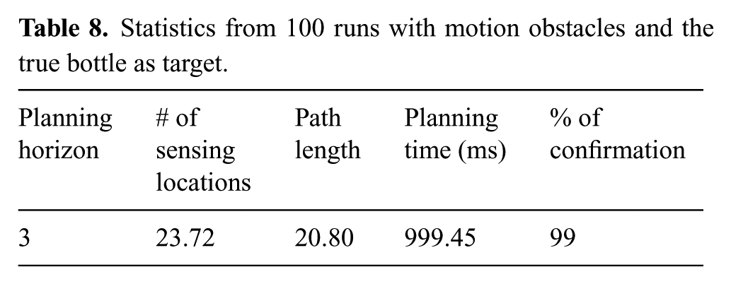
In our second set of runs, the robot is given the task of confirming the presence of the true bottle of Experiment #2. In that experiment (without obstacles) the robot had a tendency to move around the bottle in a clockwise direction, as shown in Figure 10c. Now three obstacles (shown in pink) that produce motion obstructions are included with one of them blocking the clockwise path of the robot. A sample path followed by the robot in the presence of these three obstacles is shown in Figure 19a (the yellow disc is the final position of the robot). Figure 19b shows another path, where the robot starts moving to the right, next it moves forward (into a cell that is partially occupied by an obstacle), but it then moves backwards in order to avoid collision and keeps moving around the bottle until detection is achieved. Table 8 gives average measurements over 100 runs. Again, as expected, there is a neat increase in the number of sensing locations, path length, and planning time, relative to the results shown in Table 4 of Experiment #3. However, the confirmation rate is still very good.
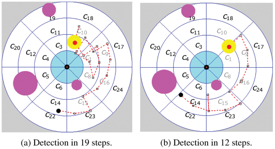
Sample paths for the true bottle while avoiding motion obstacles.
Statistics from 100 runs with motion obstacles and the true bottle as target.
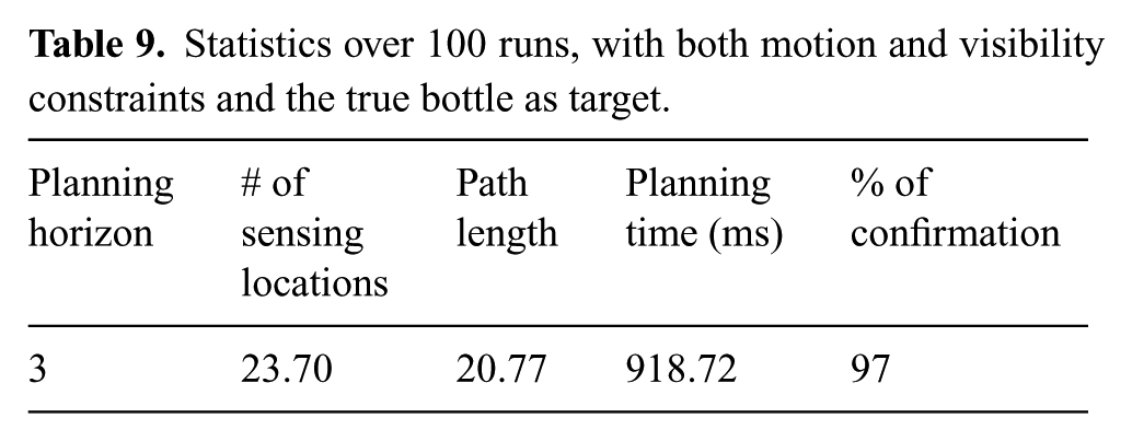
In our third set of runs we repeated the bottle set experiment, but now one of the three obstacles (the one in the inner ring of the cell decomposition) also produces visibility constraints (see Figure 20a and Figure 20b). In this case, whenever it is detected that C is occluded, only the prediction step is used to update the probabilistic model of the robot position relative to C. A sample path is shown in Figure 21, with robot positions where occlusion occurs marked by black “x”. The size of the occluding obstacle relative to the length of a motion step allows the robot to escape from the zone where occlusion takes place in two steps. Table 9 shows statistics over 100 trials. The results are quite similar to those obtained when only motion obstacles were present. However, the confirmation rate is marginally smaller.
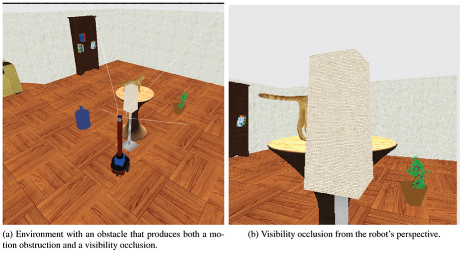
Experiment with both motion obstructions and visibility occlusions.
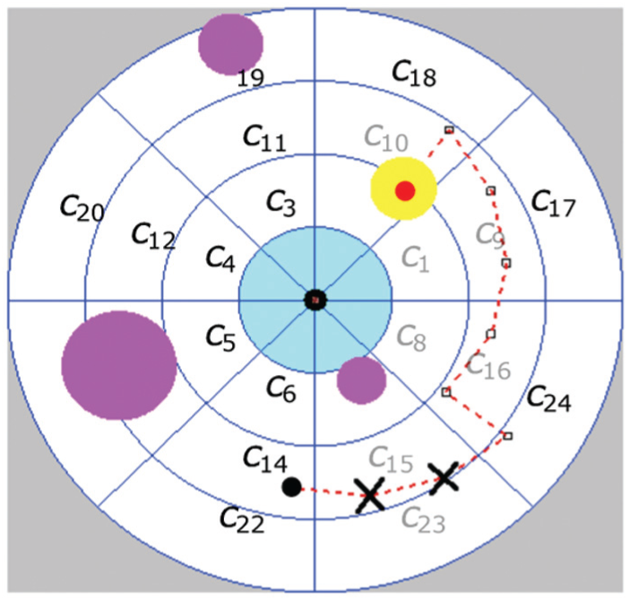
Sample path in the presence of an obstacle creating occlusion constraints.
Statistics over 100 runs, with both motion and visibility constraints and the true bottle as target.
8. Experiments with a real robot
8.1. General setting
In this section we present five experiments carried out with a real robot. The goal of these experiments is to further assess our approach. All our experiments took place in the Robotics Laboratory at CIMAT, shown in Figure 22.
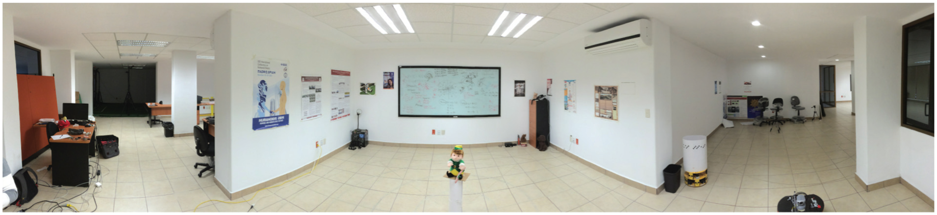
Laboratory environment for Experiments #5 through #9.
Our robot is a Pioneer P3-DX (a differential-drive robot) equipped with a USB camera as our visual sensor and a Sick-LMS200 range sensor. The robotic system and its software architecture are presented in more detail in Appendix C. The object to be identified is placed at the center of a rectangular support table (see center of Figure 22). The camera is used to take images that are fed into the target detector. The range sensor is used to keep the robot at an adequate distance from the support table to avoid collision with it and to maintain the candidate object within the field of view of the camera. The range sensor is also used to estimate the direction of the object C.
In the presented experiments we will vary two sets of parameters. Parameters in one set are related to the planner: planning horizon N and number of cells in the decomposition. Parameters in the other set are related to the environment and/or the target detector: illumination, scene background, textures, sizes, and colors of the targets, size of the sets of images used to train the detector and generate the observation models, and number of cells used to train the detector.
In Experiments #5, #6 and #7, the planner uses the 24-cell decomposition shown in Figure 1. In Experiments #8 and #9 it uses a reduced version of this decomposition with only 16 cells, obtained by removing the outer ring of cells. For each target T, the detector
In all experiments, the estimated direction of the center of the candidate object C is computed as follows. The laser scan of the range sensor intercepts the support of C. The two depth discontinuities corresponding to the two sides of this support are detected and the middle direction between them is the estimated direction.
As with the experiments in simulation, in all the statistics tables shown below, the average numbers of sensing locations, path lengths and planning times are computed only over the runs that achieve confirmation.
8.2. Experiment #5: A dark dog plush
The main purpose of this experiment is to test the ability of our system to confirm the presence of a target in a real-world scene. The target is the dog plush shown in Figure 23a. It has uniform texture and dark color. Only 40 images were used to train
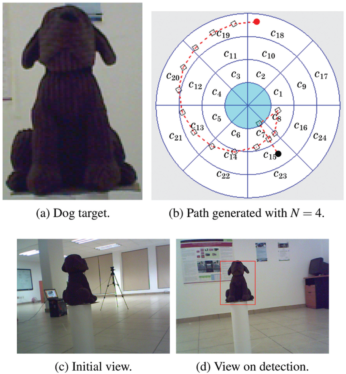
Illustrations for Experiment #5.
We experimented with planning horizons
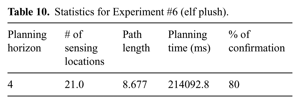
Statistics for Experiment #6 (elf plush).
The imperfect results obtained in this experiment led us to perform experiments with larger training sets of images under diverse illumination conditions, as reported below.
8.3. Experiment #6: A multicolor elf plush
This two main purposes of this experiment are to better analyze the impacts both of the choice of the planning horizon N and of the number of images used to train
The target T is the multicolor elf plush shown in Figure 24a. Initially the detector was trained (as in Experiment #5) on 40 images taken from within cell
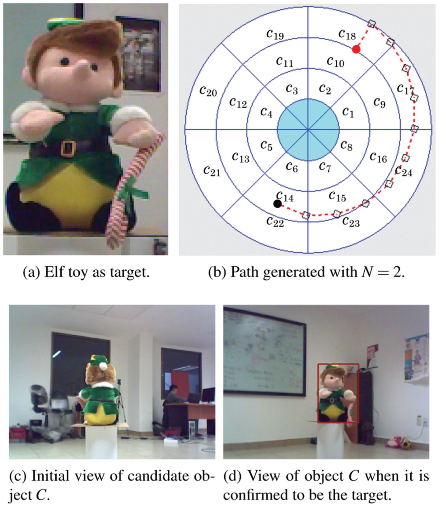
Illustrations for Experiment #6.
Figure 24b plots the path followed by the robot in a run with
Table 11 shows statistics collected for each value of N. Each line of the table was obtained over 10 runs with different initial positions of the robot within cell
Statistics for Experiment #6 (elf plush).

To test this hypothesis, we re-trained the detector
Statistics for Experiment #6 (elf plush) with enhanced training of the detector.
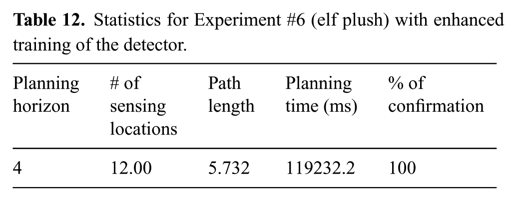
The number of steps before confirmation is roughly the same as those reported above for Experiments #1, #2, and #4 and observed for other experiments. In Experiment #5 a slightly larger number of steps was needed to confirm the target, despite the combination of lack of distinctive features of the dog plush, poor illumination of the scene, and small size of the training set of images. This suggests that the resolution of the cell decomposition and the step size, which has been the same for these experiments, is a key determinant of the number of steps. Hence, it may be possible to set a much smaller limit on the total number of steps, before the planner decides that a candidate object C is not the target. This would avoid wasting too much time when the candidate object C is not the target, without impacting the reliability of the confirmation process.
8.4. Experiment #7: Changes in illumination
This experiment has been directly inspired by Experiment #5, which was carried out with reduced illumination. Its purpose is to analyze the impact of variations in illumination conditions between the training and the execution phases.
The target is again the elf plush used in Experiment #6 and shown in Figure 24a. We used the same trained detector and observation model as in Experiment #6. They were both obtained with the illumination conditions of Figure 25a (1650 lux) 2 . Here, we perform two sets of additional runs with the reduced illumination conditions shown in Figure 25b (495 lux) and Figure 25c (16 lux).
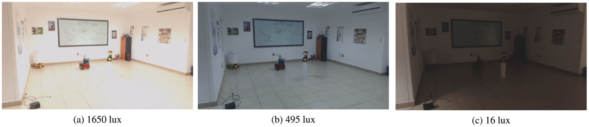
The same scene and target (elf plush) with three different illuminations (Experiment #7).
Table 13 shows the obtained statistics collected for each illumination over 10 runs, with random initial positions of the robot in cell
Statistics for Experiment #7 (variations in illumination).
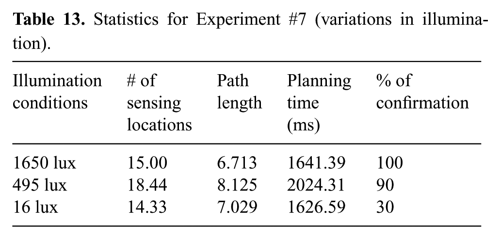
It is interesting to note that when confirmation is achieved with 16-lux illumination, the average number of sensing locations and the path length are similar in magnitude to those obtained in the 1650-lux and 495-lux scenarios. This suggests that with 16-lux illumination, the subset of
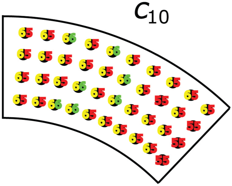
At each position the left number is the score
Detection methods may exist that are more robust to variations in illumination conditions than the deformable part model algorithm used in our detector, or better suited in poorly illuminated scenes. If it is known in advance that the illumination conditions during execution runs are likely to be poor or can differ widely from those during training, such a method should then be used in our system.
8.5. Experiment #8: Woodcraft of a jaguar head
The main goal of this experiment is to test the performance of the system with fewer cells in the decomposition X, when the target is smaller in size.
The target is the colorful woodcraft of a jaguar head shown in Figure 27a. It is smaller in overall size than the dog and elf used in previous experiments. For this reason we reduced the number of cells in the decomposition to 16 by removing the outer ring (8 cells) from the 24-cell decomposition shown in Figure 1.
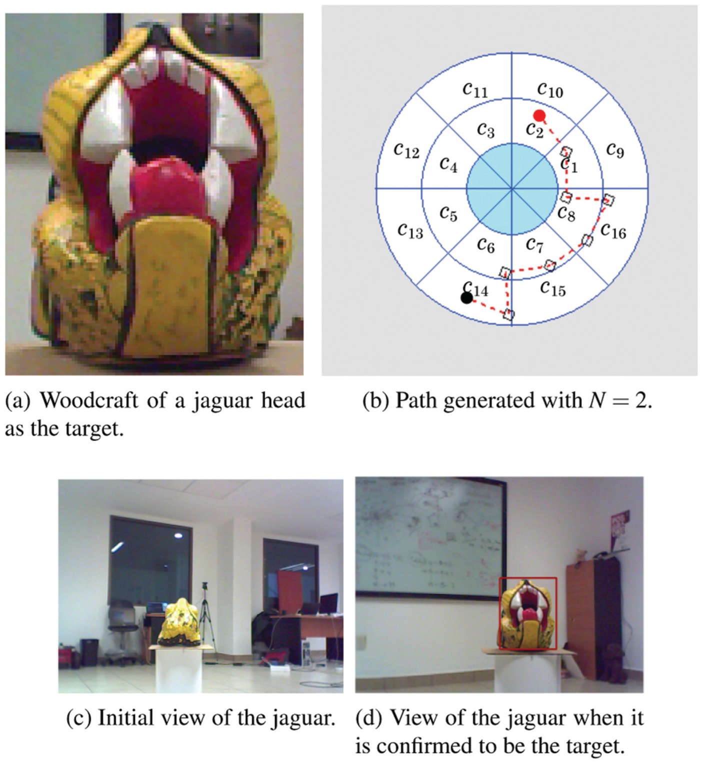
Illustrations for Experiment #8.
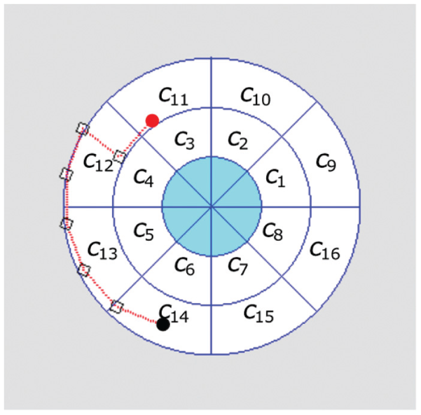
Path generated with
The detector was trained on 40 sample images using
Observation model
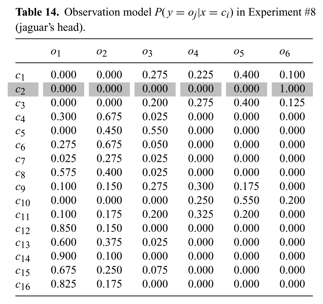
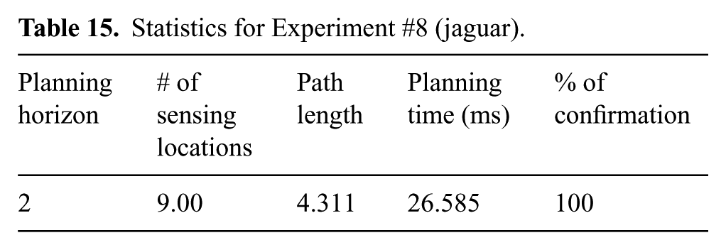
The smaller number of cells allows for a smaller planning horizon N, which we set to 2. Table 15 presents statistics collected over 10 runs with different initial positions of the robot within cell
Statistics for Experiment #8 (jaguar).
This result led us to perform the same experiment with the larger elf plush used in Experiment #6, i.e. with the same 16-cell decomposition as above and
Statistics for Experiment #8 (elf plush with 2-ring 16-cell decomposition).
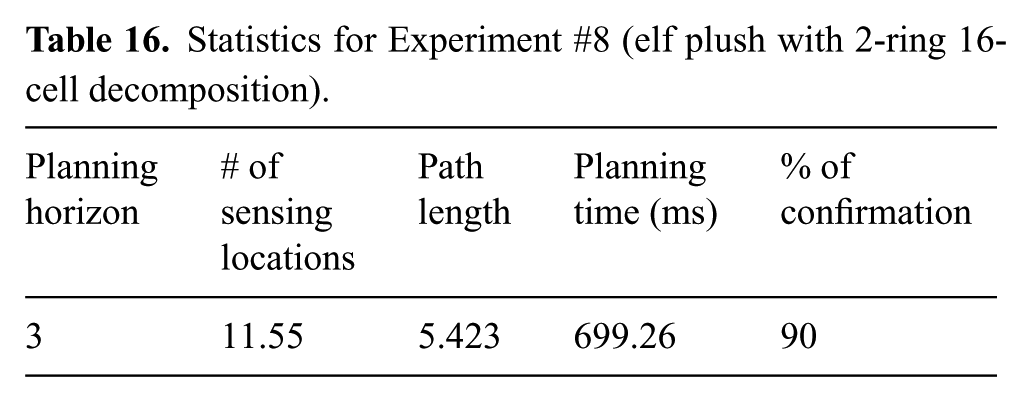
This comparison indicates that the size of the decomposition should be adapted to the size of the target. With targets larger than those used our experiments, one might have to use decompositions with 2 or 3 rings with larger inner and outer circles. In some cases (e.g. large elongated objects) non-circular decompositions may be more suitable. Extension 2 shows a run of this experiment at 1x speed.
8.6. Experiment #9: Detector trained over two adjacent cells
The purpose of this experiment is to test our system when the detector
The target is again the jaguar’s head shown in Figure 27a, with the same 16-cell decomposition as in Experiment #8. The detector
Observation model
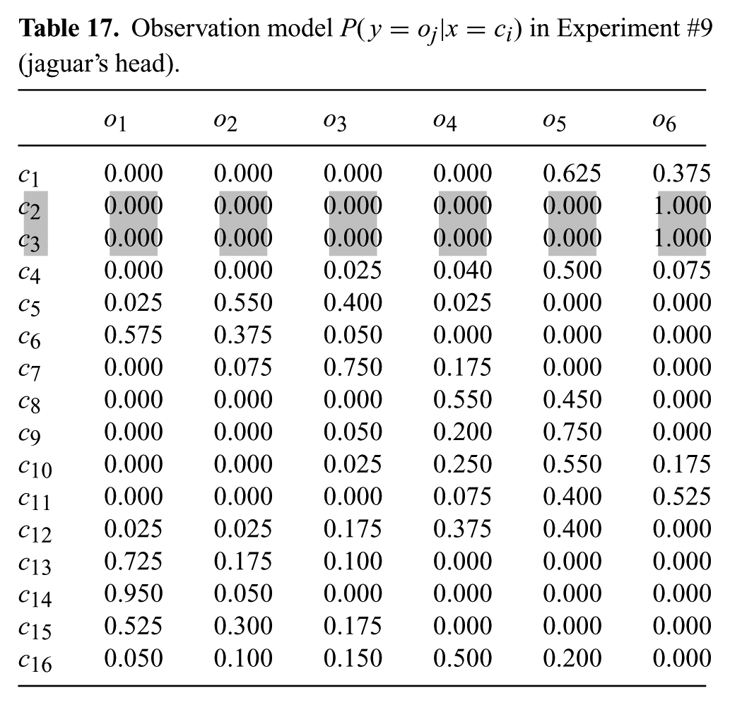
Table 18 shows statistics collected over 10 runs, with different initial positions of the robot within cell
Statistics for Experiment
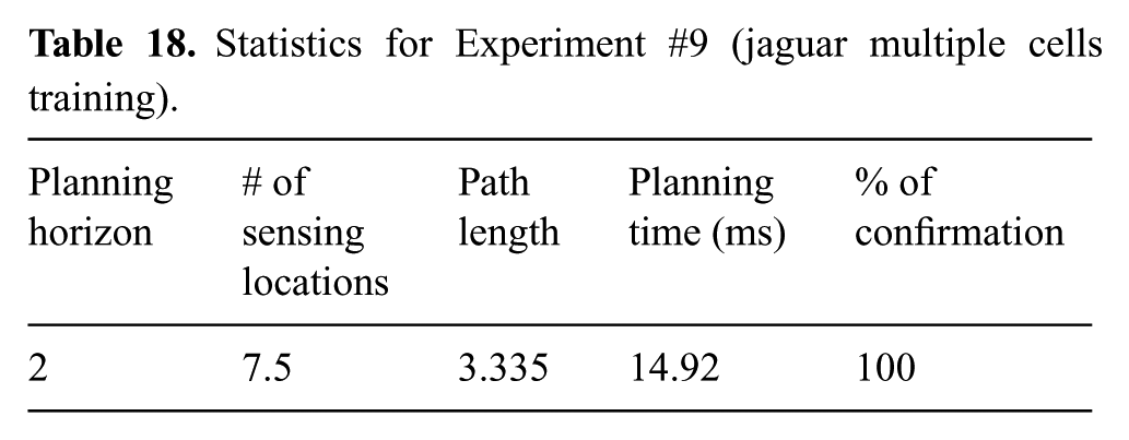
Training the detector over a larger number of cells may speed up confirmation in some cases, but may not always be suitable. If the diversity of viewpoints increases, the detector may require more images from each cell to be able to return high scores from each one. Moreover, if several objects have the same appearance from some viewpoints (as in Experiment #2 with two similar bottles), then incorrect confirmation of the target’s presence will become more likely. Our ability to train the detector in cells where distinctive features of the target are visible would be reduced or even lost.
The pertinence of using a static detector trained from multiple viewpoints, or a mobile robot using multiple detectors, or a mobile robot using a single detector, depends on the appearance of the target. If the target has only one small feature that differentiates it from similar objects, then both having a single detector which works well and having a sensor with high mobility is essential. If the target has several distinctive features visible from across several viewpoints, then multiple detectors may be preferable. In addition, if at least one distinctive feature is visible from any viewpoint (a rare case in practice), then a static detector would work. In general, the mobility of the sensor makes it possible to reduce the number of viewpoints needed to train the detector.
Remark: As a final note regarding all the experiments, selecting the ideal value of the threshold
9. Conclusions and further work
We have presented and tested a new approach allowing a mobile robot equipped with visual sensors to confirm that a candidate object C is a given target T using an imperfect target detector. Our main contribution is a POMDP formulation of the problem, which mixes localization of the robot relative to C and confirmation that C is the target T. To confirm the target’s presence while avoiding false positives, the robot must achieve a twofold condition: (1) it must reach a position where the target detector has high probability to return a high confidence score, and (2) the detector must actually return a high confidence score on the image taken at this position.
Motion strategies are computed as policies with given horizons using Stochastic Dynamic Programming (SDP) with Imperfect State Information. Computing exact solutions in SDP with Imperfect State Information does not scale well with the planning horizon, but our experiments show that space decompositions with relatively few cells suffice. Such decompositions do not require very long horizons. Moreover, we have introduced a gain function
We have implemented our method and tested it both in simulation and with a real robot. In this paper, we have presented results obtained in nine different experiments (four in simulation and five with a real robot). Some of these experiments include several significant variants aimed at further understanding some results or validating certain hypotheses. Overall, these experiments demonstrate that our system is efficient and reliable under a broad range of situations. In particular, they show that it tolerates similar-looking targets and candidate objects, variations in scene illumination, non-uniform scene backgrounds, targets with various colors, shapes, and textures, relatively small training sets of images, and large errors in the estimated direction of the candidate object’s center. They also indicate that the sizes (24 and 16 cells) of our cell decompositions are appropriate for the small targets we have considered, that planning horizons 2 and 3 work well with these decompositions and the additional gain function
Our goals for future research include the following;
In addition to these research goals, we are also interested in a more practical goal: building a robot that can routinely search for user-specified targets in an indoor environment.
Footnotes
Appendices
Funding
The author(s) disclosed receipt of the following financial support for the research, authorship, and/or publication of this article: Rafael Murrieta-Cid was supported in part by Conacyt grant No. 220796.
Notes
References
Supplementary Material
Please find the following supplemental material available below.
For Open Access articles published under a Creative Commons License, all supplemental material carries the same license as the article it is associated with.
For non-Open Access articles published, all supplemental material carries a non-exclusive license, and permission requests for re-use of supplemental material or any part of supplemental material shall be sent directly to the copyright owner as specified in the copyright notice associated with the article.