Swarm assignment and trajectory optimization using variable-swarm,distributed auction assignment and sequential convex programming

Abstract

This paper presents a distributed, guidance and control algorithm for reconfiguring swarms composed of hundreds to thousands of agents with limited communication and computation capabilities. This algorithm solves both the optimal assignment and collision-free trajectory generation for robotic swarms, in an integrated manner, when given the desired shape of the swarm (without pre-assigned terminal positions). The optimal assignment problem is solved using a distributed auction assignment that can vary the number of target positions in the assignment, and the collision-free trajectories are generated using sequential convex programming. Finally, model predictive control is used to solve the assignment and trajectory generation in real time using a receding horizon. The model predictive control formulation uses current state measurements to resolve for the optimal assignment and trajectory. The implementation of the distributed auction algorithm and sequential convex programming using model predictive control produces the swarm assignment and trajectory optimization (SATO) algorithm that transfers a swarm of robots or vehicles to a desired shape in a distributed fashion. Once the desired shape is uploaded to the swarm, the algorithm determines where each robot goes and how it should get there in a fuel-efficient, collision-free manner. Results of flight experiments using multiple quadcopters show the effectiveness of the proposed SATO algorithm.

1. Introduction

Motion planning (often called guidance in the aerospace community) and feedback control of multi-agent systems have been major areas of research over the past decades. The majority of this work focused on swarm robotics (Alonso-Mora et al., 2012; Cheah et al., 2009; Earl and D’Andrea, 2005; Hsieh et al., 2008; Jadbabaie et al., 2003; Kingston and Egerstedt, 2010; Milutinović and Lima, 2006; Yu et al., 2015; Zhao et al., 2011). However, in recent years the idea of multi-agent systems has been extended to spacecraft (Alfriend et al., 2009; Breger and How, 2007; Campbell, 2003, 2005; Hadaegh et al., 2014; Scharf et al., 2003, 2004; Vaddi et al., 2005; Zanon and Campbell, 2006). The most recent idea is to fly a swarm containing a large number (hundreds to thousands) of femtosatellites (100-gram-class spacecraft) (Hadaegh et al., 2014).

For a swarm to have a cost benefit compared to a monolithic agent or a smaller formation, the individual agents need to be smaller and cheaper. Due to their small size and low cost, the agents in a swarm have limited actuation, communication, and computation capabilities, which require the guidance and control algorithms of the swarm to be both fuel and computationally efficient. Swarms of agents create interesting challenges in guidance and control due to the large number of agents, the small size of each individual agent, and the complicated dynamics. Specifically, the large number of vehicles moving in three dimensions makes collision avoidance a major challenge (Morgan et al., 2012, 2014). Also, the limited computation and communication capabilities of each agent require the swarm reconfiguration algorithm to be very simple so that it can be run on board each small robot or vehicle in real time.

The swarm reconfiguration problem consists of two parts: assignment and trajectory generation. The assignment problem consists of finding the optimal mapping from a set of agents to a set of targets or tasks in order to minimize the total cost of interest. This problem has been well researched and many methods exist for finding the optimal assignment, including the Hungarian algorithm (Kuhn, 1955) and iterative methods (Bertsekas, 1981; Hung, 1983). The drawback to many of these algorithms is that they are centralized with respect to communication and computation. On the other hand, the auction algorithm (Bertsekas and Castanon, 1991; Bertsekas, 1992) possesses a distributed nature suitable for distributed systems. More recent research on the auction algorithm (Choi et al., 2009; Zavlanos et al., 2008) has shown that it can be implemented in a distributed manner. In contrast with the prior work, one important aspect of the assignment algorithm in this paper is its versatility to adapt to information, specifically collision avoidance and disconnected communication networks.

The second part of the swarm reconfiguration is optimal trajectory generation and collision avoidance. This part requires an algorithm that can solve the nonlinear optimization that minimizes the cost of the trajectory while satisfying collision avoidance and dynamic constraints. The trajectory optimization has been solved using a variety of methods, including mixed integer linear programming (Richards et al., 2003), pseudospectral methods (Ross and Fahroo, 2003), convex programming (Schulman et al., 2013), and sequential convex programming (SCP) (Morgan et al., 2014).

In this paper, we simultaneously solve both the target assignment and trajectory optimization problems using: a variable-swarm, distributed auction assignment (VSDAA), which allows the swarm size to change over time, to solve the assignment problem; and our prior work on SCP (Morgan et al., 2014) to solve the trajectory optimization. Additionally, we integrate these algorithms using model predictive control (MPC) (Bemporad and Morari, 1999; Mayne et al., 2000) in order to run the algorithms in real time and on swarms with distributed communication networks. The integration with the trajectory optimizer is what allows the auction algorithm the ability to adjust its assignment based on collisions that were previously undetected.

The contributions of this paper, compared with the existing literature including our own work (Morgan et al., 2014), are in the development of VSDAA, its integration with trajectory optimization in the MPC-SCP formulation, and the convergence proof for SCP as well as in the experimental validation using multiple quadrotors. The variable-swarm characteristic means that VSDAA can adapt the number of targets in the assignment to match the number of agents. This is incredibly useful when the number of agents in the swarm changes. In the case of a significant loss of agents due to an external object or fuel/battery depletion, VSDAA would adjust the number of targets to match the number of remaining agents and the agents would fill in the gap left by the external object. This allows the swarm to handle the loss of a significant number of agents and still maintain the desired shape. On the other hand, VSDAA will also increase the number of targets if there are more agents than targets. This is a situation that will break a typical auction algorithm (Bertsekas and Castanon, 1991; Bertsekas, 1992; Choi et al., 2009; Zavlanos et al., 2008) since the agents cannot all be assigned to a target so they bid indefinitely. Also, it should be noted that VSDAA can handle an arbitrary distribution shape of targets, as opposed to the use of uniform target distributions (Yu et al., 2015).

Another contribution is that the SCP method is shown to converge to a Karush–Kuhn–Tucker (KKT) point (Boyd and Vandenberghe, 2004; Ruszczynski, 2006) of the nonconvex program. This proof shows that once a feasible solution is found, the sequence of optimal solutions resulting from the convex programs will converge. Additionally, the trajectory to which they converge satisfies the KKT conditions, which are necessary conditions for an optimal trajectory.

Additionally, the implementation of VSDAA with SCP using MPC allows an assignment to be achieved even in a disconnected communication network. Since the assignment is updated throughout the reconfiguration, the distance-based swarm communication network will be different every time an assignment is computed. Therefore, the agents do not need to be fully connected to every other agent at all times. In fact, if two agents from separate, disconnected networks are assigned to the same target, they will eventually move close enough to become connected and will be assigned to different targets.

The result of the MPC implementation of VSDAA and SCP is the swarm assignment and trajectory optimization (SATO) algorithm. SATO, the main algorithm of this paper, is distributed in both communication and computation, and provides near-optimal, collision-free trajectories for swarm reconfiguration. In contrast to other methods that simultaneously solve the assignment and trajectory optimization (Turpin et al., 2014), SATO uses SCP as underlying trajectory optimization, which allows it to handle complex dynamic environments. Additionally, this algorithm works with disconnected communication networks and is robust to the loss or gain of a significant number of agents. Finally, the model predictive control formulation allows SATO to run on board each agent and provides robustness to unmodeled disturbances. A preliminary version of this paper was previously presented at a conference (Morgan et al., 2015), but this paper adds significant results of experimental validation along with detailed description of dynamic modeling and nonlinear control design.

The paper is organized as follows. In Section 2, the swarm reconfiguration problem is formulated as a constrained, nonlinear optimal control problem and converted to a nonlinear optimization. In Section 3, the swarm reconfiguration problem is broken into an assignment problem and a trajectory optimization problem. Then, the assignment is solved using VSDAA. In Section 4, the trajectory optimization problem is converted to a convex optimization and the SCP algorithm is described. Additionally, the SCP algorithm is shown to converge to a trajectory that satisfies the KKT conditions of the nonconvex problem. In Section 5, MPC is used to integrate VSDAA and SCP, and to implement a finite horizon so that the resulting algorithm, SATO, can be run on board each agent in real time with a disconnected communication network. In Section 6, SATO is run for both a two-dimensional (2-D) double integrator dynamics scenario and a three-dimensional (3-D) relative orbit dynamics scenario. The results of the two scenarios are analyzed and discussed. In Section 7, we elaborate on our experimental setup, the feedback control law design to track the desired trajectories obtained by SATO, and the experimental results.

2. Problem statement

In this section, the optimal swarm reconfiguration is presented as a continuous, finite horizon optimal control problem. The swarm reconfiguration involves the transfer of hundreds to thousands of agents from their current shape to a desired shape while satisfying various constraints, such as collision avoidance, and minimizing the total fuel used during the transfer. A visualization of a swarm reconfiguration and communication networks is shown in Figure 2.

Figure 1(a) shows a visualization of the swarm reconfiguration problem. The agents begin at their current positions (green) and move towards the desired formation (red). The agents are interchangeable so any agent can go to any target. In Figure 1(b), the connectedness of various agents is shown. The dashed arrows represent communication links between the agents and the different colors represent different communication networks. In other words, the blue agents are connected to the other blue agents (agents 1 and 4) but not to the red agents (agents 2 and 5). Two agents that have a communication link between them are called neighboring agents (agents 7 and 8).

Fig. 1.

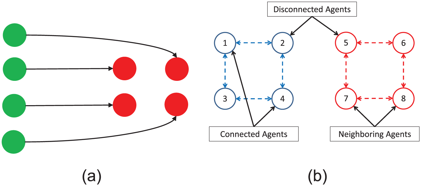
Visualization of problem statement and communication networks. (a) Visualization of a swarm reconfiguration. (b) Visualization of connected and disconnected networks. Dashed lines represent communication links.

2.1 Nonlinear optimal control problem

The objective of the optimal swarm reconfiguration is to minimize the $L_{1}$ -norm of the control input. Therefore, we can define the swarm reconfiguration as follows.

Problem 1 (Constrained, nonlinear optimal control).

\begin{matrix} min_{u_{j} (t), j = 1, \dots, N} \sum_{j = 1}^{N} \int_{0}^{t_{f}} ∥ u_{j} (t) ∥_{q} dt subject to \end{matrix}

(1)

\begin{matrix} {\overset{\cdot}{x}}_{j} (t) = f (x_{j} (t)) + B u_{j} (t)) \forall t \in [0, t_{f}], \\ j = 1, \dots, N \end{matrix}

(2)

∥ u_{j} (t) ∥_{r} \leq U_{\max} \forall t \in [0, t_{f}], j = 1, \dots, N

(3)

\begin{matrix} ∥ G [x_{j} (t) - x_{i} (t)] ∥_{2} \geq R_{col} \forall t \in [0, t_{f}], i < j, \\ j = 1, \dots, N - 1 \end{matrix}

(4)

x_{j} (0) = x_{j, 0}, j = 1, \dots, N

(5)

x_{j} (t_{f}) \in X_{f}, j = 1, \dots, N

(6)

where $B = [0_{3 \times 3} I_{3 \times 3}]^{T}$ , $G = [I_{3 \times 3} 0_{3 \times 3}]$ , $x_{j} = (ℓ_{j}^{T}, {\overset{\cdot}{ℓ}}_{j}^{T})^{T}$ , $ℓ_{j} \in ℝ^{n}$ is the position vector of agent $j$ , $x_{j, 0}$ is the initial state of agent $j$ , $u_{j}$ is the control vector of agent $j$ , and $N$ is the number of agents in the swarm. Equations (2)–(5) represent the dynamics constraint, maximum control constraint, collision avoidance constraint, and initial state constraint, respectively, with $U_{\max}$ being the maximum control magnitude and $R_{col}$ being the minimum allowable distance between two agents. Equation (6) represents the terminal state constraint with $X_{f}$ being a set of $M$ discrete points in $ℝ^{n}$ . This constraint is what introduces the need for solving for the optimal assignment and differentiates this paper from our prior work (Morgan et al., 2014), where individual terminal state assignments were given.

Remark 1 (Norms) The norms used in equations (1) and (3), $∥ \cdot ∥_{q}$ and $∥ \cdot ∥_{r}$ , respectively, are dependent on the hardware used on board the agents. In this paper, we use $q = 1$ and $r = \infty$ . However, the convex optimizations are valid for $q, r \in {1, 2, \infty}$ .

Remark 2 (Fixed terminal time) The optimizations used in this paper all have a fixed terminal time. This is due to the fact that the swarm is trying to reconfigure to a specific shape so the agents need to arrive at their terminal positions at the same time. If some agents arrive earlier than others, they will either drift off of their target position or require extra cost to maintain their position in the presence of dynamics. Additionally, the trajectories are generally cheaper for longer reconfiguration times so having some agents arrive earlier than others usually increases the cost for those agents arriving early.

2.2. Convexification of differential equations

In this section, the dynamics constraints in equation (2) are converted to affine equality constraints. This is done by linearizing equation (2) and discretizing Problem 1. This results in a finite number of linear equality constraints, which are acceptable in a convex programming problem.

In order to rewrite the dynamics in equation (2) as a constraint that can be used in a convex programming problem, these equations must first be linearized about the nominal trajectory $x_{j}^{0}$ . Linearizing equation (2) yields

{\overset{\cdot}{x}}_{j} = A (x_{j}^{0}) x_{j} + B u_{j} + z (x_{j}^{0})

(7)

where $A (x_{j}^{0}) = {\frac{\partial f}{\partial x_{j}} |}_{x_{j}^{0}}$ and $z (x_{j}^{0}) = f (x_{j}^{0}) - {\frac{\partial f}{\partial x_{j}} |}_{x_{j}^{0}} x_{j}^{0}$

The next step in the process of converting equation (2) into a constraint that can be used in convex programming is to convert the ordinary differential equation in equation (7) to a finite number of algebraic constraints. In order to do this, the problem is discretized using a zero-order-hold approach such that

u_{j} (t) = u_{j} [k], t \in [t_{k}, t_{k + 1}), k = k_{0}, \dots, T - 1

(8)

where $t_{f} = T Δ t$ , $T$ is the number of discrete time steps, $t_{0} = 0$ , $t_{T} = t_{f}$ , and $Δ t = t_{k + 1} - t_{k}$ for $k = k_{0}, \dots, T - 1$ . This method of discretization reduces equation (7) to

\begin{matrix} x_{j} [k + 1] = A_{j} [k] x_{j} [k] + B_{j} [k] u_{j} [k] + z_{j} [k], \\ k = k_{0}, \dots, T - 1, j = 1, \dots, N \end{matrix}

(9)

where $x_{j} [k] = x_{j} (t_{k})$ , $u_{j} [k] = u_{j} (t_{k})$ , and

\begin{matrix} A_{j} [k] = e^{A (x_{j}^{0} (t_{k})) Δ t}, B_{j} [k] = \int_{0}^{Δ t} e^{A (x_{j}^{0} (t_{k})) τ} B d τ, \\ z_{j} [k] = \int_{0}^{Δ t} e^{A (x_{j}^{0} (t_{k})) τ} z (x_{j}^{0} (t_{k})) d τ \end{matrix}

(10)

Now that the nonlinear, continuous-time equations of motion from (2) have been rewritten as linear, finite dimensional constraints in (9), they can be used in a convex programming problem. The constraints from equations (3)–(6) can be written in discretized form as

\begin{matrix} ∥ u_{j} [k] ∥_{\infty} \leq U_{\max} k = k_{0}, \dots, T - 1, \\ j = 1, \dots, N \end{matrix}

(11)

\begin{matrix} ∥ G (x_{j} [k] - x_{i} [k]) ∥_{2} \geq R_{col} k = k_{0}, \dots, T, i < j, \\ j = 1, \dots, N - 1 \end{matrix}

(12)

x_{j} [0] = x_{j, 0}, j = 1, \dots, N

(13)

x_{j} [T] \in X_{f}, j = 1, \dots, N

(14)

Note that the only constraints that do not satisfy the requirements of convex programming are equations (12) and (14). These constraints will be modified in the following sections so that the problem can be efficiently solved using convex programming.

3. Distributed optimal target assignment

In this section, the nonlinear optimal control problem (Problem 1) is broken into two parts: an optimal assignment problem and an optimal trajectory-planning problem. This separation allows us to rewrite the terminal constraints in equation (14), which are nonconvex and require the problem to include integer variables. By solving an assignment problem to determine the terminal states of each agent, the remaining trajectory-planning problem can be approximated by a convex program and efficiently solved.

Claim 1 (Assignment) If the terminal set ( $X_{f}$ ) is a set of points with every pair of points separated by a safe distance ( $R_{col}$ ), then the constraints $x_{j} [T] \in X_{f}$ (14) and $∥ G (x_{j} [T] - x_{i} [T]) ∥_{2} \geq R_{col}$ ((12) at $k = T$ ) can be equivalently written as

x_{j} [T] \in X_{f}, x_{j} [T] \neq x_{i} [T], \forall j \neq i

(15)

Now, the assignment problem can be written as shown below.

Problem 2 (Assignment problem)

min_{x_{j, f}, j = 1 \dots N} \sum_{j = 1}^{N} C (x_{j, 0}, x_{j, f}) subject to

(16)

x_{j, f} \in X_{f}, x_{j, f} \neq x_{i, f}, \forall j = 1 \dots N, \forall i \neq j

where $C (x_{0}, x_{f})$ is the cost required for an agent to go from $x_{0}$ to $x_{f}$ .

The solution to the assignment problem (Problem 2) will yield the desired terminal points for each agent ( $x_{j, f}$ ), which are then used to formulate the following terminal constraint for the trajectory optimization problem

x_{j} [T] = x_{j, f}, j = 1, \dots, N

(17)

The resulting trajectory optimization can be written as follows.

Problem 3 (Trajectory optimization)

\begin{matrix} min_{u_{j}, j = 1, \dots, N} \sum_{j = 1}^{N} \sum_{k = k_{0}}^{T - 1} ∥ u_{j} [k] ∥_{1} Δ t subject to \\ {(9), (11), (12), (13), (17)} \end{matrix}

(18)

Remark 3 (Assignment cost function) The assignment cost function ( $C_{auc} (x_{0}, x_{f})$ ) should approximate the optimal cost of solving Problem 5 so that the assignment and trajectory optimization are optimizing the same quantity. However, an exact solution to Problem 5 is difficult to obtain when calculating the optimal assignment due to the coupling between agents in the collision avoidance constraint. Therefore, the cost function used in Problem 2 should be the solution to Problem 5 without the collision avoidance constraint. The resulting problem is a decoupled convex program, which can be efficiently solved.

Remark 4 (Motion primitives and distance-based cost for assignment) In some cases, predetermined motion primitives (Paranjape et al., 2015) can be used as the cost function in Problem 2 to further simplify the calculations. These primitives allow the assignment cost to be calculated using simple algebraic functions, which greatly reduces the computation time when compared to solving an optimization for each robot-target pair. For example, when the dynamics are double integrator, a function of the distance between the initial and terminal points can be used as the assignment cost in equation (16) (e.g. $C (x_{j, 0}, x_{j, f}) \propto ∥ G (x_{j, 0} - x_{j, f}) ∥_{2}^{ν}$ ).

Remark 5 (Maximum fuel available) Since each vehicle (or robot) will have a limited amount of fuel (or energy), some targets might be unreachable. In order to ensure that a robot is not assigned to an unreachable target, every cost that exceeds the available fuel should be set to infinity or some sufficiently large number. This will ensure that every robot can reach its assigned target given its available fuel.

3.1. Distributed auction algorithm

To solve the assignment problem (Problem 2), an auction algorithm is used. This algorithm is typically used to solve a centralized assignment problem (Bertsekas, 1992; Bertsekas and Castanon, 1991), but its structure allows it to be implemented in a distributed manner (Zavlanos et al., 2008) even in some less desirable situations, including limited communication and changes in the number of agents.

In a typical auction algorithm, the computations can be centralized or decentralized, but the current bid prices, current highest bidders, and current bid for each agent must all be stored in shared memory that can be accessed by all of the agents. This requires all-to-all or all-to-one (star) communication, which is an impractical requirement of a large swarm. Additionally, the agents take turns bidding, which requires that each agent knows how many agents are in the swarm.

A distributed auction algorithm, VSDAA, is developed to solve the assignment problem for a swarm containing a varying number of agents that do not have all-to-all or all-to-one communication. VSDAA (Method 1) follows the same steps as a typical auction algorithm with a few exceptions. First, all of the computations are run in parallel and all of variables are stored locally (values for agent $i$ are denoted by superscript $i$ in Method 1). The bid prices of each agent ( $p^{i}$ ) are communicated to the neighboring agents and each agent stores the largest price received for each target (line 31). This introduces the possibility that agents are bidding based on outdated prices, but over time all of the agents that are connected on the communication graph will receive updated prices and bid appropriately. Finally, the number of target locations that agent $i$ is bidding on ( $m^{i}$ ) can be changed if the number of bids being received by agent $i$ is different than the number of target locations.

Method 1 Variable-swarm, distributed auction algorithm (VSDAA).
1: $X_{f} =$ terminal positions in desired shape
2: $c^{i} (s) =$ cost of agent $i$ choosing target $s$
3: $m^{i} =$ # of targets available for agent $i$ to bid on
4: $p^{i} = 0_{1 \times m^{i}}$
5: $p_{old}^{i} = - 1_{1 \times m^{i}}$
6: $j^{i} = 1$
7: $coun t^{i} = 0$ $i$
8:for all (run in parallel) do
9: while $coun t^{i} < 2 D_{net}$ do
10: if $\| p^{i} (j^{i}) \| > p_{old}^{i} (j^{i})$ ( $i$ is outbid) then
11: $m^{i} = max (m^{i}, \| {s \| p^{i} (s) \neq 0} \|)$
12: if $\| {s \| p^{i} (s) > 0} \| = m^{i}$ then
13: $m^{i} = \| {s \| p^{i} (s) > 0} \| + 1$
14: $p^{i} (1 : m^{i}) = - (\| p^{i} (1 : m^{i}) \| + ε)$
15: end if
16: $v^{i} = min_{s = 1 \dots m^{i}} (c^{i} (s) + \| p^{i} (s) \|)$
17: $j^{i} = \arg mi n_{s = 1 \dots m^{i}} (c^{i} (s) + \| p^{i} (s) \|)$
18: $w^{i} = min_{s = 1 \dots m^{i}, s \neq j^{i}} (c^{i} (s) + \| p^{i} (s) \|)$
19: $γ^{i} = w^{i} - v^{i} + ε$
20: $p^{i} (j^{i}) = \| p^{i} (j^{i}) \| + γ^{i}$
21: $coun t^{i} = 0$
22: else if $p^{i} \neq p_{old}^{i}$ (another agent is outbid) then
23: $m^{i} = max (m^{i}, \| {s \| p^{i} (s) \neq 0} \|)$
24: $coun t^{i} = 0$
25: else
26: $coun t^{i} = coun t^{i} + 1$
27: else if
28: $p_{old}^{i} = p^{i}$
29: Communicate $p^{i}$ to all agents in $N_{[i]}$
30: for $s = 1 \dots m^{i}$ do
31: $p^{i} (s) = min_{q \in \arg ma x_{q \in N_{[i]}} (\| p^{q} (s) \|)} (p^{q} (s))$
32: end for
33: end while
34: Optional: $m^{i} = \| {j \| p^{i} (j) \neq 0} \|$
35: Optional: Go back to line 4 and rerun with new $m^{i}$
36: $x_{i, f} = X_{f} (j^{i})$
37:end for

In VSDAA (Method 1), each agent runs the algorithm in parallel (line 8) and all computations are done locally. First, we assume that each agent knows the cost ( $c^{i} (j) = C (x_{i, 0}, X_{f} (j))$ ) of moving from its current location ( $x_{i, 0}$ ) to every target position ( $X_{f} (j)$ ). Then, the agents begin the bidding process. Each agent first checks to see if it has been outbid by another agent (line 10). If it has been outbid, it checks to see if the number of bids is equal to the number of targets ( $m^{i}$ ) in the assignment (line 12). If this is the case, the agent increases the number of targets used in the assignment by one (line 13) and increases the magnitude of the bid on each target (line 14) so that each agent has the opportunity to bid on the new target. Additionally, every bid is made negative so that every target becomes available. Then, the agent bids on one of the first $m^{i}$ target positions by choosing the target with the lowest total cost (line 16), which is composed of the fixed, predetermined cost ( $c^{i}$ ) and the variable, bidding cost ( $p^{i}$ ). Once the desired target ( $j^{i}$ ) for agent $i$ is chosen, the bid amount ( $γ^{i}$ ) is set as the difference between the cost of the two cheapest targets ( $v^{i}$ and $w^{i}$ ) with the addition of a small increment ( $ε$ ), which ensures that the bid price on any target is strictly increasing. Finally, the bid price of the chosen target is increased by the bid amount (line 20). The agent then resets its counter to zero. If the agent was not outbid, but some other bid has changed, the agent sets its counter to zero but does not go through the bidding calculations. If none of the bids have changed, the agent increases its counter by one (line 26). Finally, the agent stores its current bid estimates ( $p_{old}^{i}$ ), communicates its bid estimates to its neighbors, and updates its current bids based on the bids received from its neighbors. The neighboring agents of agent $i$ are defined by a distance-based communication network so the resulting neighborhood ( $N_{[i]}$ ) is closed ( $i \in N_{[i]}$ ) and the communication links are bidirectional ( $j \in N_{[i]}$ if and only if $i \in N_{[j]}$ ). The bidding process continues until the agent’s counter reaches twice the graph diameter (Harary, 1994) of the communication network ( $D_{net}$ ), which guarantees that no agents are bidding and an assignment has been achieved. In Method 1, |{·}| is used to denote the cardinality of a set.

3.2. Properties of variable-swarm, distributed auction assignment

In addition to distributing the computation and communication requirements of the auction algorithm, Method 1 also allows for the number of target locations to adjust based on the number of agents in the swarm. This is done by only using the bidding information so no additional consensus algorithm is needed to determine the number of agents. This is a very useful property when the number of agents in the swarm is large and the loss of some agents needs to be overcome to achieve the goal.

In Method 1, each agent keeps track of the number of targets it thinks the swarm needs ( $m^{i}$ ), which is the same as the number of agents it thinks are in the swarm. The number of targets can be increased during the algorithm (line 13) if an agent is about to place a bid and all of the $m^{i}$ targets already have been bid upon. Since an agent will only change its bid if it is outbid, every target that has been bid upon will have a bidder at all future times. Therefore, every target having a bid implies that there are $m^{i}$ agents in the swarm plus the agent that is bidding, and therefore is not assigned to a target. For this reason, $m^{i}$ is increased to allow enough targets for all of the agents. This can happen as many times as needed provided that $m^{i}$ does not exceed $M$ , which is the number of targets defined in $X_{f}$ .

In addition to increasing $m^{i}$ when there are more agents than expected, the algorithm will also adjust to having fewer agents than expected if it notices that some of the targets have not been bid upon. This case is more complicated because it may not be desirable in certain situations and cannot be detected until the bidding is finished. An assignment with more targets than agents can be solved by any auction algorithm, but in the case of swarm reconfiguration, it may not result in the desired shape if the number of agents is significantly less than the number of targets. Therefore, it may be desirable to either rerun the algorithm with the correct number of targets or update the number of targets needed for the next reconfiguration. This idea is shown in the optional step on line 34 where the agents adjust the number of targets in the assignment to be equal to the number of bids it received. This step is labeled optional because it might not be desirable to decrease the number of targets in certain situations: specifically, if the number of agents is not expected to change and the communication network may become disconnected. In this case, the algorithm will only see the bids of the agents that it is connected to and it will decrease the number of desired targets accordingly. In other words, the algorithm cannot distinguish between agents it cannot communicate with because they are disconnected and agents that have been lost.

Remark 6 (Desired targets ( $X_{f}$ )) VSDAA (Method 1) will access the first $m^{i}$ targets in $X_{f}$ based on how many agents it thinks are in the swarm. To achieve a desirable shape, $X_{f}$ should have two characteristics. First, the number of targets ( $M$ ) defined in $X_{f}$ should be large enough that $m^{i}$ never exceeds the number of targets defined. Second, Method 1 will access the first $m^{i}$ targets of $X_{f}$ . Therefore, $X_{f}$ should be created so that the desired shape is maintained when only the first $m^{i}$ points are used. For example, if a unit circle defined by ${x, y} = {\cos θ, \sin θ}, θ \in [0, 2 π]$ is the desired shape, $θ = {0 : \frac{π}{M} : 2 π}$ is not desirable since it would result in a semicircle if only half of the targets are used. Instead, $θ = {0 : \frac{2 π}{M} : 2 π, \frac{π}{M} : \frac{π}{M} : \frac{(2 M - 1) π}{M}}$ is desirable since using half the targets would still result in a circle.

The ability of Method 1 to adjust the number of targets in the assignment to match the number of agents in the swarm allows the algorithm to handle a variety of situations that a typical auction algorithm cannot handle. The main benefit of having the algorithm vary the number of targets is in the case where the number of agents is changing. This is a likely scenario when the swarm has a very large number of agents (over 100) because in this situation, the loss of a few agents is acceptable provided that the swarm can maintain its shape. However, the desired targets will need to be reduced so that the desired shape does not have holes in it. Additionally, varying the number of targets also allows the algorithm to run when the communication network is disconnected. In this case, the agents can only communicate with other agents connected to them in the network, which means that as the network changes and more agents can communicate, there might need to be more targets added to the assignment.

In addition to the aforementioned properties, Method 1 maintains the termination and optimality properties of a typical auction algorithm. The proofs in this section are based on those for a typical auction algorithm (Zavlanos et al., 2008), but are modified to account for the changing number of agents and the use of negative price values. In the following proposition, we show that Method 1 terminates in a finite number of bidding iterations and determine an upper bound on the number of iterations.

Proposition 1 (Maximum bids) The maximum number of bidding iterations that can occur in Method 1 is upper bounded by

\begin{matrix} D_{net} (N - 1) \\ max_{i = 1, \dots, N} (⌈ \frac{max_{j = 1, \dots, N} (c^{i} (j)) - min_{j = 1, \dots, N} (c^{i} (j))}{ε} ⌉) \end{matrix}

(19)

where ⌈·⌉ represents the ceiling operator (round up to next integer).

Proof. To determine the maximum number of bids, the worst case scenario is considered. In this scenario, only minimum bids of increment $ε$ are placed. Without loss of generality, we order the targets so that the cost vector for each agent $i$ satisfies $c^{i} (j + 1) > = c^{i} (j)$ for all $j$ .

First, we consider the case when there are at least as many targets as agents ( $m^{i} \geq N$ ). Now, we will consider how many minimum bids each agent can place before $N$ targets become equally attractive. Initially, each agent will bid on its cheapest target ( $c^{i} (1)$ ) until it reaches $c^{i} (2)$ . This will require at most $⌈ \frac{c^{i} (2) - c^{i} (1)}{ε} ⌉$ bids. Now, we define a new cost ( ${\bar{c}}^{i} (j)$ ), which represents the lowest bid which exceeds the cost of target $j$

\begin{matrix} {\bar{c}}^{i} (j + 1) = ε ⌈ \frac{c^{i} (j + 1) - {\bar{c}}^{i} (j)}{ε} ⌉ + {\bar{c}}^{i} (j) \\ {\bar{c}}^{i} (1) = c^{i} (1) \end{matrix}

(20)

Next, it will bid on targets $1$ and $2$ until they reach $c^{i} (3)$ , which will require at most $2 ⌈ \frac{c^{i} (3) - {\bar{c}}^{i} (2)}{ε} ⌉$ more bids. By continuing with this process until all of the prices are $c^{i} (N)$ , we say that the maximum number of bids is $\sum_{j = 1}^{N - 1} j ⌈ \frac{c^{i} (j + 1) - {\bar{c}}^{i} (j)}{ε} ⌉$ . This quantity can be bounded as follows

\begin{matrix} \sum_{j = 1}^{N - 1} j ⌈ \frac{c^{i} (j + 1) - {\bar{c}}^{i} (j)}{ε} ⌉ \leq (N - 1) \sum_{j = 1}^{N - 1} ⌈ \frac{c^{i} (j + 1) - {\bar{c}}^{i} (j)}{ε} ⌉ \\ = (N - 1) ⌈ \frac{c^{i} (N) - c^{i} (1)}{ε} ⌉ \\ = (N - 1) ⌈ \frac{max_{j = 1, \dots, N} (c^{i} (j)) - min_{j = 1, \dots, N} (c^{i} (j))}{ε} ⌉ \end{matrix}

(21)

Once an agent has $N$ equally desirable targets it can always find one that it desires regardless of the choices of the other agents. Once a target is bid above $c^{i} (N)$ , there will always be a more desirable option for agent $i$ . Therefore, the bidding must be finished if all of the agents have $N$ equally desirable choices. In the worst case, this requires

(N - 1) max_{i = 1, \dots, N} (⌈ \frac{max_{j = 1, \dots, N} (c^{i} (j)) - min_{j = 1, \dots, N} (c^{i} (j))}{ε} ⌉)

Additionally, each bid can take up to $D_{net}$ iterations to propagate through the communication network. Multiplying the maximum number of bids by the number of iterations needed to communicate the bids results in the desired condition.

Now we consider $m^{i} < N$ . In this case, there are more agents than targets and $m^{i}$ will increase as described in line 13. When $m^{i}$ is increased, the magnitude of the price of every target is increased by $ε$ (line 14). However, since every price is increased, the net change in the cost of all of the targets is zero so this step does not affect the number of bidding iterations. Additionally, when an agent increases $m^{i}$ , it still places a minimum bid on a single target. Therefore, each iteration still increases one of the target prices by the minimum and the bound on the maximum number of iterations still holds.

In addition to showing that the VSDAA (Method 3.1) terminates in finite time, we show in the following proposition that the assignment that results from this algorithm is near optimal.

Proposition 2 (Near-optimal assignment) Assuming that the communication network is connected, the assignment achieved by Method 1 ( $j^{i}$ ) satisfies the following equation

\sum_{i = 1}^{N} (c^{i} (j^{i})) \leq min_{\tilde{b} fs} (\sum_{i = 1}^{N} (c^{i} (s^{i}))) + N ε

(22)

where $\tilde{s} = (s^{1}, \dots, s^{N})^{T}$ can be any assignment mapping of $N$ agents to $m$ targets and $min_{\tilde{s}} (\sum_{i = 1}^{N} (c^{i} (s^{i})))$ is the total cost of the optimal assignment. Each element $s^{i}$ is the target assigned to agent $i$ and $s^{i} \neq s^{q}, \forall i \neq q$ .

Proof. Since Method 1 waits for all bids to be communicated throughout the swarm before terminating and all agents are connected, we now can define $p (j) = p^{i} (j)$ and $m$ = $m^{i}$ for all $i, j$ . These quantities represent the values for the bidding vector and number of targets, on which all agents agree. After any bid, the bidding process sets the new price to be $p (j^{i}) = | \hat{p} (j^{i}) | + γ^{i}$ where $\hat{p}$ is the price vector before a bid is placed on line 20. This equation is equivalent to the following

\begin{matrix} p (j^{i}) = | \hat{p} (j^{i}) | + w^{i} - v^{i} + ε \\ p (j^{i}) = | \hat{p} (j^{i}) | + min_{s = 1, \dots, m, s \neq j^{i}} (c^{i} (s) + | \hat{p} (s) |) \\ - min_{s = 1 \dots m} (c^{i} (s) + | \hat{p} (s) |) + ε \\ p (j^{i}) = | \hat{p} (j^{i}) | + min_{s = 1, \dots, m, s \neq j^{i}} (c^{i} (s) + | \hat{p} (s) |) \\ - (c^{i} (j^{i}) + | \hat{p} (j^{i}) |) + ε \\ p (j^{i}) + c^{i} (j^{i}) = min_{s = 1 \dots m, s \neq j^{i}} (c^{i} (s) + | \hat{p} (s) |) + ε \\ p (j^{i}) + c^{i} (j^{i}) \leq min_{s = 1 \dots m, s \neq j^{i}} (c^{i} (s) + | p (s) |) + ε \end{matrix}

(23)

Since $p (j^{i})$ can only increase and is positive at the termination of the algorithm, we can state that after the termination of the Method 1, $c^{i} (j^{i}) + | p (j^{i}) | \leq min_{s = 1, \dots, m} (c^{i} (s) + | p (s) |) + ε$ . Now consider the total cost for any assignment $\tilde{b} fs = (s^{1}, \dots, s^{N})^{T}$

\begin{matrix} \sum_{i = 1}^{N} (c^{i} (s^{i})) = \sum_{i = 1}^{N} (c^{i} (s^{i}) + | p (s^{i}) |) - \sum_{s = 1}^{m} (| p (s) |) \\ \geq \sum_{i = 1}^{N} (min_{s = 1, \dots, m} (c^{i} (s) + | p (s) |)) - \sum_{s = 1}^{m} (| p (s) |) \end{matrix}

(24)

since summing over $| p (s) |$ is equivalent for all permutations of $s$ . Equation (24) holds for any assignment so we can write the total cost of the optimal assignment as

\begin{matrix} min_{\vec{b} fs} (\sum_{i = 1}^{N} (c^{i} (s^{i}))) \geq \sum_{i = 1}^{N} (min_{s = 1, \dots, m} (c^{i} (s) + | p (s) |)) \\ - \sum_{s = 1}^{m} (| p (s) |) \\ \geq \sum_{i = 1}^{N} (c^{i} (j^{i}) + | p (j^{i}) | - ε) - \sum_{s = 1}^{m} (| p (s) |) \\ = \sum_{i = 1}^{N} (c^{i} (j^{i})) - N ε \end{matrix}

(25)

which is equivalent to equation (22) and completes the proof.□

4. Optimal trajectory generation

In this section, the optimization problem described in Problem 3 is solved to determine the optimal, collision-free trajectories that take each agent from its current position to its desired target, which was found using VSDAA (Method 1) in the previous section. To solve Problem 3 efficiently, the collision avoidance constraints (12) are convexified and decoupled so that each agent can use SCP to determine its optimal trajectories. The SCP method is described in more detail in Morgan et al. (2014).

4.1. Decoupling and convexification of collision avoidance constraints

The collision avoidance constraints are dependent on the position of other agents. This makes the optimization coupled in the sense that every agent must know the optimal trajectory of every other agent, which requires the entire optimization to be solved at once. This is undesirable since it requires centralized computations. In order to decouple the optimizations, the nominal trajectories ( ${\bar{x}}_{j}$ ) are used for the positions of the other agents. These nominal trajectories will be defined in Method 2. Now, each agent can solve its own optimization since the objective and constraints no longer depend on other agents’ optimal trajectories.

Method 2 Sequential convex programming (Morgan et al., 2014).
1: ${\bar{x}}_{j} [k] : = 0_{6 \times 1}, \forall j, k$
2: $x_{j, 0} [k] : =$ the solution to Problem 5 (decentralized convex program) with $P_{j} = \emptyset$ , $\forall j, k$
3: ${\bar{x}}_{j} [k] : = x_{j, 0} [k]$ , $\forall j, k$
4:Communicate ${\bar{x}}_{j} [k]$ to all neighboring agents ( $i \in N_{[j]}$ )
5: $K : = {1, \dots, N}$
6: $w : = 1$
7:while $K \neq \emptyset$ do
8: for all $j \in K$ (run in parallel) do
9: $x_{j, w} [k] : =$ the solution to Problem 5 (decentralized convex program), $\forall k$
10: end for
11: for all $j$ (run in parallel) do
12: ${\bar{x}}_{j} [k] : = x_{j, w} [k], \forall k$
13: Communicate ${\bar{x}}_{j} [k]$ to all neighboring agents ( $i \in N_{[j]}$ )
14: if $∥ x_{j, w} [k] - x_{j, w - 1} [k] ∥_{\infty} < ε_{SCP} \forall k$ and $∥ G (x_{j, w} [k] - x_{i, w} [k]) ∥_{2} > R_{col} \forall k, \forall i \in N_{[j]} \cap P_{j}$ then
15: Remove $j$ from $K$
16: end if
17: end for
18: $w : = w + 1$
19:end while
20: $x_{j, w - 1} [k]$ is the approximate solution to Problem 3

The decoupled version of Problem 3 is written as the following optimization for each agent $j = 1, \dots, N$ .

Problem 4 (Decoupled optimization)

min_{u_{j}} \sum_{k = k_{0}}^{T - 1} ∥ u_{j} [k] ∥_{1} Δ t subject to

(26)

\begin{matrix} x_{j} [k + 1] = A_{j} [k] x_{j} [k] + B_{j} [k] u_{j} [k] + z_{j} [k], \\ k = k_{0}, \dots, T - 1 \end{matrix}

(27)

\begin{matrix} ∥ u_{j} [k] ∥_{\infty} \leq U_{\max} \\ k = k_{0}, \dots, T - 1 \end{matrix}

(28)

x_{j} [0] = x_{j, 0}

(29)

x_{j} [T] = x_{j, f}

(30)

\begin{matrix} ∥ G (x_{j} [k] - {\bar{x}}_{i} [k]) ∥_{2} \geq R_{col} k = k_{0}, \dots, T, \\ i \in {N_{[j]} \cap P_{j}} \end{matrix}

(31)

where $N_{[j]}$ is the closed neighborhood of agent $j$ and $P_{j}$ is the set of agents that have a higher priority than agent $j$ meaning that $j$ must avoid them. The closed neighborhood ( $N_{[j]}$ ) will be further defined in Section 5 and the set of higher priority agents ( $P_{j}$ ) is further defined in Theorem 8 in Section 4.3. For now, they are defined as $N_{[j]} = 1, \dots, N$ and $P_{j} = {i | i < j}$ . It is important to note that either $i \in P_{j}$ or $j \in P_{i}$ must be true in order to guarantee that agents $i$ and $j$ do not collide.

To use convex programming to solve the trajectory optimization (Problem 4), the nonconvex collision avoidance constraint must be converted to a convex constraint. The best convex approximations of the collision avoidance constraints will be affine constraints. 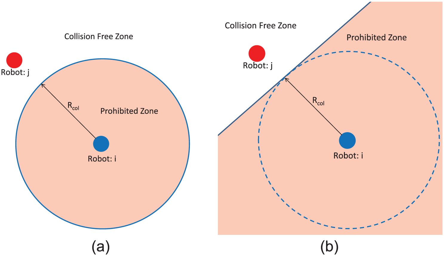In other words, the circle (2-D) or sphere (3-D) which defines the prohibited region is replaced by a line (2-D) or plane (3-D) which is tangent to the circle (2-D) or sphere (3-D) and perpendicular to the line segment connecting the nominal positions ( ${\bar{x}}_{j}$ ) of the agents. The 2-D version of this idea is shown in Figure 2.

Fig. 2.

Convexification of the 2-D collision avoidance constraint (Morgan et al., 2014). (a) Nonconvex prohibited zone. (b) Convex approximation of prohibited zone.

Figure 2(a) shows the prohibited zone for the nonconvex collision avoidance constraint. Figure 2(b) demonstrates the convex approximation of the constraint. As can be seen in Figure 2(b), the new prohibited zone includes the old prohibited zone so the convex collision avoidance constraint is a sufficient condition for the original, nonconvex constraint. Therefore, collision avoidance is still guaranteed using this approximation.

The convex approximation of the nonconvex program in Problem 4 is shown below for agent $j$ (Morgan et al., 2014).

Problem 5 (Decentralized convex program)

min_{u_{j}} \sum_{k = k_{0}}^{T - 1} ∥ u_{j} [k] ∥_{1} Δ t subject to

(32)

\begin{matrix} x_{j} [k + 1] = A_{j} [k] x_{j} [k] + B_{j} [k] u_{j} [k] + z_{j} [k], \\ k = k_{0}, \dots, T - 1 \end{matrix}

(33)

∥ u_{j} [k] ∥_{\infty} \leq U_{\max} k = k_{0}, \dots, T - 1

(34)

x_{j} [0] = x_{j, 0}

(35)

x_{j} [T] = x_{j, f}

(36)

\begin{matrix} ({\bar{x}}_{j} [k] - {\bar{x}}_{i} [k {])}^{T} G^{T} G (x_{j} [k] - {\bar{x}}_{i} [k]) \\ \geq R_{col} ∥ G ({\bar{x}}_{j} [k] - {\bar{x}}_{i} [k]) ∥_{2} \\ k = k_{0}, \dots, T, i \in {N_{[j]} \cap P_{j}} \end{matrix}

(37)

4.2. Sequential convex programming

The approximations used to make the trajectory optimization into a convex program require nominal trajectories ( ${\bar{x}}_{j}$ ) for each robot (or vehicle). Additionally, the nominal trajectories should be close to the actual state trajectories to minimize the approximation error. To ensure that the nominal vectors are good estimates of the actual state vectors, SCP is used. SCP is an iterative method, which solves a convex approximation of a nonconvex problem and uses that solution in the next iteration to convexify the problem, i.e. ${\bar{x}}_{j, w} [k] = x_{j, w - 1} [k], \forall k, w$ where $w$ is the SCP iteration. This process is repeated until the sequence of trajectories converges according to the following condition

∥ x_{j, w} [k] - x_{j, w - 1} [k] ∥_{\infty} < ε_{SCP}, \forall j, k

(38)

To enforce the collision avoidance constraints, each agent communicates its own nominal trajectory to its neighboring agents.

The SCP method is described in Method 2. First, an initial trajectory is generated for each agent without considering collision avoidance (line 2). Then, the iterative process begins with each agent solving for its optimal trajectory (line 9). Next, each agent stores the current trajectory as the nominal trajectory for the next iteration (line 12) and communicates that trajectory to its neighboring agents (line 13). Finally, the iteration is repeated until the trajectories converge and the agents are collision free (line 14).

Because the convex optimizations can be solved efficiently, the run time is now on the order of a time step or two so VSDAA and SCP can be implemented using MPC by updating the future assignments and control commands based on the current state, which may have drifted off the optimal trajectories due to unmodeled disturbances or other errors. MPC can provide some robustness to disturbances and allows the communication network to be distributed and disconnected.

4.3. Convergence of SCP

In this subsection we will show that SCP (Method 2) converges to a point, which satisfies the KKT conditions of the nonconvex optimization in Problem 4. In order to do this, we will show that the sequence of convex programs for agent $j$ converges in two different situations. First, the sequence converges when agent $j$ does not have to avoid any other agents.

Proposition 3 (Convergence without collision avoidance) If $N_{[j]} \cap P_{j} = \emptyset$ , the solution to the convex program (Problem 5) for agent $j$ is equivalent to the global minimum of the nonconvex program (Problem 4).

Proof. Since $N_{[j]} \cap P_{j} = \emptyset$ , agent $j$ does not avoid any other agents, which means that there are no collision avoidance constraints. Without collision avoidance constraints, the nonconvex program (Problem 4) and the convex program (Problem 5) are equivalent and the solution to either problem will be a global minimum to both problems.

Next, we will show that SCP converges for agent $j$ when all of the agents that agent $j$ must avoid have a fixed trajectory, i.e. their trajectories do not change from one iteration to the next. First, we establish that a solution to the convex program will always be a feasible solution to the nonconvex program. To simplify the notation in the following proofs, we introduce the following definition.

Definition 1 (CP( ${\bar{x}}_{j}$ , ${\bar{x}}_{i}$ )) We define CP( ${\bar{x}}_{j}$ , ${\bar{x}}_{i}$ ) to be the convex program in Problem 5 where the nominal trajectories ${\bar{x}}_{j}$ and ${\bar{x}}_{i}$ are used for the convexification and decoupling, respectively, of the nonconvex program in Problem 4. The sets $N_{[j]}$ and $P_{j}$ are the same as in the nonconvex program (Problem 4).

Proposition 4 (Feasible solutions) If $(x_{j, w}, u_{j, w})$ is a feasible solution to, then $(x_{j, w}, u_{j, w})$ is a feasible solution to the nonconvex program (Problem 4).

Proof. Since $(x_{j, w}, u_{j, w})$ is a solution to Problem 5, it satisfies all of the constraints of Problem 5. Except for the collision avoidance constraint (31), the constraints of the nonconvex program (27)-(30) are the same as those of the convex program (33)-(36). Additionally, $x_{j, w}$ satisfies equation (37). Therefore, the following is true for all $k = k_{0}, \dots, T$ and $i \in {N_{[j]} \cap P_{j}}$

\begin{matrix} (x_{j, w - 1} [k] - {\bar{x}}_{i} [k {])}^{T} G^{T} G (x_{j, w} [k] - {\bar{x}}_{i} [k]) \\ \geq R_{col} ∥ G (x_{j, w - 1} [k] - {\bar{x}}_{i} [k]) ∥_{2} \\ ∥ G (x_{j, w - 1} [k] - {\bar{x}}_{i} [k]) ∥_{2} ∥ G (x_{j, w} [k] - {\bar{x}}_{i} [k]) ∥_{2} \\ \geq R_{col} ∥ G (x_{j, w - 1} [k] - {\bar{x}}_{i} [k]) ∥_{2} \\ ∥ G (x_{j, w} [k] - {\bar{x}}_{i} [k]) ∥_{2} \geq R_{col} \end{matrix}

(39)

The last equation in (39) shows that $x_{j, w}$ satisfies the collision avoidance constraint in equation (31). Therefore, all of the constraints in Problem 4 are satisfied and $x_{j, w}$ is a feasible solution to Problem 4.□

The above proposition shows that any solution to the convex program is a feasible solution to the nonconvex program. Next, this fact will be used to establish that a sequence of optimal solutions exist.

Proposition 5 (Optimal sequence) Let $x_{i}$ be fixed trajectories for all $i \in {N_{[j]} \cap P_{j}}$ . If $(x_{j, w}, u_{j, w})$ is a feasible solution to or the nonconvex program (Problem 4), then has an optimal solution and $(x_{j, w}, u_{j, w})$ is a feasible solution to .

Proof. Since $(x_{j, w}, u_{j, w})$ is a solution to CP( $x_{j, w - 1}$ , ${\bar{x}}_{i}$ ) or Problem 4, it satisfies equations (33)–(36), which are the same as the constraints of CP( $x_{j, w}$ , ${\bar{x}}_{i}$ ) except for the collision avoidance constraints (37). Additionally, $x_{j, w}$ satisfies the collision avoidance constraints of CP( $x_{j, w - 1}$ , ${\bar{x}}_{i}$ ) or Problem 4. If $x_{j, w}$ satisfies the constraints of Problem 4, the first line of (40) is established, otherwise, this line is established by Proposition 4

\begin{matrix} ∥ G (x_{j, w} [k] - {\bar{x}}_{i} [k]) ∥_{2} \geq R_{col} \\ ∥ G (x_{j, w} [k] - {\bar{x}}_{i} [k]) ∥_{2}^{2} \geq \\ R_{col} ∥ G (x_{j, w} [k] - {\bar{x}}_{i} [k]) ∥_{2} \end{matrix}

(40)

\begin{matrix} (x_{j, w} [k] - {\bar{x}}_{i} [k {])}^{T} G^{T} G (x_{j, w} [k] - {\bar{x}}_{i} [k]) \geq \\ R_{col} ∥ G (x_{j, w} [k] - {\bar{x}}_{i} [k]) ∥_{2} \end{matrix}

The last equation in (40) shows that $x_{j, w}$ satisfies the collision avoidance constraints in CP( $x_{j, w}$ , ${\bar{x}}_{i}$ ). Therefore, $(x_{j, w}, u_{j, w})$ is a feasible solution to CP( $x_{j, w}$ , ${\bar{x}}_{i}$ ) and the set of feasible solutions to CP( $x_{j, w}$ , ${\bar{x}}_{i}$ ) is not empty. Additionally, this set is an intersection of half spaces and equality constraints, which results in a closed set, and equations (33)–(35) ensure that the set is bounded. Also, the cost of CP( $x_{j, w}$ , ${\bar{x}}_{i}$ ) is continuous. By the Weierstrass theorem (Jongen et al., 2004), a continuous function over a closed and bounded set achieves an optimum. Therefore, an optimal solution to CP( $x_{j, w}$ , ${\bar{x}}_{i}$ ) exists.

Proposition 5 shows that once a feasible solution to CP( $x_{j, w}$ , ${\bar{x}}_{i}$ ) exists, all of the following convex problems have an optimal solution and a sequence of optimal solutions ${x_{j, w}}$ exists. The next proposition shows that the optimality of this sequence is improving.

Proposition 6 (Decreasing cost) If $(x_{j, w}, u_{j, w})$ is the optimal solution to and $(x_{j, w - 1}, u_{j, w - 1})$ is a feasible solution to, then

J (u_{j, w}) \leq J (u_{j, w - 1})

(41)

where $J (u_{j}) = \sum_{k = k_{0}}^{T - 1} ∥ u_{j} [k] ∥_{1} Δ t$ . Additionally, if $(x_{j, w}, u_{j, w})$ is the unique optimal solution, then either $(x_{j, w}, u_{j, w}) = (x_{j, w - 1}, u_{j, w - 1})$ or

J (u_{j, w}) < J (u_{j, w - 1})

(42)

Proof. Since $(x_{j, w - 1}, u_{j, w - 1})$ is a feasible solution to CP( $x_{j, w - 2}$ , ${\bar{x}}_{i}$ ), Proposition 5 states that $(x_{j, w - 1}, u_{j, w - 1})$ is a feasible solution to CP( $x_{j, w - 1}$ , ${\bar{x}}_{i}$ ). Additionally, $(x_{j, w}, u_{j, w})$ is the optimal solution to CP( $x_{j, w - 1}$ , ${\bar{x}}_{i}$ ), which means that any $(x_{j}, u_{j})$ that is a feasible solution of CP( $x_{j, w - 1}$ , ${\bar{x}}_{i}$ ) satisfies

J (u_{j, w}) \leq J (u_{j})

(43)

Substituting $(x_{j, w - 1}, u_{j, w - 1})$ into the right hand side of the above equation establishes equation (41). If $(x_{j, w}, u_{j, w})$ is a unique optimal solution, then equation (43) has a strict inequality provided that $u_{j} \neq u_{j, w}$ . Substituting in $(x_{j, w - 1}, u_{j, w - 1})$ establishes equation (42) unless $(x_{j, w}, u_{j, w}) = (x_{j, w - 1}, u_{j, w - 1})$ .□

This proposition establishes that a sequence of optimal solutions ${x_{j, w}}$ has a nonincreasing cost and if these solutions are unique, they have a decreasing cost.

We will now use the propositions developed in this section to show that a sequence of optimal solutions exists and converges to an optimal solution of Problem 4. The following theorem establishes these claims.

Theorem 7 (Convergence of SCP) Let $x_{i}$ be fixed trajectories for all $i \in {N_{[j]} \cap P_{j}}$ . If $(x_{j, 1}, u_{j, 1})$ is a feasible solution to Problem 4, then a sequence of optimal solutions $({x_{j, w}}, {u_{j, w}})$ exists. If each optimal solution is unique, the sequence converges to $(x_{j}^{\infty}, u_{j}^{\infty})$ , which is a KKT point of Problem 4.

Proof. Since $(x_{j, 1}, u_{j, 1})$ is a feasible solution to Problem 4, it follows from Proposition 5 that CP( $x_{j, 1}$ , ${\bar{x}}_{i}$ ) has an optimal solution, which we call $(x_{j, 2}, u_{j, 2})$ . Applying Proposition 5 again results in an optimal solution to CP( $x_{j, 2}$ , ${\bar{x}}_{i}$ ) defined to be $(x_{j, 3}, u_{j, 3})$ . Repeating this process yields the optimal solution sequence $({x_{j, w}}, {u_{j, w}})$ . Since the optimal solutions are unique, applying Proposition 6 to this sequence yields the following condition for all $w$

J (u_{j, w}) < J (u_{j, w - 1})

(44)

Since every solution in the sequence $({x_{j, w}}, {u_{j, w}})$ satisfies equations (33)–(36), which form a closed and bounded set, there is an infinite subsequence $({x_{j, w_{i}}}, {u_{j, w_{i}}})$ that converges. Let the convergence point be called $(x_{j}^{\infty}, u_{j}^{\infty})$ . Because the cost function ( $J (u$ )) is continuous, $J (u_{j, w_{i}})$ converges to $J (u_{j}^{\infty})$ . Additionally, the cost function is decreasing as seen in equation (44). Therefore, the cost function of the entire sequence ( $J (u_{j, w})$ ) converges to $J (u_{j}^{\infty})$ . In the remainder of this proof, → will be used to denote that the sequence on its left converges to value on its right.

We define a mapping $M (x_{j})$ that represents solving CP( $x_{j}$ , ${\bar{x}}_{i}$ ). The mapping $M$ has a fixed point at $x_{j}^{\infty}$ . We will show that this is true by contradiction. Assume that $(x_{j}^{\infty + 1}, u_{j}^{\infty + 1}) = M (x_{j}^{\infty})$ and $(x_{j}^{\infty + 1}, u_{j}^{\infty + 1}) \neq (x_{j}^{\infty}, u_{j}^{\infty})$ . In this case, $J (u_{j, \infty + 1}) < J (u_{j}^{\infty}$ ). However, ${J (u_{j, w})} \to J (u_{j}^{\infty})$ so we have, for $w > \infty + 1$ , that $J (u_{j, w}) < J (u_{j}^{\infty})$ and ${J (u_{j, w})} \to J (u_{j}^{\infty})$ , which is a contradiction. Therefore, $(x_{j}^{\infty}, u_{j}^{\infty}) = M (x_{j}^{\infty})$ .

Additionally, the mapping $M (x_{j})$ is equivalent to solving the KKT conditions of CP( $x_{j}$ , ${\bar{x}}_{i}$ ), which are continuous with respect to $x_{j}$ . Therefore, the mapping $M$ is continuous. Since the subsequence $({x_{j, w_{i}}}, {u_{j, w_{i}}}) \to (x_{j}^{\infty}, u_{j}^{\infty})$ and $M$ is continuous, the following is true

{M (x_{j, w_{i}})} \to M (x_{j}^{\infty})

(45)

Additionally, $x_{j}^{\infty}$ is a fixed point and $x_{j, w_{i} + 1} = M (x_{j, w_{i}})$ . Therefore

{x_{j, w_{i} + 1}} \to x_{j}^{\infty}

(46)

This process can be repeated to show that all subsequences ${x_{j, w_{i} + n}}$ converge to $x_{j}^{\infty}$ . Therefore, the sequence ${x_{j, w}}$ converges to $x_{j}^{\infty}$ .

Finally, we will show that $(x_{j}^{\infty}, u_{j}^{\infty})$ is a KKT point of Problem 4. Since $x_{j}^{\infty}$ is a fixed point of $M$ , it is a solution to CP( $x_{j}^{\infty}$ , ${\bar{x}}_{i}$ ) and from Proposition 4, it is a feasible solution to Problem 4. Additionally, Problem 5 is convex so any solution to this problem is a KKT point ( $x_{j}^{*}$ ) and satisfies stationarity (47), complementary slackness (48), and dual feasibility (49)–(50)

\begin{matrix} 0 = \partial J (u_{j}^{*}) + (λ_{1}^{*})^{T} \partial g_{1} (x_{j}^{*}, u_{j}^{*}) + (λ_{2}^{*})^{T} \partial g_{2} (x_{j}^{*}, u_{j}^{*}) \\ + (λ_{eq}^{*})^{T} \partial g_{eq} (x_{j}^{*}, u_{j}^{*}) \end{matrix}

(47)

0 = (λ_{1}^{*})^{T} g_{1} (x_{j}^{*}, u_{j}^{*}) + (λ_{2}^{*})^{T} g_{2} (x_{j}^{*}, u_{j}^{*})

(48)

λ_{1}^{*} \geq 0

(49)

λ_{2}^{*} \geq 0

(50)

where

g_{1} (x_{j}, u_{j}) = ∥ u_{j} [k] ∥_{\infty} - U_{\max}, \forall k = k_{0}, \dots, T

(51)

\begin{matrix} g_{2} (x_{j}, u_{j}) = R_{col} ∥ G (x_{j}^{*} [k] - {\bar{x}}_{i}) ∥_{2} - (x_{j}^{*} [k] - {\bar{x}}_{i})^{T} G^{T} \\ G (x_{j} [k] - {\bar{x}}_{i}), \forall k = k_{0}, \dots, T \end{matrix}

(52)

\begin{matrix} g_{eq} (x_{j}, u_{j}) = \\ [\begin{matrix} x_{j} [k + 1] - A_{j} [k] x_{j} [k] - B_{j} [k] u_{j} [k] - s_{j} [k], \forall k = k_{0}, \dots, T - 1 \\ x_{j} [0] - x_{j, 0} \\ x_{j} [T] - x_{j, f} \end{matrix}] \end{matrix}

(53)

We note that the cost $J$ and the constraints in $g_{1}$ and $g_{eq}$ are the same in both Problems 4 and 5. Therefore, we will only substitute equation (52) for $g_{2}$ in the KKT conditions. Since $(x_{j}^{\infty}, u_{j}^{\infty})$ is a KKT point of CP( $x_{j}^{\infty}$ , ${\bar{x}}_{i}$ ), the following equations hold

\begin{matrix} 0 = \partial J (u_{j}^{\infty}) + (λ_{1}^{\infty})^{T} \partial g_{1} (x_{j}^{\infty}, u_{j}^{\infty}) - (λ_{2}^{\infty})^{T} \\ (x_{j}^{\infty} [k] - {\bar{x}}_{i})^{T} G^{T} G \\ + (λ_{eq}^{\infty})^{T} \partial g_{eq} (x_{j}^{\infty}, u_{j}^{\infty}) \end{matrix}

(54)

\begin{matrix} 0 = (λ_{1}^{\infty})^{T} g_{1} (x_{j}^{\infty}, u_{j}^{\infty}) + (λ_{2}^{\infty})^{T} (R_{col} - ∥ G (x_{j}^{\infty} [k] - {\bar{x}}_{i}) ∥_{2}) \\ ∥ G (x_{j}^{\infty} [k] - {\bar{x}}_{i}) ∥_{2} \end{matrix}

(55)

λ_{1}^{\infty} \geq 0

(56)

λ_{2}^{\infty} \geq 0

(57)

Now let $λ_{1}^{*} = λ_{1}^{\infty}$ , $λ_{2}^{*} = λ_{2}^{\infty} ∥ G (x_{j}^{\infty} [k] - {\bar{x}}_{i}) ∥_{2}$ , and $λ_{eq}^{*} = λ_{eq}^{\infty}$ , where $(λ_{1}^{\infty}, λ_{2}^{\infty}, λ_{eq}^{\infty})$ are the KKT multipliers that satisfy the KKT conditions for the convex program. Equations (54)–(57) become the KKT conditions for Problem 4.

\begin{matrix} 0 = \partial J (u_{j}^{\infty}) + (λ_{1}^{*})^{T} \partial g_{1} (x_{j}^{\infty}, u_{j}^{\infty}) \\ - (λ_{2}^{*})^{T} \frac{{(x_{j}^{\infty} [k] - {\bar{x}}_{i})}^{T} G^{T} G}{∥ G (x_{j}^{\infty} [k] - {\bar{x}}_{i}) ∥_{2}} \\ + (λ_{eq}^{*})^{T} \partial g_{eq} (x_{j}^{\infty}, u_{j}^{\infty}) \end{matrix}

(58)

0 = (λ_{1}^{*})^{T} g_{1} (x_{j}^{\infty}, u_{j}^{\infty}) + (λ_{2}^{*})^{T} (R_{col} - ∥ G (x_{j}^{\infty} [k] - {\bar{x}}_{i}) ∥_{2})

(59)

λ_{1}^{*} \geq 0

(60)

λ_{2}^{*} \geq 0

(61)

Therefore, $(x_{j}^{\infty}, u_{j}^{\infty})$ satisfies the KKT conditions for the nonconvex program (Problem 4) with lagrange multipliers, $(λ_{1}^{*}, λ_{2}^{*}, λ_{eq}^{*})$ .

Proposition 3 and Theorem 7 show that the SCP algorithm (Algorithm 2) applied to the convex program (Problem 5) converges to a trajectory that satisfies the KKT conditions of the nonconvex program (Problem 4). Proposition 3 applies when there are no collision avoidance constraints ( $N_{[j]} \cap P_{j} = \emptyset$ ) and Theorem 7 applies when the agents that need to be avoided have a fixed trajectory ( $x_{i, w} = x_{i}^{\infty}, \forall w, \forall i \in N_{[j]} \cap P_{j}$ ). In order to guarantee that the SCP algorithm for every agent converges, a priority value ( $ρ_{j}$ ) is defined for each agent and is used to construct $P_{j}$ .

Theorem 8 (Convergence of all agents) Let each agent $j$ have a priority value $ρ_{j}$ such that $ρ_{i} \neq ρ_{j}$ for any $i \neq j$ . Define the priority set as follows

P_{j} = {i | ρ_{i} < ρ_{j}}

(62)

If there is a feasible solution to Problem 4 for each agent and $N_{[j]} = 1, \dots, N$ , all of the agents will converge to a KKT solution of Problem 4 and no collisions occur.

Proof. Since $ρ_{i} \neq ρ_{j}$ for any $i \neq j$ , there exists an agent $j_{1}$ such that $ρ_{j_{1}} < ρ_{j}$ for all $j \neq j_{1}$ . This will result in $P_{j_{1}} = \emptyset$ . Using Proposition 3, agent $j_{1}$ converges to a solution that is a global minimum of Problem 4 and therefore, satisfies the KKT conditions. This solution is defined as $x_{j_{1}}^{*}$ .

Now there exists an agent $j_{2}$ such that $ρ_{j_{2}} < ρ_{j}$ for all $j \neq {j_{1}, j_{2}}$ and $ρ_{j_{1}} < ρ_{j_{2}}$ . This implies that $P_{j_{2}} = j_{1}$ . Now, Theorem 7 can be applied, using the assumption that there is a feasible solution and the fact that $x_{j_{1}}^{*}$ is fixed, to show that the SCP algorithm for agent $j_{2}$ converges to a solution ( $x_{j_{2}}^{*}$ ) that is a KKT point of Problem 4. This step can be repeated for all of the remaining agents to show that every agent’s trajectory converges to a KKT point.

Additionally, since $i \in P_{j}$ if and only if $ρ_{i} < ρ_{j}$ we can state that exactly one of the following statements is true for all pairs $(i, j)$ : $i \in P_{j}$ or $j \in P_{i}$ . Since either $i$ or $j$ will avoid the other one, the collision is accounted for in the optimizations. Since this is true for all agent pairs, every possible collision is considered in the optimizations so no collisions will occur.

Remark 7 (Priority value ( $ρ_{j}$ )) The priority values ( $ρ_{j}$ ) described in Theorem 8 should be defined by a physical parameter that reflects the ability of each agent to avoid other agents. The most obvious choice for this value is the fuel/battery remaining for each agent. Using this quantity, the agent with more fuel/battery remaining would avoid the collision. Also, the priority values should remain constant throughout a complete reconfiguration for Theorems 7 and 8 to hold. However, they can change from one reconfiguration formation shape to the next.

Remark 8 (SCP computational complexity) The number of robots affects the number of collision avoidance constraints. When the swarm has all-to-all communication, the number of constraints scales linearly with the number of robots so the complexity is $O (N)$ . However, when robots can only communicate with neighboring robots, the number of constraints scales linearly with the density of robots so the complexity is $O (N (R_{comm} / L)^{d})$ where $d$ is the dimension of the physical space and $L$ is the size of the physical space in any dimension.

5. Swarm assignment and trajectory optimization

In this section, MPC is used to implement the VSDAA and SCP methods in real time, creating the swarm assignment and trajectory optimization (SATO) algorithm. Additionally, the communication requirement in the swarm is reduced so that the network does not need to be centralized or even connected for the algorithm to work. MPC uses a receding horizon to update the optimal assignments and trajectories based on the current state information. Once an optimal control sequence or optimal assignment is calculated, those values are used until updated values are calculated.

5.1. Model predictive control formulation

SATO updates the state ( $x_{j, k_{0}}$ ) and time ( $k_{0}$ ) and uses this information as the initial conditions in the optimization. Additionally, a receding horizon, which is $T_{H}$ time steps long, is used to reduce the size of the optimizations so that they can be run more frequently. We will consider communication networks that are distributed and disconnected. With these ideas in mind, each agent will only consider collision avoidance with their neighboring agents and only for the length of the horizon. This allows us to reduce the size of the optimizations without hindering the safety of the agents by considering future collision avoidance in future optimizations. To incorporate these ideas into SATO we modify the collision avoidance constraint in equation (37) as follows

\begin{matrix} ({\bar{x}}_{j} [k] - {\bar{x}}_{i} [k {])}^{T} G^{T} G (x_{j} [k] - {\bar{x}}_{i} [k]) \\ \geq R_{col} ∥ G ({\bar{x}}_{j} [k] - {\bar{x}}_{i} [k]) ∥_{2} \\ k = k_{0}, \dots, min {k_{0} + T_{H}, T}, i \in N_{[j]} \cap P_{j} \end{matrix}

(63)

where

N_{[j]} = {i | ∥ x_{j} [k_{0}] - x_{i} [k_{0}] ∥_{2} \leq R_{comm}}

(64)

and $R_{comm}$ is the communication radius of each agent.

Since we are only considering collisions between neighboring agents, it is important to guarantee that no agents can start in positions where they cannot communicate and end up colliding before a new trajectory is generated. To do this, an artificial velocity constraint is introduced so that a bound can be placed on the distance two agents can move relative to each other in a limited amount of time. This constraint is shown below

∥ H x_{j} [k] ∥_{2} \leq V_{\max} k = k_{0}, \dots, T

(65)

where $H = [0_{3 \times 3} I_{3 \times 3}]$ .

Next, we define two modifications of Problem 5. The first modification is used in SATO to estimate the costs used in VSDAA. The problem is defined as follows.

Problem 6 (Auction cost)

\begin{matrix} min_{u_{j}} \sum_{k = k_{0}}^{T - 1} ∥ u_{j} [k] ∥_{1} Δ t subject to {, (9) (11), (13), (65)}, \\ and x_{j} [T] = X_{f} (j) \end{matrix}

(66)

It is important to note that this problem does not include collision avoidance. This is due to the fact that collisions are highly dependent on the assignment, which has not been determined when this problem is used. Additionally, the number of collisions will generally be small for the optimal assignment so excluding them should not have a large effect on the cost.

The other modified problem that will be introduced will be used when SATO uses SCP. This problem is defined below.

Problem 7 (Limited horizon SCP)

\begin{matrix} min_{u_{j}} \sum_{k = k_{0}}^{T - 1} ∥ u_{j} [k] ∥_{1} Δ t subject to \\ {(9), (11), (13), (17), (63), (65)} \end{matrix}

(67)

This problem uses the new collision avoidance constraint, which considers collisions only in the short term, with respect to both position and time.

SATO is described in Method 3. First, the auction costs are generated for each agent going to each target position (line 5). Then, VSDAA is used to compute the optimal assignment (line 9). Next, SCP is used to generate the optimal trajectory and corresponding control sequence (line 14). Finally, the optimal control sequence is applied until a new optimal control is generated (line 16). The current time and state are then updated and the process is repeated until the terminal time is reached.

Method 3 Swarm assignment and trajectory optimization (SATO).
1: $k_{0} = 0$
2:while $k_{0} \leq T$ do
3: for all $i = 1, \dots, N$ (parallel) do
4: for all $j = 1, \dots, M$ do
5: Solve Problem 6 using SCP (Method 2)
6: $c^{i} (j) =$ cost of optimal solution to Problem 6
7: end for
8: end for
9: Solve Problem 2 using VSDAA (Method 1)
10: $x_{j, f} =$ solution to Problem 2, $\forall j$
11: if # of bids has changed then
12: $k_{0} = 0$
13: end if
14: Solve Problem 7 using SCP (Method 2)
15: $u_{j} [k] =$ control solution to Problem 7, $\forall j$ , $k = k_{0} \dots k_{0} + T_{H} - 1$
16: Apply $u_{j} [k]$ for $k = k_{0} \dots k_{0} + T_{H} - 1$
17: Update $k_{0}$ and $x_{j, k_{0}}$ to current time
18:end while

After the optimal assignment is computed, the algorithm checks to see if the number of targets that have been bid upon has changed from the previous iteration. If the number of bids has changed, that means that the number of agents in the communication network has changed. This can result in significantly different assignments due to new information about other agents. To prevent the new assignment from creating an infeasible trajectory optimization, the current time or the terminal time is reset to give each agent enough time to go to its new target.

Remark 9 (Extend the terminal time) If the optimization is infeasible due to maximum velocity or control constraints, the final time $T$ can be extended to $T + n_{t} Δ T$ , where the integer value $n_{t}$ increases from 1 until the optimization becomes feasible. Then the agents can communicate the new terminal time. The ability to bound the terminal time is largely dependent on the problem formulation, i.e. dynamics, cost function, constraints. A bound on maximum terminal time could be calculated by upper bounding the distance between agents and targets, and determining the time to cover that distance given the velocity and control constraints.

5.2. Disconnected communication network

A typical auction algorithm cannot achieve a proper assignment when the communication network is disconnected. Without the assumption of a connected network, the proof of Proposition 2 breaks down. In fact, we cannot even guarantee that every target has at most one agent assigned to it since the bid of one agent cannot reach all of the other agents. However, we will show that using the MPC implementation contained in SATO allows the assignment algorithm to achieve an optimal assignment. First, we develop a condition that guarantees that two robots, which cannot communicate, will not collide before the end of the MPC horizon.

Proposition 9 (Detectable collisions (Morgan et al., 2014)). If two agents cannot communicate, they will not collide before the end of the current horizon if

R_{comm} \geq 2 V_{\max} T_{H} Δ t + R_{col} and Δ t V_{\max} < R_{col}

(68)

Proof. The amount of time in the current horizon is the number of time steps ( $T_{H}$ ) multiplied by the time step size ( $Δ t$ ). Since the relative velocity is bounded by $2 V_{\max}$ , the maximum change in the relative distance between two agents is $2 V_{\max} T_{H} Δ t$ . Therefore, this distance must be less than the difference between the communication radius ( $R_{comm}$ ) and the collision radius ( $R_{col}$ ). This establishes the first inequality of equation (68). Also, the second condition in equation (68) ensures collision-free motion during two consecutive time steps $k$ and $k + 1$ .□

This condition guarantees that any agent that could potentially cause a collision before the end of the MPC horizon is detected and therefore considered in the optimization. An illustration of a pair of robots that violate this condition is shown in Figure 3(a). Furthermore, the drift of each agent off of its desired trajectory can be bounded based on the robust nonlinear tracking control law design given in Section 7 and measurement/modeling errors. 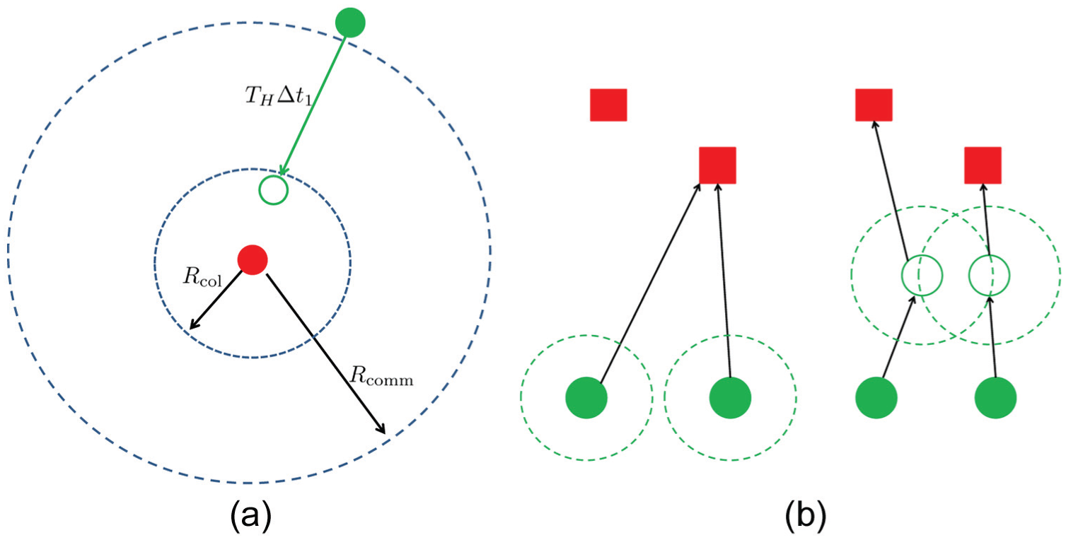This error bound can then be used to increase the collision radius ( $R_{col}$ ), see Morgan et al. (2014) for details.

Fig. 3.

Visualization of an undetectable collision and an assignment conflict being resolved. (a) Illustration of an undetectable collision. (b) Resolution of an assignment conflict.

While Proposition 9 was created in our prior work (Morgan et al., 2014) with respect to trajectory optimizations, it also applies to the assignment part of SATO. This condition guarantees that before two agents, which are in disconnected communication networks and assigned to the same target, collide, a new assignment will be run with those agents being able to communicate. At this point, VSDAA guarantees that they will be assigned to different targets and that within their connected network, the assignment will be optimal. This idea allows each connected network to perform its own assignment, which will be optimal. If there is no conflict between the networks, no two agents in different networks have bid on the same target so all of the current bids are the highest bids and the solution is optimal. On the other hand, if there is a conflict, the conflicting agents will go to the same target resulting in them being able to communicate before they collide. At this point, they are on the same communication network and will resolve the conflict. Figure 3(b) shows an assignment conflict being resolved once the agents can communicate. When the agents are at the solid circles, they cannot communicate and they choose the same target. However, as they move towards the target, they reach the open circles and become connected. At this point, they will be assigned to different target, which resolves the conflict.

Although each individual conflict will eventually be resolved, there is no guarantee that the new assignment does not cause a conflict with another robot that is outside of the communication radius. Once again, this conflict will be resolved, but the resolution could cause another conflict. This process will not repeat indefinitely due to the bound on the number of bids that can be placed in the auction algorithm, but an individual vehicle can run out of fuel before all of the conflicts are resolved. The most likely scenario where this can occur is when one vehicle is moving back and forth between two disconnected networks. In this case, a single vehicle essentially becomes a messenger between the two networks and must physically move between the networks to transfer the bids. This vehicle runs the risk of using all of its fuel before an optimal assignment is achieved. Additionally, if the maximum available fuel is used to set the cost of unreachable targets to infinity, the problem can become infeasible since some of the vehicles are using fuel to move between the networks.

This problem is more likely to occur when the communication network is disconnected and targets are far apart from one another. The simplest solution is to ensure that the targets are sufficiently close together so that the target swarm has a connected communication network. The other solution is to decrease the probability that the communication network can become disconnected. The probability of having a connected communication network is dependent on the number of agents and the size of the communication radius relative to the volume in which the robots are located. The following equation (Corollary 6 in Yu et al. (2015)) determines the number of agents required to achieve a certain probability of connectedness

N \geq ⌈ \frac{\sqrt{5}}{R_{comm}} ⌉^{2} \log [\frac{1}{1 - p} (\frac{1}{2} {⌈ \frac{\sqrt{5}}{R_{comm}} ⌉}^{2} + ⌈ \frac{\sqrt{5}}{R_{comm}}]) ⌉

(69)

where $N$ is the number of randomly distributed agents with communication radius ( $R_{comm}$ ) required to achieve a connected network with probability $p$ in a 2-D unit square. While this bound applies specifically to a 2-D unit square, the general trends are the same: having more agents and larger communication radii increases the probability of a connected network.

6. Simulation results

In this section, we apply SATO to swarms in two different dynamic environments. First, we apply SATO to a 2-D environment with double integrator dynamics. This simulation represents the most common problem in the swarm robotics community and can be used to compare SATO to the existing algorithms in that field. In the second simulation, we apply SATO to a swarm of spacecraft in 3-D using the high-fidelity dynamic models of spacecraft in low Earth orbit. This simulation shows that SATO can be used even when the dynamics are nonlinear and state dependent.

6.1. Simulation with 2-D double integrator dynamics

In the 2-D double integrator simulation, a swarm of 123 agents is randomly initialized and undergoes four reconfigurations forming the letters ‘U’, ‘I’, ‘U’, and ‘C’, respectively. As discussed in Remark 4, we use the squared distance between the initial and the terminal points as the assignment cost function. During the first reconfiguration, the communication network is initially disconnected since the swarm is randomly distributed. As the agents begin to form the ‘U’, they move closer to each other and the communication network becomes more connected. As the agents become more connected conflicting assignments are resolved and the swarm achieves the desired shape. After the second reconfiguration (‘I’ shape), a significant number of agents are lost causing the communication network to become disconnected. As the agents reconfigure from ‘I’ to ‘U’, they still believe there are 123 agents in the swarm, which results in some holes in the target shape. However, after completing the ‘U’, the agents adjust the number of targets in the assignment based on the number of bids they received while reconfiguring from ‘I’ to ‘U’. This is seen when the swarm successfully achieves a ‘C’ without any holes. The results of the simulation are shown in Figures 4 and 5.

Fig. 4.

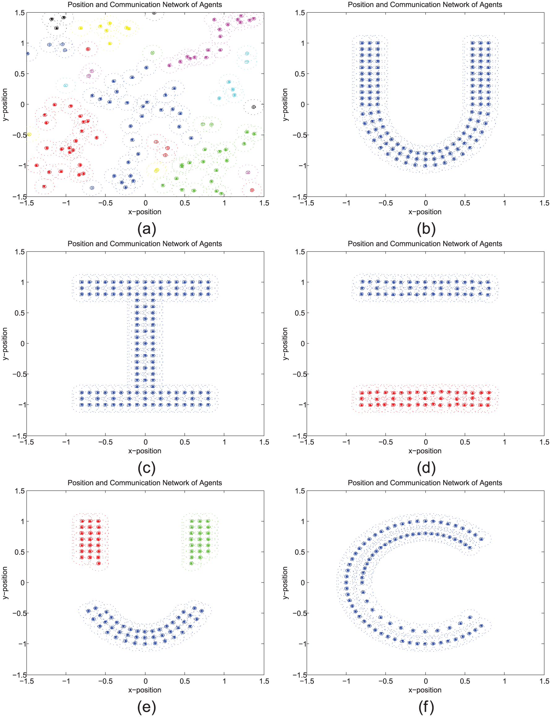
Various time instances in the UIUC reconfiguration simulation. See Extension 1. (a) Initial swarm (k = 0). (b) ‘U’-shaped swarm (k = 34). (c) ‘I’-shaped swarm (k = 56). (d) ‘I’-shaped swarm after loss of agents (k = 57). (e) ‘U’-shaped swarm (k = 76). (f) ‘C’-shaped swarm (k = 104).

Fig. 5.

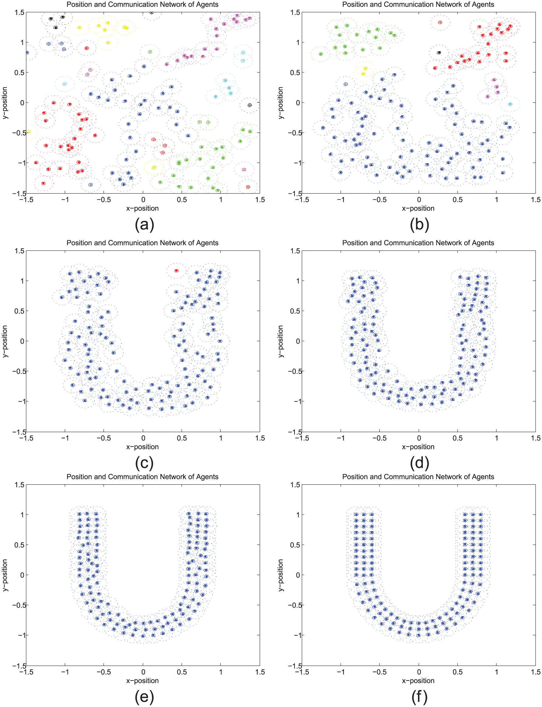
Various time instances in the reconfiguration simulation from a random swarm to a ‘U’ shape. (a) k = 0. (b) k = 7. (c) k = 14. (d) k = 21. (e) k = 28. (f) k = 34. See Extension 1.

Figure 4 shows the swarm shape after each reconfiguration. Each agent is shown with a given marker shape and color, which denotes its communication network. Agents with the same shape and color are connected and agents with different shapes or colors are not connected. Additionally, the dotted circle around each agent represents half of the agents communication radius. Therefore, any agents whose communication circles touch can communicate with each other.

Figure 4(a) shows the initial swarm distribution and the disconnected communication networks due to the random distribution. Figure 4(b) shows the ‘U’-shaped swarm after the first reconfiguration. In Figure 4(c), the ‘I’-shaped swarm that occurs after the second reconfiguration is shown. Figure 4(d) shows the ‘I’-shaped formation after many of the agents have been lost. This loss of agents results in two disconnected groups of agents (red and blue). In Figure 4(e), the swarm forms a ‘U’ shape but due to the loss of agents there are holes in the formation. Finally, Figure 4(f) shows the ‘C’ shape swarm after the final reconfiguration. Although the ‘C’ is not complete due to the loss of agents, VSDAA adjusts the number of targets in the assignment so that there are no large gaps in the desired shape.

Figure 5 shows several time instances of the first reconfiguration. In this reconfiguration, a random swarm transforms into a ‘U’ shape. As with Figure 4, the connected agents are shown with the same color and shape while the dotted circle represents half of the communication radius. Figure 5 shows the evolution of the communication network as the swarm converges to its desired shape.

Figure 5(a) shows the initial swarm with many disconnected communication networks. In Figure 5(b), over half of the swarm is connected (blue) and the agents are roughly starting to form a ‘U’. In Figure 5(c), all but one of the agents are connected so the assignment is nearly complete and the agents are moving towards their targets. Figures 5(d)–(f) show the movement of the swarm once the agents are all connected and the assignment is complete. These figures show the trajectory optimization part of SATO as the agents reach their desired positions in Figure 5(f).

6.2. Simulation with 3-D relative orbital dynamics with $J_{2}$

The objective of this simulation study is to show that the SATO algorithm can effectively handle complex dynamic models defined for 3-D motions. In the 3-D spacecraft swarm simulation, the agents are randomly initialized and reconfigured to form a circle. In this simulation, the relative orbital dynamics with $J_{2}$ (Morgan et al., 2012) are used as the dynamics constraints when SATO calls Problems 6 and 7. The initial and terminal positions are random and circular, respectively, and the velocities are generated using $J_{2}$ -invariant conditions from our prior work (Morgan et al., 2012). Additionally, the random initial positions and the target circle are both located in the $x$ (radial)- $y$ (alongtrack) plane, but the trajectories are allowed to move out of plane. We place the initial and terminal conditions with this constraint so that the plots can be more easily interpreted. However, SATO is equally effective when the initial and terminal positions also have out-of-plane components.

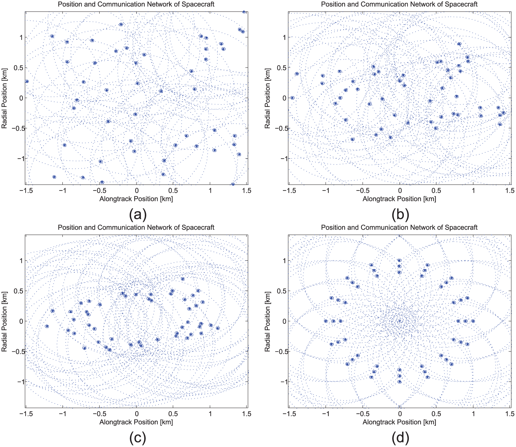
Figure 6 shows the reconfiguration of a swarm of 48 spacecraft from a random distribution to a circular formation. The reference orbit used for this simulation is a circular orbit with a semimajor axis of 6878 km, and an inclination of 45 degrees. The reconfiguration occurs in a quarter of an orbit, which is equal to about 24 minutes. The time step size ( $Δ t$ ) is one minute, the communication radius ( $R_{comm}$ ) is 2 km, and the collision radius ( $R_{col}$ ) is 50 m.

Fig. 6.

Various time instances in the reconfiguration simulation of a swarm of spacecraft in the LVLH frame. The out-of-plane ( $z$ ) motion is not shown in this figure. (a) k = 0. (b) k = 8. (c) k = 16. (d) k = 24.

Figure 6(a) shows the initial swarm distribution where the spacecraft are randomly distributed. Figures 6(b), (c) and (d) show the reconfiguration after 8, 16, and 24 minutes, respectively. In Figure 6(d), the swarm has achieved its desired formation of a circle. The results of this simulation show that SATO still achieves the optimal assignment and trajectory generation when the dynamics are as complicated as the relative dynamics of a spacecraft in low Earth orbit.

7. Hardware experimental results using nonlinear tracking controller

We first describe the position controller and the nonlinear attitude tracking controller that are used to track the desired position trajectories computed by SATO. The experimental results from flight tests are presented in Section 7.3. The algorithm was tested on our formation flying testbed at the University of Illinois at Urbana-Champaign. The experimental setup is composed of sixteen VICON motion capture cameras, the communication dongles for sending signals to the agents and a single computer for implementing the flight control algorithms. The computer uses a 3.4 GHz Intel Core i7 chip with 12 GB of DDR3 RAM and runs on Windows 8. The communication dongle used is a Crayradio 2.4GHz radio USB dongle which connects to the computer via a USB hub. Each dongle communicates with one quadrotor at a data rate of 250Kbps. The entire software back-end (except the motion capture system) was developed in-house (in Python 2.7) and integrates the path planner, controller, motion capture system, and radio communication into a single package. The quadrotor vehicle used for the experiments are called ‘Crazyflies’, sold by the company Bitcraze, and can be obtained commercially (see Figure 7). This platform is open-source which provides us with access to the onboard attitude sensors and actuators, hence allowing us to design our own flight control strategies for the quadrotor.

Fig. 7.

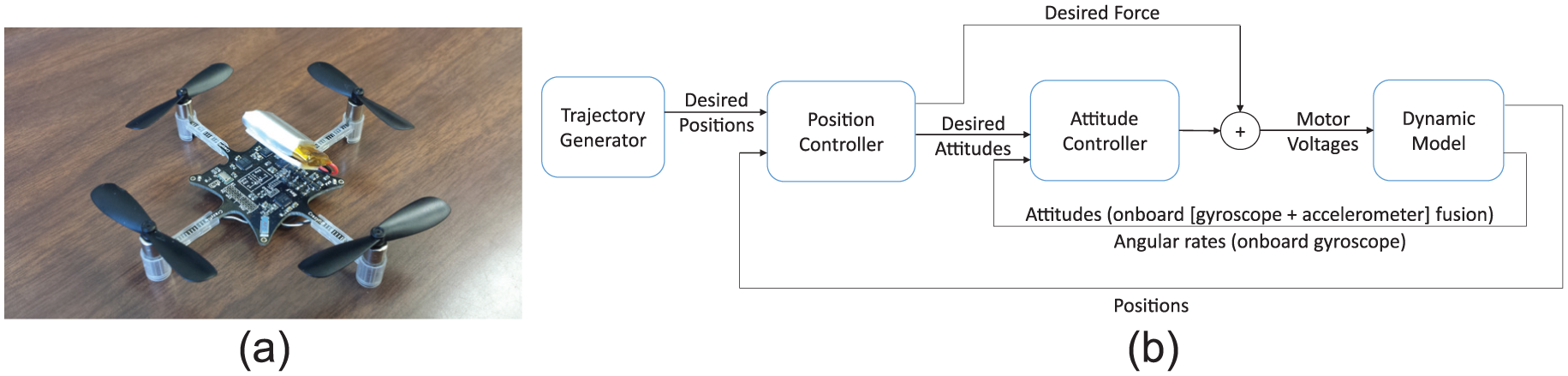
The position controller takes the current position and desired positions to generate the total desired force and the attitude commands which are tracked by the nonlinear attitude controller (71). (a) Crazyflie quadrotor. (b) Block diagram of quadrotor control.

7.1. Robust nonlinear attitude tracking control

The control law is broken down into two parts, namely: the feedback attitude control loop (inner loop) and the feedback position control loop (outer loop), as shown in Figure 7. While there have been a lot of controllers designed for quadcopters, many of them tend to linearize the dynamic model about hover or some other points and try to apply a controller on the linearized model. Even though this might be good for slow and gradual movements, it is not ideal for demanding trajectories and aggressive maneuvers. The nonlinear flight control law given in this section utilizes the full dynamic model of the quadrotor while being able to guarantee global exponential stability and bounded tracking errors with respect to bounded disturbance. This stability result allows us to tightly bound and control the size of the trajectory error for collision-free motion planning. The attitude dynamics and the corresponding kinematics equation of a rigid body are given as

J_{tot} \overset{\cdot}{ω} = (J_{tot} ω) ω + u + d_{ext}, \overset{\cdot}{q} = Z (q) ω

(70)

where $q$ is a vector of three-dimensional attitude representation (e.g. Euler angles, classical Rodrigues parameters, first three elements of quaternions, or modified Rodrigues parameters) with the appropriate definition of $Z (q) \in ℝ^{3 \times 3}$ . Also, $J_{tot}$ is the inertia matrix, $ω$ is the angular rate of the body frame with respect to the inertial frame, the vector $u = (u_{x}, u_{y}, u_{z})^{T}$ is the control torque in the body axis, and $d_{ext}$ denotes the external disturbance torque.

The following robust nonlinear tracking control law for the attitude dynamics (70) is used

\begin{matrix} u = J_{tot} {\overset{\cdot}{ω}}_{r} - (J_{tot} ω) ω_{r} - K (\overset{\cdot}{ω} - {\overset{\cdot}{ω}}_{r}) \\ ω_{r} = Z^{- 1} (q) q_{d} (t) + Z^{- 1} (q) Λ (q_{d} (t) - q) \end{matrix}

(71)

where the positive-definite matrix $K \in ℝ^{3 \times 3}$ is the feedback gain, $Λ \in ℝ^{3 \times 3}$ is a positive-definite matrix, and $q_{d} (t)$ is the time-varying desired (reference) trajectory. Note that $(J_{tot} ω) ω$ in the attitude dynamics (70) is not canceled exactly in order to reduce the effect of $(Δ J_{tot} ω) ω$ with an error from an estimated inertia matrix, $Δ J_{tot}$ .

The stability proof of equation (71), obtained by following the standard setup detailed in our prior work (Bandyopadhyay et al., 2016; Chung et al., 2013), indicates that all system trajectories converge exponentially fast to a single trajectory regardless of initial conditions with a rate given by $λ_{conv, robust} = \frac{λ_{min} (K)}{λ_{max} (J_{tot})},$ where $λ_{min} (\cdot)$ and $λ_{max} (\cdot)$ are the smallest and the largest eigenvalues respectively. Then the smallest path integral $R (t) = \int_{q_{d}}^{q} ∥ δ y ∥_{2}$ exponentially converges to the following error ball (Chung et al., 2013)

lim_{t \to \infty} R (t) \leq sup_{t} \frac{λ_{max} (J_{tot}) ∥ d {(t)}_{ext} ∥_{2}}{λ_{min} (Λ) λ_{min} (K) λ_{min} (J_{tot})} .

(72)

This ensures that the speed of convergence to any desired time-varying trajectory $q_{d} (t)$ is exponentially fast and that the controller can perform agile maneuvers starting from any initial condition with a predicted uncertainty bound. Note that the system with bounded disturbance $d_{ext}$ is also input-to-state stable (ISS) and finite-gain $L_{p}$ stable because of the global exponential stability of the unperturbed system.

If the constant bias term in $d (t)_{ext}$ is larger than the time-varying term, the advantage of equation (71) is its straightforward extension to an integral control law: $u = J_{tot} {\overset{\cdot}{ω}}_{r} - (J_{tot} ω) ω_{r} - K (\overset{\cdot}{ω} - {\overset{\cdot}{ω}}_{r}) - \int_{0}^{t} K_{I} (ω - ω_{r}) dt$ , whose stability analysis is detailed in Bandyopadhyay et al. (2016). Now that the attitude of the quadrotor can be commanded, the inner loop of Figure 7 is complete. The next step of the controller design is to develop the outer control loop of Figure 7, i.e. the position controller.

7.2. Position tracking controller

The position control law forms the outer-loop, which generates the desired attitude trajectory $q_{d} (t)$ for the attitude tracking controller presented in Section 7.1 as a function of the position errors ( $x$ - $x_{d}$ ). The desired vehicle trajectory $x_{d}$ and the estimated vehicle position $x$ are computed in the local reference frame (e.g. local obstacle map) that is evolving in the absence of a global map and $x_{d}$ is provided by the algorithms presented in Section 5. We used Euler angles for $q$ in our experiments.

The translational motion along the three axes can be given as

m \overset{\cdot\cdot}{x} = \bar{X}, m \overset{\cdot\cdot}{y} = \bar{Y}, m \overset{\cdot\cdot}{z} = - mg + \bar{Z}

(73)

where $\bar{X} = F (\cos ψ \cos ϕ \sin θ + \sin ψ \sin ϕ)$ , $\bar{Y} = F$ $(\sin ψ \cos ϕ \sin θ - \cos ψ \sin ϕ)$ , $\bar{Z} = F \cos ϕ \cos θ$ , $g$ is the acceleration due to gravity, and $m$ is the mass of the quadrotor. Also, ( $ϕ$ , $θ$ , $ψ$ ) are the Euler angles of the quadrotor and $F$ is the total force generated by the quadrotor. In order to control the position of the quadrotor, a PID controller to track the desired position trajectory along each of the three axes is sufficient (e.g. $\bar{Z} = m (g + {\overset{\cdot\cdot}{z}}_{d} + K_{D_{z}} ({\overset{\cdot}{z}}_{d} - \overset{\cdot}{z}) + K_{P_{z}} (z_{d} - z) + K_{I_{z}} \int (z_{d} - z) dt)$ ). The PID controller (with weight cancellation for the z-axis) yields the closed-loop dynamics in linear form, thereby yielding an exact method of computing the gains for global exponential convergence to the desired position trajectory.

Since the yaw angle ( $ψ$ ) can be decoupled from the linear motion of the quadrotor, i.e. the quadrotor can yaw while holding its position, a separate PID controller can be applied to control it to the desired yaw angle ( $ψ_{d}$ ). Hence, the vertical force and desired attitude for equation (71) are given as

\begin{matrix} F_{d} = \sqrt{{\bar{X}}^{2} + {\bar{Y}}^{2} + {\bar{Z}}^{2}}, ϕ_{d} = \overset{- 1}{\sin} (\frac{\bar{X} \sin ψ_{d} - \bar{Y} \cos ψ_{d}}{F_{d}}), \\ θ_{d} = \overset{- 1}{\tan} (\frac{\bar{X} \cos ψ_{d} + \bar{Y} \sin ψ_{d}}{\bar{Z}}) \end{matrix}

(74)

These attitude and desired force commands are then tracked by the inner attitude control loop, thus completing the entire control algorithm as shown in Figure 7. As a result, the squared values of four motor RPMs $n^{2} = (n_{1}^{2}, n_{2}^{2}, n_{3}^{2}, n_{4}^{2})^{T}$ can be computed from

n^{2} = B^{- 1} (F_{d}, u^{T})^{T}

(75)

where $F_{d}$ is the desired force from equation (74) and the vector $u = (u_{x}, u_{y}, u_{z})^{T}$ is the control torque from the attitude control law (71). Also, the $4 \times 4$ matrix $B$ is a function of the thrust ( $C_{T}$ ) and the power coefficients ( $C_{P}$ ), which were measured in the aerodynamics test facility at UIUC (Deters et al., 2014) (see Subramanian (2015) for the plots of $C_{T}$ and $C_{P}$ ).

7.3. Flight test and experimental results using SATO and position/attitude tracking control

In this section, the swarm assignment and trajectory generation are simultaneously solved for 4 agents and 4 targets to generate the desired position trajectories in a MPC fashion. These position trajectories are tracked by the position control law and the nonlinear attitude controller described in Sections 7.1 and 7.2. The agents must determine the optimal assignment in addition to their own optimal trajectories since the agents are not preassigned to specific targets. As discussed in Remark 4, the squared distance between the current initial points and the targets is used as the assignment cost. Two configurations were used to demonstrate SATO. In the first scenario, the agents start close together so that they can all communicate with each other, resulting in a connected network and a conflict-free initial assignment. In the second scenario, the agents are spread apart so that none of them can communicate, which initially results in several assignment conflicts that must be resolved in future iterations of the auction algorithm. In both scenarios, the length of the reconfiguration is 20 s with a time step ( $Δ t$ ) of 1 s and horizon ( $T_{H}$ ) of 5 time steps. Additionally, the collision radius ( $R_{col}$ ) is 350 mm, and the max speed ( $V_{\max}$ ) is 5 m/s. In the figures of this section, the initial, final, and current positions of the agents are denoted by a square, ‘x’, and circle, respectively. Additionally, the solid lines show the trajectories of the agents and the dotted lines are circles with radii equal to half of the communication radius. If the dotted lines of two agents intersect, those two agents can communicate. Each agent’s trajectory is shown in a different color so that the corresponding markers can be easily identified.

7.3.1. Real-time flight test with a connected communication network

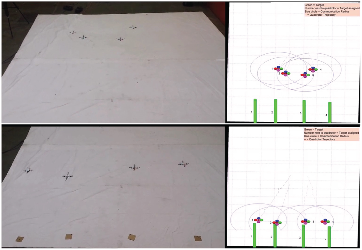
In the first SATO hardware experiment, the quadrotors are placed in a square formation with the targets located 3 m away in a line. The communication radius ( $R_{comm}$ ) for this demo is 1000 mm. The initial locations of the quadrotors are chosen so that every agent can communicate with every other agent creating a connected communication network. The setup for this experiment is shown in Figure 8. This allows the initial auction algorithm to find a conflict-free assignment, which allows the quadrotors to move directly towards their assigned targets. Both the actual trajectories traversed by the quadrotors and the optimal reference trajectories generated by SATO at multiple time steps are shown in Figure 9.

Fig. 8.

Experimental setup for four quadrotors in a connected communication network (see Extension 2).

Fig. 9.

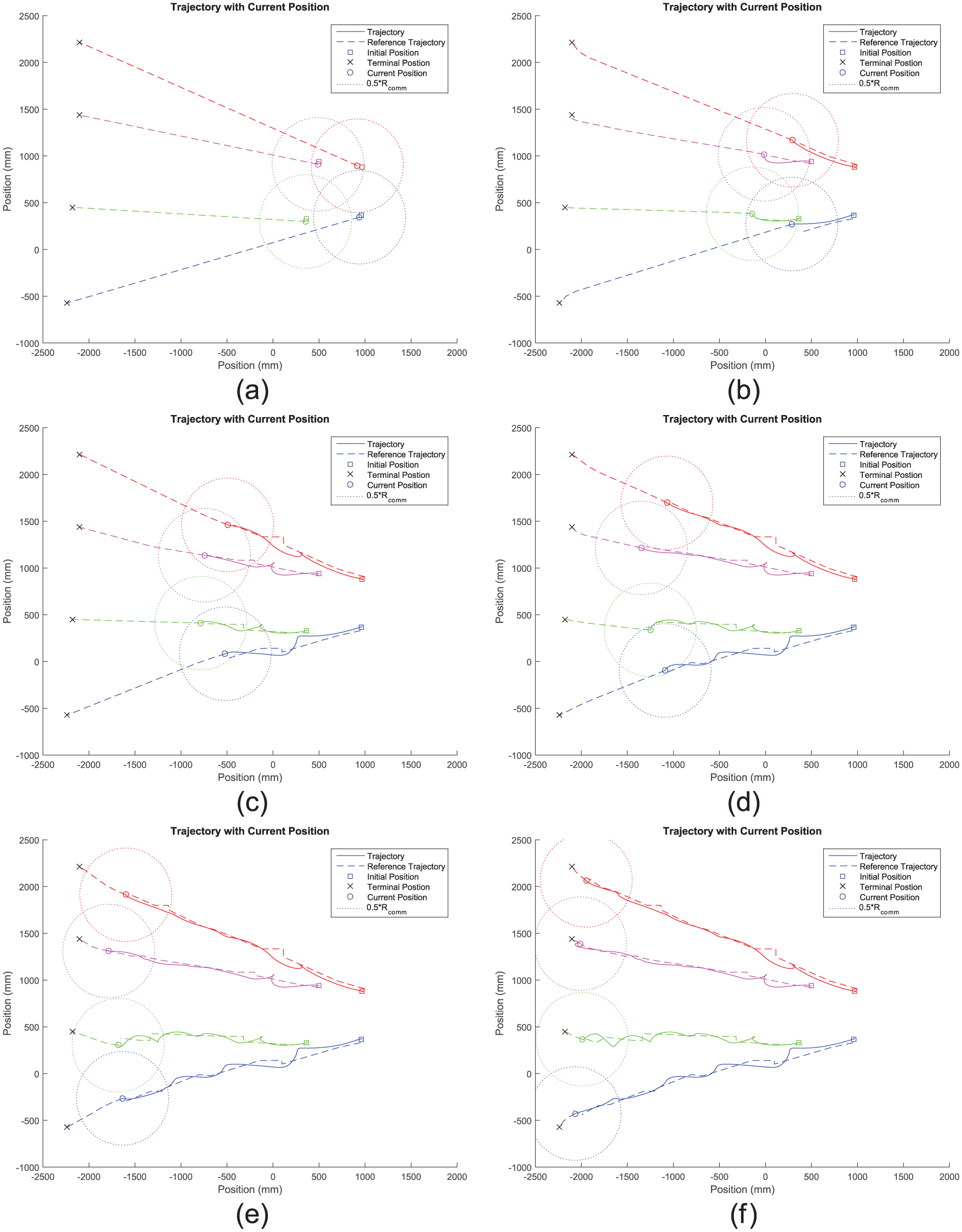
Real-time, optimal trajectories generated by SATO (dashed lines) and actual trajectories (solid lines) throughout a reconfiguration of four quadrotors when the initial communication network is connected. Two quadrotors can communicate when their dotted circles intersect. (a) t = 0 s. (b) t = 3 s. (c) t = 7 s. (d) t = 10 s. (e) t = 13 s. (f) t = 16 s.

The quadrotors are initially located in a square formation with agent 1 (blue) in the bottom right, agent 2 (red) in the top right, agent 3 (green) in the bottom left, and agent 4 (magenta) in the top left. Figure 9 also shows the initial positions of the agents. As mentioned before, the agents can communicate with each other initially, as shown by the intersection of the dotted lines.

Additionally, Figure 9 shows the reference trajectories generated by SATO throughout the reconfiguration. In this figure, the targets (‘x’s) are shown in black to emphasize that any quadrotor can choose any target. Due to the fact that the quadrotors are all on the same communication network at the initial time, the trajectories do not change much throughout the reconfiguration and the agents follow nearly straight lines to their assigned targets.

7.3.2. Real-time flight test with a disconnected communication network

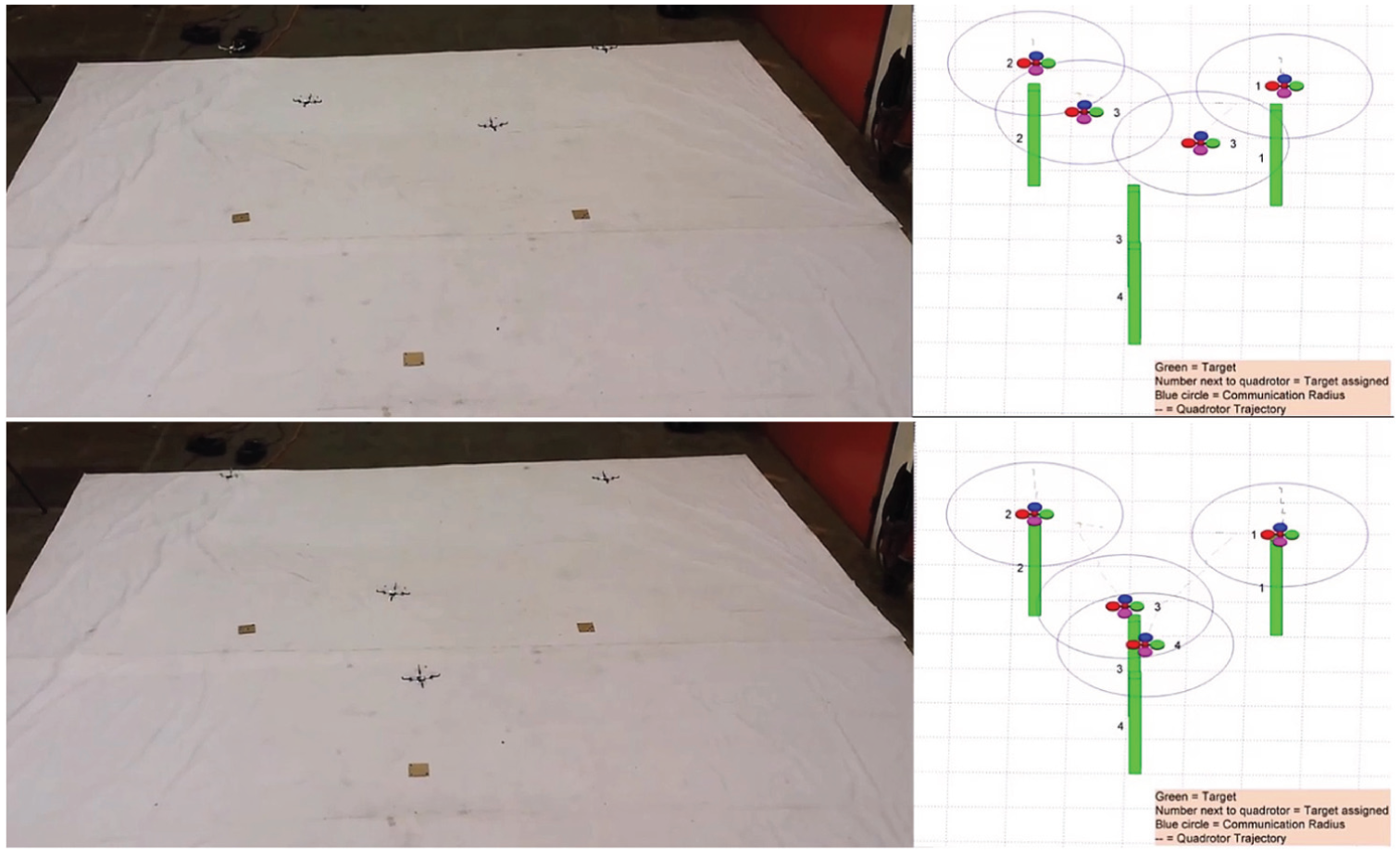
In the second SATO hardware experiment, the communication radius ( $R_{comm}$ ) is 750 mm and the quadrotors are placed in initial positions so that they cannot communicate with each other, which results in multiple agents being initially assigned to the same target. This layout, shown in Figure 10, is intentionally chosen to create several assignment conflicts in order to show how SATO can handle disconnected communication networks. The results of this demonstration are shown in Figure 11.

Fig. 10.

Experimental setup for four quadrotors in a disconnected communication network (see Extension 3).

Fig. 11.

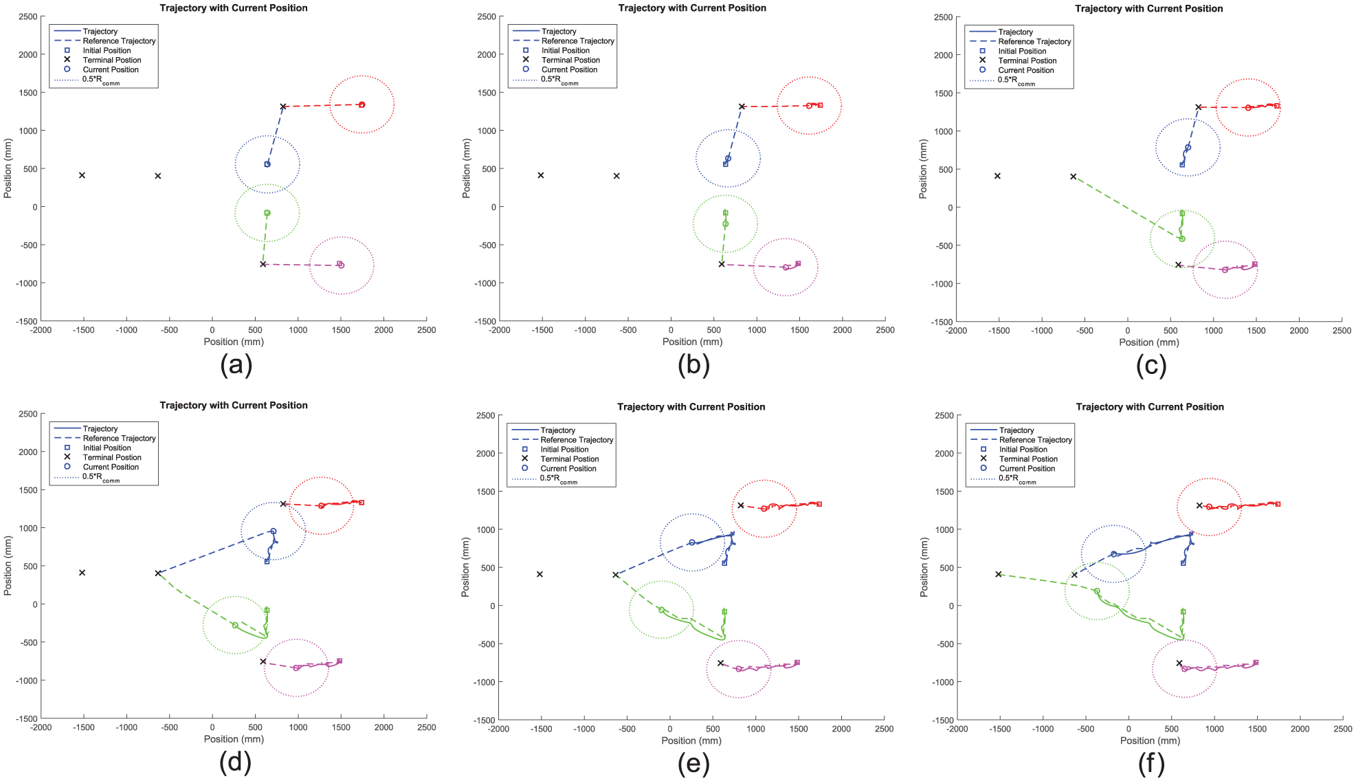
Real-time, optimal reference trajectories generated by SATO (dashed lines) and actual trajectories (solid lines) throughout a reconfiguration of four quadrotors when the initial communication network is disconnected. Two quadrotors can communicate when their dotted circles intersect. (a) t = 0 s. (b) t = 3 s. (c) t = 7 s. (d) t = 10 s. (e) t = 13 s. (f) t = 16 s.

Figure 11 shows the reference trajectories generated by SATO and the actual trajectories traversed by all of the quadrotors throughout the reconfiguration. The quadrotors are initially located in a trapezoid formation with agent 1 (blue) in the top left, agent 2 (red) in the top right, agent 3 (green) in the bottom left, and agent 4 (magenta) in the bottom right. In this figure, the targets (‘x’s) are shown in black to emphasize that any agent can choose any target. In Figure 11(a) and (b), the four reference trajectories terminate at only two targets, which is the result of the two assignment conflicts between agents 1 (blue) and 2 (red) and between agents 3 (green) and 4 (magenta). When the third set of assignments and trajectories are generated as shown in Figure 11(c), agents 3 (green) and 4 (magenta) are able to communicate to resolve the assignment conflict and the third (green) agent’s trajectory terminates at a different target. Similarly, Figure 11(d) shows the trajectories generated by the fourth calculation, which results in agent 1 (blue) being assigned to a new target due to its ability to communicate with agent 2 (red). However, this reassignment creates a new conflict between agents 1 (blue) and 3 (green), which now share the same target. At the fifth computation, shown in Figure 11(e), agents 1 (blue) and 3 (green) still cannot communicate so they remain assigned to the same target. By the time of the sixth computation, shown in Figure 11(f), agents 1 (blue) and 3 (green) can communicate and agent 3 (green) is reassigned to the fourth target.

8. Conclusion

In this paper, we developed a new variable-swarm, distributed auction algorithm to solve the optimal assignment problem for a swarm of agents. The variable-swarm quality allowed the algorithm called VSDAA (Method 1) to adjust the number of targets in the assignment to match the number of agents in the swarm that are bidding on targets. This ultimately resulted in a distributed assignment with the same number of agents and targets. This quality was especially useful when the number of agents in the swarm changed or when there were initially more agents than targets. Additionally, VSDAA (Method 1) can be implemented on a swarm of robots or robotic vehicles with distributed communications and computations while still terminating in a finite number of iterations and achieving the optimal assignment.

We also introduced SATO (Method 3) as an algorithm that integrates the optimal assignment solver, VSDAA, and the trajectory optimizer, SCP. This integrated approach used MPC to update the optimal assignment and trajectory in real time so that changes in the state of each agent and the communication network were included in the new solution. This allowed SATO to ultimately achieve the optimal assignment and trajectory even when the communication network was disconnected at the initial time or when errors prevented the agents from following their optimal trajectories.

Finally, we showed through simulation and experimentation that SATO can be implemented in a variety of situations. Results with double integrator dynamics showed that SATO can overcome an initially disconnected communication network and a loss of a significant number of agents, which cause the communication network to become disconnected. Additionally, a 3-D simulation result using relative orbital dynamics showed that SATO can be run on a swarm of spacecraft even when the dynamics are complicated. The results of these simulations and experiments showed that SATO can be used to solve for the optimal assignment and trajectory in a variety of undesirable conditions in a distributed, real-time manner.

Footnotes

Appendix: Index to Multimedia Extensions

Archives of IJRR multimedia extensions published prior to 2014 can be found at http://www.ijrr.org . After 2014 all videos are available on the IJRR YouTube channel at http://www.youtube.com/user/ijrrmultimedia .

SAGE-Journals-Accessible-Video-Player 10.1177/0278364916632065.M1 0278364916632065_video1 Extension 1

Simulation demonstrating agents forming the shapes U, I, U and C.

The simulation also shows the robustness properties of the algorithm.

SAGE-Journals-Accessible-Video-Player 10.1177/0278364916632065.M2 0278364916632065_video2 Extension 2

Experimental validation of the algorithm using 4 quadrotors.

In this experiment, all the quadrotors initially form a connected graph.

SAGE-Journals-Accessible-Video-Player 10.1177/0278364916632065.M3 0278364916632065_video3 Extension 3

Experimental validation of the algorithm using 4 quadrotors.

In this experiment, all the quadrotors do not form a connected graph in the beginning.

Acknowledgements

Thanks to Saptarshi Bandyopadhyay for stimulating discussions and constructive comments.

Funding

This research was carried out in part at the Jet Propulsion Laboratory, California Institute of Technology, under a contract with the National Aeronautics and Space Administration. © 2016 California Institute of Technology. This work was supported by a NASA Office of the Chief Technologist Space Technology Research Fellowship and an Air Force Office of Scientific Research (AFOSR grant number FA95501210193). Government sponsorship acknowledged.

References

Alfriend

Vadali

Gurfil

. (2009) Spacecraft Formation Flying: Dynamics, Control and Navigation. Oxford: Elsevier.

Alonso-Mora

Breitenmoser

Rufli

. (2012) Image and animation display with multiple robots. International Journal of Robotics Research 31(6): 753–773.

Bandyopadhyay

Chung

Hadaegh

(2016) Nonlinear attitude control of spacecraft with a large captured object. Journal of Guidance, Control, and Dynamics. Epub ahead of print 21 January. DOI: 10.2514/1.G001341.

Bemporad

Morari

(1999) Robust model predictive control: A survey. In: Garulli

Tesi

(eds) Robustness in Identification and Control. London: Springer-Verlag, pp.207–226.

Bertsekas

(1981) A new algorithm for the assignment problem. Mathematical Programming 21: 152–171.

Bertsekas

(1992) Auction algorithms for network flow problems: A tutorial introduction. Computational Optimization and Applications 1: 7–66.

Bertsekas

Castanon

(1991) Parallel synchronous and asynchronous implementations of the auction algorithm. Parallel Computing 17: 707–732.

Boyd

Vandenberghe

(2004) Convex Optimization. Cambridge: Cambridge University Press.

Breger

How

(2007) Gauss’s variational equation-based dynamics and control for formation flying spacecraft. Journal of Guidance, Control, and Dynamics 30(2): 437–448.

10.

Campbell

(2003) Planning algorithm for multiple satellite clusters. Journal of Guidance, Control, and Dynamics 26(5): 770–780.

11.

Campbell

(2005) Collision monitoring within satellite clusters. IEEE Transactions on Control Systems Technology 13(1): 42–55.

12.

Cheah

Hou

Slotine

JJE

(2009) Region-based shape control for a swarm of robots. Automatica 45(10): 2406–2411.

13.

Choi

Brunet

How

(2009) Consensus-based decentralized auctions for robust task allocation. IEEE Transactions on Robotics 25(4): 912–926.

14.

Chung

Bandyopadhyay

Chang

. (2013) Phase synchronization control of complex networks of Lagrangian systems on adaptive digraphs. Automatica 49(5): 1148–1161.

15.

Deters

Ananda

Selig

(2014) Reynolds number effects on the performance of small-scale propellers. In: 32nd AIAA applied aerodynamics conference, Atlanta, GA, 16 June 2014, pp.2014–2151. AIAA Aviation.

16.

Earl

D’Andrea

(2005) Iterative MILP methods for vehicle-control problems. IEEE Transactions on Robotics 21(6): 1158–1167.

17.

Hadaegh

Chung

Manaroha

(2014) On development of 100-gram-class spacecraft for swarm applications. IEEE Systems Journal1–12. Available at: http://ieeexplore.ieee.org/xpl/login.jsp?tp=&arnumber=6880762&url=http%3A%2F%2Fieeexplore.ieee.org%2Fiel7%2F4267003%2F4357939%2F06880762.pdf%3Farnumber%3D6880762

18.

Harary

(1994) Graph Theory. Reading: Addison-Wesley.

19.

Hsieh

Kumar

Chaimowicz

(2008) Decentralized controllers for shape generation with robotic swarms. Robotica 26: 691–701.

20.

Hung

(1983) A polynomial simplex method for the assignment problem. Operations Research 31: 595–600.

21.

Jadbabaie

Lin

Morse

(2003) Coordination of groups of mobile autonomous agents using nearest neighbor rules. IEEE Transactions on Automatic Control 48(6): 2976–2984.

22.

Jongen

Meer

Triesch

(2004) Optimization Theory. Norwell, MA: Kluwer Academic.

23.

Kingston

Egerstedt

(2010) Index-free multiagent systems: An Eulerian approach. In: 2nd IFAC Workshop on Distributed Estimation and Control in Networked Systems, Annecy, France, pp. 215–220.

24.

Kuhn

(1955) The Hungarian method for the assignment problem. Naval Research Logistics 2(1-2): 83–97.

25.

Mayne

Rawlings

Rao

. (2000) Constrained model predictive control: Stability and optimality. Automatica 36: 789–814.

26.

Milutinović

Lima

(2006) Modeling and optimal centralized control of a large-size robotic population. IEEE Transactions on Robotics 22(6): 1280–1285.

27.

Morgan

Chung

Blackmore

. (2012) Swarm-keeping strategies for spacecraft under J₂ and atmospheric drag perturbations. Journal of Guidance, Control, and Dynamics 35(5): 1492–1506.

28.

Morgan

Chung

Hadaegh

(2014) Model predictive control of swarms of spacecraft using sequential convex programming. Journal of Guidance, Control, and Dynamics 37(6): 1725–1740.

29.

Morgan

Chung

Hadaegh

(2015) Swarm assignment and trajectory optimization using variable-swarm, distributed auction assignment and model predictive control. In: AIAA guidance, navigation, and control conference, Kissimmee, FL.

30.

Paranjape

Meier

Shi

. (2015) Motion primitives and 3D path planning for fast flight through a forest. The International Journal of Robotics Research 34(3): 357–377.

31.

Richards

Kuwata

How

(2003) Experimental demonstration of real-time MILP control. In: AIAA guidance, navigation, and control conference, Austin, Texas.

32.

Ross

Fahroo

(2003) Legendre pseudospectral approximations of optimal control problems. Lecture Notes in Control and Information Systems 295: 327–342.

33.

Ruszczynski

(2006) Nonlinear Optimization. Princeton, NJ: Princeton University Press.

34.

Scharf

Hadaegh

Ploen

(2003) A survey of spacecraft formation flying guidance and control (part i): Guidance. In: American Control Conference, Denver, CO, pp. 1733–1739.

35.

Scharf

Hadaegh

Ploen

(2004) A survey of spacecraft formation flying guidance and control (part ii): Control. In: American Control Conference, Boston, MA, pp. 2976–2985.

36.

Schulman

Lee

. (2013) Finding locally optimal, collision-free trajectories with sequential convex optimization. In: Robotics: Science and Systems, Berlin, Germany, June2013. Available at: http://roboticsproceedings.org/rss09/index.html

37.

Subramanian

(2015) Nonlinear control strategies for quadrotors and CubeSats. Master’s Thesis, University of Illinois at Urbana-Champaign, USA.

38.

Turpin

Michael

Kumar

(2014) CAPT: Concurrent assignment and planning of trajectories for multiple robots. The International Journal of Robotics Research 33(1): 98–112.

39.

Vaddi

Alfriend

Vadali

. (2005) Formation establishment and reconfiguration using impulsive control. Journal of Guidance, Control, and Dynamics 28: 262–268.

40.

Chung

Voulgaris

(2015) Target assignment in robotic networks: Distance optimality guarantees and hierarchical strategies. IEEE Transactions on Automatic Control 60(2): 327–341.

41.

Zanon

Campbell

(2006) Optimal planner for spacecraft formations in elliptical orbits. Journal of Guidance, Control, and Dynamics 29(1): 161–171.

42.

Zavlanos

Spesivtsev

Pappas

(2008) A distributed auction algorithm for the assignment problem. In: IEEE conference on decision and control, Cancun, Mexico, pp.1212–1217.

43.

Zhao

Ramakrishnan

Kumar

(2011) Density-based control of multiple robots. In: American control conference, San Francisco, USA, pp.481–486.

Swarm assignment and trajectory optimization using variable-swarm,distributed auction assignment and sequential convex programming

Abstract

1. Introduction

2. Problem statement

2.1 Nonlinear optimal control problem

2.2. Convexification of differential equations

3. Distributed optimal target assignment

3.1. Distributed auction algorithm

3.2. Properties of variable-swarm, distributed auction assignment

4. Optimal trajectory generation

4.1. Decoupling and convexification of collision avoidance constraints

4.2. Sequential convex programming

4.3. Convergence of SCP

5. Swarm assignment and trajectory optimization

5.1. Model predictive control formulation

5.2. Disconnected communication network

6. Simulation results

6.1. Simulation with 2-D double integrator dynamics

6.2. Simulation with 3-D relative orbital dynamics with J 2

7. Hardware experimental results using nonlinear tracking controller

7.1. Robust nonlinear attitude tracking control

7.2. Position tracking controller

7.3. Flight test and experimental results using SATO and position/attitude tracking control

7.3.1. Real-time flight test with a connected communication network

7.3.2. Real-time flight test with a disconnected communication network

8. Conclusion

Footnotes

Appendix: Index to Multimedia Extensions

Acknowledgements

Funding

References

6.2. Simulation with 3-D relative orbital dynamics with $J_{2}$