
Abstract
Teleoperation allows human operators to safely extend themselves to remote environments that are typically difficult or dangerous to access. The remote environments are often unstructured (i.e. not having clear roads or paths to follow) and only accessible by wireless communication (introducing factors such as degraded signals and communication delay). Teleoperated driving under these conditions can result in slow operation speeds and unintended collisions with obstacles. Automating portions of the teleoperation task can help mitigate some of the negative effects of wireless communication. Shared control is used to combine inputs from the human teleoperator and automation. This work presents a new model predictive control based shared control method. We introduce a new representation for obstacle free regions that works well with unstructured robot environments and allows for an model predictive control problem formulation that can be solved rapidly. The shared control method is implemented in a robot simulator and tested with human subjects. Two user studies involving a search task with a mobile robot evaluate the effectiveness of the shared control method and explore its interaction with factors such as communication delay and input interface style. Communication delay is found to have the largest magnitude effect on performance and safety measures. Results demonstrate that the shared control method can improve both performance and safety when delays are present.
Keywords
1. Introduction
As robotic technology continues to develop, humans are able to distance themselves more from dangerous tasks. Control of robotic assets over a distance is referred to as teleoperation and has become a very popular control mode for unmanned ground vehicles (UGVs). Teleoperation of UGVs has been very useful in search and rescue, IED disposal and reconnaissance missions (Chen et al., 2007). One of the challenges with teleoperated UGVs is that their speed of operation is very slow. When manual operators try to drive faster they can end up damaging the UGV by colliding with obstacles or causing it to tip over.
Identifying and steering around obstacles is relatively easy for humans in manned vehicles, however some teleoperation system features inherently make identification and navigation around obstacles difficult. For example, in teleoperation, human operators typically receive information about the robot’s environment through 2D video feeds with low resolution, low frame rate, and limited field of view. To make matters more difficult, this video feed is often delayed hundreds of milliseconds due to video processing and transmission over wireless communication networks.
Many researchers have been working on methods to assist humans in overcoming the challenges inherent to teleoperation. For example, researchers have worked to develop more intuitive interfaces (Nielsen et al., 2007), compensate for delay (Davis et al., 2010), and automate subtasks of the robot mission (Luck et al., 2006). For well defined tasks in structured environments, automation is often a great solution. However, many UGV missions still require some human knowledge or expertise. Cosenzo and Barnes claim most military robotic systems will continue to require active human control or at least supervision with the ability to take-over if necessary (Savage-Knepshield, 2012, Ch. 2). With telepresence robots humans operators want to remain involved (Takayama et al., 2011).
In this paper, we investigate shared control as a means to improve teleoperated mobile robot performance and present a user study that explores the effects of shared control and communication delay. There are two main contributions in this paper. First, we contribute a new technique for representing obstacle free regions that works better in unstructured environments for highly maneuverable mobile robots. The technique is integrated into a shared control method that builds off prior work in robotics, automotive, and aerospace control. Second, based on human subject studies, we develop several relationships that quantitatively describe how factors such as communication delay, shared control, and prediction horizon impact teleoperation performance of a mobile robot.
The remainder of the paper is organized as follows: Section 2 gives a brief overview of the literature in relation to our two contributions. Section 3 describes the obstacle representation technique we have developed and the shared control method we have integrated it into. Section 4 describes the setup for two human subject studies we conducted in relation to our second contribution. Sections 5 and 6 present results and discussion about the relationships we developed. Lastly, Section 7 gives our final conclusions and future work.
2. Background
In the context of our two contributions, we provide a brief review of related work. First, we discuss related human subject studies in robot teleoperation performance and the relationships those studies have found. Second, we discuss shared control methods for obstacle avoidance and techniques for obstacle representations.
2.1. Factors impacting teleoperation performance
Remote operation of robotic assets affords human operators many conveniences and benefits. However, teleoperation performance is impacted by factors such as time delay, degraded feedback of the robot’s environment, and inefficient human-robot interaction schemes. Crandall and Goodrich (2002) suggest breaking down the factors impacting teleoperation performance (referred to as robot effectiveness) into categories of complexity and neglect. Complexity can refer to how difficult the operation task is based on the conditions in the robot’s environment, e.g. density of obstacles, operating speed, time-delay, etc. Neglect refers to how much attention the human teleoperator must give to the system, e.g. how detailed are commands from the human operator, how often must commands be given, etc.
It is well-established that time-delay has a detrimental impact on teleoperation performance, and time delay is known to be one of the most significant factors affecting remote perception and manipulation (Chen et al., 2007). Sources of delay in a teleoperated robot system include network delays, sensing delays, and processing delays (Vozar, 2013). Research efforts in the field of teleoperation have worked to both understand how performance degrades in the presence of communication delay and develop methods of reducing the impact of time delay on performance.
With regards to reducing the impact of delay, some researchers have suggested using a control gain adaptation method that depends on the communication delay in the teleoperation system. For example, Sheik-Nainar et al. investigated performance in a simulated telerover navigation task under conditions of both constant and random delays using different levels of automation. Steering was an input via a joystick, and rover speed was automatically adjusted based on delay to maintain stability. The study found that gain adaptation (primarily an adjustment of speed based on the delay in the system) was able to improve navigation performance for direct teleoperation (Sheik-Nainar et al., 2005).
Researchers have used augmented reality to display additional information to human operators and improve teleoperation performance. For example, augmented reality has been used to assist the human operator in estimating the robot’s actual location. Studies have shown that predictive displays have been helpful for driving tasks with both short delays (approximately 400–1100 ms) (Davis et al., 2010) and multi-second delays (Matheson et al., 2013). Augmented reality has also been used to render 3D video projections and create simulated exocentric views of the robot’s environment that improve teleoperation performance (Ferland et al., 2009; Kelly et al., 2011).
Another method to improve teleoperation performance has been through the use of different control interfaces. The idea of a steerable waypoint has been used in control of military robots (Metcalfe et al., 2010) and telepresence robots (Takayama et al., 2011). The idea behind the steerable waypoint is that the user can continuously update the location of a waypoint out ahead of the robot. The robot will have a controller that tries to track towards wherever the location of the waypoint is. Safety features, such as obstacle avoidance, can be included in the controller that plans the path towards the waypoint location. Experimental results with the steerable waypoint method have often shown that while the number of errors might be reduced, task completion time often increases with the steerable waypoint (Metcalfe et al., 2010; Takayama et al., 2011).
Advancements in sensing/perception and available computational power have also resulted in an increasing number of autonomous features on-board teleoperated robots. Prior work describes the notion of adjustable autonomy (Goodrich et al., 2001), where the robot may be able to have operating modes ranging from a pure teleoperation mode to fully autonomous mode. In between these two extremes are a spectrum of semi-autonomous control modes (see Fig. 1). Determining how and when to switch between different semi-autonomous modes to give the best overall teleoperation system performance is still challenging (Chiou et al., 2015). Additional discussion of semi-autonomous control methods is included in Section 2.2.
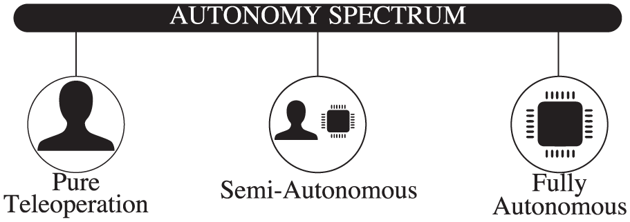
Diagram showing autonomy spectrum.
Many studies have looked at how communication delay impacts pure teleoperation performance going back to Sheridan and Ferrell (1963). Additionally, many researchers have developed and compared performance with semi-autonomous control methods to pure teleoperation (Macharet and Florencio, 2012). However, there are few studies that have investigated the interaction between communication delay and semi-autonomous control. One such study that has investigated this interaction was by Luck et al. (2006). Luck et al. found that for a mobile robot driving task with no time delay, course completion time was hardly impacted by the level of autonomy on the robot. This motivates the questions: under what delay conditions does semi-autonomous control improve performance? With which semi-autonomous control methods/interfaces does time delay degrade performance most?
2.2. Shared control methods
Semi-autonomy (Fig. 1) includes many levels of control division between the human operator and the autonomy, often referred to as levels of automation (LOAs). There are several different standards for describing the level of automation. For example, there is the SAE levels of driving automation (On-Road Automated Driving (ORAD) Committee, 2014) the NHTSA levels of vehicle automation (Administration et al., 2013), Autonomous Levels for Unmanned Systems (Huang, 2007), Levels of Automation (Endsley, 1999), and Levels of Robot Automation (Beer et al., 2014) to name a few. The control method we develop can best be described as shared control in the context of Endsley and Kaber’s levels of automation (Endsley, 1999). We will compare the results with the shared control automation level to pure teleoperation and full autonomy, so that the full spectrum is covered.
There has been significant prior work in developing shared control methods. Design of shared control methods is a two part process: (1) an autonomous planning/control method must be selected/designed, and (2) a control arbitration must be selected/designed. The control arbitration determines how control is divided between the human operator and autonomy. Control arbitration is often described by the very simple function
In the area of motion planning and obstacle avoidance, prior work has investigated using artificial potential fields (Khatib, 1986), the vector field histogram (Borenstein and Koren, 1991), dynamic window (Fox et al., 1997), and model predictive control (MPC) (Anderson et al., 2010). Artificial potential fields require little computational power, but typically do not consider vehicle kinematic and dynamic constraints. The vector field histogram and dynamic window methods are able to consider some vehicle dynamics, but are limited in the complexity of the model they can consider. MPC based obstacle avoidance methods have become most popular recently due to improvements in computing power and optimization solvers. While MPC based methods tend to be computationally more expensive than previous methods, they are able to use accurate models of the vehicle and its environment to calculate optimal paths. MPC based methods can scale well from simple vehicle models to complex nonlinear models depending on the computing resources available. The control designer has much flexibility over how to define the cost function and what to define as optimal. Integrating a human operator into the MPC loop is currently an area of active research (Anderson et al., 2014; Chipalkatty et al., 2013; Erlien et al., 2014; Shia et al., 2014).
Two of the main challenges with human-in-the-loop MPC are (1) estimating human input over the MPC solution horizon, and (2) formulating the MPC problem such that it can be solved fast enough. With regards to estimating the human input over the MPC horizon, some researchers simplify this challenge by assuming the human input or a position the human is trying to move towards is known (Anderson et al., 2014; Erlien et al., 2014). This assumption is reasonable in many situations, e.g. driving in structured highway environments, or when solving the MPC problem for short solution horizons. If the exact goal of the human operator is not known, but a few candidate goals are known, then Javdani et al. (2015) have suggested a method of probabilistically estimating the goal based on a history of inputs. Other researchers have suggested methods of generating a probabilistic estimate of the human input or desired trajectory using past human operator data (Dragan and Srinivasa, 2013; Hauser, 2013; Shia et al., 2014).
With unlimited computation power, one might imagine formulating the MPC problem to contain a very detailed dynamic model of the robot being controlled and its environment. However, high fidelity dynamic models of robots are often nonlinear and representations of safe regions for robot navigation in an environment with obstacles are often non-convex. More recent advances in optimization methods have made including nonlinear dynamics (as long as the problem is still convex) possible without large sacrifices in computation time (Andersen et al., 2015). However, non-convex optimization is still challenging to do quickly and it is difficult to guarantee convergence to a globally optimal solution. As a result, some prior work has used optimization methods that focus on finding the best of a group of local minima (Hauser, 2013). Other researchers have focused on how to formulate the MPC problem as a convex optimization problem. Non-convex constraints often arise when mathematically representing the feasible regions for the robot to move in the environment. In general, researchers have tried to define a single or multiple convex region that approximates the non-convex space.
Liu et al. have suggested partitioning the non-convex feasible region of the robot using triangular sections constructed from each visible obstacle corner (Liu et al., 2014). With this set of convex feasible regions, they formulate a multi-stage optimal control problem to handle the transitions between each of the feasible regions and calculate the optimal control input (Liu et al., 2014). Similarly, Diets and Tedrake have developed a method (called IRIS) of segmenting a non-convex obstacle free space into several convex regions that approximate the non-convex space (Deits and Tedrake, 2015a). Diets and Tedrake have demonstrated that with IRIS they can formulate the path planning and obstacle avoidance problem for a UAV as a mixed-integer programming problem (Deits and Tedrake, 2015b). Both Liu and Diets have demonstrated that their optimization formulations can be solved on time-scales on the order of seconds using only laptop computing resources (Deits and Tedrake, 2015b; Liu et al., 2015). Solve-times on this time scale work well for trajectories that can be pre-planned, but for uninterrupted operation with a human-in-the-loop, faster solve times are required.
Erlien et al. use an environmental envelope representation for the feasible region of the vehicle in a highway operation scenario with an obstacle in the road. The environmental envelope applies a constraint on the vehicle’s lateral position in the MPC formulation by assuming the vehicle will continue moving forward at a constant speed along the road (Erlien et al., 2014). Similarly, Anderson et al. construct a homotopy of the safe regions that the vehicle can feasibly travel. The homotopy representation is then converted into constraints on the vehicle’s lateral position in the MPC problem, based on assumptions of the vehicle’s path forward. Both convex approximations by Erlien et al. and Anderson et al. allow for rapid solving of the MPC problem (multiple times per second) and are well suited for highway type scenarios (Anderson et al., 2014). However, these methods are not well suited for operation in less structured driving scenarios, e.g. a mobile robot that is not following a road and could be rapidly turning around to head in the opposite direction.
The aerospace industry has similar challenges in path planning and obstacle avoidance that occur in environments without obvious roads or paths to follow. This problem has been approached by using hyperplanes to segment off areas free of obstacles. However, selecting static hyperplane constraints can result in a very conservative representation of the safe region for the vehicle. By allowing the hyperplane constraints to vary over the MPC solution horizon, a less conservative representation of the vehicle’s feasible region can be created while still allowing the MPC problem to be solved rapidly in real-time. One such method of varying the hyperplane constraints is by allowing the constraints to rotate around the edges of the obstacles they bound (Petersen et al., 2014). More details about using rotating hyperplanes to construct convex feasible regions will be discussed in Section 3.2.
3. Shared control method
In this paper, we consider a generic search task (abstracted from a mission that might be encountered in reconnaissance or search and rescue) for a small mobile robot. In this task, the automation available on the robot is assumed to have some computational resources and capabilities to sense obstacles, however it does not have the ability to complete the search task alone (e.g. it cannot detect certain objects of interest). The question we will explore is how to effectively share control between the human and automation in this scenario.
We chose to use model predictive control (MPC) in our shared control method for reasons outlined in Section 2.2. The MPC will handle both obstacle avoidance and control arbitration. Instead of explicitly calculating an
3.1. Model predictive control formulation
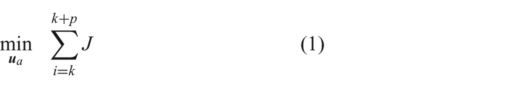
The shared control method is formulated using MPC in the following way


where
Variable
Note that in the formulation of equations (1) to (4), all constraints are linear. Additionally, we select the cost function J to be quadratic. Thus, our shared control method is represented as a convex quadratic programming problem and can be efficiently solved. We use the CVXGEN tool to generate a solver that can easily find a solution to our problem in real-time (Mattingley and Boyd, 2012).
3.2. Obstacle constraint representation
When obstacles are placed in a robot’s environment, they create a “hole” in the obstacle-free space. The representation of this obstacle-free space becomes non-convex. Solving optimization problems with non-convex constraints is challenging to do rapidly and many researchers have proposed convex approximations for obstacle-free regions as described in Section 2.2. This section will describe the convex approximation method we developed for the MPC problem and why we believe it is well suited for highly maneuverable robots in unstructured environments.
3.2.1. Convex approximations
To describe a convex region free of obstacles, one could cleverly place a set of hyperplane inequalities to exclude all obstacles. In most cases, the resulting region would miss much of the obstacle free region. To overcome this shortcoming, prior work has suggested defining multiple convex regions to approximate a non-convex space. Recall that the MPC problem consists of solving equations (1) to (4) over the prediction horizon. A challenge that arises with considering multiple convex regions is determining which convex region to consider at each step of the prediction horizon. Two approaches have been used to address this challenge. The first is to make the selection of the convex region part of the solution by formulating a multi-stage optimal control problem (Liu et al., 2014) or a mixed-integer programming problem (Deits and Tedrake, 2015b). The second is to estimate which convex region should be used at each step of the prediction horizon and specify that estimate to the MPC problem (Anderson et al., 2010; Erlien et al., 2014).
The first approach creates an optimal control problem that is much easier to solve than the original problem with non-convex constraints. The optimal control problem can be solved on the order of seconds and it works well for robots with full autonomy or supervisory control that can pre-plan large portions of movement without human operator input (Deits and Tedrake, 2015b). However, for shared control with the human operator providing regular inputs, the MPC problem must be solved more rapidly - several times per second. By estimating which convex region should be used at each step of the prediction horizon, the resulting MPC problem can be solved multiple times per second.
The methods developed by Anderson et al. (2014) and Erlien et al. (2014) consider Ackermann steer vehicles moving at higher speeds. They construct corridors (referred to as an environmental envelope in Erlien et al. (2014) and a homotopy in Anderson et al. (2014)) consisting of multiple convex regions to describe the area that the vehicle will travel through to reach its end goal. Based on the corridors and an assumed forward velocity for the vehicle over the prediction horizon, they apply constraints on the lateral position of the vehicle to avoid colliding with obstacles. This method has been shown to work well with full size Ackermann steer vehicles.
However, the corridor method is not well suited for skid-steer robots operating at lower speeds in environments without paths or roads. Under these operating conditions, the robot may not drive down a corridor straight ahead in between obstacles. Instead it may turn sharply to the right or completely around to head in the opposite direction and the lateral constraints from the corridor method could be meaningless for obstacles in the new direction in which the robot is heading.
For these conditions, with a highly maneuverable robot in an unstructured environment, we propose a new method for representing convex, obstacle free regions. Using a set of hyperplane inequalities, we define a convex, obstacle free region that contains the robot’s initial position. Over the course of the MPC prediction horizon, this convex, obstacle free region changes in shape to include more area in the direction that the robot is predicted to move, while still making sure the robot’s initial position is contained in the final region.
For simplicity, we will describe the method used to construct the convex, obstacle free regions for the 2D case, but the method could be extended to the 3D case (e.g. for quadcopters or underwater robots). In the 2D case, the hyperplane inequalities are simply straight line, linear inequalities. We consider one linear inequality for each of the n closest obstacles. In our implementation, we considered
3.2.2. Algorithm description
Our method is described in Algorithm 1 with descriptions for each of the subroutines in the text that follows. Refer to Fig. 2 for additional description. In general, Algorithm 1 can be applied to environments with obstacles that are convex or can be bounded by ellipsoids.
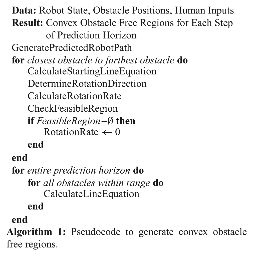
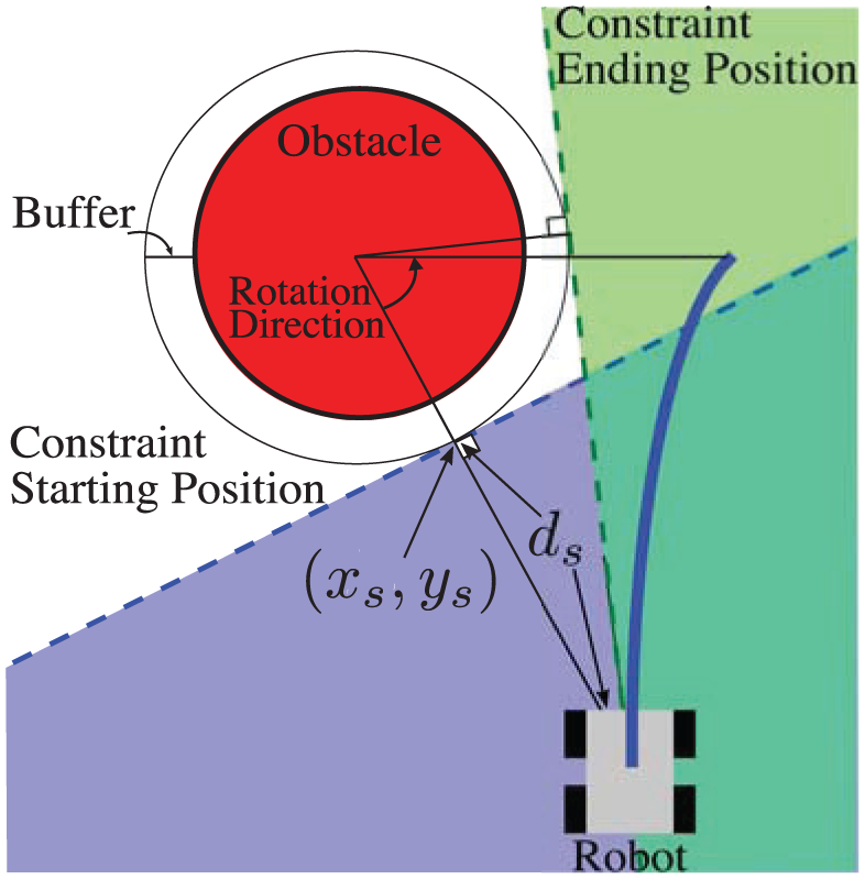
Diagram describing obstacle representation as linear constraints in MPC problem formulation.
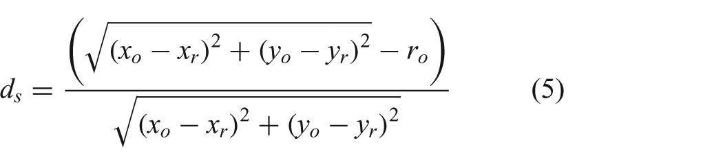


where

The inequality sign is then selected such that any point inside the obstacle does not satisfy the inequality.
The rotation rate for each obstacles linear inequality will depend on the end position of the constraint and the length of the prediction horizon. The end position of the constraint is defined to be tangent to the ellipse bounding the obstacle and pass through the center of the robot. Note that two lines will satisfy these criteria. The rotation direction determines which line to use,i.e. the line that is encountered first when rotating the starting constraint in the rotation direction and keeping it tangent to the ellipse.

where
3.2.3. Algorithm discussion
A visual representation of generating the obstacle free convex regions is shown in Fig. 3. The red circles represent obstacles. The left sub-figure considers a projected robot path (solid blue line) for a left turn and the right sub-figure considers a right turn. In each sub-figure, the obstacle free region at the start of the prediction horizon is represented by the lightly shaded blue region enclosed by the dashed blue lines. As the prediction horizon goes on, the linear inequalities tangent to the obstacle will rotate around until it reaches the dashed green line at the final step of the prediction horizon. The obstacle free region at the end of the prediction horizon is represented by the lightly shaded green region enclosed by the dashed green lines. One can see that as the robot’s predicted position moves towards the obstacles, the constraints will adjust to allow for a wider range of motion while still keeping the robot’s initial position in the feasible region.
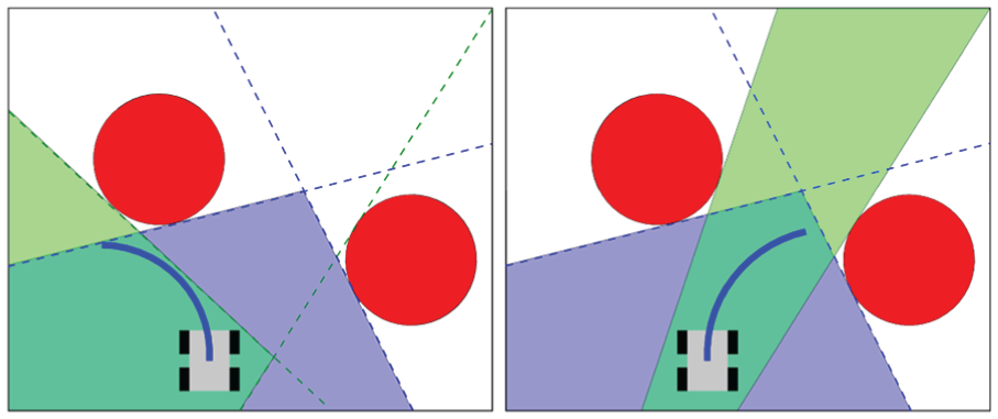
Obstacle constraints with multiple obstacles for two different predicted robot paths. The initial feasible region is represented by the light blue shaded area. The dashed blue lines rotate about the center of the obstacles they are tangent to over the prediction horizon until they reach the positions of the dashed green lines. The feasible region at the end of the horizon is represented by the light green shaded area.
One note on implementation issues: the robot may end up near the edge of the feasible region and small errors may push the robot into the infeasible region. To accommodate this issue, the ellipse enclosing the obstacle can include an added buffer zone, so that it is slightly larger than the obstacle it is enclosing (see Fig. 2). In our implementation, we used a buffer of 0.15 m. When the robot is near the edge of the feasible region, the overall radius of the obstacle is reduced by 0.05 m to move the robot out of the infeasible region.
Similar to most other convex approximation methods, our algorithm is a conservative estimate of the true non-convex space. The algorithm assumes the robot is not initially inside an obstacle and can be applied when obstacles can be bounded with a strictly convex curve, such as a circle or ellipse, that does not intersect with other curves bounding obstacles. The method could be extended to consider curves that are not strictly convex (i.e. curves that contain straight line segments) and curves that intersect. To consider curves containing line segments, one would need to develop a rule for determining the slope of the linear inequality at points where two line segments meet (i.e. where the slope may be undefined). If two or more convex curves bounding obstacles intersect, then one would likely want to impose a rule that the linear inequalities should not rotate along the curve past the intersection point.
Based on the algorithm we defined and conditions described above, we can guarantee the constraints generated will be linear and convex. This guarantee holds because the linear inequality calculated for each obstacle can be more generally described as a half-space, which is a convex set. The intersection of an arbitrary collection of convex sets is convex (Rockafellar, 2015, Ch. 2).
Our algorithm can generate constraints very rapidly, making it well suited for optimization problems that need to be solved on the order of milliseconds. It is best suited for shorter prediction horizons. As the prediction horizon increases, the algorithm may feel more limiting because the robot’s initial position is kept in the feasible region. The algorithm can apply constraints to robot positions in 2D and 3D space, rather than the 1D constraints on lateral position with the environmental envelope method (Erlien et al., 2014) that are often used with Ackermann steer vehicles moving forward at constant speeds. Thus, our obstacle constraint representation is better suited for skid-steer and omni-directional robots.
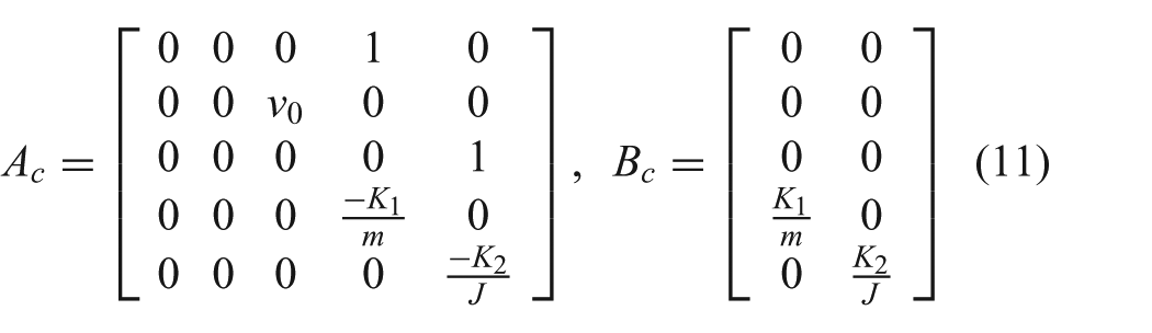
3.3. Robot model
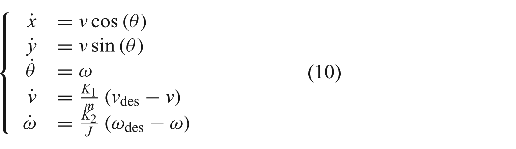
The simple skid-steer robot shown in Fig. 4 is considered. A linearized model based on a dynamic unicycle robot model (Carona et al., 2008) is used in the MPC formulation. This type of model is commonly used to describe the behavior of skid-steer and differential drive robots
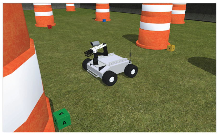
Exocentric view of simulated UGV that was teleoperated in the human subject studies.
In the equations above x, y represent the robot’s planar position,
In order to make equation (10) more efficient for use in the MPC formulation, the equations are first linearized by applying the small angle approximation. This changes the first two equations of equation (10) to
Values for
3.4. Cost function
Many different cost functions could be selected for this shared control method. To enable solving in real-time, we selected a quadratic cost function
Notice that the cost function selected only depends on the shared control input
A subscript i has been included on the weighting matrix
The cost function we selected is similar to that proposed by Chipalkatty et al. (2013). The main differences are the ability to weight the cost on forward speed and turn rate in different proportions and the feature of decreasing weights over the prediction horizon.
With the cost function selected in equation (12), the solution to equations (1) to (4) will match the estimated human input as closely as possible without violating constraints on the robot dynamics or colliding with obstacles. If the estimated human input is not predicted to cause any collisions, then the solution
Alternatively, the cost function can be easily modified to instead follow a desired path defined by a set of robot states
This variation of the cost function depends on the shared control method state
The modified cost function in equation (13) can be used for shared control modes that are able to estimate a desired path to follow or a desired waypoint.
3.5. Human model
The shared control method presented in this paper does not assume knowledge of an end goal position for the robot. Instead, the MPC method tries to match an estimated human input or goal position. Recent work has proposed a method of predicting user intention for manipulator arm control via learning from training data (Dragan and Srinivasa, 2013). Similarly, Shia et al. (2014) have a method of creating a probabilistic driver model that can be fitted to training data. Bohren et al. (2016) do not require training data to predict manipulator arm movement in teleoperation. Instead they propose a method of predicting movement intent from a graph of possible actions.
While these methods have been shown to offer improvements in performance, prior work has also shown that even simple prediction methods (such as a zero-order hold) of the human’s input can be effective for short horizons. For example, Chipalkatty et al. (2013) have shown that using a zero-order hold to estimate the human operator inputs performs as well as a least squares system identification method. Since the MPC problem formulation in our human subject study is solved at a rapid rate and the prediction horizon is relatively short (0.5–1.5 s), we will consider a zero-order hold of the human operator’s current input. That is, each time the MPC problem is solved, the values of
We believe that this simple, zero-order hold prediction method is a reasonable design decision for the user study given rapid update rate and relatively short prediction horizon of the MPC problem. A word of caution - in teleoperation systems with communication delays over one second, prior work has said that human operators often change to their control strategy to a move-and-wait operation mode (Chen et al., 2007). The move-and-wait operation mode may require a different type of human model than the zero-order hold method. However, our user study considers delays less than a second. Future work could include more advanced methods mentioned above for estimating the human input over the prediction horizon.
4. User study description
The shared control method we developed was used in two sets of human subject studies. The studies investigated the effectiveness of the shared control method, as well as the impact of several critical factors in teleoperation discussed in Section 2.1.
Subjects drove a mobile robot around an environment filled with obstacles to search for objects of interest (OOIs) scattered throughout the space, similar to search and exploration missions. Subjects were told that the robot could sense obstacles and help avoid them in shared control mode, but the robot was not capable of sensing the OOIs. Due to the time limits we imposed, it was not possible for the robot to explore the entire area. Subjects had to prioritize which areas they searched.
As a motivating example, a robot could be enlisted to search for survivors in a disaster area, but not have the proper sensor that can distinguish humans from animals or other objects. There may not be time to add the sensors that could make such a distinction in recognizing survivors. Additionally, if time is critical, it may not be ideal for the robot to exhaustively search the whole area. A person experienced in disaster response may have expertise in prioritizing search areas that are more likely to have survivors. That person would want to have more control over where the robot navigates and their decision on where to explore next could be triggered by subtle observations.
4.1. Robot environment
In both human subject studies, participants performed a timed search task. Subjects operated a virtual skid-steer robot in an environment simulated with ANVEL (Durst et al., 2012). ANVEL is free robot and vehicle simulation tool developed by Quantum Signal, LLC. It is built on popular open source libraries including the open dynamics engine (ODE) for simulating nonlinear dynamics/physics and the object-oriented graphics rendering engine (OGRE) for generating high fidelity, realistic graphics.
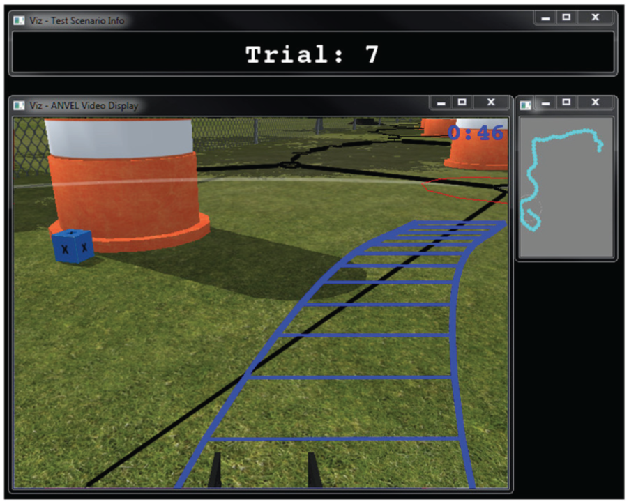
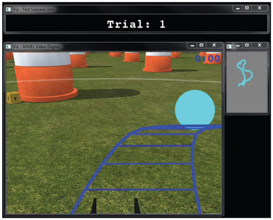
Each environment consisted of a rectangle enclosed by concrete barriers or chain-link fence. The dimensions of the environment, number of obstacles, and number of OOIs was the same across trials in each user study. However, the placement of the obstacles and OOIs were randomized in each trial. The OOIs were represented in the environment using small colored boxes with a letter printed on each side of the box face. A sample OOI can be seen next to the barrel in Fig. 5.
Visual display shown to participants for Interfaces A, B, and C in the human subject studies.
The robot was assumed to have sensors (e.g. LIDAR, stereo camera, sonar) that could sense obstacles locally. Only obstacles within the robot’s sensing field of view (
4.2. User interface
A total of five different user interfaces were used. Details on which user interfaces were used in each study will be made clear in the test condition description (Section 4.4).
Interface A - human operator manually controls robot velocity commands.
Interface B - shared control with autonomy trying to match human operator velocity commands. Autonomy is located on-board the robot.
Interface C - shared control with autonomy trying to match human operator velocity commands. Autonomy is located at the operator control unit.
Interface D - shared control with autonomy following Voronoi map paths based on human operator commands. Autonomy is located on-board the robot.
Interface E - shared control with autonomy tracking towards a waypoint. Human operator actively controls the waypoint location. Autonomy is located on-board the robot.
As many features as possible were attempted to be kept the same across interfaces. The basic visual display shown to users in the human subject study is shown in Fig. 5. The largest display shown in Fig. 5 is a simulated video feed from a camera attached to the robot’s manipulator arm. The video was displayed at 25 fps with a resolution of 640x480 pixels. The video has a few annotations to better help users complete each trial. The top right corner of the video display shows users a clock that counts down the time remaining in their current trial. The translucent white arc extending from the left to right side of the video screen indicates the robot’s maximum sensing distance of 4 m. Obstacles within this arc can be detected/avoided and OOIs can be identified.
The last annotation feature on the video display is the two blue lines. These lines represent the projected path of the left and right side wheels of the robot over the prediction horizon. For Interface A, the blue lines show the robot’s predicted path using the zero-order-hold human model and ignoring potential collisions with obstacles. For Interfaces B-E, the blue lines show the robot’s predicted path from the model predictive control (MPC) problem solution.
Since much of the environment looks similar, an overhead miniature map is provided on the top right side of the video display. As subjects drive the robot around, teal dots are displayed on the map every two seconds to indicate areas the robot has been. This was done to help subjects travel to areas they had not explored yet, but was not intended to provide enough information to navigate without the video display.
Test subjects controlled the simulated robot using a wireless XBox controller. For Interfaces A-D, driving controls were similar to those of racing games, where the right trigger was used to control forward speed and the left joystick controlled turn rate. For Interface E, the right trigger also controlled robot forward speed, however the left joystick adjusted the position of the steerable waypoint on the screen. Subjects could turn in place using the right joystick in all Interfaces.
In addition to using the XBox controller for driving, subjects used the X-Y-A-B buttons to identify OOIs. The color-letter combinations of the OOIs were the same as the those on the XBox controller. In order for an OOI to be identified, it had to be within the sensing range and the subject had to double tap the corresponding button. Once identified, a ding sounded and the OOI turned translucent.
The following is a more detailed description of the differences among interfaces.
4.2.1. Interface A
Human operators had no assistance from the autonomy. Robot velocity commands from the gamepad were passed to the robot, regardless of whether they would cause a collision.
4.2.2. Interface B
The MPC problem is solved on-board the actual robot (see Extension 1). As a result, the commands that the MPC problem receives from the human operator will be delayed and the projected path from the MPC problem displayed on the human operator’s camera view will be delayed. However, the information about robot state and obstacle location used in the MPC problem will be undelayed. Interface B uses the cost function in equation (12).
4.2.3. Interface C
The MPC problem is solved at the operator control unit. As a result, the commands from the human operator and information displayed on the camera view will be undelayed. However, information about robot state and obstacle location used in the MPC problem will be delayed. Model-based predictors are used to obtain estimates of the robot and its environment’s undelayed state information. Interface C uses the cost function in equation (12).
Since the control commands will experience delay before reaching the robot, the commands calculated for the entire prediction horizon are sent from the operator side to the robot with a timestamp. Then, based on the difference between the current time and the timestamp of the delayed command, the robot selects the command intended for the current time. For example, if a packet of control commands is 300 ms old, then the robot will begin applying control commands starting 300 ms into the prediction horizon.
Given the success of predictive based control methods (e.g. MPC) and model based predictors, we hypothesized that these predictive methods could compensate for the delay better than the human operator could. The robot’s projected path will be more responsive to user inputs, but errors in the estimates of the robot and environment state will likely result in more collisions. The second user study discussed in this paper will explore Interface C in comparison to Interface B.
4.2.4. Interface D
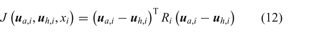
The MPC problem is solved on-board the robot. From the human operator model, a projected robot path is generated. The MPC problem will then be solved to have the robot move towards the point on the Voronoi map closest to the end-point of the robot’s projected path. The Voronoi map is displayed using black-lines on the ground in the human operator’s camera view (see Fig. 6). The point on the Voronoi map that the MPC problem is currently trying to move the robot towards is shown to the human using a red circle. Interface D uses the cost function in equation (13).
Visual display shown to participants for Interface D in the human subject study.
The Voronoi map was generated beforehand for each environment. However, it would be feasible to generate the Voronoi map locally in real-time based on local environment information.
4.2.5. Interface E
The MPC problem is solved on-board the robot. The human operator controls the
Visual display shown to participants for Interface E in the human subject study.
4.3. Test procedure
Each study began with subjects filling out an informed consent form and answering basic background questions. Following this, subjects underwent a training session to make sure they had achieved a level of robot operation competency that would allow them to perform the search task. The training portion took approximately 10–15 minutes and consisted of the following parts.
Subjects were verbally instructed how to drive forwards, backwards and turn in an empty environment.
The robot’s projected path represented by the blue lines was explained to subjects as they continued to practice driving in the empty environment.
Subjects practiced identifying a series of OOIs that were placed in a straight line ahead of them.
For each interface tested, subjects were placed in an environment with four obstacles and told to practice driving around them.
Subjects had the opportunity to complete a practice trial with each interface that was setup identically to the scored trials. In the practice trials, subjects experienced communication delay both in their commands sent to the robot and in the video sent back to them.
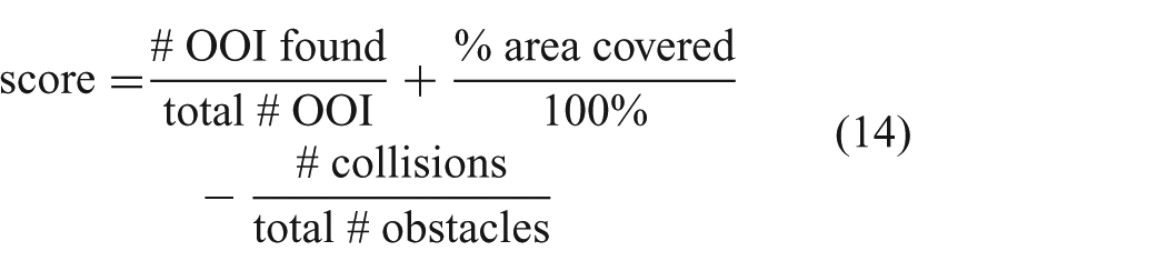
After the training and practice trials were completed, subjects moved on to the scored trials. Each scored trial was two minutes long. Participants were instructed to explore as great an area as they could, identify as many OOIs as possible, and avoid collisions with obstacles. To incentivize participants to try their best in each of these three tasks, a bonus compensation was offered to participants with the highest scores. A combined score metric was explained to subjects and they were told that the top score for each trial would be paid bonus compensation of $10 in addition to the $10 they received just for participating. The combined score metric was calculated as follows
Following each scored trial, subjects filled out a subjective survey to gauge their sense of presence and delay in the robot environment. After the scored trials and surveys, subjects were thanked for their participation and dismissed. Each user test took approximately one hour.
4.4. Test conditions
Twenty different subjects were recruited for each of the studies. There were a total of twelve scored trials in the first study and eight scored trials in the second study. The first human subject study used a three-way repeated measures study design to evaluate human subject performance under communication latency, shared control, and different prediction horizons. The second study used a two-way repeated measures design to evaluate factors of communication latency and interface (see Table 1). The order of the trials was randomized among subjects.
Test conditions for each human subject study.
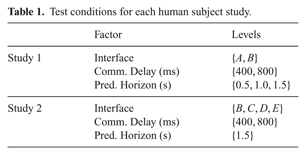
The communication delay was introduced in two places - from human to robot (H2R) and from robot to human (R2H), as shown in Fig. 8. The delay from R2H was selected to be larger than from H2R because we assumed additional delay would be introduced as a result of video processing and higher bandwidth requirements to send information from robot to human. Although wireless network communication delays are often time-varying, constant (time-invariant) communication delays were tested in the human subject studies. Constant delays were selected: 1) to reduce the number of factors in our user study design, and 2) because our prior work suggests that teleoperation performance with time-varying delays can be related to performance at constant delays (Storms and Tilbury, 2015). The two communication delays tested were 400 ms (100 ms H2R, 300 ms R2H) and 800 ms (300 ms H2R, 500 ms R2H). These values are in line with those reported in studies on communication latency in video chat (Xu et al., 2012).
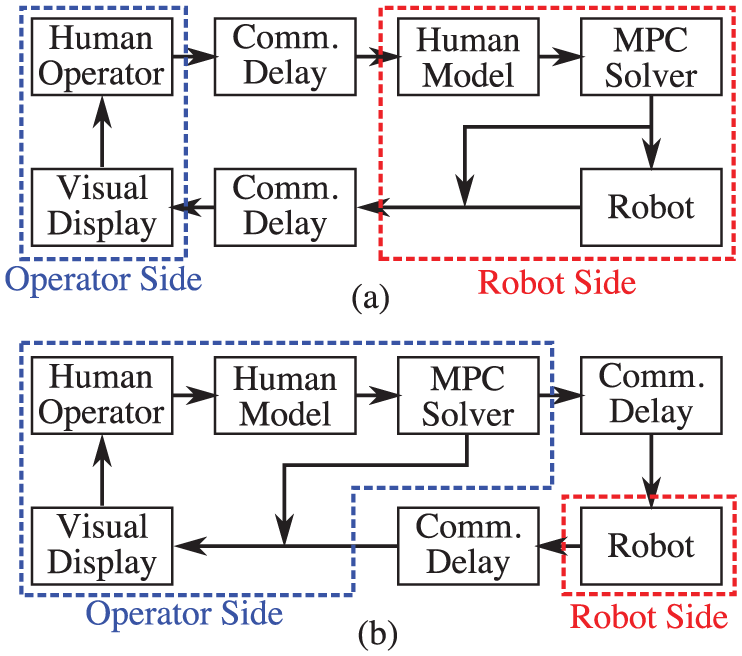
Functional diagram of information exchanged among components of the teleoperation system. Diagram (a) describes the arrangement for Interfaces A, B, D, E and (b) describes the arrangement for Interface C.
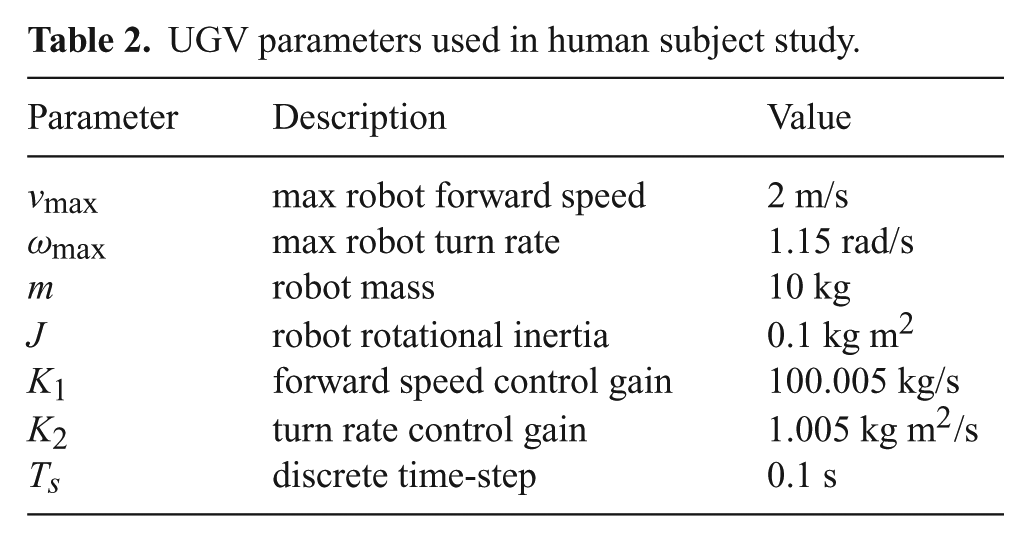
In user study 1, each arena had dimensions 24×36 m and a total of 15 OOIs. We noticed that a couple of the top performers in user study 1 identified all 15 OOIs. Thus, for user study 2, the arenas were increased to have dimensions of 30×42 m and a total of 20 OOIs to prevent subjects from saturating the number of OOIs identified. A summary of the robot parameters used for the MPC are given in Table 2.
UGV parameters used in human subject study.
4.5. Performance measures
As shown in equation (14), three objective performance metrics were explained to human subjects to create the composite overall score. A brief description of how each measure was calculated and some comments on the maximum possible values of the score are discussed. A perfect score was not possible because the entire area could not be covered in the time allotted for each trail. This was done intentionally to force subjects to prioritize which areas they thought were most important to explore.
4.5.1. Number of OOI found
An OOI was considered to be found if it was in sensing range (within 4 m of the robot), in camera view, and the appropriate button was double-tapped by the human subject (see Extension 1). A couple of subjects identified all OOIs in user study 1, however even the best performance in user study 2 still missed 1 OOI. If an autonomous controller knew the location of each OOI beforehand, using the traveling salesman problem we calculated that it was possible (given limits on the robot’s velocities) to identify all OOIs.
4.5.2. Portion of area covered
The portion of area covered was calculated by adding up the total area that was seen by the robot’s camera and was within the sensing range of the robot, then dividing it by the total area of the arena (see Extension 1). Note that areas seen multiple times were only counted once and areas occluded by obstacles were not counted. In order to get an upper limit estimate of the maximum possible area coverage, we assumed a best possible scenario where the robot was trying to explore an arena with no obstacles in it. If the robot follows a path that spirals inward towards the center, does not have any overlapping area coverage, and moves at maximum velocity, then it would take 123.7 s to cover the entire area in user study 1 and 184.7 s in user study 2. Following the same spiraling path inwards at maximum velocity, after 2 minutes the robot would have covered 0.94 of the area in user study 1 and 0.67 of the area in user study 2.
4.5.3. Number of collisions
A collision was counted as any time part of the robot made contact with an obstacle (i.e. construction barrel or wall). Collisions had to be at least one second apart to be counted as multiple collisions. The theoretical minimum number of collisions in each 2-minute trial is zero.
5. Results
User study 1 consisted of 14 male and 6 female test subjects with an average age of 21.9 years and standard deviation (sd) of 4.1 years. On a scale of 1 (low) to 7 (high), subjects reported an average video game experience of 4.7 (sd=1.9) and an average familiarity with robotics of 3.6 (sd=1.3).
User study 2 consisted of 14 male and 5 female test subjects (one subject did not indicate their gender) with an average age of 22.0 years and standard deviation (sd) 3.4 years. On a scale of 1 (low) to 7 (high), subjects reported an average video game experience of 4.6 (sd=1.5) and an average familiarity with robotics of 4.1 (sd=1.7).
These tests were approved by the University of Michigan Health Sciences and Behavioral Sciences Institutional Review Board (UM IRB #HUM00044265).
Study participants were evaluated using the following metrics: portion of area covered, number of collisions, and number of OOIs identified. The error bars shown in all subsequent barplots represent standard error. In order to evaluate the effect of each of the manipulated variables on performance, mixed-effects models were fitted to the data. The mixed-effects models were constructed with the lme4 package in R (Bates et al., 2014). Confidence intervals for estimated parameters were constructed from profile deviance objects (Bates, 2010, Sec. 1.5) and the lmerTest package in R (Kuznetsova et al., 2013) was used to determine which effects were significant.
Results for each of the performance metrics exhibited similar trends. To save space, only a sampling of the most relevant results are included.
5.1. User study 1 - Impact of shared control, prediction horizon and delay
From user study 1, two relationships will be highlighted. The first describes the impact of communication delay, shared control, and their interaction. The second explores the impact of prediction horizon in shared control.
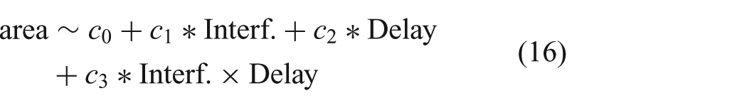
To describe these relationships in a quantitative sense, a mixed-effects model was constructed for the portion of area covered performance metric. Main fixed effects for delay, interface, and prediction horizon were used. An interaction term was included between delay and interface. Other interaction terms were explored, but all had large p-values and thus were not ultimately included in the model presented in Table 3. Finally, each user was treated as a random effect on the intercept to help account for differences in participant skill. The general form of the model was
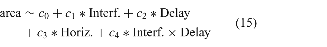
where area is the portion of area covered. Interf. has values 0 representing Interface A and 1 representing Interface B. Delay has values 0 representing 400 ms and 1 representing 800 ms. Horiz. has values 0 representing 0.5 s, 1 representing 1.0 s, and 2 representing 1.5 s.
Mixed-effects model: Portion of area covered (A|B). Delay has the largest impact on portion of area covered. The small mixed effects model coefficient for prediction horizon suggests that there is not a very strong relationship between prediction horizon and portion of area covered.
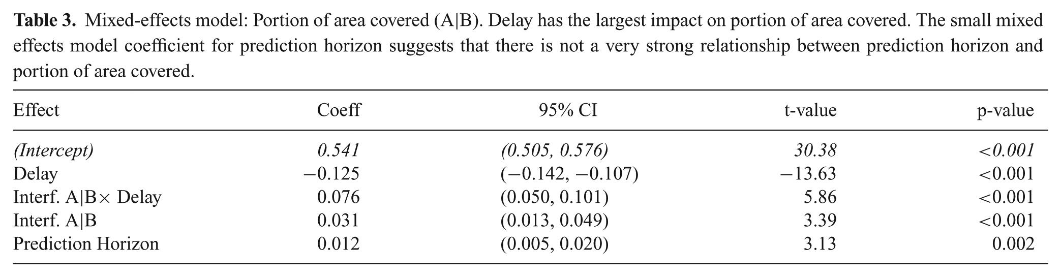
The average area covered and the number of collisions for each interface × delay combination is shown in Fig. 9. The mixed effects model coefficients, their confidence intervals, and statistical significance are displayed in Table 3. Based on Fig. 9 and Table 3, it is evident that delay had the largest impact overall on the portion of area explored. The magnitude of the effect coefficient for delay was four times that of the interface. At the low delay, the shared control mode (Interface B) had a small positive effect on area explored, however the effect is much more pronounced at the higher delay of 800 ms.
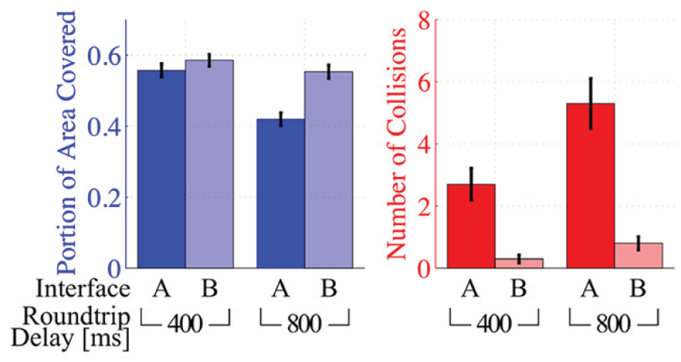
Shared control improved both performance metrics for each interface × delay combination tested in Study 1 but has a more dramatic improvement at the higher delay. The data shown is for a 1.0 s prediction horizon.
From Fig. 9 it is evident that delay and shared control (interface) both had large impacts on the number of collisions. Shared control decreased the number of collisions while increased delay resulted in more collisions. The difference in the number of collisions for each interface at the high delay is larger than the difference at low delay.
One may note that some collisions still occurred even with the shared control (Interface B). This is the result of differences in the model used to solve the model predictive control (MPC) problem and the actual dynamics of the robot. The model used in the MPC problem is a linearized version of the unicycle model with dynamics. The robot operated by users in ANVEL has nonlinear dynamics that include tire friction models, drive motor models, etc. With a better model of the actual robot, there would likely have been fewer collisions. However, the linearized robot model used in the MPC is computationally much more efficient. The differences between the linearized model and ANVEL’s nonlinear model give a more accurate representation of the model inaccuracies that would occur when using a physical robot.
Overall, results from study 1 show that shared control clearly improves safety (fewer collisions) at both low and high communication delays. Performance (in terms of area covered) has a large improvement at high communication delay when adding shared control, but there is little improvement at low delay when adding shared control.
The average area covered and number of collisions for each prediction horizon × delay combination with Interface B is shown in Fig. 10. The mixed-effects model in Table 3 shows that while the effect of prediction horizon on area covered is positive, it is small. In particular the difference between the 0.5 s and 1.5 s prediction horizons was only found to result in a change of about 2.4% more area explored. This trend was similar for the number of OOIs identified.
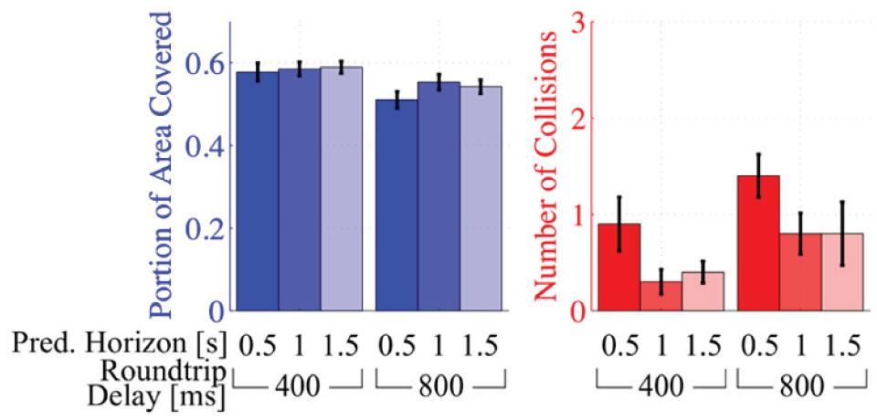
Varying lengths of prediction horizon did not have a large impact on the area covered or the number of collisions at each prediction horizon × delay combination tested in Study 1. However, increasing the prediction horizon from 0.5 s to 1.0 s resulted in fewer collisions. The data shown is for Interface B.
However, the number of collisions does depend on the length of prediction horizon. The number of collisions is higher with the shortest prediction horizon of 0.5 s in comparison to the 1 and 1.5 s horizons. However, the difference in the number of collisions between the 1 and 1.5 s prediction horizons is very small. Overall, prediction horizon has little effect on performance (in terms of area covered), but does have an impact on safety (number of collisions). It appears that beyond a prediction horizon of 1 s, the improvements in safety are very small. The length of the prediction horizon, beyond which safety levels off, likely depends on the dynamics of the robot. That is, a vehicle moving at higher speeds and with lower maximum deceleration capabilities would require a longer prediction horizon.
5.2. User study 2 - Impact of interface and delay
Based on the findings of study 1, we designed and conducted study 2 to investigate Interfaces C-E. From user study 2, three relationships will be highlighted. The first compares interfaces where the user inputs robot velocities versus controlling the position of a steerable waypoint. The second evaluates a navigation interface that has the robot move along Voronoi map paths. The third explores how the location of the shared control method (located on-board the robot versus operator control unit) impacts performance in the presence of communication delay.
For the user study 2 data, mixed-effects models were constructed using main fixed effects for delay and interface. An interaction term was included between delay and interface. Each user was treated as a random effect on the intercept to help account for differences in participant skill. The general form of the model was
where area is the portion of area covered. Interf. has values 0 representing Interface B and 1 representing the relevant Interface C, D, or E. Delay has values 0 representing 400 ms and 1 representing 800 ms.
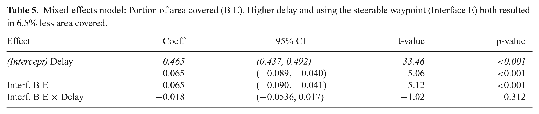
A steerable waypoint interface similar to that used in the military (Metcalfe et al., 2010) and with telepresence robots (Takayama et al., 2011) was tested in study 2. Performance metrics of area and collisions are summarized in Fig. 11 and Table 5. Performance, both in terms of area and collisions, was worse with the steerable waypoint (Interface E) in comparison to subjects controlling the robot’s velocities (Interface B). From the mixed-effects model, one can see that the size of the effects for interface and delay are approximately the same size - 6.5% less area is covered due to the higher delay or due to using the steerable waypoint. The interface × delay coefficient has a high p-value indicating that there was not a significant interaction between communication delay and interface. Decrease in area covered is consistent with the increased task completion times observed in Metcalfe et al. (2010) with the steerable waypoint.
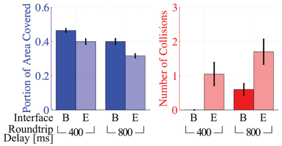
Users performed worse, in terms of area coverage and collisions, at each delay when using the steerable waypoint (Interface E) compared to robot velocity input (Interface B) in Study 2.
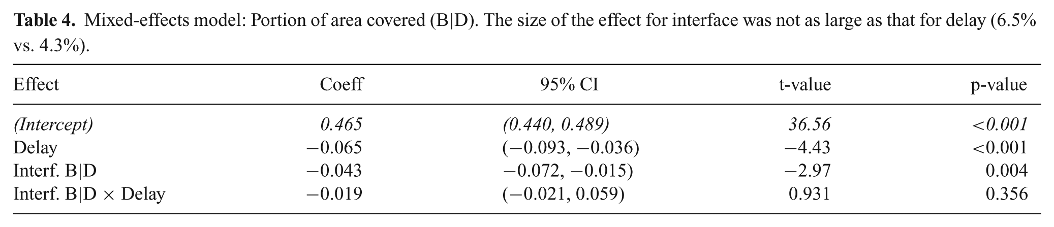
In study 1, it was observed that subjects often tried to maximize their distance from the closest obstacles. When they passed in between obstacles, they often moved along a path that was approximately halfway between the two obstacles. At high communication delays, increasing the distance from obstacles would allow subjects a larger margin for error in navigating without having collisions. Thus, we anticipated subjects would prefer and perform better moving along a Voronoi map. In Interface D, the robot tried to navigate along a Voronoi map around obstacles. Results from study 2, comparing Interfaces B and D, are included in Fig. 12 and Table 4.
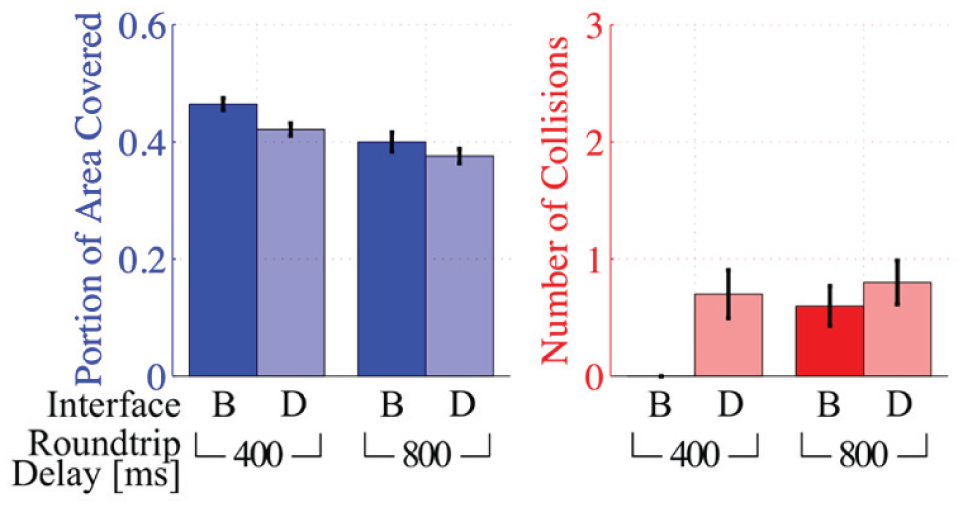
Users performed worse, in terms of area coverage and collisions, at each delay when using the Voronoi map based shared control (Interface D) compared to robot velocity input (Interface B) in Study 2.
Mixed-effects model: Portion of area covered (B|D). The size of the effect for interface was not as large as that for delay (6.5% vs. 4.3%).
Mixed-effects model: Portion of area covered (B|E). Higher delay and using the steerable waypoint (Interface E) both resulted in 6.5% less area covered.
Performance, both in terms of area and collisions, was worse with the Voronoi map based shared control (Interface D) in comparison to subjects controlling the robot’s velocities (Interface B). From the mixed-effects model, one can see that the size of the effect for interface was not as large as that for delay (6.5% vs. 4.3%). The interface × delay coefficient has a high p-value indicating that there was not a significant interaction between communication delay and interface. Additional discussion about the Voronoi map navigation method and possible improvements are presented in Section 6.
In Interface C, the shared control method calculated robot inputs at the operator control station and thus could receive inputs from the human operator without communication delay. However, as described in Section 4.2, the robot state information and control commands sent to the robot were delayed. The resulting interface was more responsive to inputs from subjects (i.e. the robot’s projected path on the screen would update instantly), however actual movement of the robot still felt delayed. Results from study 2 comparing Interfaces B and C are included in Fig. 13 and Table 6.
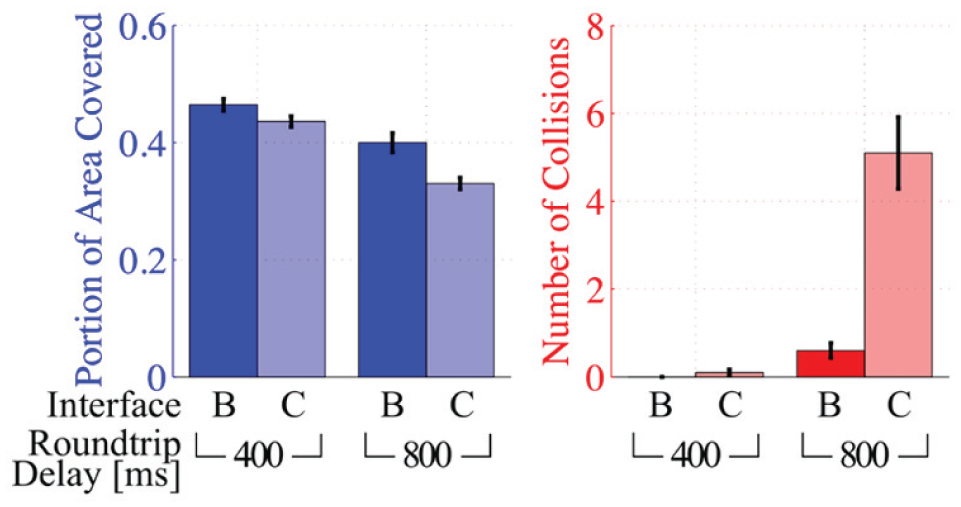
Users performed worse, in terms of area coverage and collisions, at each delay when using Interface C compared to Interface B in Study 2.
Mixed-effects model: Portion of area covered (B|C). The size of the effect for interface was not as large as that for delay (6.5% vs. 2.8%). The size of the effect for Interface C (2.8%) was smaller than the effect size for Interface D (4.3%).
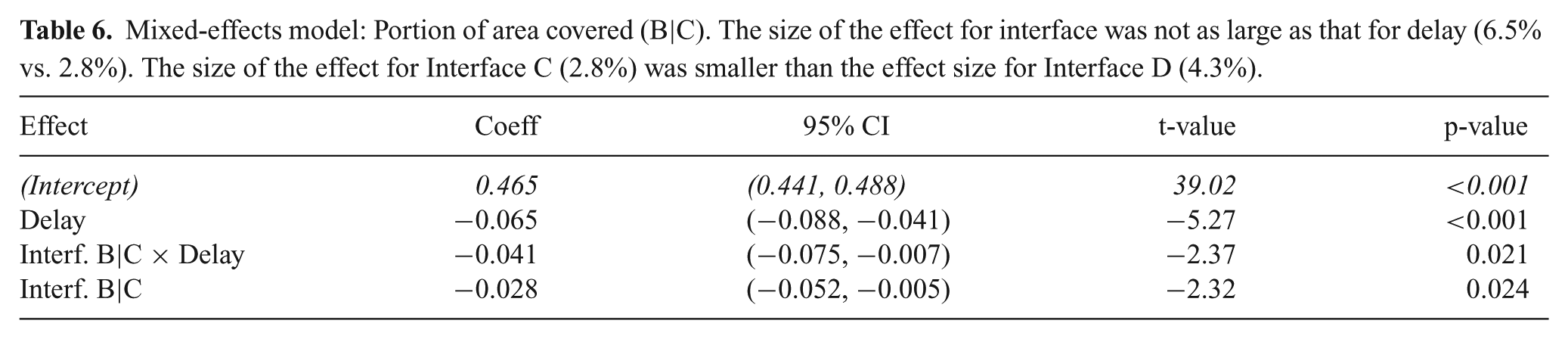
Performance, both in terms of area and collisions, was worse with Interface C than Interface B. From the mixed-effects model, one can see that the size of the effect for interface was not as large as that for delay and was also smaller than the effect size comparing Interface B to D. The interface × delay coefficient has a high p-value indicating that there was not a significant interaction between communication delay and interface. Additional discussion is in Section 6.
Subjective survey results were collected after each test condition. The subjective measures conveyed the same messages, so results for only one of the questions are included in Fig. 14. Subjects responded to the question (shown in the figure title) on a 7-point Likert scale with the ratings described in the legend. Some interesting results can be observed from Fig. 14. First, at low delays the subjective ratings were spread evenly around neutral for Interface E. At the high delay, not a single participant gave a rating of 6 or 7 for Interface E. This disapproval agrees with the objective results that show low area coverage and a higher number of collisions.
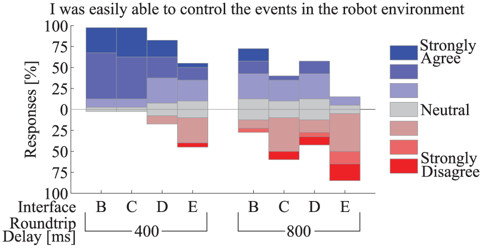
Users felt they were better able to control events in the robot environment best with autonomy located on the operator side (Interface C) at low time delay. However, at higher delay, they preferred having autonomy located on-board the robot and Voronoi map based control (Interfaces B and D, respectively) over autonomy on the operator side (Interface C).
Second, the subjective ratings comparing Interfaces B and D line up well with the objective measures discussed of area coverage and collisions. One can see that number of individuals giving ratings 2-6 on the 7-point scale are nearly identical at the 800 ms delay. The difference in the subjective ratings appears to be at the extremes - more people felt strongly that they could control events with Interface B, while a similar number of people felt strongly that they could not easily control events with Interface D. Third, despite better area coverage with Interface B than C at the 400 ms delay, study participants did not rate Interface B as allowing them to more easily control events in the robot environment. More participants rated “Strongly Agree” for Interface C than for Interface B.
6. Discussion
Results from the two human subject studies demonstrated the effectiveness of the shared control method we developed and identified several key teleoperation relationships. In the discussion that follows, we provide some additional comments/recommendations related to the results for individuals to consider when developing teleoperation systems.
6.0.1. Interaction of shared control and delay
As discussed in Section 2.1, Luck et al. (2006) conducted a study investigating the role of different automation levels and communication delay on performance. In our study, Interface A is most comparable to the teleoperation mode and Interface B is most comparable to the guarded teleoperation mode in Luck et al. (2006). Results from their study show that as delay increases, so do the number of drive errors, and drive errors are lower with guarded teleoperation than regular teleoperation. These results agree with our measurements for the number of collisions.
With regards to the time required to complete the course, results from Luck et al. (2006) show that as the delay increases, so does course completion time and guarded teleoperation is about the same as regular teleoperation. However, we found that the portion of area covered (which compares best to completion time) improves when adding shared control. In fact, we found that with higher delay, the improvement in area coverage is even more pronounced with shared control than at lower delay.
Overall, at low and high time delays our study agrees that adding shared control will decrease drive errors/collisions. Unlike Luck et al. (2006), we also demonstrated that adding shared control provides a larger increase in performance at high delays compared to low delays. We believe the improvement in performance with shared control found in our study is due to the improved formulation of the shared control method presented in Section 3.
6.0.2. Impact of prediction horizon
The prediction horizon used in the shared control method consists of two parts - the time-step size
The results in Fig. 10 and Table 3 suggest that prediction horizon had a small, positive effect on the portion of area covered. With regards to collisions, increasing the prediction horizon from 0.5 to 1 s resulted in fewer collisions. However, increasing the prediction horizon from 1 to 1.5 s had little impact on the number of collisions. Once the prediction horizon is long enough (in our case 1 s), then increasing the prediction horizon has little impact on safety. When selecting length of the prediction horizon for a robotic platform, one should consider the dynamics of the platform. For example, a robot that drives at higher speeds and decelerates slower would require a longer prediction horizon. Additional work is needed to explore how to find the prediction horizon that best balances robot safety and computational requirements.
6.0.3. Control using steerable waypoint
Results in Fig. 11 and Table 4 indicate that the steerable waypoint method performed worse in terms of performance and safety compared to the velocity-input based shared control method in Interface B. Subjective results in Fig. 14 also convey participants’ opinions that control was difficult with Interface E. Many users commented that controlling the steerable waypoint with the gamepad joystick was difficult with the communication delay. The location of the steerable waypoint on the human operator’s screen was responsive; however, the robot’s projected path and movement was still delayed. Perhaps it would have been more intuitive to control the steerable waypoint by using a mouse cursor or using a touch interface (like a tablet computer). We wanted to minimize the number of factors that changed in each comparison (i.e. if performance was better with the steerable waypoint on a tablet in comparison to Interface B, it would have been difficult to determine whether that difference was due to using the steerable waypoint or using the tablet itself). Overall, we do not recommend using a steerable waypoint controlled by a gamepad, joystick or computer keyboard.
6.0.4. Control moving along Voronoi map paths
Voronoi diagrams are very popular in a variety of domains and many efficient methods for constructing them have been developed (Aurenhammer, 1991). Voronoi maps have been used in motion planning for mobile robots to construct paths that reach an end goal while avoiding collisions with obstacles (Takahashi and Schilling, 1989). However, they often have many sharp turns that could create a jagged, unnatural motion for a human operator observing a robot moving along the map. To address this concern, one could move along smoother Bezier curves generated from a Voronoi map (Ho and Liu, 2009). To the best of our knowledge, no prior work has investigated shared control with Voronoi map based navigation.
The results with Voronoi map based shared control (Interface D) in user study 2 show promise, but performance with the robot velocity based input method (Interface B) is better. Subjects did make anecdotal comments that they liked the Voronoi map lines. They said that it was nice to see the possible paths that the robot could follow. However, sometimes the exact direction a subject wanted the robot to move in was not contained on the Voronoi map, or the path to go in that direction was extra long. Subjects also commented that in areas that seemed to be a little bit more densely populated with obstacles, they preferred following the Voronoi map paths.
A number of adjustments could help improve the method. First, using an alternative input device could improve performance. For example, using a mouse or tablet interface to select Voronoi map lines to move along may be a better user interface design and could potentially allow subjects to control multiple robots at once. Second, movement along Voronoi map lines is likely more helpful in densely populated obstacle areas and/or when communication delay is high. Thus, in areas that have few obstacles and low delay, it may be better to have the robot move along a different path, e.g. a minimum time path to another node.
Third, the sharp corners of the Voronoi map around nodes may make the robot movement feel unnatural to human operators. Smoothing the path (especially around nodes) could make the movement feel more natural. Lastly, a better explanation of the path map that the robot is trying to follow could help, given that many operators may not understand Voronoi maps.
6.0.5. Shared control on operator station
We had anticipated that placing the shared control calculations at the operator station would result in an interface with a more responsive feel. However, errors accumulated in the state predictors and control commands were large enough to offset this more responsive feel and cause decreased performance. Study participants’ dissatisfaction with the decreased performance (area coverage) and safety (number of collisions) was also evident in their low subjective ratings of the system in Fig. 14. These results did not agree with our hypothesis that the MPC and model based state predictors could better compensate for the delay than the human operator. In general, we recommend placing autonomous controllers on-board the robot itself, as the user study 2 results suggest that human operators can better compensate for the delay in their inputs, than the robot can for delay in its inputs. Further exploration could be done to look at different predictors.
7. Conclusions
In this paper, we presented a shared control method to aid human operators in robot navigation tasks and avoiding collisions with obstacles. The shared control method builds off previous model predictive control (MPC) formulations and we present a new method of representing obstacle free regions in the MPC problem. The obstacle free region representation makes the method well suited for maneuvering in less structured environments (i.e. environments without roads or paths to follow) and allows the MPC problem to be solved very rapidly. The shared control method was implemented in a realistic robot simulation engine and evaluated with two human subject studies. Results from the user studies showed that performance and safety had small improvements at low communication delay and much larger improvements at high delay with the shared control method. In addition, the user studies explored the impact of control interface and its interaction with communication delay. Delay had the largest impact on performance compared to interface and prediction horizon.
Results from the user studies indicate that human subjects tend to move along Voronoi map lines when the robot is experiencing communication delay and in close proximity to obstacles. Navigation along Voronoi map lines with subjects using a gamepad showed promise, but other input modalities (e.g. mouse, tablet) may be more effective and could be explored in future work. Another area of future work could be to formulate the MPC problem such that preference is given to have the robot move towards areas that have not yet been explored. Overall, if robot designers know a teleoperation system requires a human in the control loop and is going to experience delays on the order of hundreds of ms to 1 s, then it is recommended that they implement shared control on the robot in the remote environment to keep system performance and safety near to that with no delay.
Footnotes
Appendix: Index to Multimedia Extension
Archives of IJRR multimedia extensions published prior to 2014 can be found at http://www.ijrr.org, after 2014 all videos are available on the IJRR YouTube channel at http://www.youtube.com/user/ijrrmultimedia
Sample video of user view with Interface B
Acknowledgements
The authors would like to thank Matt Ko for his assistance setting up the user tests in ANVEL and Justin Crawford for his technical support in ANVEL. The authors would also like to thank Dave Daniszewski, Ben Haynes, Paul Muench, Mitch Rohde, and Steve Rohde for their helpful discussions.
Funding
The author(s) disclosed receipt of the following financial support for the research, authorship, and/or publication of this article: This work was supported by the Automotive Research Center at the University of Michigan, with funding from government contract DoD-DoA W56HZV-14-2-0001 through the US Army Tank Automotive Research, Development, and Engineering Center.