Model-based robocentric planning and navigation for dynamic environments

Abstract

This work addresses a new technique of motion planning and navigation for differential-drive robots in dynamic environments. Static and dynamic objects are represented directly on the control space of the robot, where decisions on the best motion are made. A new model representing the dynamism and the prediction of the future behavior of the environment is defined, the dynamic object velocity space (DOVS). A formal definition of this model is provided, establishing the properties for its characterization. An analysis of its complexity, compared with other methods, is performed. The model contains information about the future behavior of obstacles, mapped on the robot control space. It allows planning of near-time-optimal safe motions within the visibility space horizon, not only for the current sampling period. Navigation strategies are developed based on the identification of situations in the model. The planned strategy is applied and updated for each sampling time, adapting to changes occurring in the scenario. The technique is evaluated in randomly generated simulated scenarios, based on metrics defined using safety and time-to-goal criteria. An evaluation in real-world experiments is also presented.

Keywords

Motion planning dynamic environments robot navigation strategies velocity space

1. Introduction

Applications of autonomous robotic systems are a recognized research priority (e.g. in contexts relating rescue, surveillance, households, guidance, museums, and factories). Robots in these contexts have to coexist or cooperate with humans or other moving vehicles in constantly changing scenarios. Planners for static scenarios and purely reactive avoidance techniques are no longer valid. Motion planning in dynamic scenarios requires being able to predict the future evolution of obstacles, to plan and execute the safest and quickest feasible movements for the robot. Furthermore, kinodynamic constraints must be taken into account to obtain feasible trajectories. In this work we develop a robocentric planning and navigation technique for such environments, which considers safety, manoeuvrability, and constraints on the robot and the environment. The paper offers two main contributions: a new dynamic environment model for non-holonomic robots, which maps the environment on the velocity space of the robot; and a set of planning and navigation strategies, based on the model and on safety and time-to-goal criteria.

In Section 2 the state of the art is presented. In Section 3 the contributions are highlighted and explained. Section 4 establishes the problem to be solved. Section 5 formally defines the dynamic environment model, the dynamic object velocity space (DOVS), and its properties. In Section 6, the decision making, planning and navigation strategies are developed. Section 7 evaluates the method, based on metrics by means of simulations and in real-world experiments. In Section 8 some conclusions and future work are presented.

2. Related work

Motion planning and reactive navigation in static and dynamic environments have been addressed extensively in the literature. Reactive approaches combined with global planning techniques lead to so-called iterative motion planners (e.g. Brock and Khatib, 2000; Fraichard, 1998; Frazzoli et al., 2001; Hsu et al., 2002; Minguez and Montano, 2005; Stachniss and Burgard, 2002). These techniques calculate several steps ahead depending on the time available. The planner evaluates different branches in a tree within a horizon and works out a partial trajectory. This process may be interrupted at any time or is time-bounded to maintain the robot’s reactivity.

Modeling the dynamic environment is a major problem to solve that requires representing the dynamics of the robotic system and the motion evolution of the moving obstacles. Two of the most commonly used and referenced models are the velocity obstacle (VO) (Fiorini and Shiller, 1998), expanded in Shiller et al. (2001), and the inevitable collision states (ICS) introduced by Fraichard and Asama (2003). In VO the set of velocities from the current state that would provoke a collision between a holonomic robot and an obstacle at a time in the future is computed. ICS is directly related to safety.

The non-linear velocity obstacle (NLVO), which is the VO concept applied to obstacles moving along arbitrary trajectories, is used in Large et al. (2002) to compute a risk function from the time to collision to select the best velocity for the robot. An evolved technique that employs the 3D information obtained by the NLVO is presented in Large et al. (2005). The authors developed an iterative approach based on the A* algorithm to incrementally build a solution towards the goal, where real-time issues are also considered. Recently, Kim and Oh (2016) presented a new VO-based approach (OVVO), which improves the velocity selection compared with the VO approach. The method defines a cost function which weighs the similarity to a desired velocity and the level of obstacle avoidance (to move around obstacles to a greater or lesser extent) to decide on the best velocity for the robot in crowded or less-dense scenarios. However, the results are very dependent on weight heuristic parameters.

Regarding safety, LaValle and Kuffner (2001) introduced the concept of region of inevitable collision to identify the states in which there is no control input the robot can apply to avoid a collision. Frazzoli et al. (2001) formulated the concept of $τ$ -safety as a guarantee of no collision during $τ$ seconds for each node of a tree created with a sampling-based algorithm. However, the ICS model focuses on safety by computing the robot states that lead to inevitable collision in a time horizon, for a set of evasive manoeuvres, including the braking manoeuvre.

Fraichard (2007) introduced three safety criteria that a robotic system should consider to compute its future motion, and ICS is presented as a suitable framework to deal with motion safety for motion planning and navigation. Petti and Fraichard (2005), Kalisiak and van de Panne (2007), Chan et al. (2008), and Bekris and Kavraki (2007) exploited an approximation of ICS in different ways. They perform a tree-based search and check for inevitable collision states to provide safety for a time horizon. Martinez-Gomez and Fraichard (2009) presented ICS-Avoid, a reactive navigation approach that selects controls for the robot to move through ICS-free states. Probabilistic versions of ICS were defined in Althoff et al. (2010) and Bautin et al. (2010) to capture the uncertainty about the future behavior of moving objects in real-world situations. Althoff et al. (2012) considered interactions among objects in terms of collision avoidance, reasoning beyond the planning horizon. Bouraine et al. (2012) defined Braking-ICS, a version of ICS that guarantees that if a collision takes place, the robot will be at rest. It was later applied to the development of a partial motion planner by Bouraine et al. (2014).

Shiller et al. (2010) addressed the motion safety issue in the VO framework using the ICS concept for holonomic robots. Calculating the proper time horizon as the minimum time for the robot velocity to exit the velocity obstacle yields a representation of the environment that ensures robot safety as long as the robot velocity does not lie in the velocity obstacle. Seder and Petrovic (2007) adapted the DWA approach (Fox et al., 1997) to consider moving obstacles, which are represented as moving cells in a grid map. Safety is thus considered by computing intersection points between simulated obstacle and robot trajectories in the short term. The cells resulting in collision are marked as forbidden, and a command optimizing a weighted navigation criterion is selected for every sampling time.

Pallottino et al. (2007), Van den Berg and Overmars (2008), Bekris et al. (2009), and Bareiss and Van den Berg (2013), addressed multi-robot systems in which all the agents are capable of making avoidance decisions. They developed coordination schemes to distribute the avoidance actions among the robots. Bareiss and Van den Berg (2015) extended this work, generalizing the reciprocal collision avoidance for robots with different kinematic constraints.

The computation of time-optimal trajectories formulated as a problem of computing time-optimal motions has been explored by several works. Reister and Pin (1994) addressed this problem for a non-holonomic robot with bounded acceleration, in an obstacle-free environment. The authors demonstrated that time-optimal motions are obtained from bang–bang controls (maximum acceleration or deceleration), and parametrize the set of time-optimal trajectories using the switching times. Renaud and Fourquet (1997) computed sequences of extremal controls for acceleration-driven robots to reach time-optimal trajectories in free-space. Balkcom and Mason (2002) focused on differential drive and car-like robots with bounded linear and angular velocities but without acceleration limitations. Shiller et al. (2013) presented an on-line motion planner, where robot dynamics and actuator constraints were considered. A near-time-optimal trajectory that avoids stationary obstacles one at a time is incrementally computed, obtaining comparable results with respect to the global optimal solution. Park et al. (2009) dealt with one moving obstacle, and solved an optimization problem with inequality constraints for a holonomic robot with infinite acceleration. Mercy et al. (2016) formulated the optimization problem in a scenario with moving and static obstacles for a holonomic robot with fixed orientation. Real-time optimization was achieved by a B-spline parametrization of the trajectory and exploiting B-splines properties to limit the set of constraints. A different approach to obtain near-time-optimal trajectories was developed in Gal et al. (2009) and Shiller et al. (2010), which adapt time-optimal solutions based on extremal controls for static or free space environments.

In this paper we develop and evaluate a robot motion planner based on a model which represents the dynamism of the environment. This work extends and formalizes the model of a preliminary work (Owen and Montano, 2005). That work presented the dynamic object velocity (DOV) to model the moving obstacles in the environment, reasoning on it for robot navigation. The DOVS space herein developed explicitly takes into account the future evolution of the obstacles and the dynamics of the robot to compute a set of velocities leading to collision in the future. DOVS is defined upon the concepts of estimated arriving time of the obstacles, used to compute the times to potential collision or escape, and on the maximum and minimum velocities for the robot not to collide. As a consequence, a set of safe and feasible robot velocities is obtained for further planning.

The DOVS model exhibits several differences with respect to the discussed previous works. ICS calculates the states of inevitable collision for a set of escaping manoeuvres, but it does not explicitly compute motion controls for planning motions among the obstacles towards the goals. In addition, the computational cost for several manoeuvres and several objects is high. The VO technique computes states for the next sampling period, including velocity, for which there are collisions with the obstacles; but the planning of collision-free trajectories using this model requires looking ahead, simulating several steps forward. Instead, DOVS explicitly computes safe linear and angular robot velocities (control variables for the robot) which can be applied without collision in a given but not temporally limited horizon, for instance the field of view of the navigation sensors, without requiring several steps of lookahead simulation. In such a way, building DOVS entails an implicit computation of safe velocities (trajectories) without collision within the space horizon established. Moreover, as discussed in Section 5.6, DOVS is not affected by some complexity issues that do apply to those previous techniques.

3. Contributions

The DOVS model implicitly computes a set of collision-free commands for long-term planning within the sensor’s field of view, providing information about collision-free trajectories. A precomputed set of trajectories in the configuration space is represented as sequences of velocity commands in the control space of the robot, which will contain free and forbidden velocities leading to collision, within the space horizon available. Having this greater visibility horizon at the current instant allows the decision process to select the best next motion command from an improved informed search, without needing to simulate the motion several steps ahead. However, only one of these velocity commands is applied for the next sampling period, and a new plan is computed to adapt to new situations in case hypotheses are no longer satisfied.

The contributions are related to two main issues.

Environment modeling mapped on the robot velocity space. The DOVS model is formally defined for different kinds of obstacle trajectories and static obstacles, and its properties regarding safety are established. A complexity analysis of the model and a comparison with respect to other well-known techniques in this field is carried out.

Planning navigation strategies. Using the DOVS model, a strategies-based approach to compute safe motion commands (velocities) for the robot is developed. Navigation decisions are made based on identifying a situation among a discrete set, evaluating the decision variables computed from the model of the environment.

The method is assessed by means of simulations and experiments in real-world scenarios. Randomly selected scenarios and dynamic conditions are used for evaluation. The properties of the model are verified, and metrics for performance evaluation of the navigation strategies are provided.

4. Problem statement

The DOVS model for dynamic environments exploits the concept of estimated arriving time of an object by computing the times of future potential collisions. Then the set of collision-free and collision-causing commands are represented explicitly in the control space of the robot. In such a way, any motion planner based on this model that selects collision-free commands will generate trajectories without collision. To compute the free control space, circular robot trajectories for non-holonomic robots have been selected for the long-term planning. Recomputing the plan every sampling time yields clothoid and anti-clothoid trajectories as the robot moves towards the goal, providing continuous curvature trajectories.

The motion planner applies different strategies of movement depending on the situation of the robot with respect to its environment. The situations are identified from the DOVS model. The decision variables are defined and valued so that a situation is identified and thus a navigation command is computed for that situation.

Robot and obstacle states

We consider a non-holonomic robot $ℛ$ moving in a dynamic environment, where it has to safely reach its goal avoiding collisions with the static and moving objects $O_{i}$ around it. They all share workspace $W S = ℝ^{2}$ . Let $O (t)$ be the set of points in $W S$ occupied by all the obstacles $O_{i}$ at instant $t$ , i.e. $O (t) = \cup O_{i} (t)$ .

The state of the robot is defined by its location and velocity at instant $t$ , $ℛ_{t} = (x y θ ω v)$ . Let $ℛ (v, t)$ denote the state reached by the system $ℛ$ under the action of control $v = (ω, v)$ applied at time $t$ . In our case, the controls are the angular ( $ω$ ) and linear ( $v$ ) velocity for a differential-drive robot. The motion model for the robot can be expressed by the well-known equations:

\dot{x} = v * \cos (θ); \dot{y} = v * \sin (θ); \dot{θ} = ω

(1)

From these states and the motion model we describe the DOVS environment model in the next section.

5. Modeling the environment

The model is constructed by mapping the information from the workspace to the control space of the robot, denominated velocity space ( $V$ ), which is the set of velocities $(ω, v)$ reachable by the robot limited by the maximum and minimum velocity constraints. This space also contains sets of velocities leading to future collision if the robot executes them. In some way these collision velocities represent obstacles mapped into $V$ , so we name them DOV. The space is then used to compute commands without collision for the robot.

The basic concept to build the model is the time of collision between robot and obstacle trajectories. The intersection points are computed from a robocentric representation, resulting in associated information in $V$ of time and velocity that indicate the instants at which an obstacle reaches them, and the velocities for the robot to pass before colliding or after the object passes, avoiding collision. These time–velocity data are then transferred to the control space of the robot to represent the DOV obstacles in the environment, conforming the velocity–time space ( $V T$ ) of the robot. In this work, for the sake of clarity, the method is presented for linear and circular obstacle motion, but other kinds of obstacle trajectories could be used, without loss of generality.

One of the advantages of this technique is that the model maps the safe robot velocities for a space horizon only limited by the field of view of the onboard sensors. This allows motions to be planned at every instant for the whole time horizon corresponding to the space horizon and not only for the next sampling period in a purely reactive way. Hence, this approach does not need to simulate future trajectories (states) to obtain a long-term plan, as most of the techniques previously referenced do. In addition, owing to computational burden or to practical navigation issues, this space horizon could be artificially limited, enabling reasoning about the behavior of only the closest obstacles, which are those that will impose the immediate manoeuvring decisions.

5.1. The DOVS

In this section the DOVS is defined and its properties described. Appendix B contains the equations for computing the model for linear and circular obstacle trajectories together with a more detailed explanation of the computation process. Next, a brief description is provided.

The model results from computing the times of collision between different feasible robot trajectories and obstacle trajectories in a robocentric reference. Figure 1(a)–(c) demonstrate this idea. In Figure 1a the workspace at a specific instant is depicted. The information in the workspace is mapped to a robocentric representation (Figure 1(b)) to $V$ (Figure 2(b)). The robot is reduced to a point and the obstacles are enlarged with the radius of the robot. They are modeled as wrapping squares. It is also assumed that the future trajectory of each obstacle $O_{i}$ is known or estimated.

Fig. 1.

(a) Workspace; (b) collision band swept by object $O_{i}$ , object $O_{i}$ in positions $O_{i}^{1}$ and $O_{i}^{2}$ , path $γ_{j}$ , and collision points $P_{1 j}$ and $P_{2 j}$ in the robocentric ( $R$ ) configuration space; (c) multiple paths $Γ$ through the collision band.

Fig. 2.

(a) Velocity–time space DOVTS and velocity–time obstacle DOVT; (b) projection of DOVTS on the plane $(w, v)$ , DOVS, and DOV (projection of DOVT).

In Figure 1(b) the $C ℬ_{i}$ (collision band) swept by an enlarged obstacle $O_{i}$ moving in a straight line is depicted. A circular trajectory $γ_{j}$ for the robot is also shown. Let $Γ$ be a discretized set of feasible circular trajectories covering the whole range in $W S$ (see Figure 1(c)). Then $γ_{j} \in Γ$ .

Let $P_{1 j}$ and $P_{2 j}$ be the intersection points between $γ_{j}$ and the outline of $C ℬ_{i}$ . These points represent the collision points in $W S$ between $ℛ$ and $O_{i}$ , and will determine the opportunities for the robot to pass before ( $P_{2 j}$ ) or behind the obstacle ( $P_{1 j}$ ) by following trajectory $γ_{j}$ . Then, the times at which the obstacle reaches those points, $O_{i}^{1}$ and $O_{i}^{2}$ , respectively, are computed. These times are the estimated arriving times of the object, which indicate times of collision. Thus, the minimum and maximum velocities that allow the robot to pass before or after the obstacle, respectively, are

\begin{array}{l} ω_{k j} = \frac{θ_{k j}}{t_{k j}} = \frac{atan 2 (2 x_{k j} y_{k j}, x_{k j}^{2} - y_{k j}^{2})}{t_{k j}} \\ v_{k j} = r_{j} ω_{k j}, k = 1,2 \end{array}

(2)

where $θ_{k j}$ is the angular displacement on $γ_{j}$ for the robot to reach $P_{k j} = (x_{k j}, y_{k j})$ , $k = 1 . . 2$ . See Appendix B for details.

These calculations are extended to the whole set $Γ$ (Figure 1(c)). The computed velocities and times to collision for $Γ$ are mapped in the velocity–time space. Figure 4(a) shows the $V T$ space of the robot including the resultant velocities and times of collision. These sets correspond to the limits of dynamic object velocity–time (DOVT), and the corresponding DOV in $V$ (Figure 2(b)), which will be defined formally later. The velocities in between are forbidden because they lead to a collision with the obstacle at some time, so any velocity outside DOVT can be chosen as a safe command. In Figure 3, the robocentric representation of an obstacle following a circular trajectory and its corresponding DOV are plotted.

Fig. 3.

(a) Robocentric representation of an obstacle circular trajectory (blue) and a set of circular trajectories for the robot (green). (b) The corresponding model in DOVS.

As a first approach, to simplify the model management, we propose to use the projection of the 3D space $V T$ into $V$ , represented in Figures 2(b) and 3(b). Note that the circular paths are transformed in this plane into straight lines, with slope $γ_{j} = v_{m_{j}} / w_{m_{j}}$ , $γ_{j} \in Γ$ , as shown in Figure 2(b). In this figure, the extreme velocities correspond to $v_{1 j} = (ω_{1 j}, v_{1 j})$ , maximum robot velocity leading to collision, and $v_{2 j} = (ω_{2 j}, v_{2 j})$ , minimum velocity to escape from collision, for the path $γ_{j}$ .

We now formally define the space for the robot and its characteristic variables.

Definition 1 (Dynamic object velocity–time). The dynamic object velocity–time ( $D O V T$ ) for a particular moving object $O_{i}$ with respect to the set of feasible trajectories of the robot $Γ$ is defined as the set of velocities that produce a collision with $O_{i}$ at time $t$ ,

\begin{array}{l} D O V T (O_{i}, Γ) = {(ω, v, t) \in V \times ℝ | \exists γ_{j} \in Γ, \\ \frac{v}{ω} = γ_{j}, v_{j} = (ω, v), ℛ (v_{j}, t) \cap O_{i} (t) \neq \emptyset} \end{array}

(3)

Definition 2 (Dynamic object velocity). The dynamic object velocity ( $D O V$ ) for a particular moving object $O_{i}$ with respect to the set of feasible trajectories $Γ$ is defined as the projection of its $D O V T$ , i.e. the set of velocities that produce a collision with $O_{i}$ at any time,

\begin{matrix} D O V (O_{i}, Γ) = {(ω, v) \in V | \exists γ_{j} \in Γ, \frac{v}{ω} = γ_{j}, \\ \exists t \in ℝ, v_{j} = (ω, v), ℛ (v_{j}, t) \cap O_{i} (t) \neq \emptyset} \end{matrix}

(4)

Accordingly, we define $D O V T (O, Γ)$ and $D O V (O, Γ)$ (henceforth $D O V T$ , $D O V$ ) with respect to all the obstacles in the environment,

D O V T (O, Γ) = \cup_{O_{i}} D O V T (O_{i}, Γ)

(5)

D O V (O, Γ) = \cup_{O_{i}} D O V (O_{i}, Γ)

(6)

Definition 3 (Free velocity). The free velocity ( $F V$ ) is the set of velocities outside $D O V$ ,

\begin{array}{l} F V = {(ω, v) \in V | v_{j} = (ω, v) \notin D O V, \forall t \in ℝ, \\ ℛ (v_{j}, t) \cap O (t) = \emptyset} \end{array}

(7)

Velocities belonging to DOV are unsafe, leading to collision at some future time. Any velocity inside $F V$ will be safe in the long term, given that the initial conditions remain.

Definition 4 (Dynamic object velocity space). The dynamic object velocity space (DOVS) is defined as the control space of the robot which contains controls belonging to $D O V$ and $F V$ ,

D O V S = {D O V \cup F V}

(8)

Given that the navigation method presented in this paper focuses on projection DOVS, the definitions which follow are provided only with respect to DOVS. However, they are straightforwardly applicable to $D O V T S$ . Now, we introduce characteristic sets from DOVS.

Definition 5. Let $V_{l o w}$ and $V_{h i g h}$ respectively be the set of maximum and minimum velocities computed for all paths in $Γ$ (Figure 2b),

\begin{array}{l} V_{l o w} (O_{i}, Γ) = {(ω, v) \in D O V (O_{i}, Γ) | v_{j} = (ω, v) = v_{1 j}, \\ t = t_{1 j}, ℛ (v_{j}, t) \cap O_{i} (t) \neq \emptyset} \end{array}

(9)

\begin{array}{l} V_{h i g h} (O_{i}, Γ) = {(ω, v) \in D O V (O_{i}, Γ) | v_{j} = (ω, v) = v_{2 j}, \\ t = t_{2 j}, ℛ (v_{j}, t) \cap O_{i} (t) \neq \emptyset} \end{array}

(10)

Note that $V_{l o w}$ and $V_{h i g h}$ represent the contour of the $D O V$ for a particular object, i.e.

\begin{array}{l} (ω, v) \in V_{l o w} (O_{i}, Γ) \leq (ω, v) \in D O V (O_{i}, Γ) \\ \leq (ω, v) \in V_{h i g h} (O_{i}, Γ) \end{array}

(11)

Definition 6. Let $V_{d o w n}$ , $V_{u p}$ and $V_{s i d e}$ be the sets of velocities in $F V$ eligible for the robot to move safely. In Figure2(b), they represent the velocity commands under $V_{l o w}$ , above $V_{h i g h}$ , and below the bounds of $D O V$ , respectively. Let $γ_{l}$ and $γ_{r}$ be the left most and right most radius shaping $D O V$ in DOVS :

\begin{matrix} V_{d o w n} = {(ω, v) \in F V | \forall γ_{j} \in Γ, \frac{v}{ω} = γ_{j}, \\ v_{j} = (ω, v) < v_{1 j}, \forall t \in ℝ, ℛ (v_{j}, t) \cap O (t) = \emptyset} \end{matrix}

(12)

\begin{matrix} V_{u p} = {(ω, v) \in F V | \forall γ_{j} \in Γ, \frac{v}{ω} = γ_{j}, \\ v_{j} = (ω, v) > v_{2 j}, \forall t \in ℝ, ℛ (v_{j}, t) \cap O (t) = \emptyset} \end{matrix}

(13)

\begin{matrix} V_{s i d e} = {(ω, v) \in F V | \forall γ_{j} \in Γ, \frac{v}{ω} = γ_{j} \notin [γ_{l}, γ_{r}], \\ v_{j} = (ω, v), \forall t \in ℝ, ℛ (v_{j}, t) \cap O (t) = \emptyset} \end{matrix}

(14)

From these definitions we can obtain some important properties that must be used by any planner based on this model to select safe robot commands ensuring collision avoidance in a dynamic environment.

Property 1. Selecting velocity commands in $V_{d o w n}$ yields no collision trajectories. Formally,

\forall v_{j} \in V_{d o w n} \Rightarrow ℛ (v_{j}, t) \cap O (t) = \emptyset, \forall t \in ℝ

Proof. By the definition of $V_{d o w n}$ , if $v_{j} \in V_{d o w n}$ , then $v_{j} < v_{1 j}$ , where $γ_{j} = \frac{v_{j}}{w_{j}} = \frac{v_{1 j}}{w_{1 j}}$ . Then, $\exists t \in ℝ$ such that $ℛ (v_{j}, t) = P_{1 j}$ , the intersection point with the collision band. Given that $v_{j} < v_{1 j}$ , then $t > t_{1 j}$ . At time $t$ the object has passed $P_{1 j}$ , and a collision cannot be produced on $γ_{j}$ .

Property 2. Selecting velocity commands in $V_{u p}$ yields no collision trajectories. Formally,

\forall v_{j} \in V_{u p} \Rightarrow ℛ (v_{j}, t) \cap O (t) = \emptyset, \forall t \in ℝ

Proof. By the definition of $V_{u p}$ , if $v_{j} \in V_{u p}$ , then $v_{j} > v_{2 j}$ , where $γ_{j} = \frac{v_{j}}{w_{j}} = \frac{v_{2 j}}{w_{2 j}}$ . Then, $\exists t \in ℝ$ such that $ℛ (v_{j}, t) = P_{2 j}$ , the intersection point with the collision band. Given that $v_{j} > v_{2 j}$ , then $t < t_{2 j}$ . At any time before $t_{2 j}$ the object has not yet arrived at $P_{2 j}$ , and a collision cannot be produced on $γ_{j}$ .

Property 3. Selecting velocity commands in $V_{s i d e}$ yields no collision trajectories. Formally,

\forall v_{j} \in V_{s i d e} \Rightarrow ℛ (v_{j}, t) \cap O (t) = \emptyset, \forall t \in ℝ

Proof. If $v_{j} \in V_{s i d e}$ , then $\frac{v_{j}}{w_{j}} = γ_{j} \notin [γ_{l}, γ_{r}]$ , by the definition of $V_{s i d e}$ . Thus, no collision could be produced as the resultant trajectory $γ_{j}$ does not intersect the bounds of the $C ℬ_{i}$ at any time.

Property 4. Selecting velocity commands in $D O V$ yields collision trajectories. Formally,

\forall v_{j} \in D O V \Rightarrow \exists t \in ℝ, ℛ (v_{j}, t) \cap O (t) \neq \emptyset

Proof. If $v_{j} \in D O V$ , then $v_{j} > v_{1 j}$ and $v_{j} < v_{2 j}$ , by the definition of $D O V$ . Then, $\exists t_{1}, t_{2} \in ℝ$ such that $ℛ (v_{j}, t_{1}) = P_{1 j}$ and $ℛ (v_{j}, t_{2}) = P_{2 j}$ . Given that $v_{j} > v_{1 j}$ , then $t_{1} < t_{1 j}$ , which means that at time $t_{1}$ the object is still at $P_{1 j}$ and a collision is produced. Likewise, given that $v_{j} < v_{2 j}$ , then $t_{2} > t_{2 j}$ , which means that at time $t_{2}$ the object has already reached $P_{2 j}$ and a collision is produced. Then, a collision could be produced sometime within the interval $t \in [t_{2 j}, t_{1 j}]$ .

Summarizing the properties, when a velocity command is chosen out of $D O V$ , collision avoidance is guaranteed as long as the command is maintained and the object motion hypotheses are met. Thus, commands can be safely changed every sampling control period, as long as they remain outside $D O V$ . In the event that a sudden unforeseen change of an object motion results in the current velocity being inside a $D O V$ , it still could be possible, time permitting, to escape collision by correctly choosing subsequent velocity commands. This is illustrated in examples in Section 6.

5.2. Dealing with multiple objects in DOVS

Figure 4 shows a situation with two objects in $W S$ , DOVTS and DOVS. In the DOVTS space, moving objects are represented as their corresponding DOVT surfaces. Clearly, the highest surface in Figure 4(b) corresponds to the farthest or the slowest object with respect to the robot, and the lowest surface to the nearest or the quickest obstacle. Working directly in DOVTS would allow to utilize the velocity–time room between both surfaces for manoeuvring among the objects. Figure 4(c) shows the projection of both surfaces in DOVS. When this space is used to plan trajectories, the DOV objects can be geometrically merged to obtain one compound DOV object (Figure 4(d)). Reasoning in this space to compute the motion commands in the free velocity space ( $F V$ ) is now made using the merged object, directly exploiting the same properties introduced above. This leads to more conservative navigation decisions than if the whole DOVTS was used, which is one of the objectives for future work.

Fig. 4.

(a) A situation with two moving objects near to each other in $W S$ . (b) The situation represented in DOVTS. (c) Projection of both moving objects in DOVS. (d) The merged DOV object.

5.3. Static objects in DOVS

Static obstacles can also be represented in DOVS. Let $D_{s a f e}$ be the displacement the robot requires on a path to reach zero speed from its current velocity. If the distance to a static object is greater than $D_{s a f e}$ , then the circular path in DOVS is mapped as free of collision. Otherwise, the maximum velocity that the robot should have to stop before a collision, $v_{s t o p}$ , is calculated and mapped into DOVS. Any higher velocity is mapped as a collision one. Figure 5 depicts the result of mapping a static corridor-like object into DOVS.

Fig. 5.

(a) Mapping a corridor into DOVS. The red points correspond to scan laser points for example and the green points are the points after extending the walls with the robot radius. (b) The corridor mapped into DOVS showing the maximum velocity reachable for the robot on each circular path considered.

5.4. The kinodynamic constraints in the model

The maximum linear and angular velocity constraints are explicitly represented in DOVS by the external square (omnidirectional robot) or the external rhombus (differential drive robot) in Figure 6. So far, it has been assumed that any $v_{o}$ could be reachable in one sampling step from the current velocity, which depends on the robot’s maximum acceleration. The dynamic constraints of the robot define the velocity window ( $V W$ ) centered in its current velocity $v_{c}$ and bounded by the acceleration constraints ( $a_{m}, α_{m}$ ). That is, $(v_{c} \pm a_{m} Δ t, w_{c} \pm α_{m} Δ t)$ , the inner rectangle and rhombus in Figure 6(a) and (b), respectively. The shape of this window also represents the kinematic constraints corresponding to the type of the robot model.

Fig. 6.

Kinodynamic constraints in DOVS : (a) holonomic robot, $v_{o}$ is reachable only inside $V W$ , a square window; (b) non-holonomic robot, $v_{o}$ is not reachable within $V W$ , a rhombus window. Circular, clothoid, and anti-clothoid trajectories in DOVS are shown in red. Here $R_{n e w_g o a l}$ represents a new radius, computed in the free zone, to be followed until the true $R_{g o a l}$ becomes free.

Figure 6(a) shows that $v_{o}$ can only be reached in one step from the velocities inside $V W$ , due to the dynamic constraints. In Figure 6(b) it can be seen that $v_{o}$ cannot be reached in one step from $v_{1}$ . To deal with this problem, we compute first the number of sampling periods needed to reach the limits $V_{l o w}$ and $V_{h i g h}$ from the current velocity in DOV, adding them to $t_{l o w}$ and $t_{h i g h}$ to obtain $t_{l o w}^{'}$ and $t_{h i g h}^{'}$ , respectively. These times are used to recompute the new velocity limits $(V_{l o w}^{'}$ , $V_{h i g h}^{'})$ using Equations (2).

5.5. Trajectories in DOVS

Different kinds of trajectories can be selected to execute the motion plan and manoeuvre the robot. In this work we consider bounded velocity and acceleration for real robots, and apply extremal actions (maximum acceleration or deceleration) motivated by results presented in Reister and Pin (1994), introduced in Section 2. As described in previous work by Owen and Montano(2005), this type of control action yields rectilinear, clothoid (only angular acceleration), and anti-clothoid (only linear acceleration) paths, allowing a curvature continuity. Moreover, as shown in Section 5.1, circular and linear trajectories are also used for motion planning and execution.

These mentioned trajectories are directly mapped on DOVS (see Figure 6b). Linear trajectories in the workspace appear as a straight line in the $v$ axis ( $ω = 0$ ). Circular paths are mapped as straight lines with a slope, which represent different radii ( $γ = v / ω$ ) ( $v_{3}$ – $v_{4}$ red line). Clothoids are depicted as straight horizontal lines ( $v = c o n s t a n t$ ) ( $v_{2}$ – $v_{3}$ red line), and anti-clothoids as vertical lines ( $ω = c o n s t a n t$ ) ( $v_{1}$ – $v_{2}$ red line).

5.6. Complexity of modeling and planning algorithms

A comparison is performed to analyze the complexity of the algorithms presented for modeling the dynamic environment and its use for planning in other techniques proposed in the literature, specifically those based on VO and ICS, with respect to our proposal.

Computing the set of ICS of a robot for different control trajectories and several obstacles involves a complexity of $O (m n t_{m a x} o)$ , where $m$ is the number of obstacles, $n$ the number of evasive manoeuvres, $t_{m a x}$ a lookahead for practical use of the approach and $o$ the sum of vertices of the robot and the most complex object, which are involved in the Minkowski difference operation required between each robot–obstacle pair. Parameter $t_{m a x}$ is the number of sampling periods, with a duration of $Δ t$ each, considered for computing the ICS set, and thus the total time of such states being ICS. It is assumed that the workspace is bounded, and the robot and obstacles will exit it at $t_{m a x}$ . By using graphics processing unit (GPU) the complexity can be reduced to $O (m n t_{m a x})$ (see Martinez-Gomez, 2010).

The VO approach concerns mainly three operations: computing each individual ${VO}_{j}$ for $j = 1 . . m$ obstacles, the multiple velocity obstacle MVO, and the set of safe velocities. The most complex operation is the second one, because it requires updating the points of each ${VO}_{i}$ , $i = j + 1 . . m$ , with the intersection points between ${VO}_{j}$ and each ${VO}_{i}$ , and ordering them clockwise, which leads to a complexity of $O (m^{2})$ . This can be reduced to $O (m \log m)$ by storing the points within a more efficient structure (see Fiorini, 1995). However, this approach provides information only for computing the next control command as constrained to the acceleration window. If a further plan has to be obtained, a tree search would be performed expanding the nodes for the lookahead considered $t_{m a x}$ , which has the same meaning as in ICS. Then, the complexity would be $O (q^{t_{m a x} / Δ t} m \log m)$ , where $q$ is the fixed number of velocities that can be reached within the next sampling period, and $t_{m a x} / Δ t$ represents the number of levels achieved during tree expansion.

In our technique, the complexity of modeling each moving object in its ${DOV}_{j}$ , $j = 1 . . m$ , is $O (m n)$ , where $m$ is the number of obstacles and $n$ the maximum number of the trajectories considered ( $Γ$ ). The set of trajectories selected for computing a ${DOV}_{j}$ depends on the position of the obstacle and its motion with respect to the robot, and on the desired discretization. The calculation for collision times and forbidden velocities is therefore focused on the area where the obstacle will be moving. Thus, several robot trajectories are considered for each obstacle. Furthermore, the complexity for mapping objects moving in linear and non-linear trajectories (in particular, circular paths have been developed in this work) is the same, because only intersection points with the collision band are needed, not altering the computation burden. The approach presented in this paper deals with multiple objects by merging all ${DOV}_{j}$ . This operation requires for an object to compute the collision times and velocities for the robot trajectories considered for the other objects, and to repeat this for each object. The complexity is then $O (n m^{2})$ . This approach provides enough information for computing plans in the defined workspace horizon, so the complexity is not affected by the parameter $t_{m a x}$ of the other methods, since a lookahead simulation is not needed for planning safe motions. In Section 6.2 the criteria to select near time-optimal actions are explained.

6. Decision making for planning and navigation

This section explains the decision-making process for a robot when dealing with moving obstacles. The problem is similar to a situation in which a pedestrian intends to cross a road while cars are passing. The pedestrian must decide how to do this safely. In such a situation, the main decision the robot must take is whether to pass before or after the obstacle.

Most of the proposed techniques for navigation in dynamic environments limit the number of possible robot trajectories or manoeuvres, or simply slow down or stop the robot to avoid a collision by allowing the moving obstacle to pass first. The method presented in this work enables lighter computation of long-term safe command sequences in the free-velocity space, and thus the corresponding trajectories to the goal. These planned trajectories are not time-optimal, but are used as a first seed to guide the robot towards the goal in the free space. In the following steps, the recomputed extremal control commands will lead the robot to move in near time-optimal trajectories to the goal.

The design is based on the paradigm of situated activity (Arkin, 1998). The robot decides the motion plan within a set of finite but general situations identified from the perception system. Each situation has an associated motion strategy, which exploits the information provided by the model of the environment. Two main criteria are considered to define the strategy: (i) the trajectories generated have to be safe; (ii) near-time-optimal trajectories to the goal have to be generated. The first is ensured by selecting velocity commands inside the free velocity $F V$ of the control space, as explained in the previous section. The second criterion is accomplished by the strategies defined for each situation, computing velocity commands complying with the robot kinodynamic constraints. Each motion leads to a stretch of trajectory, which combined during navigation drive the robot to the goal maintaining the highest velocities possible.

Figure 7 reflects this idea. Essentially, there are two main planning decisions: passing before the object ( $R o b o t F r o n t$ ) and passing after the object ( $R o b o t B e h i n d$ ). In turn, each is decomposed into different sub-decisions depending on whether the robot is before, inside or after the collision band. The execution of each motion strategy depends, in turn, on several decision variables, which drive the hierarchical decision process implemented in a decision tree. These variables are formally defined in the next subsection.

Fig. 7.

Trajectory in green when the robot passes before the moving obstacle and in red when the robot passes after the moving obstacle.

6.1. Decision variables

Table 1 summarizes the decision variables, some in the workspace $W S$ and others in DOVS, including a brief explanation about their meaning and their use in the different situations. An important decision variable is $G D$ (goal direction), which maps a circular trajectory from the current robot location towards the goal. If this trajectory is followed, reaching the goal is ensured. Commands always have to be selected in $F V$ (free velocity) space. Then, when $G D$ lies inside a DOV, it has to be moved to $F V$ ( $G D_{n e w}$ in Figure 8(a)). To that end, a nearby velocity sub-goal that avoids the obstacles, not only in the next sampling period but also within the visibility horizon, is chosen. Figure 8(b) shows a situation in which there are not $U p p e r F r e e$ velocities, so only $V_{d o w n}$ and $V_{s i d e}$ velocities can be selected.

Table 1.

Decision variables in WS and DOVS.

Variable	Meaning	Situation
WS
$R e l P o s$	relative position before, in, or after the collision band	all
$A n g D i s$ ( $θ_{m}$ )	angular distance robot–goal	all
DOVS
$F V$ - DOV	free ( $F V$ ) and non-free (DOV) velocities	all
$V_{h i g h}$	minimum velocities to pass before object	PassingBefore, SlowingDown
$V_{l o w}$	maximum velocities to give way to object	PassingBefore, SlowingDown
$V_{u p}$ - $V_{d o w n}$	high ( $v > V_{h i g h}$ ) - low ( $v < V_{l o w}$ ) free velocities	all
$V_{s i d e}$	free velocities $v = {(ω, v) \| \frac{v}{w} = γ_{j} \notin [γ_{l}, γ_{r}]}$	all
$v_{v a l l e y}$	${(ω, v)}_{v a l l e y} = \min (V_{h i g h})$	PassingBefore
$U p p e r F r e e$	free angular velocities with maximum linear velocity	PassingBefore, PassingAligned
$S a f e V e l$	safe low velocities to avoid or escape from collision	SlowingDown
$B o u n d R i g h t$ – $B o u n d L e f t$	$γ_{r}$ – $γ_{l}$ mapped in velocity space, boundaries for $V_{s i d e}$	AvoidingObject
$v_{m}$ , $ω_{m}$ , $a_{m}$ , $α_{m}$	maximum linear and angular velocities and accelerations	all
$V W$ (velocity window)	velocities that can be reached within next time interval	all
$G o a l D i r e c t i o n (G D)$	${(ω, v)}_{G D}$ mapped direction in velocity space	all
$S t e e r i n g D i r (S D)$	$ω_{S D}$ mapped angular deviation to goal in velocity space	all

Fig. 8.

Decision variables in DOVS. (a) Situation in which there are $U p p e r F r e e$ velocities (magenta, blue, and pink); given that $G D$ lies inside the DOV, the closest $U p p e r F r e e$ to $G D$ will be chosen, computing $G D_{n e w}$ . (b) Situation in which $U p p e r F r e e$ is occupied with velocities leading to collision (gray), only low velocities in $V_{d o w n}$ and $V_{s i d e}$ can be selected.

6.2. Optimization based on decision variables

The decision-making process described above is implemented by means of navigation strategies, which use the defined decision variables. The objective of the strategies is to navigate towards the goals in dynamic scenarios, executing near-time-optimal trajectories whilst ensuring safety (no collisions). Unlike in static environments, in dynamic environments where obstacle motion is uncertain or it might unexpectedly change, computing global time-optimal trajectories is not feasible.

To apply the decision-making strategies based on DOVS model, the direction to the goal is projected in DOVS as the decision variable $G D$ , representing a steering direction that drives directly to the goal, planning initially a circular trajectory $γ_{G D}$ from the current robot location. This trajectory is not time-optimal, so it will only serve as an initial reference to move towards the goal. Two kinds of extremal controls are chosen to be applied every sampling time to reach $G D$ , either maximum angular acceleration to optimally align first the robot to goal position, or maximum linear acceleration for optimally approaching the goal. This kind of trajectories were derived in Reister and Pin (1994) as time-optimal ones for differential-drive robots with acceleration constraints in free space. We have adapted that technique for dynamic environments, obtaining near-time-optimal trajectories. They lead to clothoid and anti-clothoid trajectories, respectively (see Figure 9(a) and (b)). Moreover, we have to take into account the kinodynamic constraints of the vehicle, which limit the acceleration and the velocity to be applied during every control sampling time.

Fig. 9.

(a) Clothoid and (b) anti-clothoid trajectories for different initial values of $ω_{0}$ . The higher $ω_{0}$ , the quicker the aligning to the goal. (c) Times to goal $t_{G}$ for trajectories in (a) and (b). (d) Time to goal difference $t_{G}$ (clothoid) $- t_{G}$ (anticlothoid) for different goal distances ( $d$ ) and angular deviations ( $a n g$ ) with high and low maximum linear velocities.

The time-to-goal for a clothoid, $t_{G_{w}} (v_{c}, θ_{m}, d_{G})$ , and for an anti-clothoid, $t_{G_{v}} (v_{c}, θ_{m}, d_{G})$ , depends on several decision variables. Since these trajectories are computed from Fresnel functions, which analytic solution cannot be obtained for all the decision variables, we have analyzed by simulation both time functions ( $t_{G_{w}}, t_{G_{v}}$ ) for different $ω_{0}$ initial conditions. In Appendix C, these functions are described. Figure 9 represents them. The conclusion of this study is that for an ample range of $ω_{0}$ and for near and far goals the clothoids result in lower times, mainly for low values of $ω_{0}$ . Thus, it can be deduced that it is always better initially to increase the angular velocity up to the maximum if possible, rather than keeping the initial angular velocity, until an angular deceleration is needed for aligning. When the robot is nearly aligned to the goal, a linear acceleration is applied to speed up to maximum velocity. Algorithm 6.2 implements this method, and is used in the strategies to avoid moving obstacles.

Algorithm 1 Align the robot to the goal
Require:
1: $v_{c}$ , the current velocity of the robot
2: ${(ω, v)}_{G D}$ , maximum velocity to goal direction in DOVS
3: $θ_{m}$ , angular deviation to goal from current robot position
4: $d_{G}$ , distance to goal from current robot position
5: function Aligning( $v_{c}$ , ${(ω, v)}_{G D}$ , $θ_{m}$ , $d_{G}$ )
6: if $\| ω_{c} \| \neq \| ω_{G D} \|$ then
7: ▷robot not aligned (clothoid)
8: $ω_{i} = {argmin}_{v \in V W} (t_{G_{w}} (v_{c}, θ_{m}, d_{G})) =$
9: $= {argmin}_{v \in V W} (w_{m} - ω_{G D})$
10: $v_{i} = v_{c}$
11: else ▷robot is aligning (anti-clothoid)
12: $ω_{i} = ω_{c}$
13: $v_{i} = {argmin}_{v \in V W} (t_{G_{v}} (v_{c}, θ_{m}, d_{G})) =$
14: $= {argmin}_{v \in V W} (v_{c} - v_{G D})$
15: end if
16: return $(ω_{i}, v_{i})$
17: end function

6.3. Situation-based navigation

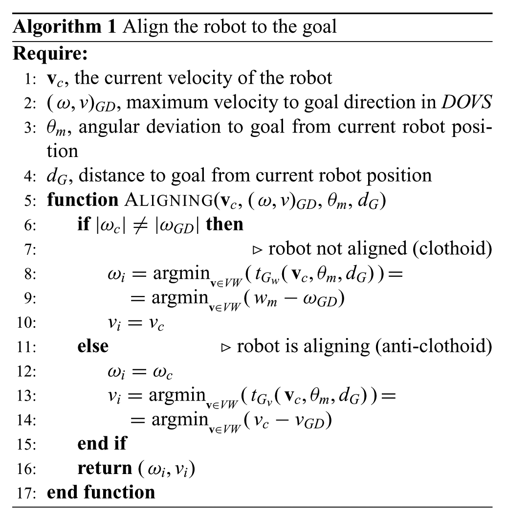
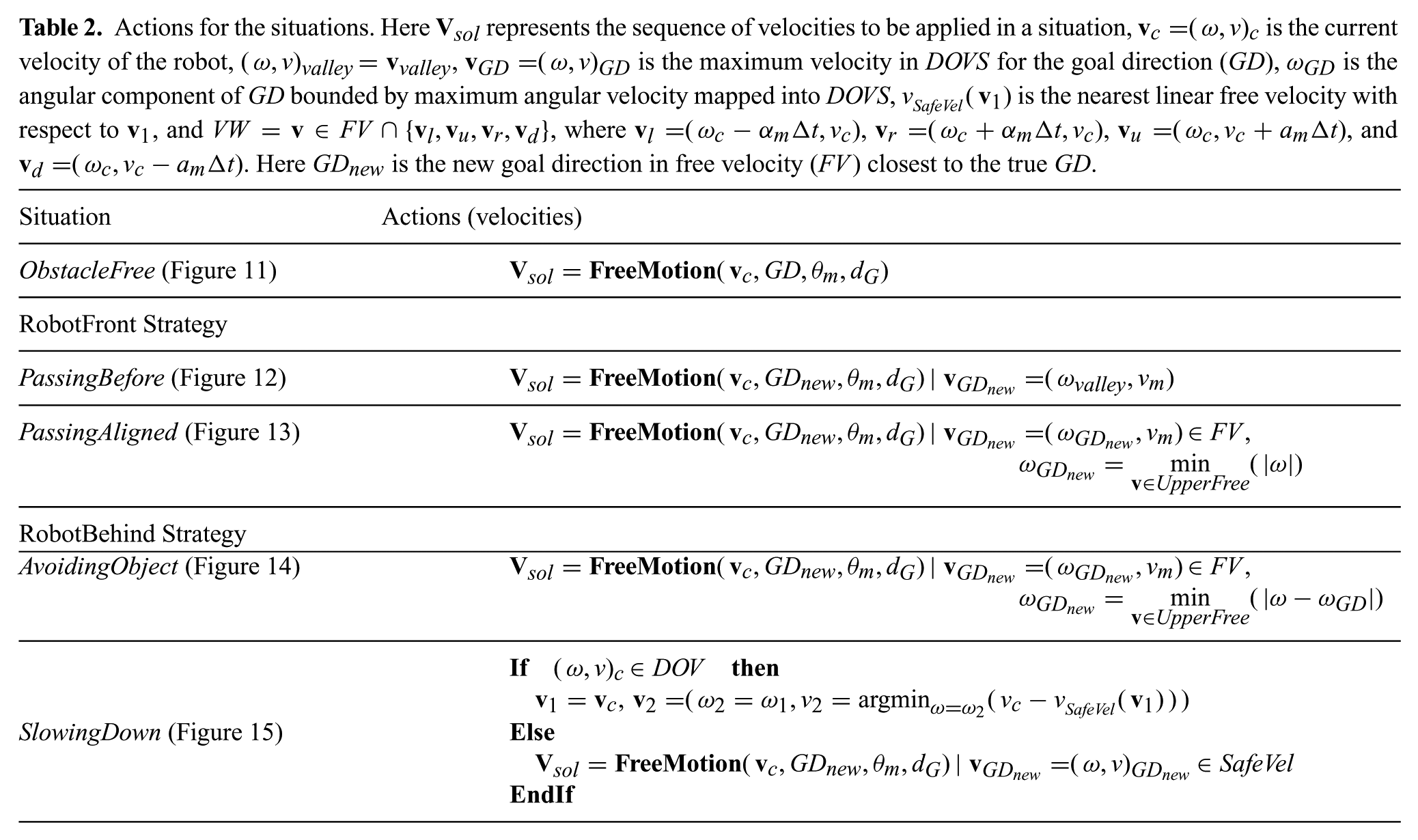
The planner reasons in the DOVS space described in Section 5, which maps the environment dynamism of obstacles. In a scenario with obstacles, the trajectories introduced before do not lead to time-optimal trajectories because they may result in collisions. However, it is possible to find near-time-optimal and safe trajectories computed in the free velocity space $F V$ , easily identifiable in DOVS. Thus, the methodology presented in Section 6.2 is applicable in this space, avoiding obstacles whilst preserving low time-to-goal motions and safety.

The strategies are associated to situations detected. Figure 10 shows the situation tree, where the leaves correspond to all the situations that can be identified. Each of the situations has an associated action; the sequence of actions applied to reach the goal constitutes a strategy, which implements the general decision making process described in Section 6. The robocentric planner executes cyclically, performing the strategies and so adapting to the changing environment in real-time. The planner establishes a long-term plan within the horizon defined by the field of view of the sensors and not only for the next sampling period. In this sense, this local planner is not purely reactive. It computes a safe trajectory for that space horizon. The plan is re-computed for each sampling period, so only the immediate action of the strategy required by the current situation is applied at each sampling time.

Fig. 10.

Situation tree. Leaves represent all the situations that can be identified, each of which has an associated navigation strategy.

Table 2 shows the actions associated with each situation. Roughly speaking, the method consists in applying a sequence of maximum angular and linear accelerations to reach the maximum linear velocity in the free velocity space ( $F V$ ), following the command computation developed in Section 6.2. Before doing it, if the goal direction mapped in the velocity space, $G D$ , is inside a dynamic obstacle DOV, a close new goal $G D_{n e w}$ is mapped in $F V$ in each situation. This way the near-time-optimal command sequence is applied to reach that goal, avoiding the moving obstacle until $G D$ is in $F V$ again.

Table 2.

Actions for the situations. Here $V_{s o l}$ represents the sequence of velocities to be applied in a situation, $v_{c} = (ω, v)_{c}$ is the current velocity of the robot, ${(ω, v)}_{v a l l e y} = v_{v a l l e y}$ , $v_{G D} = (ω, v)_{G D}$ is the maximum velocity in DOVS for the goal direction ( $G D$ ), $ω_{G D}$ is the angular component of $G D$ bounded by maximum angular velocity mapped into DOVS, $v_{S a f e V e l} (v_{1})$ is the nearest linear free velocity with respect to $v_{1}$ , and $V W = v \in F V \cap {v_{l}, v_{u}, v_{r}, v_{d}}$ , where $v_{l} = (ω_{c} - α_{m} Δ t, v_{c})$ , $v_{r} = (ω_{c} + α_{m} Δ t, v_{c})$ , $v_{u} = (ω_{c}, v_{c} + a_{m} Δ t)$ , and $v_{d} = (ω_{c}, v_{c} - a_{m} Δ t)$ . Here $G D_{n e w}$ is the new goal direction in free velocity ( $F V$ ) closest to the true $G D$ .

Situation	Actions (velocities)
$O b s t a c l e F r e e$ (Figure 11)	$V_{s o l} = FreeMotion (v_{c}, G D, θ_{m}, d_{G})$
RobotFront Strategy
$P a s s i n g B e f o r e$ (Figure 12)	$V_{s o l} = FreeMotion (v_{c}, G D_{n e w}, θ_{m}, d_{G}) \| v_{G D_{n e w}} = (ω_{v a l l e y}, v_{m})$
$P a s s i n g A l i g n e d$ (Figure 13)	$V_{s o l} = FreeMotion (v_{c}, G D_{n e w}, θ_{m}, d_{G}) \| v_{G D_{n e w}} = (ω_{G D_{n e w}}, v_{m}) \in F V,$
	$ω_{G D_{n e w}} = \min_{v \in U p p e r F r e e} (\| ω \|)$
RobotBehind Strategy
$A v o i d i n g O b j e c t$ (Figure 14)	$V_{s o l} = FreeMotion (v_{c}, G D_{n e w}, θ_{m}, d_{G}) \| v_{G D_{n e w}} = (ω_{G D_{n e w}}, v_{m}) \in F V,$
	$ω_{G D_{n e w}} = \min_{v \in U p p e r F r e e} (\| ω - ω_{G D} \|)$
	$If {(ω, v)}_{c} \in D O V then$
	$v_{1} = v_{c}, v_{2} = (ω_{2} = ω_{1}, v_{2} = {argmin}_{ω = ω_{2}} (v_{c} - v_{S a f e V e l} (v_{1})))$
$S l o w i n g D o w n$ (Figure 15)	$Else$
	$V_{s o l} = FreeMotion (v_{c}, G D_{n e w}, θ_{m}, d_{G}) \| v_{G D_{n e w}} = (ω, v)_{G D_{n e w}} \in S a f e V e l$
	$EndIf$

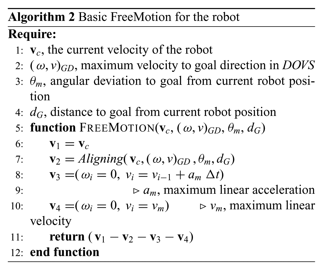
Algorithm 2 represents the basic motion to be applied in all situations, as shown in Table 2. The only difference between situations is the election of a new $G D_{n e w}$ in the free-velocity space $F V$ . Figures 11 –15 describe situations ObstacleFree, PassingBefore, PassingAligned, AvoidingObject, and SlowingDown, its associated actions and the strategies derived from them. The AvoidingCollision situation is a consequence of the robot having entered the collision band of an obstacle and then having to execute a velocity in free space to avoid collision. The CertainCollision situation appears when the robot falls into an unavoidable collision situation, due either to an unexpected obstacle appearing on the scene, or because no free velocity is available (a blocking situation, e.g. objects surrounding the robot).

Algorithm 2 Basic FreeMotion for the robot
Require:
1: $v_{c}$ , the current velocity of the robot
2: ${(ω, v)}_{G D}$ , maximum velocity to goal direction in $D O V S$
3: $θ_{m}$ , angular deviation to goal from current robot position
4: $d_{G}$ , distance to goal from current robot position
5: function FreeMotion( $v_{c}$ , ${(ω, v)}_{G D}$ , $θ_{m}$ , $d_{G}$ )
6: $v_{1} = v_{c}$
7: $v_{2} = A l i g n i n g (v_{c}, (ω, v)_{G D}, θ_{m}, d_{G})$
8: $v_{3} = (ω_{i} = 0, v_{i} = v_{i - 1} + a_{m} Δ t)$
9: ▷ $a_{m}$ , maximum linear acceleration
10: $v_{4} = (ω_{i} = 0, v_{i} = v_{m})$ ▷ $v_{m}$ , maximum linear Velocity
11: return $(v_{1} - v_{2} - v_{3} - v_{4})$
12: end function

Fig. 11.

Evolution of the ObstacleFree situation. Algorithm 2 implements the motion for this situation. (a) Part of the trajectory followed by the robot. (b)–(d) Velocity space of the robot and the applied actions in three representative locations of the trajectory. The vertical red line represents the steering direction $S D$ and the black line the goal direction $G D$ , to be reached for alignment to the goal. In $L o c_{1}$ a maximum angular acceleration ( $v_{1}$ – $v_{2}$ ) is applied to reach $S D$ every sampling period (the angular deviation of the robot is high). In $L o c_{2}$ a maximum angular deceleration ( $v_{2}$ – $v_{3}$ ) is applied to reach $G D$ (the angular deviation has decreased). In $L o c_{3}$ the robot applies commands at maximum linear acceleration ( $v_{3}$ – $v_{4}$ ), while in $L o c_{4}$ and $L o c_{5}$ , a straight line at maximum linear velocity $v_{4}$ is achieved.

Fig. 12.

Evolution of the PassingBefore situation. (a) Trajectory of the robot. (b)–(e) DOVS at four relevant instants during the trajectory. In this situation the robot can cross the collision band to pass before the object. There is a set of free velocities in the $U p p e r F r e e$ zone which can be reached inside the bounds of the $D O V$ ( $V_{u p}$ ), identified as a valley. The depth of the valley ( $v_{v a l l e y}$ in Table 1) provides certain knowledge about the level of safety for the robot to perform the strategy. The deeper the valley, the greater its width, and the safer it is to traverse the $D O V$ to reach the free velocities in $V_{u p}$ . A new $G D_{n e w}$ is computed close to the initial $G D$ in $V_{u p}$ , such that it contains velocity $v_{v a l l e y}$ . A sequence of clothoid ( $v_{1}$ – $v_{2}$ ) at maximum angular deceleration (b), anti-clothoid ( $v_{2}$ – $v_{3}$ ) at maximum linear acceleration (c), (d), and straight line at maximum linear velocity is applied (e).

Fig. 13.

Evolution in the PassingAligned situation. (a) Trajectory performed by the robot. (b)–(d) DOVS for different motions of the robot. The set of velocities in $U p p e r F r e e$ leads the robot to move in the same direction as the object. In this case, the robot lies inside the $D O V$ and $G D$ is not free. Here $G D_{n e w}$ is defined to escape from dangerous velocities, applying an angular acceleration motion (clothoid $v_{1}$ – $v_{2}$ ). Then, maximum linear acceleration ( $v_{2}$ – $v_{3}$ ) is applied to move in the same direction as the obstacle ( $L o c_{3}$ ). If the robot moves faster than the object, a valley appears inside $D O V$ , which allows the robot to change the strategy to a PassingBefore situation. Finally, AvoidingCollision ( $L o c_{4}$ ) and ObstacleFree ( $L o c_{5}$ ) situations are identified when the robot lies inside the collision band and when it exits it, respectively.

Fig. 14.

Evolution of the AvoidingObject situation. (a) Partial trajectory of the robot. (b)–(d) DOVS representation at different instants. In this situation, the $D O V$ of a moving object occupies the middle zone of DOVS, leaving two zones of velocities in $U p p e r F r e e$ that belong to $V_{s i d e}$ (b). A new $G D_{n e w}$ close to the current $G D$ is selected in $V_{s i d e}$ , to then apply the sequence of motions computed by Algorithm 2. The robot manoeuvres to pass behind the object.

Fig. 15.

Evolution in the SlowingDown situation. (a) Trajectory of the robot. (b)–(e) DOVS information at different locations of the robot. There are no $U p p e r F r e e$ velocities in DOVS (see Figure 15(a) and (b)). In this case, the velocity of the robot is inside the $D O V$ of the object, and the robot has to slow down to avoid a collision. A sequence of anti-clothoid trajectories (deceleration) is applied to escape from the dangerous velocities ( $v_{1}$ – $v_{2}$ ). Then, a sequence of clothoid trajectories ( $v_{2}$ – $v_{3}$ – $v_{4}$ ) is computed to maintain the robot at a low safe velocity in the $S a f e V e l$ zone until the object passes (c), following a new $G D_{n e w}$ computed in $S a f e V e l$ . The set $S a f e V e l$ defines the velocities which will be freed first, given the motion of the object. Finally an ObstacleFree situation appears (e), and the corresponding strategy is applied.

7. Experimental evaluation and metrics

7.1. Simulation results

In this section we evaluate the proposed technique qualitatively and quantitatively. Simulations where the robot traverses the scenario to reach different goals are shown in Extension 1.¹

In these scenarios only moving objects appear around the robot. We have considered obstacle occupancies of $4 %$ and $7 %$ (Figure 16), given that the $4 %$ value is a commonly found scenario in the literature (Bareiss and Van den Berg, 2015; Martinez-Gomez and Fraichard, 2009). Although these occupancies are seemingly not very dense when compared to static benchmark scenarios, the large impact of moving obstacles in the effective space for safe planning (see Figure 16) makes them suitably challenging. This effective space has been computed as the mean of the forbidden velocity areas in DOVS, a way to quantify the limited robot manoeuvrability. See Table 3.

Fig. 16.

Scenarios with different densities of occupancy: (a) $7 %$ of static density corresponds to $46 %$ of occupancy in terms of safe velocity space available to be chosen in the linear scenario; (b) $4 %$ of static occupancy represents about $35 %$ of forbidden velocities in the non-linear scenario with obstacles moving in circular trajectories.

Table 3.

Mean of forbidden velocity area in DOVS during simulations for different obstacle velocity ranges. The values of $4 %$ and $7 %$ for obstacle occupancy were measured as the area of the workspace occupied by the obstacles at a given instant (as if the obstacles were static). However, if we measure the occupancy in terms of forbidden velocities in DOVS as the area of each DOV, these values increase considerably.

	$V_{1}$	$V_{2}$	$V_{3}$
	$v = 0.2$	$v = 0.5$	$v = 0.6 . . 0.9$
Linear	$ω = 0$
$4 %$ occupancy	$34.85 %$	$40.12 %$	$42.67 %$
$7 %$ occupancy	$46.08 %$	$53.98 %$	$58.19 %$
Non-linear	$ω =$	$ω =$	$ω =$
	$- 0.15 . . 0.15$	$- 0.38 . . 0.38$	$- 0.45 . . 0.45$
$4 %$ occupancy	$34.97 %$	$39.17 %$	$40.06 %$

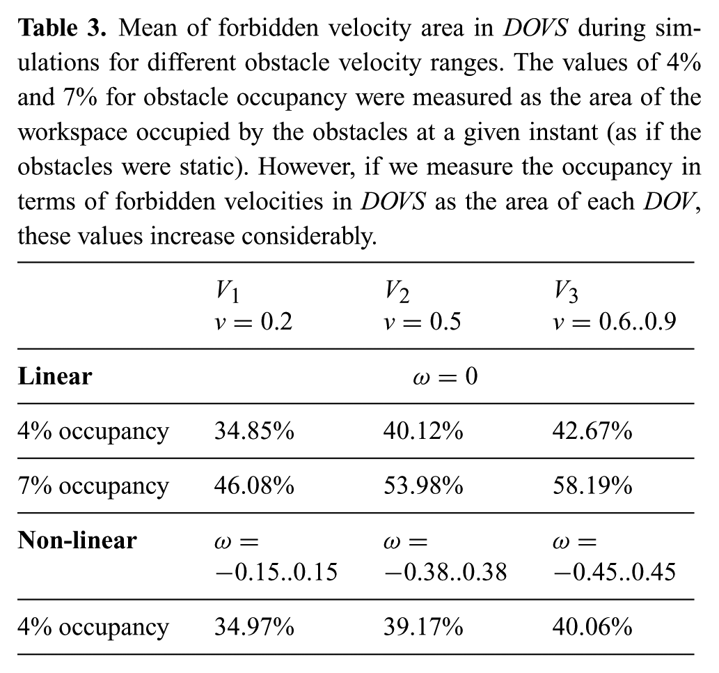
We have tested navigation for three different types of scenario during simulation: linear, non-linear, both for moving obstacles, and complete, having static and moving obstacles. A total of $40$ different scenarios are simulated in linear and non-linear sets. In each scenario the robot has to reach four different goals. In total, we have run $1440$ simulations, $160$ for $each %$ of obstacle occupancy ( $4 %$ and $7 %$ for linear, $4 %$ for non-linear), for the three sets of velocities $V_{1}, V_{2}, V_{3}$ described in Table 3, and for a maximum linear robot velocity of 1.5 m $s^{- 1}$ .

We have evaluated the technique in scenarios where the density of obstacles remains the same, so static bounds were established to define the workspace and simulate the movement of the obstacles cyclically, once the random movement has been generated. Table 4 reflects the collisions produced during simulation, as explained later. Column Bounded ( $V_{1}$ ) indicates the percentage of collisions in scenarios with static bounds. A first observation is that the number of collisions is greater than in open scenarios, represented in the other three columns, due to the robot being trapped when it is close to them. Therefore, to focus on the evaluation of the robot navigating among moving obstacles, we have discarded the static bounds to evaluate the performance based on metrics. Another reason for collisions is because new obstacles appear from outside the limits of the scenario, so the robot might not have the reaction capability from kinodynamic constraints to avoid collision. In addition, we have evaluated the method when conditions about obstacle motion is uncertain, scenario NL-Approx. Thus, we have performed simulations in scenarios with obstacles moving with non-linear trajectories and approximating the DOVS model with the linear approach. The collisions greatly increase, as can be seen in Table 4. Therefore, the method benefits from the greater lookahead if there is a proper estimation of the obstacle motion. Whenever the motion changes, the calculations should be recomputed and, in this case, our method behaves like a reactive one.

Table 4.

Percentage of collisions during simulations. Note that in the highest-occupancy situations and with the scenario bounds acting as static obstacles, many trapping situations can appear so some inevitable collisions occur.

	Bounded	$V_{1}$	$V_{2}$	$V_{3}$
	( $V_{1}$ )
Linear
$4 %$ occupancy	$5 %$	$0 %$	$2.5 %$	$3.75 %$
$7 %$ occupancy	$32.5 %$	$5 %$	$10 %$	$16.875 %$
Non-linear
$4 %$ occupancy	$10.6 %$	$3.75 %$	$15 %$	$11.875 %$
NL-Approx
$4 %$ occupancy		$10.62 %$	$34.37 %$	$46.25 %$

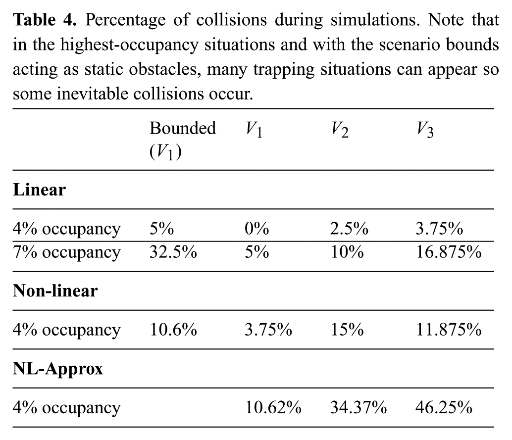
Figure 17 illustrates several iterations of a simulation of the linear scenarios. The robot manoeuvres around the obstacles while maintaining safety, selecting high velocities in the free velocity sub-space $F V$ .

Fig. 17.

Simulation in a linear scenario for $4 %$ obstacle occupancy and velocities in $V_{1}$ . In fact, this percentage increases in a dynamic scenario, as a result of the reduction on the available workspace and velocity space. The workspace (left) and DOVS (right) are represented at different instants. The planner searches for free velocity sub-spaces so that the robot (red) can maintain high linear velocities (rhomboid window) during navigation.

Figures 18 and 19 show several metrics evaluated during navigation for the overall simulations in linear scenarios, for each of the occupancy densities considered and for each set of velocities. As expected, in a scenario where fewer obstacles appear, the robot can move at higher velocities (Figures 18(a) and 19(a)). Safety is evaluated from the distance measured between the robot and each of the obstacles (Figures 18(b) and 19(b)). Figures 18(c) and 19(c) illustrate the time-to-goal with respect to the optimal value for each goal, computed for free space. Longer trajectories are produced when there are more obstacles in the environment. Figures 18(d) and 19(d) describe the strategies selected during navigation. AvoidingObject and AvoidingCollision are the most frequently applied strategies. PassingBefore strategy occurs more frequently than SlowingDown, which means that the robot tries to search for free spaces to pass before objects at high velocity, rather than slowing down to give way to objects. It can be seen that for $7 %$ occupancy ObstacleFree and PassingBefore appear less frequently than for $4 %$ occupancy, as was predictable.

Fig. 18.

Metrics for $4 %$ occupancy scenarios with obstacles moving linearly. Percentile, mean, and median for: (a) linear velocity, (b) distance to obstacles, (c) time with respect to optimal for free space, and (d) histogram of the situations.

Fig. 19.

Metrics for $7 %$ occupancy scenarios, with obstacles moving linearly.

Regarding simulations for non-linear scenarios, Figure 20 plots the same metrics as for the linear scenarios. Similar results are obtained, so the technique adapts well to different kinds of obstacle trajectories.

Fig. 20.

Metrics for simulations for $4 %$ occupancy of non-linear obstacles.

Moreover, the technique developed is conservative in the sense that any velocity in free velocity space $F V$ is safe, but the velocities inside a DOV do not always or instantly lead to an unavoidable collision; they can be selected but only during a certain time without collision. This improvement is the subject of future work.

Finally, in the complete scenario shown in Figure 21 there are static and moving obstacles (following linear and non-linear trajectories) to illustrate a general situation in which a robot has to move from one room to another, navigating among several objects and four subgoals (waypoints). Figure 22 represents the metrics. In this scenario, where many static objects are present and appear in DOVS, the ObstacleFree situation is not encountered, so there are not many velocities free to manoeuver.

Fig. 21.

Complete scenario with static (black), linear, and non-linear obstacles describing their trajectory (blue), and the trajectory performed by the robot (red) to achieve the different goals.

Fig. 22.

Metrics for simulation of the complete scenario. Most of the time the robot moves at maximum velocity, slowing down when it becomes considerably disorientated from the goal (bigger changes observed for angular velocity). Strategy PassingBefore is applied many times, that is the robot moves many times at high velocities to pass before the obstacles, and no CertainCollision situation appears.

7.2. Comparison with a one-step approach

We show here through simulation how our lookahead planner obtains a better behavior and lower time-to-goal than a method that considers only the next-period candidate velocities. This local planning approach is denominated one-step approach, and it is the decision process used in Gal et al. (2009) and Shiller et al. (2010) to develop a near-time-optimal motion planner. The basic idea is that the planner chooses collision-free velocities from the velocity window ( $V W$ ) that generate a time-optimal trajectory to the goal, evaluated in absence of obstacles. In our case, for a non-holonomic robot, the near-time-optimal motions used are those introduced in Section 6.2. The planner proposed in this work computes collision-free commands from the velocity window based on the future evolution of the obstacles, lookahead information previously considered to plan a safe trajectory to the goal, by choosing a Goal Direction ( $G D$ ) outside DOV.

The evaluation carried out is performed in randomly generated scenarios, where the robot has to reach four different goals, during a set of $10$ simulations. The range of velocities considered for the obstacles are: $0.2$ , $0.5$ , $0.8$ , and $1.2$ . Figure 23 shows the mean values of the time-to-goal for each of the methods. It can be seen that for low obstacle velocities, our approach gets better results, whereas similar values are obtained with higher velocities. This is because the obstacles spend more time occupying the workspace: the one-step approach remains in the time-optimal trajectory for the current $V W$ , whereas our approach favors the selection of commands towards bigger areas of free space. Therefore, both approaches obtain near-time-optimal trajectories, but ours can achieve lower times to the goal.

Fig. 23.

Comparison of the mean of the time-to-goal for our lookahead planner and the one-step local method, for the velocity range considered.

Figure 24(a) and (b) plot a scenario for one of the simulations designed, where the robot behavior using both methods to move around the obstacles is also shown. As can be seen, our method makes the robot to pass between both obstacles, whereas the one-step approach computes a longer trajectory due to the implicit reactivity of the local planning. As a consequence, the time-to-goal and the trajectory length are reduced (Figure 24(c) and (d)).

Fig. 24.

Trajectories followed by the robot reasoning within DOVS visibility (a) and one-step visibility (b). Profiles of linear (c) and angular (d) velocities during navigation. Looking further ahead at a single instant (DOVS) provides shorter and lower time-to-goal trajectories than using the theoretical time-optimal control to the goal at every sampling time (one-step approach).

Figure 25 describes several steps of the simulation for both methods. DOVS lookahead plans long-term manoeuvres in the velocity free space, which permits to find safe commands when re-planning every sampling time to move between both obstacles, unlike one-step planner that only re-plans locally to follow a theoretical time-optimal trajectory towards the goal in the free space.

Fig. 25.

(a)–(e) One-step local planner: the velocity which would drive the robot to the goal applying time-optimal commands from the current position–velocity in free space (mapped $G D$ ) is selected. In (d) the velocity obstacle prevents the robot from choosing a velocity to manoeuvre towards the goal, until the moving object passes and $G D$ becomes free to be followed (e). (f)–(j) DOVS lookahead planner: it plans safe velocities out of the velocity obstacle for the sensor visibility horizon, driving the robot to the new mapped goal $G D_{n e w}$ (f)–(h) instead of $G D$ , leading the robot to slow down and manoeuvre to finally cross between both obstacles through the velocity valley (i), (j).

7.3. Real-world experiments

The first scenario corresponds to the kind of scenarios shown in the simulations with obstacles moving randomly in all directions. The second is a more structured scenario, an overtaking manoeuvre. Extension 2 contains a video of the experiments.

7.3.1. Experimental setup

The navigation strategies have been tested on three Pioneer robots. These are differential-drive robots equipped with a 2D laser rangefinder Sick LMS-200 and on-board Intel Centrino duo at $1.6$ GHz. The computation time of the navigation strategies was around 200 ms, the time for which a new laser measuring is available. The field of view of the laser rangefinder sensor was $180^{\circ}$ , ${0.5}^{\circ}$ of angular resolution and a maximum range of 8 m. The maximum translational velocity was set to $0.3$ m $s^{- 1}$ and the rotational velocity to $0.4$ rad $s^{- 1}$ , fitting the velocity window used. The method developed by Montesano et al. (2008) is used for mapping static and moving obstacles from rangefinder sensors, and an extended Kalman filter (EKF)-based technique is applied to track the moving objects, in which the state vector included the location and the velocities of the tracked objects.

The work presented in Prassler et al. (2001) developed a navigation system on a wheelchair equipped with sensors. The authors represent the space occupied at instant $t$ with a time stamp map, and compare the corresponding information in the previous step to determine moving and static obstacles by using a nearest-neighbor criterion. The VO approach is used to compute safe velocities, selecting the highest feasible velocity in the direction of the goal or a manoeuvre-avoidance velocity with a specific heading. As a result, wall-following and obstacle-avoidance behaviors are observed in simulation and real-world crowded environments.

7.3.2. Experiment 1

Figure 26(a) depicts the hall-like scenario, with robot and object trajectories, not previously known. Figure 26(b)–(d) shows the velocity profiles and the strategies. ObstacleFree, AvoidingObject, and PassingBefore are the most frequent situations, allowing to maintain the maximum linear velocity. Figure 27 illustrates several steps of the experiment.

Fig. 26.

Hall scenario: (a) trajectory of the robot (green) and environment perceived in experiment 1, with static and moving objects; (b) linear velocity profile; (c) angular velocity profile; (d) situations.

Fig. 27.

Experiment 1 in the hall ( $r a n d o m$ ) scenario. The robot can pass between $O b j 1$ and $O b j 2$ (a), (b) at maximum velocity (c), and avoids $O b j 3$ (d), (e) towards the side closest to the goal (f).

7.3.3. Experiment 2

Figures 28(a) and 29 show an overtaking manoeuvre in a narrow corridor. Before overtaking obstacle 1, the robot slows down until obstacle 2 passes. When the manoeuvre is initiated, the maximum velocity is maintained until the end (Figure 28(b)). ObstacleFree, AvoidingObject, and SlowingDown are the situations that occur the most. The latter makes the robot reduce the velocity before starting the overtaking manoeuvre.

Fig. 28.

Overtaking scenario: (a) trajectory of the robot (green) and environment perceived in experiment 2, (b) linear velocity profile, (c) angular velocity profile, and (d) situations.

Fig. 29.

Experiment 2 in the Overtaking scenario. The robot has to slow down before overtaking obstacle $O b j 1$ . Red velocity obstacles (c) are the walls on both sides of the corridor and obstacle $O b j 1$ , which is detected as static given that both the robot and $O b j 1$ are navigating with a similar velocity.

8. Conclusions

A robocentric technique for planning and navigation in dynamic environments has been developed. The DOVS model defined for mapping the dynamics of the environment allows the planning of safe motions within a space horizon, for instance the range of visibility of the onboard sensors. Several situations depending on the decision variables are identified applying specific actions associated to them, which implement the $R o b o t F r o n t$ or the $R o b o t B e h i n d$ strategies. The complexity of the method does not increase either by trajectories that are more complex than linear obstacle trajectories, or as a result of the space–time horizon for planning, unlike other techniques described in the literature. It has been shown that the long-term strategies selected every sampling time within the space horizon visibility improve the time to goal with respect to other techniques that are purely reactive. The method has been evaluated in simulation and in real-world experiments. In a dynamic scenario, the navigation difficulty can be measured from the velocity space area occupied by the obstacles, which somehow reflects the actual capability of the robot to manoeuvre. Sometimes collisions are unavoidable, mainly in cases where the robot is trapped near static obstacles or when obstacles appear in the scenario, due to robot’s kinodynamic constraints.

From the lessons learned, some improvements are being considered for future work. Using directly the DOV obstacles without merging them would make the processing more complex but enlarge the set of free and safe velocities to be selected to manoeuvre. Blocking situations appearing in closed scenarios or with many static obstacles could be reduced achieving a different treatment for those static obstacles, by prioritizing free and safe velocities that move the robot away from them. In the context of a multi-agent scenario in which several mobile robots can make decisions, a future work will be focused on the extension of the model and development of planning techniques to share the decision-making process among several robots to obtain mutually optimized plans.

Footnotes

Appendix A: Index to multimedia extensions

Archives of IJRR multimedia extensions published prior to 2014 can be found at http://www.ijrr.org, after 2014 all videos are available on the IJRR YouTube channel at http://www.youtube.com/user/ijrrmultimedia

SAGE-Journals-Accessible-Video-Player 10.1177/0278364918775520.M1 sj-vid-1-ijr-10.11770278364918775520 Extension 1

Simulations to show the navigation performance of the robot in several scenarios and conditions.

SAGE-Journals-Accessible-Video-Player 10.1177/0278364918775520.M2 sj-vid-2-ijr-10.11770278364918775520 Extension 2

Real experiments in two scenarios: a hall-like scenario, and an overtaking-like manoeuvre.

Appendix B: Computation of the robotcollision velocities

Appendix C: Computation of time to goal from the current robot location

Trajectories are composed of combinations of straight lines, circular, clothoid, and anti-clothoid curves. The time-to-goal functions ( $t_{G}$ ) are computed as the sum of several terms, the switching times: time for angular acceleration ( $t_{α}$ ), time for linear acceleration at constant angular non-zero velocity ( $t_{a w}$ ), time at constant angular velocity ( $t_{w}$ ), time for angular deceleration until alignment with the goal ( $t_{- α}$ ), time for linear acceleration once the robot is aligned ( $t_{a}$ ), and time at maximum linear velocity towards the goal ( $t_{v}$ ). The total time to goal in both cases is

\begin{array}{l} t_{G w} = t_{α} + t_{w} + t_{- α} + t_{a} + t_{v} (clothoid) \\ t_{G v} = t_{a w} + t_{- α} + t_{a} + t_{v} (anti - clothoid) \end{array}

The switching time for starting angular deceleration is computed when $θ_{a} = ω_{c}^{2} / 2 * α_{m}$ is reached, being $ω = 0$ when the robot is aligned to the goal ( $x_{G}, y_{G}$ ). The switching times are computed as follows.

(a) Time for angular acceleration ( $t_{α}$ )/deceleration ( $t_{- α}$ )

\begin{array}{l} t_{α} = (w_{α} - w_{c}) / α_{m} \\ ω_{α} = \min (ω_{t o p_{w}}, ω_{m}); ω_{t o p_{w}} = w_{c} + α_{m} * t_{t o p_{w}} \\ t_{- α} ≃ w_{c} / α_{m}; ω_{t_{- α}} = w_{c} - α_{m} * t_{- α} ≃ 0 \end{array}

Velocity $ω_{α}$ will be the angular velocity reached ( $ω_{t o p_{w}}$ ) when the value $θ_{a} = ω_{c}^{2} / 2 * α_{m}$ with respect to the goal direction is measured or $ω_{m}$ is reached, whilst $v_{c}$ is kept. Then an angular deceleration starts until aligning the goal. The coordinates at the end this stage are ( $β = {α, - α}$ )

\begin{array}{l} x_{β} = v_{c} * \int_{t_{0}}^{t_{β}} \cos (θ (t)) d t \\ y_{β} = v_{c} * \int_{t_{0}}^{t_{β}} \sin (θ (t)) d t \\ θ_{β} = w_{c} * t_{β} + (α_{m} * t_{β}^{2}) / 2 \end{array}

These are non integrable equations, so they are solved numerically.

(b) Time at constant angular velocity ( $t_{w}$ ). Time until the orientation reaches $θ_{a}$ from the initial $θ_{c}$ :

t_{w} = (θ_{c} - θ_{a}) / ω_{c}

Both the angular and linear velocities $(v_{c}, ω_{c})$ are kept. The coordinates at the end of this stage are

\begin{array}{l} x_{ω} = (v_{c} / ω_{c}) * \sin (θ_{c} - θ_{a}) \\ y_{ω} = (v_{c} / ω_{c}) * (1 - \cos (θ_{c} - θ_{a})) \\ θ_{ω} = θ_{c} - θ_{a} \end{array}

(c) Time at maximum linear acceleration and constant angular velocity ( $t_{a w}$ ):

\begin{array}{l} t_{a w} = (v_{a w} - v_{c}) / a_{m}; v_{a w} = \min (v_{t o p_{v}}, v_{m}) \\ v_{t o p_{v}} = v_{c} + a_{m} * t_{t o p_{v}} \end{array}

This stage finishes when the angular position with respect to the goal direction ( $θ_{a}$ ) is reached. The coordinates reached at the end of this stage are

\begin{array}{l} x_{a w} = \int_{t_{0}}^{t_{a w}} v (t) * \cos (θ (t)) d t \\ y_{a w} = \int_{t_{0}}^{t_{a w}} v (t) * \sin (θ (t)) d t \\ θ_{a w} = w_{c} * t_{a w} \end{array}

(d) Time at maximum linear acceleration ( $t_{a}$ ):

t_{a} = (v_{m} - v_{c}) / a_{m}; v_{a} = v_{c} + a_{m} * t_{a}

The stage starts when the robot is aligned ( $ω = 0, θ_{a} = 0$ ), and accelerates up to the maximum linear velocity. The coordinates reached are

\begin{array}{l} x_{a} = (v_{c} + (a_{m} * t_{a}) / 2) * \cos (θ_{g}) * t_{a} \\ y_{a} = (v_{c} + (a_{m} * t_{a}) / 2) * \sin (θ_{g}) * t_{a} \end{array}

(e) Time at maximum linear velocity ( $t_{v}$ ). At the start of this stage, the current location of the robot is given by

x_{c} = \sum_{i} x_{i}, y_{c} = \sum_{i} y_{i}, i = α, w, a_{w}, - α, a

With $d_{G}$ begin the distance to the goal from $(x_{c}, y_{c})$ , the time to goal and velocities are

t_{v} = d_{G} / v_{v}, v_{v} = v_{m}, w_{v} = 0

Funding

The author(s) disclosed receipt of the following financial support for the research, authorship, and/or publication of this article: This work was partially supported by project DPI2016-76676-R and project DGA T04-FSE.

Notes

References

Althoff

Wollherr

Buss

(2010) Probabilistic collision state checker for crowded environments. In: 2010 IEEE International Conference on Robotics and Automation (ICRA), pp. 1492–1498.

Althoff

Kuffner

Wollherr

Buss

(2012) Safety assessment of robot trajectories for navigation in uncertain and dynamic environments. Autonomous Robots 32(3): 285–302.

Arkin

(1998) An Behavior-based Robotics. 1st edition. Cambridge, MA: MIT Press.

Balkcom

Mason

(2002) Time optimal trajectories for bounded velocity differential drive vehicles. The International Journal of Robotics Research 21(3): 199–217.

Bareiss

Van den Berg

(2013) Reciprocal collision avoidance for robots with linear dynamics using LQR-obstacles. In: 2013 IEEE International Conference on Robotics and Automation (ICRA), pp. 3847–3853.

Bareiss

Van den Berg

(2015) Generalized reciprocal collision avoidance. The International Journal of Robotics Research 34(12): 1501–1514.

Bautin

Martinez-Gomez

Fraichard

(2010) Inevitable collision states: A probabilistic perspective. In: 2010 IEEE International Conference on Robotics and Automation (ICRA), pp. 4022–4027.

Bekris

Kavraki

(2007) Greedy but safe replanning under kinodynamic constraints. In: Proceedings 2007 IEEE International Conference on Robotics and Automation, pp. 704–710.

Bekris

Tsianos

Kavraki

(2009) Safe and distributed kinodynamic replanning for vehicular networks. Mobile Networks and Applications 14(3): 292–308.

10.

Bouraine

Fraichard

Azouaoui

Salhi

(2014) Passively safe partial motion planning for mobile robots with limited field-of-views in unknown dynamic environments. In: 2014 IEEE International Conference on Robotics and Automation (ICRA), pp. 3576–3582.

11.

Bouraine

Fraichard

Salhi

(2012) Provably safe navigation for mobile robots with limited field-of-views in dynamic environments. Autonomous Robots 32(3): 267–283.

12.

Brock

Khatib

(2000) Real-time re-planning in high-dimensional configuration spaces using sets of homotopic paths. In: Proceedings IEEE International Conference on Robotics and Automation, 2000 (ICRA ’00), vol. 1, pp. 550–555.

13.

Chan

Kuffner

Zucker

(2008) Improved motion planning speed and safety using regions of inevitable collision. In: 17th CISM-IFToMM Symposium on Robot Design, Dynamics, and Control (RoManSy’08).

14.

Fiorini

(1995) Robot Motion Planning Among Moving Obstacles. PhD Thesis (UMI Order No. GAX95-19816), University of California, Los Angeles, CA, USA.

15.

Fiorini

Shiller

(1998) Motion planning in dynamic environments using velocity obstacles. The International Journal of Robotics Research 17(7): 760–772.

16.

Fox

Burgard

Thrun

(1997) The dynamic window approach to collision avoidance. IEEE Robotics Automation Magazine 4(1): 23–33.

17.

Fraichard

(1998) Trajectory Planning in Dynamic Workspace: a ‘State-Time Space’ Approach. Technical Report RR-3545, INRIA.

18.

Fraichard

(2007) A short paper about motion safety. In: Proceedings 2007 IEEE International Conference on Robotics and Automation, pp. 1140–1145.

19.

Fraichard

Asama

(2003) Inevitable collision states. a step towards safer robots? In: Proceedings 2003 IEEE/RSJ International Conference on Intelligent Robots and Systems, 2003 (IROS 2003), vol. 1, pp. 388–393.

20.

Frazzoli

Dahleh

Feron

(2001) Real-time motion planning for agile autonomous vehicles. In: Proceedings of the 2001 American Control Conference, vol. 1, pp. 43–49.

21.

Gal

Shiller

Rimon

(2009) Efficient and safe on-line motion planning in dynamic environments. In: Proceedings IEEE International Conference on Robotics and Automation, Kobe, Japan, pp. 188–93.

22.

Hsu

Kindel

Latombe

Rock

(2002) Randomized kinodynamic motion planning with moving obstacles. The International Journal of Robotics Research 21(3): 233–255.

23.

Kalisiak

van de Panne

(2007) Faster motion planning using learned local viability models. In: Proceedings 2007 IEEE International Conference on Robotics and Automation, pp. 2700–2705.

24.

Kim

(2016) Study on optimal velocity selection using velocity obstacle (OVVO) in dynamic and crowded environment. Autonomous Robots 40(8): 1459–1470.

25.

Large

Laugier

Shiller

(2005) Navigation among moving obstacles using the NLVO: Principles and applications to intelligent vehicles. Autonomous Robots 19(2): 159–171.

26.

Large

Sekhavat

Shiller

Laugier

(2002) Using non-linear velocity obstacles to plan motions in dynamic environments. In: IEEE International Conference on Control, Automation, Robotics and Vision (ICARV02), pp. 734–739.

27.

LaValle

Kuffner

(2001) Randomized kinodynamic planning. The International Journal of Robotics Research 20(5): 378–400.

28.

Martinez-Gomez

(2010) Safe Navigation for Autonomous Vehicles in Dynamic Environments: an Inevitable Collision State (ICS) Perspective. Theses, Université de Grenoble.

29.

Martinez-Gomez

Fraichard

(2009) Collision avoidance in dynamic environments: An ICS-based solution and its comparative evaluation. In: IEEE International Conference on Robotics and Automation, 2009 (ICRA ’09), pp. 100–105.

30.

Mercy

Loock

Pipeleers

(2016) Real-time motion planning in the presence of moving obstacles. In: 2016 European Control Conference (ECC), pp. 1586–1591.

31.

Minguez

Montano

(2005) Sensor-based robot motion generation in unknown, dynamic and troublesome scenarios. Robotics and Autonomous Systems 52(4): 290–311.

32.

Montesano

Minguez

Montano

(2008) Modeling dynamic scenarios for local sensor-based motion planning. Autonomous Robots 25(3): 231–251.

33.

Owen

Montano

(2005) Motion planning in dynamic environments using the velocity space. In: 2005 IEEE/RSJ International Conference on Intelligent Robots and Systems, 2005 (IROS 2005), pp. 2833–2838.

34.

Pallottino

Scordio

Bicchi

Frazzoli

(2007) Decentralized cooperative policy for conflict resolution in multivehicle systems. IEEE Transactions on Robotics 23(6): 1170–1183.

35.

Park

Choi

Kin

Lee

(2009) Moving obstacle avoidance for a mobile robot. In: 2009 IEEE International Conference on Control and Automation, pp. 367–372.

36.

Petti

Fraichard

(2005) Safe motion planning in dynamic environments. In: 2005 IEEE/RSJ International Conference on Intelligent Robots and Systems, pp. 2210–2215.

37.

Prassler

Scholz

Fiorini

(2001) A robotics wheelchair for crowded public environment. IEEE Robotics Automation Magazine 8(1): 38–45.

38.

Reister

(1994) Time-optimal trajectories for mobile robots with two independently driven wheels. The International Journal of Robotics Research 13(1): 38–54.

39.

Renaud

Fourquet

(1997) Minimum time motion of a mobile robot with two independent, acceleration-driven wheels. In: Proceedings 1997 IEEE International Conference on Robotics and Automation, vol. 3, pp. 2608–2613.

40.

Seder

Petrovic

(2007) Dynamic window based approach to mobile robot motion control in the presence of moving obstacles. In: Proceedings 2007 IEEE International Conference on Robotics and Automation, pp. 1986–1991.

41.

Shiller

Gal

Fraichard

(2010) The nonlinear velocity obstacle revisited: the optimal time horizon. In: Guaranteeing Safe Navigation in Dynamic Environments Workshop, Anchorage, AK.

42.

Shiller

Large

Sekhavat

(2001) Motion planning in dynamic environments: obstacles moving along arbitrary trajectories. In: Proceedings 2001 IEEE International Conference on Robotics and Automation (ICRA2001), vol. 4, pp. 3716–3721.

43.

Shiller

Sharma

Stern

(2013) Online obstacle avoidance at high speeds. The International Journal of Robotics Research 32(9–10): 1030–1047.

44.

Stachniss

Burgard

(2002) An integrated approach to goal-directed obstacle avoidance under dynamic constraints for dynamic environments. In: IEEE/RSJ International Conference on Intelligent Robots and Systems, 2002, vol. 1, pp. 508–513.

45.

Van den Berg

Overmars

(2008) Planning time-minimal safe paths amidst unpredictably moving obstacles. The International Journal of Robotics Research 27(11–12): 1274–1294.