
Abstract
In this paper, we introduce a novel algorithm for incorporating uncertainty into lookahead planning. Our algorithm searches through connected graphs with uncertain edge costs represented by known probability distributions. As a robot moves through the graph, the true edge costs of adjacent edges are revealed to the planner prior to traversal. This locally revealed information allows the planner to improve performance by predicting the benefit of edge costs revealed in the future and updating the plan accordingly in an online manner. Our proposed algorithm, risk-aware graph search (RAGS), selects paths with high probability of yielding low costs based on the probability distributions of individual edge traversal costs. We analyze RAGS for its correctness and computational complexity and provide a bounding strategy to reduce its complexity. We then present results in an example search domain and report improved performance compared with traditional heuristic search techniques. Lastly, we implement the algorithm in both simulated missions and field trials using satellite imagery to demonstrate the benefits of risk-aware planning through uncertain terrain for low-flying unmanned aerial vehicles.
1. Introduction
When planning in unstructured environments, there is a greater need for fast, reliable path-planning methods capable of operating under uncertainty. Planning under uncertainty allows for robustness when faced with unknown and partially known environments. We introduce a method, risk-aware graph search (RAGS), for finding paths through graphs with uncertain edge costs (similar to stochastic shortest path problems with recourse (Polychronopoulos and Tsitsiklis, 1996)). In the domain of interest, a robot moves through an environment represented by a graph, and the true costs for edges adjacent to the robot’s location are revealed dynamically. Our method accounts for both the uncertainty in the edge costs and the dynamic revealing of these costs. Thus, we bridge the gap between traditional search methods (Hart et al., 1968; Koenig and Likhachev, 2005) and risk-aware planning under uncertainty (Hollinger et al., 2016; Murphy and Newman, 2013).
Traditionally, graphs are composed of nodes and edges, with a node representing some state and an edge representing the transition between states. Effectively searching through a graph with known edges has been researched extensively and applies across disciplines in robotics, computer science, and optimization. We aim to expand the capabilities of graph search algorithms by allowing for uncertainty in traversal costs and dynamic discovery of those costs, while avoiding the blowup in computation from more expressive frameworks (e.g. partially observable Markov decision processes (POMDPs)). Our novel approach searches over uncertain edge costs with known distributions and properly adjusts as new information about the edge costs becomes available. This formulation allows for computationally efficient methods of reducing the risk of traversing paths with high cost.
The main novelty of this work is the introduction of a non-myopic graph search algorithm for risk-aware planning with uncertain edge costs and dynamic local edge cost discovery. RAGS is an online planning mechanism that incorporates live feedback for deciding when to be conservative and when to be aggressive. With edge costs modeled as probability distributions, we can derive a principled way of leveraging information further down a path. This leads to a trade-off between revealing the true cost of a large number of edges (exploration) and traversing uncertain edges with low mean cost (exploitation). RAGS addresses this trade-off in a principled way, and the result is a low probability of executing a path with high cost.
We compare our method with A*, sampled A* (Murphy and Newman, 2013), and a greedy approach on a large number of random connected graphs. The results show that RAGS reduces the number of high cost runs compared with all other tested methods. In addition to testing over random graphs, we validate RAGS using a real-world dataset. By applying a series of filters to satellite imagery data, we are able to extract potential obstacles that may impede a robot moving through the map. To deal with the imprecise nature of obstacle extraction, we can utilize the benefits of RAGS to find paths that are less likely to be substantially delayed. We show examples of different cases in which RAGS finds preferable paths. The algorithm is run on 96 satellite images taken from a broad set of landscapes. The resulting path costs over the image database confirm the benefit of the RAGS algorithm in a real-world planning domain. Finally, we conducted flight trials using a DJI Matrice 100 quadcopter 1 to demonstrate the real-time application of the RAGS algorithm using onboard sensor feedback.
This paper is an extended and revised version of our prior work (Skeele et al., 2016), which was presented at the 12th International Workshop on the Algorithmic Foundations of Robotics. The main extensions are an improved metric for initially bounding the set of best paths to consider during execution, extending and improving the simulations using real-world data, and the inclusion of flight trial results demonstrating the application of the algorithm in a real-world environment.
The remainder of this paper is organized as follows. Section 2 provides a review of related work and research in_ probabilistic planners. We formulate the path search problem with uncertain traversal costs and dynamic edge cost discovery in Section 3. In Section 4, we derive a method for quantifying path risk (Section 4.1) and present a way to reduce the search space by removing dominated paths (Section 4.2). The complete RAGS algorithm is presented in Section 4.3 and we show comparisons to existing search algorithms in Section 5. We then highlight the utility of RAGS by demonstrating its effectiveness for planning through various terrain captured from satellite imagery in Section 6 with flight trial results presented in Section 7. Finally, in Section 8, we draw conclusions and propose future directions for this line of research.
2. Related work
Planning under uncertainty is a challenging problem in robotics. An underlying assumption in many existing planning algorithms is that the search space is not stochastic, that is there is high certainty in the search space. Under this assumption, researchers have developed many powerful algorithms such as A* (Hart et al., 1968) and RRT* (Karaman and Frazzoli, 2011) that perform efficient point-to-point planning over expected costs (see Latombe (2012) and LaValle (2006) for surveys). These algorithms are efficient for problems with deterministic actions and a well-defined search space, but are often not well suited to planning under uncertainty. Recent work has explored ways of incorporating uncertainty into similar planners in field robotics applications (Bohren et al., 2011; Hollinger et al., 2016).
Reasoning probabilistically in robotic planning allows performance to degrade gracefully when encountering the unexpected. Notable work has been done on incorporating uncertainty from sensors into the state estimation of the system (Kalman, 1960; Kurniawati et al., 2008), or in the path planning itself (Bry and Roy, 2011; Chaves et al., 2015). However, uncertainty can lie in both the state and the world model, so we must address both sources of uncertainty to plan effectively.
Prior work in uncertain traversability of graph edges has focused on a binary status of the edge. This family of problems is a variant of the shortest path problem known as the Canadian traveler problem (CTP) (Papadimitriou and Yannakakis, 1991). The CTP is inspired by drivers in northern Canada who sometimes have to deal with snow blocking roads and causing delays. The focus of CTP, and variations of it, is to plan paths/policies when graph connections are uncertain. A slight variation, known as stochastic shortest path with recourse (SSPR) (Polychronopoulos and Tsitsiklis, 1996), adds random arc costs. Our problem formulation, similar to the CTP and SSPR, provides local information during traversal. This is also consistent with the algorithm PAO* for domains where there is a hidden state in the graph (Ferguson et al., 2004). The hidden state relates this work to POMDPs (Monahan, 1982), which provide an expressive framework for uncertain states, actions, and observations. In our case, we assume there is only uncertainty in the transition costs, which avoids the computational blowup often found in large POMDPs.
Planning over the expected cumulative cost is another relevant variant of the shortest path problem (Hou et al., 2014). Risk-sensitive Markov decision processes (MDPs) are one approach to such stochastic planning problems. These solutions address cases where large deviations from the expected behavior can have detrimental effects (Carpin et al., 2016). Previous approaches have used a parameter for risk aversion to solve risk-sensitive MDPs (Marcus et al., 1997). Like these techniques, we aim to avoid large deviations from the expected value while planning for low costs; however, we also look to exploit local information available during execution. We build on work in risk-aware planning (e.g. risk-sensitive MDPs), which deal with probability distributions over outcomes. Other risk-aware planning techniques in the literature use bounding of likelihood (Sun et al., 2015) by minimizing the path length with respect to a lower bound on the probability of success. This is similar to work in Feyzabadi and Carpin (2014), which instead bounds the average risk. These algorithms define reasonable ways of assigning a value for trading off between risk and a primary search objective such as distance, but they do not incorporate dynamically revealed information as part of the search.
The stochastic edge cost problem has been approached using an iterative sampling method when dealing with uncertainty in terrain classification (Murphy and Newman, 2013). In this prior work, the edge values between landmarks are sampled from modeled cost distributions, and A* is used over each sampling to generate a list of paths. The paths most frequently taken are considered the most likely to return low cost paths, which yields a method (sampled A*) that we test our algorithm against. In our work, we derive a formula for reducing the risk of a path based on the uncertainty of the traversal costs themselves, which allows for a more expressive framework than heuristic searches and reduced computational requirements compared with sampled approaches.
3. Problem formulation
In this paper, we consider the problem of planning and executing a risk-aware path through an uncertain environment where knowledge of the true traversal costs are revealed only as we arrive within some proximity of an area. This planning scenario can be described over a graph with edge costs initially represented by some set of distributions, with the true edge costs identified as we arrive at the parent node of each edge during the path execution. Throughout this paper we use the term “risk” in its general sense to describe the uncertainty of an outcome, i.e. committing to any particular path from start to goal has an associated risk because the true cost of the traversal is unknown at the start of execution. The generality of the RAGS formulation is such that the cost can represent any metric, e.g. travel time, path length, energy expenditure or probability of collision/failure (as in SSPR), as long as the outcomes can be modeled as a distribution. Although we focus on a path cost minimization objective in this paper, we note that this formulation could represent informative path-planning objectives by considering the equivalent maximization problem (Meliou et al., 2007). We now formulate the path search problem with uncertain edge costs and introduce notation that will be used throughout the paper.
Consider a graph
An important implication of Assumption 1 is that although multiple paths may share a subset of edges, all paths can be treated as having independent cost distributions. This is analogous to a problem where traversal costs are not fixed, but instead vary over time, and edge costs are queried upon arrival at the parent node. This assumption simplifies the computation of risk and dominance (shown later in Section 4) without significantly changing the nature of the problem.
Given any pair of start and goal vertices in the graph,
The decision at each vertex can be formulated by considering the next available transitions and their associated path sets. For example, say edge connections exist between the current vertex
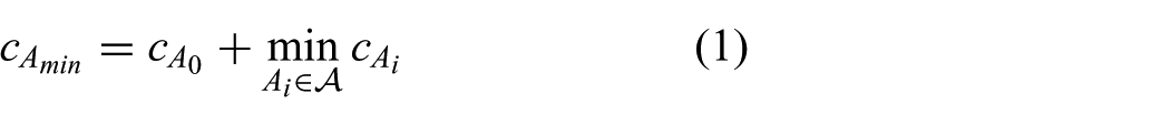
Setup of pairwise comparison for sequential lookahead planning. Given the path cost distributions, we can directly compute the probability that traveling from Start to Goal through A will ultimately yield a cheaper path than traveling via B.
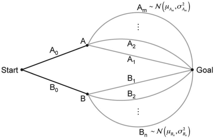
Similar statements can be made for path sets
That is, transitioning to vertex V results in a higher probability of executing a lower cost path than transitioning to any other neighboring vertex
4. RAGS
4.1. Quantifying path risk
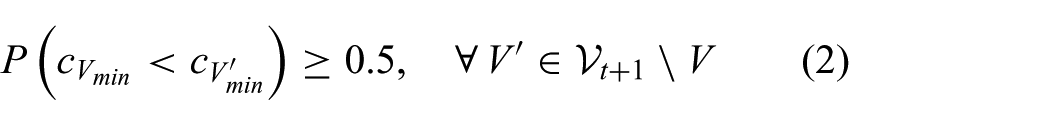
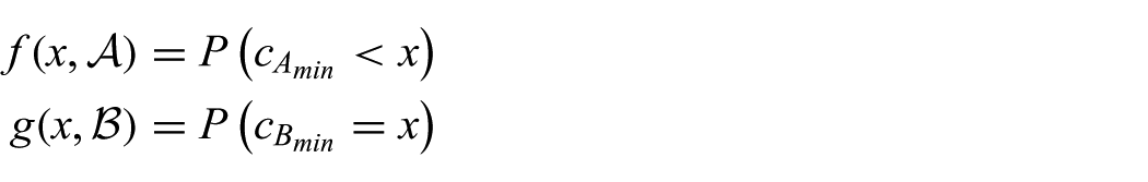
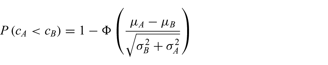
The pairwise comparison
We can now express each term in the integral according to the path cost distributions of each respective set. Let,
As each of the path costs are drawn from normal distributions, then
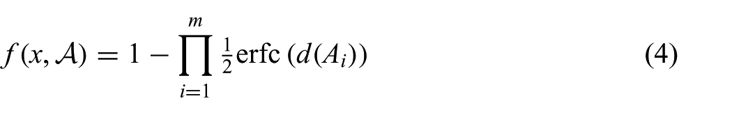
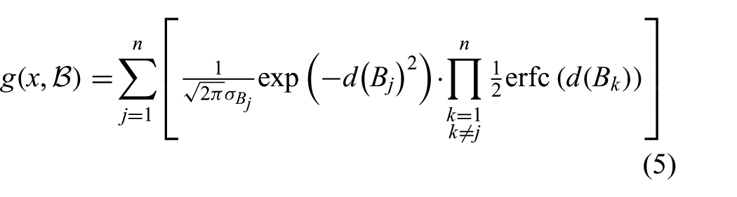
where
As an aside, note that

confirming that these two events are indeed complementary.
Equations (4) and (5) give some intuitive insight into the calculation of path risk. This formulation performs a trade-off between the number of available paths in each set and the quality of the paths in each set, the latter represented by the means and variances of the path cost distributions. For example,
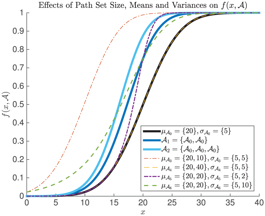
Plot of
Other trends can be observed when adding paths of varying cost distributions to the set. Here
This analysis motivates a bounding approach that compares the values of path cost means and variances to retain only the most relevant paths for the calculation of Equation (3). Bounding the path set is especially desirable since the computation of each pairwise comparison has complexity
4.2. Non-dominated path set
Existing graph search algorithms, such as A*, use a total ordering of vertices based on the calculated cost-to-arrive to find a single optimal path between defined start and goal vertices. In contrast, an implementation of RAGS requires two sweeps of the graph, because an initial pass is required to gather cost-to-go information at each node for quantifying the path risk at execution. If all possible acyclic paths between start and goal are to be considered, then this initial pass is exponential in the average branching factor of the search tree. To reduce this computation, we introduce a partial ordering condition based on the path cost means and variances to sort the priority queue and terminate the search. This bounds the set of resultant paths to be considered during execution by accepting only those that exhibit desirable path cost mean and variance characteristics.
As discussed in Section 4.1, the addition of paths with higher mean costs to the existing path set results in little improvement in the overall risk of committing to that set. Similarly, adding paths with higher variances on the path cost results in a slower convergence of
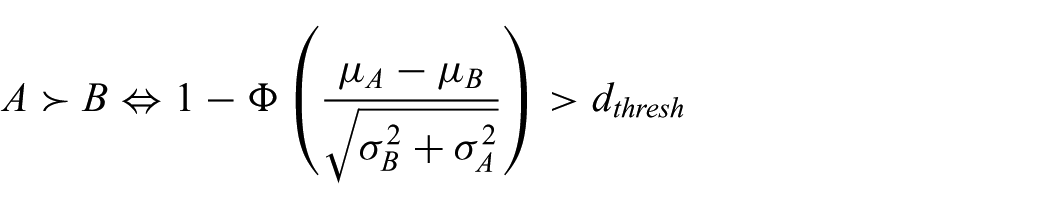
In practice, the partial ordering considers whether a path is dominated by an existing path, either in the open or closed set. For any two paths, A and B, between the same set of start and end vertices, we can consider the probability that the cost of traversing A is lower than the cost of traversing B,

As both path costs are represented by normal distributions, then
where
Expanding
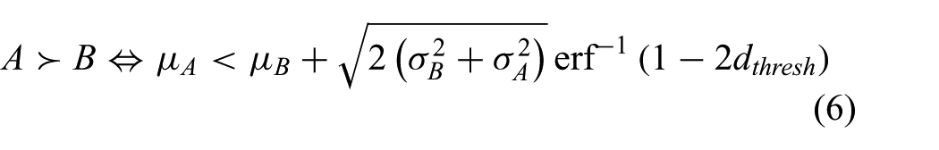
The inverse error function term in Equation (6) produces a value between
Proof. Proof by contradiction: If
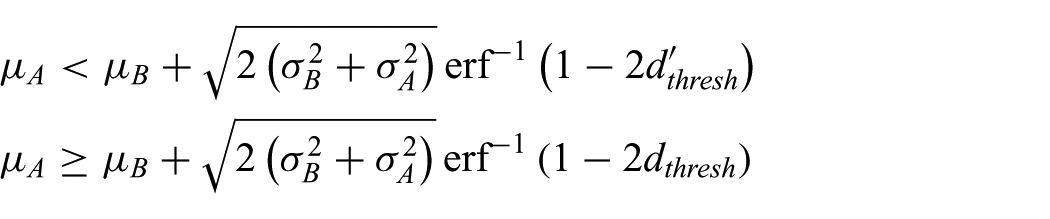
This gives

As

which contradicts the required condition. □
Proof. Let path B be the A* path calculated on the mean, which has the lowest total mean cost,
From a practical perspective, the purpose of the domination threshold is to determine the cutoff point for deciding which paths are included in the non-dominated path set and which are excluded. For example, with a domination threshold of 0.6, all paths in the non-dominated set have at least a
4.3. RAGS dynamic execution
Given the non-dominated path set, path execution can occur by conducting edge transitions at each node to select the path set of least risk according to Equation (2). The true edge transition costs, which become available for all neighboring edges to the current node, are included by directly substituting the known value of
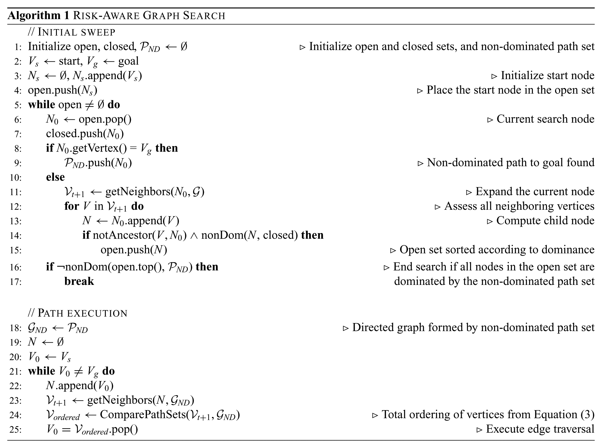
The initial sweep, shown in lines 1–17 of Algorithm 1, is similar to the A* procedure with three notable exceptions. First, in lines 8 and 9, if the current node contains a path from start to goal, then it is included in the non-dominated path set. Second, in line 14, each child node of the current expanded node is checked against the ancestor list to explicitly exclude looping paths. Furthermore, a child node is also excluded at this point if it is found to be dominated by any node in the closed set with the same end vertex. Third, in line 16, the initial sweep is terminated either when open set is empty or when the next node to be expanded from the open set is found to be dominated by any node in the current non-dominated path set.
The RAGS online execution begins by constructing the directed graph formed by the non-dominated path set (line 18). Beginning at the start vertex (line 20), each edge transition first considers the set of all neighboring vertices (line 23), and computes a total ordering of the possible traversals according to Equation 3 (line 24). It is here that RAGS incorporates the observed costs of the next transitions if that information is available. The edge traversal to the best vertex from this set is executed (line 25), and this loop continues until the goal vertex is reached.
5. Comparison with existing search algorithms
We compared RAGS against a naïve A* implementation, a sampled A* method, and a greedy approach. Naïve A* finds and executes the lowest-cost path based on the mean edge costs and does not perform any replanning. The greedy search is performed over the set of non-dominated paths and selects the cheapest edge to traverse at each step. The sampled A* method searches over graphs constructed by sampling over the edge cost distributions and executes the path that is most frequently found. To provide a fair comparison, the planning time of sampled A* (related to the number of sampled graphs it plans over before selecting the most frequent path) is limited to the time RAGS needed to find a path. We chose A* to compare against as a simplified solution to the problem and sampled A* because the method was previously introduced in a similar domain (Murphy and Newman, 2013). The greedy approach provides a baseline for comparison to a purely reactive implementation.
The search algorithms were tested on a set of graphs generated with a uniform random distribution of 100 vertices over a space
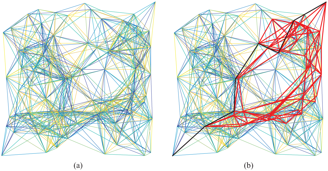
A sample search graph is shown in (a). The mean cost is the sum of the Euclidean distance plus a random additional cost. Edge variances are represented using a scale from blue to yellow on the graph. The darker (more blue) the edges, the less variance there is on the cost. The non-dominated path set (red) and the executed RAGS path (black) shown in (b) demonstrate the algorithm’s ability to account for both the path cost distributions as well as the available path options to goal. Not only does it favor traversing edges with balanced mean costs and variances, it also trades off against the number of remaining path options to the goal. Best viewed in color.
In Figure 4, we show the resulting path costs for 100 trials over a single graph configuration, where each trial drew new edge costs from the distributions as described above. For this set of experiments RAGS used a domination threshold of
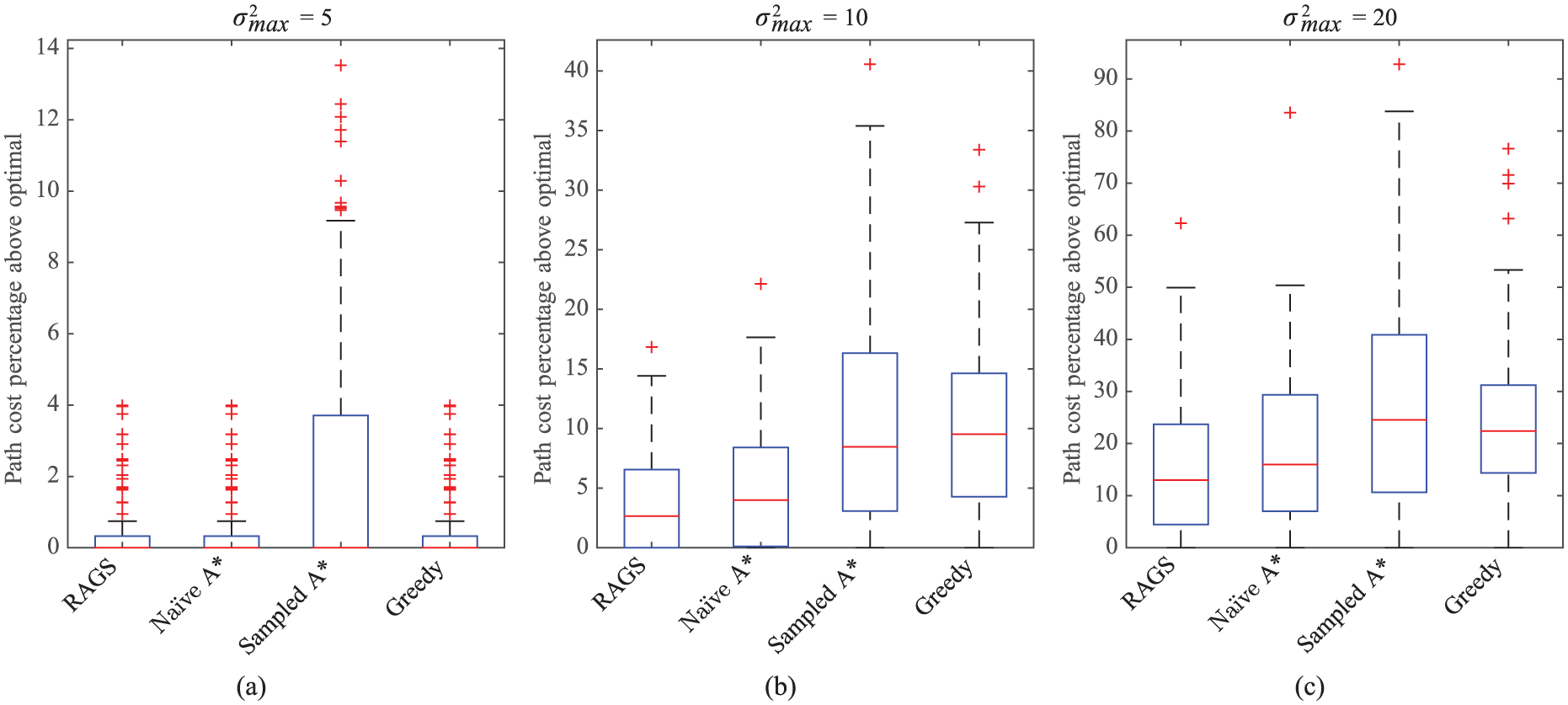
Path search results over 100 samples of one graph configuration (unique vertices and mean edge costs); edge cost variances are drawn uniformly between 0 and
The sampled A* approach can account for variability in costs along the edges as long as it can sample enough paths. However, similar to naïve A*, this method is also prone to risky paths that yield high-cost outliers because it cannot incorporate dynamic local information in the way that RAGS does. In fact, for this set of trials, sampled A* produced the poorest path choices compared to all other methods. This is partly because the domination threshold for these trials was set relatively low, and so the number of equivalent Monte Carlo graphs used by sampled A* was also relatively low.
The collated results from 100 unique graph configurations, with each graph sampled 100 times, are shown in Figure 5. Figure 5a shows the final path cost performance for a range of domination threshold values,
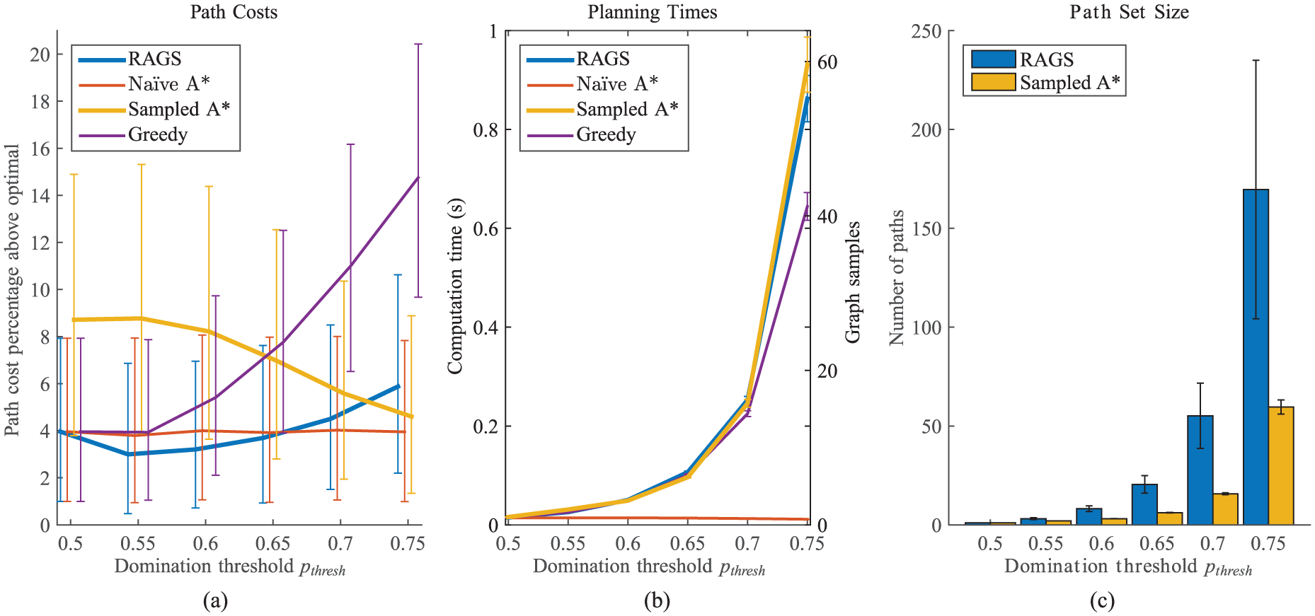
(a) Final median path cost performance, (b) computation times, and (c) path set size across varying domination thresholds for
Figure 5b shows the path search and execution times for each method and the total number of Monte Carlo graph queries performed by sampled A*. Graph search and execution was calculated on a 2.1 GHz Intel® CoreTM i7-3612QM laptop. The computation time for the greedy planning method on the non-dominated path set closely follows that of RAGS, indicating that the majority of the computation cost is incurred during the initial sweep rather than during the online path execution. As expected, the computation time for A* planning is stable and the number of Monte Carlo graphs queried by sampled A* is proportional to the RAGS computation time. By comparing Figures 5a and 5b, we can see that sampled A* requires over 50 Monte Carlo samples of the graph to improve upon the performance of RAGS.
The number of paths stored in the non-dominated path set for increasing
6. Satellite data experiments
We also applied RAGS to a real-world domain using satellite data. In robotic path planning there is often prior information available on the environment, but this information is not necessarily reliable. An example of this is using overhead satellite imagery to provide prior information for path planning. In these trials, we collected and filtered satellite images to identify potential obstacles for a low-flying unmanned aerial vehicle (UAV). To convert the image into a useful mapping of obstacles, we filtered the satellite images to identify trees. The filtering process begins by applying a Gaussian filter to locally homogenize the images. Then the trees were extracted from the filtered images based upon pixel color; an example satellite image input and the resulting obstacles are shown in Figures 6a and 6b.
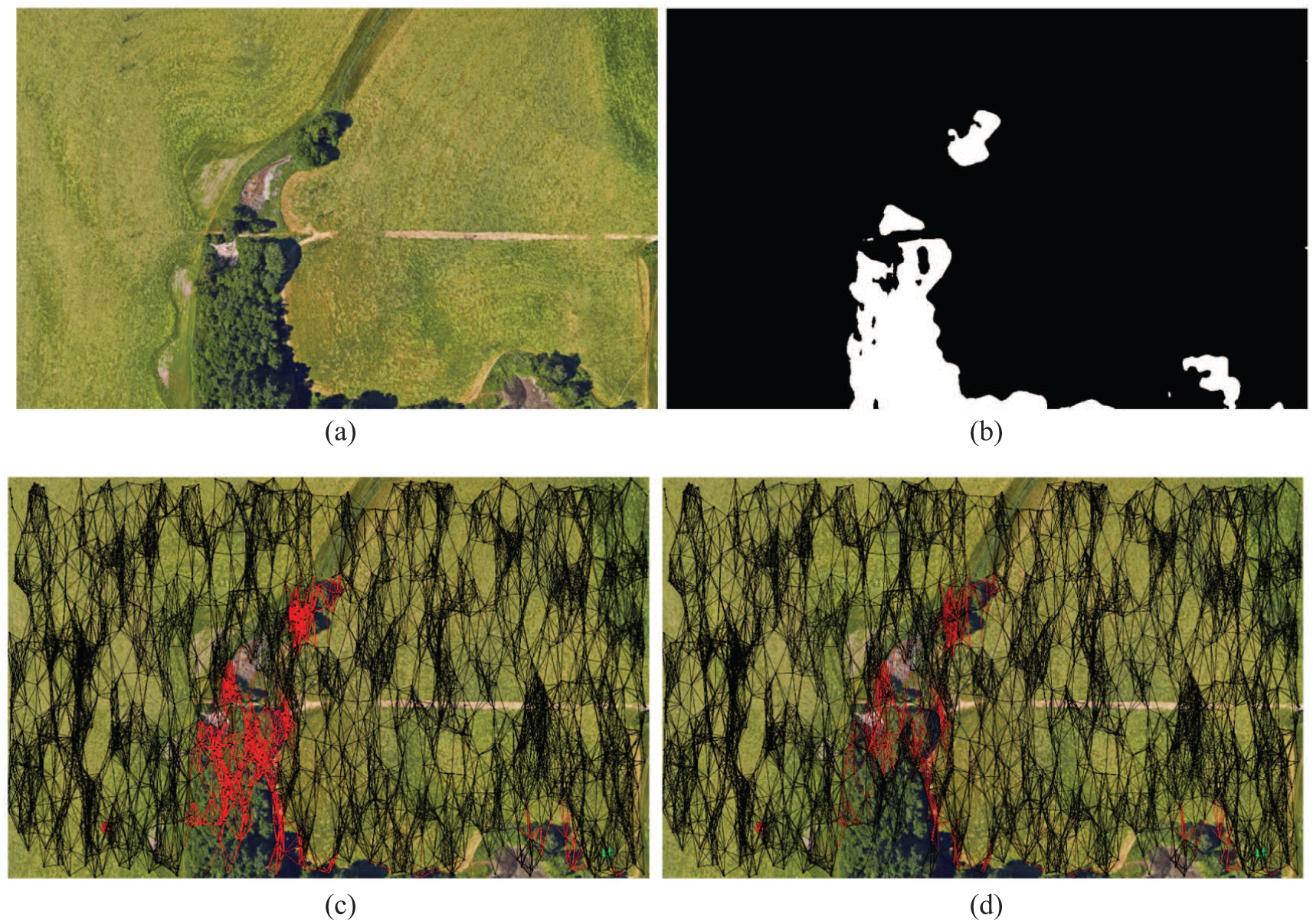
An example of a raw satellite image (a) and the extracted obstacles shown in white (b). The mean estimated obstacle edge costs (c) and variance (d) for the raw satellite image in Figure 6a. Lower values are black and higher values transition to red, best viewed in color.
After the filtering process, the images provided a rough estimate of obstacles that could force the vehicle to slow down or alter its path. Unfortunately, due to the resolution of the satellite imagery, limitations of the tree/obstacle filter, and temporal differences between when the images were taken, the satellite imagery cannot be used to provide a guaranteed cost to traverse an area. For example, the obstacle detection cannot determine the height of the detected trees to determine if the UAV can fly above them or will be forced to detour around them. Consequently, the imagery can only be used as an estimate of the obstacles in the environment and the additional costs the obstacles will add to the flight path. Using the same method as before, we randomly sampled the space to generate a connected graph of flight paths. To estimate the costs of flight paths we calculated the mean and variance of the detected obstacle pixels over each edge and used these values to characterize the edge cost distributions. This process was then repeated for every edge in the graph. Example graph means and variances are shown in Figures 6c and 6d. The mean pixel lightness of the obstacle map along an edge was used to scale the Euclidean distance to generate mean edge costs. This was used to represent a penalty for the increased likelihood of an obstacle and a slower flight speed. The variance in pixel lightness across an edge in the obstacle map was directly used as the edge cost variance in our calculations. After the edges were assigned distributions, RAGS with
6.1. Results
We compared the performance of RAGS with the three other planning algorithms across 96 satellite images. The images are of fields with trees of varying tree densities and may also contain houses or other built structures. Images were captured at different resolutions as well as at different altitudes. The majority of the data have tree clusters scattered throughout the image to provide interesting path-planning dilemmas. Four distinct environments are shown in Figures 7, 8, 9, and 10. To avoid visual clutter, only the RAGS, A*, and hindsight optimal paths are shown here. The hindsight optimal path contains no notion of risk and is calculated solely on the “true” edge traversal costs, which are not observable to the planners until they reach a neighboring node. As in the previous experiments in Section 5, for each sample of an image, we draw the true costs from the computed distributions and use these to evaluate the executed paths of each planner. Compiled results for all four planning algorithms on the satellite imagery dataset are presented in Figure 11.
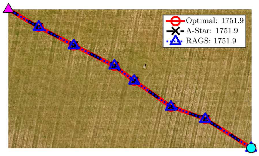
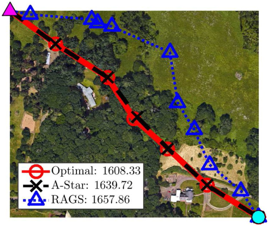
The RAGS, A*, and the global optimal (known only in hindsight) paths with the final path costs. The goal is to traverse from the top left start vertex to the bottom right goal vertex. The empty field is a test case showing that both algorithms plan direct paths as expected in an obstacle-free environment. Note that although only the final executed RAGS path is shown, the entire non-dominated path set is considered during the online traversal.
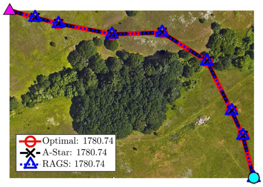
Test case demonstrating that both A* and RAGS plan an intuitive path in the presence of obstacles. The planners remain in the empty fields for the duration of the path and only enter the forest briefly as expected.
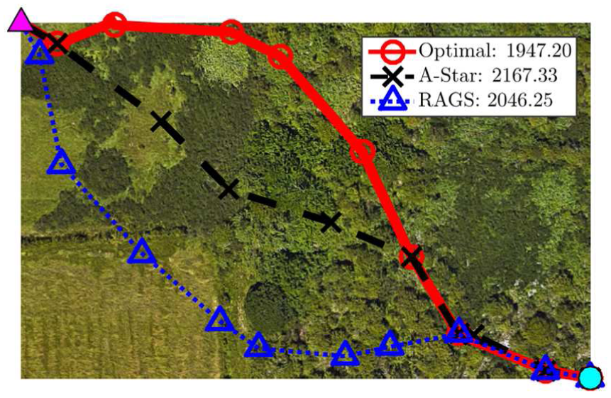
The RAGS path traveling through an initial cluster of trees to take full advantage of the clear route over the open field. In contrast, A* finds a path that attempts to navigate straight to the goal through the dense forest without consideration of the cost variability of that region. The costs after execution show that the RAGS path is actually cheaper due to balancing the risk of finding a path through the initial tree cluster that connects to a less-risky path to goal. This demonstrates the benefit of RAGS, knowing when to take risks and when to act conservatively.
Paths planned through a dense cluster of trees surrounding the goal. Here we can see RAGS plans around the cluster, where the path is ultimately shorter but has a higher risk, before traversing through a less-cluttered area. RAGS takes advantage of the wide open region instead of searching for narrow tracks within the tree cluster.
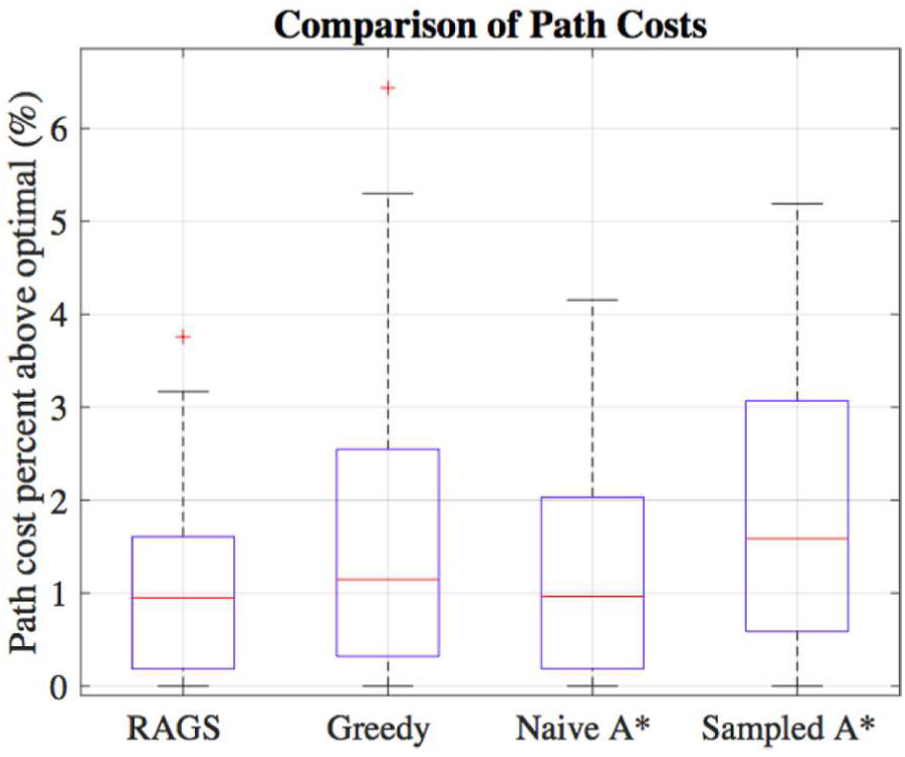
Results from satellite data experiments, using 100 samples of 96 images. Box plots represent the path cost percentage above what would have been, in hindsight, the optimal path. The same trends in performance are seen as with the simulated graphs. By accounting for the uncertainties in travel cost, RAGS is able to reduce the risk of executing expensive paths.
In Figure 7, the paths through an empty field are straight from start (magenta triangle) to goal (cyan circle). As expected, there is little variance in edge costs across the open field, and the trajectories for RAGS and A* are identical and follow the optimal path. In Figure 8 the two planners, RAGS and A*, again follow identical paths in the presence of an obstacle field with limited options. This map results in one obvious intuitive path for the planners to find and demonstrates their ability to plan a trajectory around obstacles.
Analyzing the paths found in Figure 9 is more interesting than the previous two examples. Here we start to see the benefit of RAGS in obstacle-dense environments. The path from start to goal is blocked by large clusters of semi-permeable forest. A* executes a path through the center of the cluster that has a low cost in the mean but does not allow for easy deviations if the path is found to be untraversable. On the other hand, the path executed by RAGS demonstrates the non-myopic nature of this algorithm. RAGS executes a path that travels around the main cluster to minimize the portion of the path within the dense section of the forest. The executed path balances the risk of traversing high-cost edges at the start and end of the path with the benefit of exploiting the sections of open field in the bottom left. Although the RAGS path length is longer than the A* path, it ultimately achieves a lower total cost. Values are drawn from the edge distributions to calculate what would have been the optimal path in hindsight. The optimal path (known only after execution) is shown in red, and we can see that it also avoids the center route executed by A*.
The final test case can be seen in Figure 10, here A* actually outperforms RAGS. In this test case the hindsight-optimal and A* path is to push through the center of the cluster along edges with potentially higher penalties, but a shorter Euclidean distance. The RAGS planner alternatively takes a path that largely avoids the cluster along a safer, although ultimately slightly higher-cost, path.
The compiled results for all tested algorithms are shown in a box plot of percentage above the hindsight optimal in Figure 11. From the comparison on the three randomly generated graphs in Section 4.3, we showed that the relative performance of RAGS increases as edge variance increases. This is accounted for by the fact that the other planning algorithms are merely searching over the single heuristic of mean traversal cost. If variance is low then this can be enough to solve for a path that is close to the optimal solution. However, Figure 11 reveals that real-world datasets can contain significant noise, and it is valuable to account for that variability during planning.
7. Flight trials
In addition to the satellite data experiments, the RAGS planner was tested on a quadrotor traversing through an unstructured wooded environment. The quadrotor is provided a graph representation of the environment, consisting of the edge cost distributions calculated from satellite imagery of the area. It then uses either A* to plan a route, or RAGS to generate the non-dominated path set, from the start to finish locations. The goal of the quadrotor is to fly to the finish location as quickly as possible while avoiding obstacles in the environment and following either the A* or RAGS path, the latter of which is updated online given sensor feedback. The quadrotor uses on-board sensing and computing to plan its trajectory, detect and avoid obstacles, and re-plan as needed autonomously and in real time while navigating the path.
The quadrotor used in these experiments is the DJI Matrice M100 equipped with a ZED RGBD camera
3
and Nvidia Jetson TX2 Development Board,
4
as shown in Figure 12.
5
The Jetson TX2 uses Ubuntu 16.04 and Robot-Operating System (ROS) Kinetic-Kame.
6
The motion of the Matrice is restricted to a 2D plane by controlling the Matrice to a fixed altitude of 10 m above ground level. The Matrice’s heading is controlled to orient the ZED RGBD camera in the direction of travel; effectively always facing the Matrice forward. The ZED’s depth image, accessed via the ZED-ROS-wrapper,
7
is used to detect obstacles at the quadrotor’s operating altitude. As obstacles are detected, they are inflated and added to a 2D occupancy map at 100 Hz. The Matrice then uses the ROS navigation package to plan a path in the 2D occupancy map from the Matrice’s current location to the next goal vertex in the A* or RAGS route at
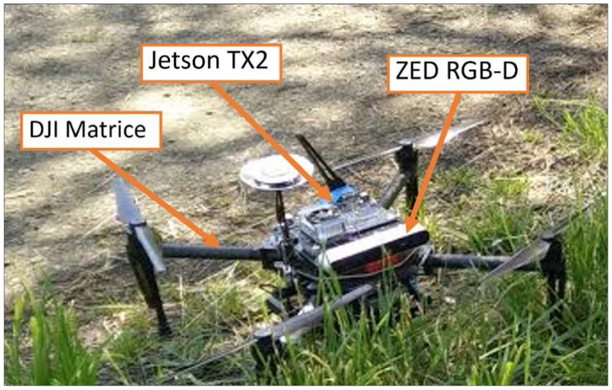
The DJI Matrice M100 used in the hardware trials.
The movement of the Matrice is controlled at 50 Hz using proportional–derivative controllers for heading, altitude, and horizontal velocities to follow the path to the next vertex. The DJI on-board ROS SDK 8 is used to acquire positioning information and control the motion of the Matrice. The Matrice’s horizontal velocity is determined by the mean distance reading in the platform’s operating plane. In an open environment with few obstacles, the Matrice’s velocity increases. As more obstacles are detected and become closer to the Matrice, the platform slows down. Using this method, the Matrice controller guides the platform along the path between vertices. When it reaches a distance within 3 m of the intermediate goal vertex, the Matrice queries either the A* or RAGS on-board planner for the next vertex and repeats this process.
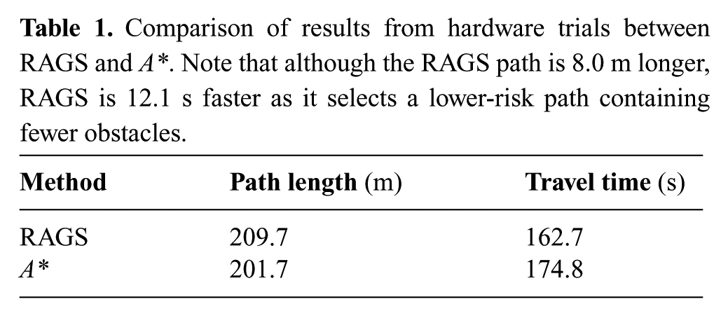
The hardware experiments were conducted in the unstructured wooded environment shown in Figure 13. This environment was chosen because it provides multiple paths from the start location, green triangle, to the goal location, red circle. The length of the trial was constrained by the limited battery life of the Matrice and the foot speed of the safety pilot. As seen in Figure 13 the Matrice executed different paths for the RAGS and A* planners, metrics are provided in Table 1. The RAGS planner took the slightly longer path, 209.7 m compared with 201.7 m for the A* path. However, the RAGS path can be seen to be less risky, with fewer nearby obstacles, which allowed the quadrotor to travel at a faster speed. The Matrice was able to complete the RAGS path in 162.7 s, compared with the A* path, which was completed in 174.8 s. The time and distance reported is from when the Matrice autonomously departs the starting vertex and autonomously reaches within 3 m of the goal vertex. See Extension 1 for a video of the flight trial.
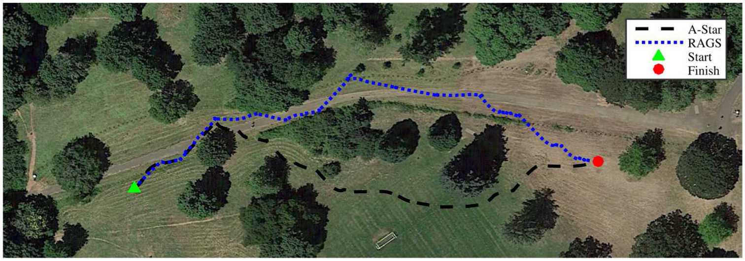
The paths taken in the hardware trials by the Matrice for the RAGS and A* planners. The RAGS path is slightly longer, 209.7 m, compared with the A* path, 201.7 m. However, the RAGS path allowed for a slightly higher travel speed and was completed in 162.7 s compared with the 174.8 s taken along the A* path. Note that although the RAGS path is 8.0 m longer than the A* path, it is completed 12.1 s faster. This is because the RAGS planner accounts for risk along the path and chooses a path from the non-dominated set with fewer obstacles, allowing the quadrotor to travel at a higher speed.
Comparison of results from hardware trials between RAGS and A*. Note that although the RAGS path is 8.0 m longer, RAGS is 12.1 s faster as it selects a lower-risk path containing fewer obstacles.
We note that this experiment serves as a case study of the performance of RAGS and does not represent a statistically meaningful result. However, it does confirm a number of properties of the algorithm in a real-world field trial. First, these hardware trials verify that the RAGS algorithm can be run online in real time on existing hardware in an unstructured environment. Second, it confirms both the trends found in the simulations, that RAGS will attempt to mitigate risk by choosing a safer path, and our own intuition about how the RAGS algorithm should perform, i.e. it chooses the uncluttered path along the road over the shorter path through the trees, which is qualitatively safer and easier for the vehicle to traverse.
8. Conclusion
In this paper, we have introduced a novel approach to incorporating and addressing uncertainty in planning problems. The proposed RAGS algorithm combines traditional deterministic search techniques with risk-aware planning. RAGS is able to trade off the number of future path options, as well as the mean and variance of the associated path cost distributions to make online edge traversal decisions that minimize the risk of executing a high-cost path. The algorithm has been compared against existing graph search techniques on a set of graphs with randomly assigned edge costs, as well as over a set of graphs with traversability costs generated from satellite imagery data. In all cases, RAGS has been shown to reduce the probability of executing high-cost paths over A*, sampled A*, and a greedy planning approach.
In addition to simulation experiments, we have also implemented the RAGS algorithm in a hardware demonstration on board a DJI Matrice M100 platform equipped with a ZED RGBD camera. Our experiments compared the A* and RAGS flight trajectories and showed that although the RAGS planner selected a longer path, the Matrice was able to complete the full RAGS trajectory in shorter time than the A* trajectory. RAGS traded off a slightly longer path to maintain greater distance to the nearest obstacles. As a result, the Matrice was able to fly the RAGS path at faster speeds compared with flying the A* path when the platform needed to slow down and maneuver around obstacles.
Our RAGS code is available open source at https://github.com/osurdml/RAGS.
8.1. Future work
In this work, we have experimented on graphs with edge costs represented by normal distributions. However, the RAGS framework is designed to accommodate any edge cost distribution function. Indeed one argument against using normal distributions to represent costs in path-planning problems is that they result in non-zero probabilities for sampling negative values. Thus, they may be a poor representation of the true cost distribution. Other distributions, such as the log-normal or beta distributions, may be more accurate. However, computing the non-dominated path set and the pairwise comparisons for general distributions is a non-trivial task that is worth further investigation.
Another promising extension of this work is to consider RAGS as applied to planning for information optimization. In this case, edge cost probability distributions would represent environmental information, and paths would be generated based on the amount of information the vehicle may collect in different parts of the map. The foreseen challenges of this work will be to manage the changes in expected information gain on-the-fly in a principled manner, since properties such as submodularity of the data will mean that future observations downstream no longer reap the gains expected at the start. We believe that incorporating information theoretic planning into the RAGS framework could potentially lead to wider applications in probabilistic planning.
Footnotes
Appendix. Index to multimedia extensions
Archives of IJRR multimedia extensions published prior to 2014 can be found at http://www.ijrr.org, after 2014 all videos are available on the IJRR YouTube channel at http://www.youtube.com/user/ijrrmultimedia
RAGS flight demo
Funding
The author(s) disclosed receipt of the following financial support for the research, authorship, and/or publication of this article: This research was conducted at Oregon State University and has been funded in part by NASA (grant number NNX14AI10G) and the Office of Naval Research (grant numbers N00014-14-1-0509 and N00014-17-1-2581).