A dataset of daily interactive manipulation

Abstract

Robots that succeed in factories may struggle to complete even the simplest daily task that humans take for granted, because the change of environment makes the task exceedingly difficult. Aiming to teach robots to perform daily interactive manipulation in a changing environment using human demonstrations, we collected our own data of interactive manipulation. The dataset focuses on the position, orientation, force, and torque of objects manipulated in daily tasks. The dataset includes 1,603 trials of 32 types of daily motions and 1,596 trials of pouring alone, as well as helper code. We present our dataset to facilitate the research on task-oriented interactive manipulation.

Keywords

Dataset interactive manipulation force motion tracking

1. Introduction

Robots excel in manufacturing environments that require repetitive motion with little fluctuation between trials. In contrast, humans rarely complete any daily task by repeating exactly what was done last time, because the environment might have changed. We aim to teach robots daily manipulation tasks using human demonstrations so that they are able to fulfill them in a changing environment. To learn how humans finish a task by manipulating an object and interacting with the environment, we need three-dimensional (3D) motion data of the objects involved in fine manipulation motions, and data that represent the interaction.

Most of the currently available motion data are in the form of vision data, i.e., RGB videos and depth sequences (for example, Das et al., 2013; Fathi et al., 2012, 2011; Kuehne et al., 2014; Rogez et al., 2014; Rohrbach et al., 2012; Shimada et al., 2013), which are of little or no direct use for our purpose. Nevertheless, certain datasets exist that do include motion data. The Slice & Dice dataset (Pham and Olivier, 2009) includes three-axis acceleration of cooking utensils that are used while salads and sandwiches are prepared. The 50 Salad dataset (Stein and McKenna, 2013) includes three-axis acceleration of more cooking utensils than the Slice & Dice dataset, which are involved in salad preparation. The Carnegie Mellon University multimodal activity (CMU-MMAC) dataset (de la Torre et al., 2009) includes motion capture and six-degree-of-freedom (6-DoF) inertial measurement unit (IMU) data of human subjects making dishes. The IMUs record acceleration in ( $x, y, z$ , yaw, pitch, roll). The Actions-of-Making-Cereal dataset (Pieropan et al., 2014) includes 6-DoF pose trajectories of the objects involved in making cereal that are estimated from RGB-D videos. The TUM Kitchen dataset (Tenorth et al., 2009) includes motion capture data of human subjects setting tables. The OPPORTUNITY dataset (Roggen et al., 2010) includes 3D acceleration and 2D rotational velocity of objects. The Wrist-Worn-Accelerometer dataset (Bruno et al., 2014) includes three-axis acceleration of the wrist while the subject is performing daily activities. The Kinodynamic dataset (Pham et al., 2018) includes mass, inertia, linear and angular acceleration, angular velocity, and orientation of the objects, but the manipulation exists in its own right and does not serve to finish a task.

The aforementioned datasets are less than ideal in that: (1) calculating the position trajectory using the acceleration may be inaccurate owing to accumulated error; (2) the motions of objects are not always emphasized or even available; and (3) all the activities are not fine manipulations that serve to finish tasks. Having identified those deficiencies, we collected a dataset ourselves that includes 3D position and orientation (PO), force and torque (FT) data of tools/objects being manipulated to fulfill certain tasks. The dataset is potentially suitable for learning either motion (Huang and Sun, 2015) or force (Lin et al., 2012) from demonstration, recognizing geometric constraints (Subramani et al., 2018), motion classification (Aronson et al., 2017) and understanding (Aksoy et al., 2011; Flanagan et al., 2006; Paulius et al., 2018; Soechting and Flanders, 2008), and is potentially beneficial to grasp research (Lin and Sun, 2015a,b, 2016; Sun et al., 2016).

2. Overview

We present a dataset of daily interactive manipulation that can be accessed at http://rpal.cse.usf.edu/datasets_manipulation.html. Specifically, we record daily performed fine motion in which an object is manipulated to interact with another object. We refer to the person who executes the motion as the subject, the manipulated object as the tool, and the object interacted with as the object. We focus on recording the motion of the tool. In some cases, we also record the motion of the object.

The dataset consists of two parts. The first part contains 1,603 trials that cover 32 types of motions. We choose fine motions that people commonly perform in daily life that involve interaction with a variety of objects. We reviewed existing motion-related datasets (Bianchi et al., 2016; Huang et al., 2016; Huang and Sun, 2016) to help us decide which motions to collect.

The second part contains the pouring motion alone. We collect it to help with motion generalization to different environments. We chose pouring because: (1) pouring is found to be the second most frequently executed motion in cooking, right after pick-and-place (Paulius et al., 2016); and (2) we can vary the environment setup of the pouring motion easily by switching different materials, cups, and containers. The pouring data contain 1,596 trials of pouring 3 materials from 6 cups into 10 containers.

We collect the two parts of the data using the same system. We specifically describe the pouring data in Section 10.

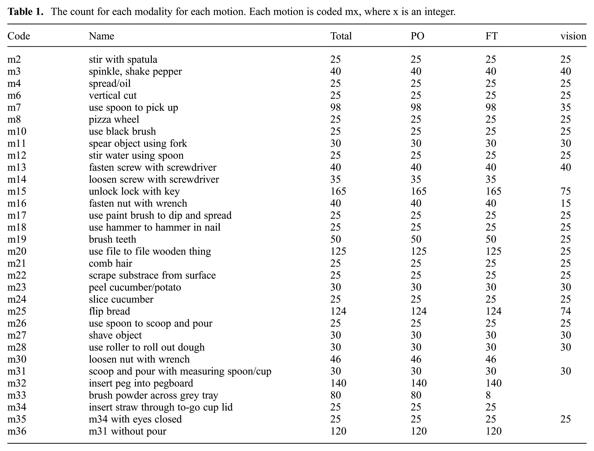
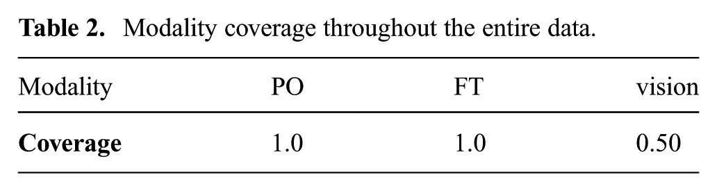
The dataset aims to provide PO and FT, but also provides RGB and depth vision data with a smaller coverage. Table 1 shows the number of trials and the counts of each modality for each motion. The minimum number of trials for each motion is 25. Table 2 shows the coverage of each modality throughout the entire data, where the coverage has a range of $(0, 1]$ , and a coverage of 1 means the modality is available for every trial. The lower coverage of the vision modality is due to filming permission restriction.

Table 1.

The count for each modality for each motion. Each motion is coded mx, where x is an integer.

Code	Name	Total	PO	FT	vision
m2	stir with spatula	25	25	25	25
m3	spinkle, shake pepper	40	40	40	40
m4	spread/oil	25	25	25	25
m6	vertical cut	25	25	25	25
m7	use spoon to pick up	98	98	98	35
m8	pizza wheel	25	25	25	25
m10	use black brush	25	25	25	25
m11	spear object using fork	30	30	30	30
m12	stir water using spoon	25	25	25	25
m13	fasten screw with screwdriver	40	40	40	40
m14	loosen screw with screwdriver	35	35	35
m15	unlock lock with key	165	165	165	75
m16	fasten nut with wrench	40	40	40	15
m17	use paint brush to dip and spread	25	25	25	25
m18	use hammer to hammer in nail	25	25	25	25
m19	brush teeth	50	50	50	25
m20	use file to file wooden thing	125	125	125	25
m21	comb hair	25	25	25	25
m22	scrape substrace from surface	25	25	25	25
m23	peel cucumber/potato	30	30	30	30
m24	slice cucumber	25	25	25	25
m25	flip bread	124	124	124	74
m26	use spoon to scoop and pour	25	25	25	25
m27	shave object	30	30	30	30
m28	use roller to roll out dough	30	30	30	30
m30	loosen nut with wrench	46	46	46
m31	scoop and pour with measuring spoon/cup	30	30	30	30
m32	insert peg into pegboard	140	140	140
m33	brush powder across grey tray	80	80	8
m34	insert straw through to-go cup lid	25	25	25
m35	m34 with eyes closed	25	25	25	25
m36	m31 without pour	120	120	120

Table 2.

Modality coverage throughout the entire data.

Modality	PO	FT	vision
Coverage	1.0	1.0	0.50

3. Hardware

On a desk surface, we use blue masking tape to enclose a rectangular area that we refer to as the working area, and within which we perform all the motions. We aim a PrimeSense RGB+depth camera at the working area from above.

We started collecting PO data using the OptiTrack motion capture (mocap) system and soon afterwards replaced OptiTrack with the Patriot mocap system. Both systems provide 3D PO data regardless of their difference in technology. Patriot includes a source and a sensor. The source provides the reference frame, with respect to which the PO of the sensor is calculated. We use an ATI Mini40 FT sensor together with the Patriot PO sensor. To attach both the FT sensor and the PO sensor to a tool, we used a cascading structure that can be represented as: (tooltip + adapter + FT sensor + universal handle + PO sensor), where “+" means “connect.” The end result is shown in Figure 1. A tool generally consists of a tooltip and a handle. We disconnected the tooltip from the stock handle, inserted the tooltip into a 3D-printed adapter, and glued them together. Then we connected the adapter to the tooling side of the FT sensor using screws. We 3D-printed a universal handle and connected it to the mounting side of the FT sensor using screws. At the end of the universal handle we mounted the PO sensor using screws. In some cases, we tracked the object in addition to the tool, and to do that we put a second PO sensor on the object, as shown in Figure 2.

Fig. 1.

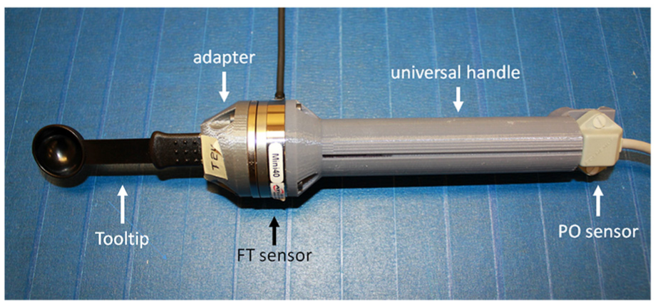
The structure that connects the tool, the FT sensor, and the PO sensor.

Fig. 2.

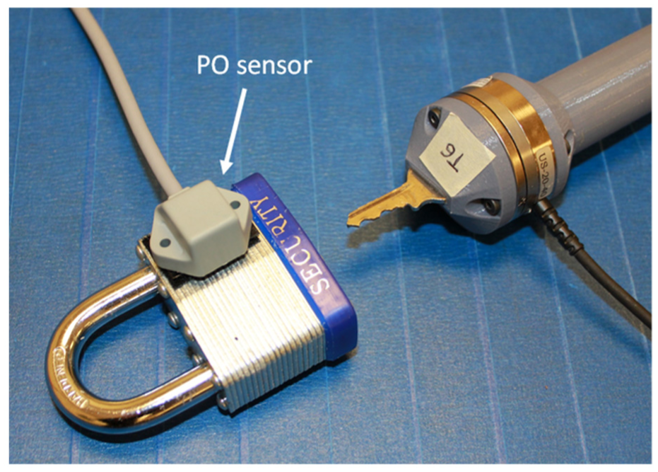
Tracking both the tool and the object with two PO sensors.

Each tooltip is provided with a separate adapter. As the tooltip and the adapter are glued together, a tool is equivalent to “tooltip + adapter.”Figure 3 shows the tools that we have adapted.

Fig. 3.

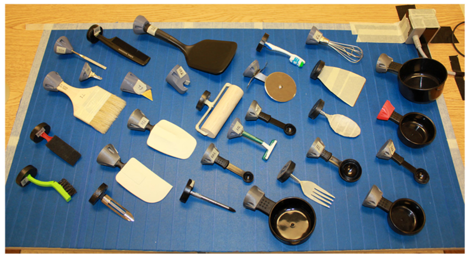
Examples of the tools that we have adapted

4. Coordinate frames

To track a tool using OptiTrack, we need to define the ground plane and define the tool as a trackable. The ground plane is set by aligning a right-angle set tool to the bottom left corner of the working area The trackable is defined from a set of selected markers, and is assigned the same coordinate frame, with the origin being the centroid of the markers. This is shown in Figure 5.

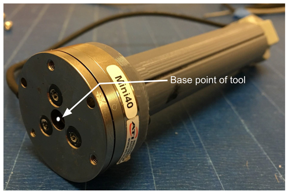
Patriot contains a source that supports up to two sensors. The source provides the reference frame for the sensors as shown in Figure 6. We define the base point of the tool to be the center of the tooling side of the FT sensor, as shown in Figure 4. The translation from the PO sensor to the base point of the tool is $[14.3, 0, 0.7]$ , in the frame of the PO sensor, in units of centimeters.

Fig. 4.

The base point of the tool is the center of the tooling side of the FT sensor.

Fig. 5.

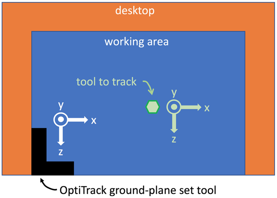
Top view of setting the coordinate frame of the ground plane and the trackable using OptiTrack.

Fig. 6.

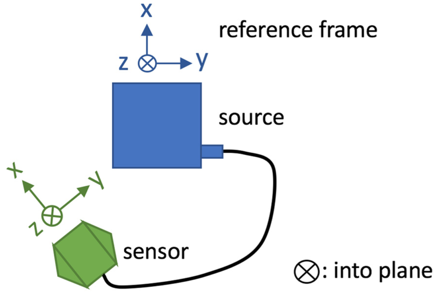
Illustration of the Patriot source and sensor when they are placed on the same plane, and the corresponding coordinate frames. Here ⊗ means into the paper plane.

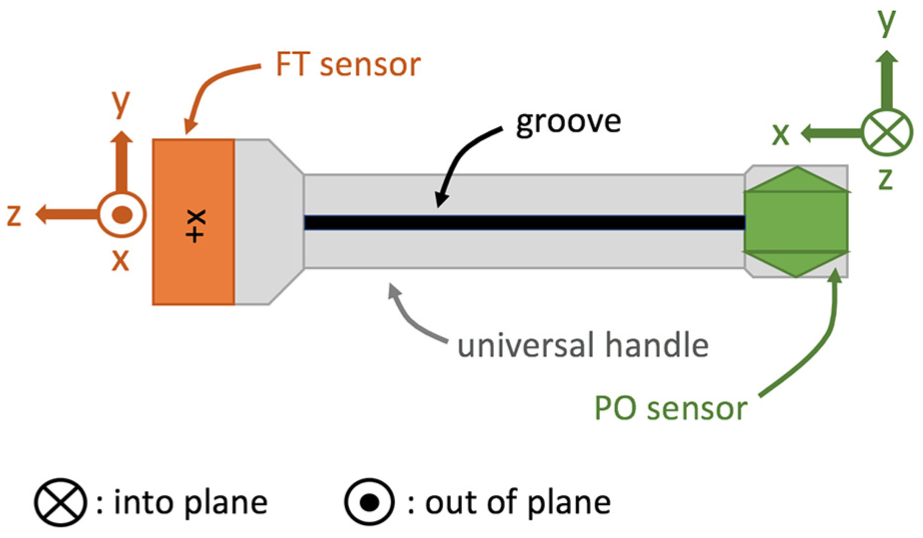
The FT sensor and the PO sensor are connected through the universal handle. The groove on the universal handle is orthogonal to both the $x - y$ plane of the FT sensor and the $y - z$ plane of the PO sensor. The relationship between the local frames of the FT sensor and the PO sensor is shown in Figure 7.

Fig. 7.

Top view of the FT sensor with its local frame, the universal handle, and the PO sensor with its local frame. Here ⊗ means into the paper plane and ⨀ means out of the paper plane.

5. Calibrate FT

Definition 1. The level pose of the universal handle is a pose in which the groove of the handle faces up, and in which the y–z plane of the FT sensor or equivalently the x–y plane of the PO sensor is parallel to the desk surface.

Definition 2. An average sample is the average of 500 FT samples.

The FT sensor has non-zero readings when it is static with the tool installed on it. We calibrate the FT sensor, or make the readings zero, before we collect any data. We hold the handle in a level pose (Definition 1), and take an average sample (Definition 2) which we set as the bias $F T_{b}$ . We subtract the bias from each FT sample before saving the sample: $F T_{t} \leftarrow F T_{t} - F T_{b} .$ We calibrate the FT sensor each time we switch to a new tool.

6. Modality synchronization

Different modalities run at different frequencies and therefore need synchronization, which we achieve by using time stamps. We use Microsoft QueryPerformanceCounter (QPC) to query time stamps with millisecond precision.

When we start the collection system, we query the time stamp and set it as the global start time $t_{0}$ . Then we start each modality as an independent thread, so that they run simultaneously and do not affect each other. For each sample, a modality queries the time stamp t through QPC, and set the difference between t and $t_{0}$ , i.e., the time elapsed since $t_{0}$ as the time stamp for that sample:

t \leftarrow t - t_{0}

(1)

7. Data format

The data are organized in a “motion → subject → trial → data files” hierarchy, as shown in Figure 8, where the prefixes for motion, subject, and trial directories are m, s, and t, respectively.

Fig. 8.

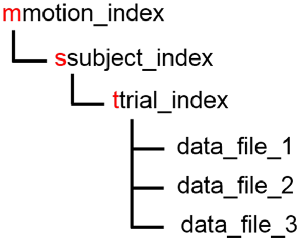
The structure of the dataset where the red text is verbatim.

RGB videos save as . avi, depth images save as . png, and the rest of the data files save as . csv. Both RGB and depth have a resolution of $640 \times 480$ , and are collected at 30 Hz.

The csv files excluding those of OptiTrack follow the same structure as shown in Figure 9. The first row contains the global start time and is the same in all the csv files that belong to the same trial. Starting with the second row, each row is a data sample, of which the first column is the time stamp (Equation (1)), and the rest of the columns are the data specific to a certain modality. The OptiTrack csv file differs in that it contains a single-column row between the start-time row and the data rows, which contains the number of defined trackables (1 or 2). In the following, we explain the data part of a row for each different csv file.

Fig. 9.

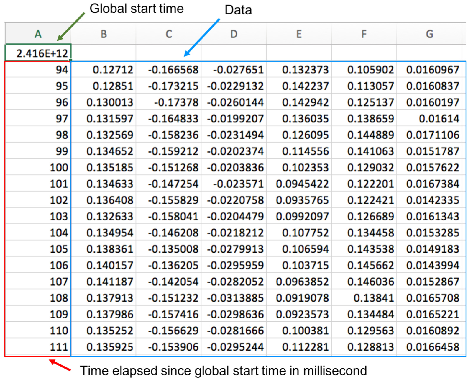
The structure of a non-OptiTrack csv data file.

FT sensor outputs six columns ( $f_{x}, f_{y}, f_{z}, τ_{x}, τ_{y}, τ_{z}$ ), where $f_{x}$ and $τ_{x}$ are the force and torque in the $+ x$ direction, respectively. FT can be sampled at a very high frequency but we set it to be 1 kHz. The force has unit pound (lbf) and the torque has unit pound-foot (lbf-ft).

For the RGB videos and depth image sequences, we provide the time stamp for each frame in a csv file. The data part has one column, which is the frame index.

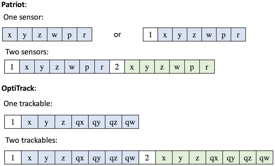
The PO data contain the tool, and may also contain the object. With two PO capture systems, and with or without the object, four different formats exist for the PO data, which are listed in Figure 10. Patriot expresses the orientation using yaw–pitch–roll (w–p–r) as depicted in Figure 11, and OptiTrack uses unit quaternion $(qx, qy, qz, qw)$ . If we only use one trackable but have defined two in OptiTrack, we disable the inactive one by setting all seven columns for that trackable to be $- 1$ , i.e., the eight columns for the inactive trackable would be $(1, - 1, - 1, - 1, - 1, - 1, - 1, - 1)$ .

Fig. 10.

Formats of the columns for PO for one and two sensors.

Fig. 11.

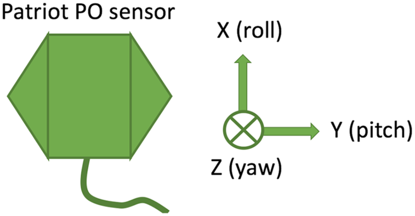
The relationship between the axes and yaw–pitch–roll for the Patriot sensor.

Patriot samples at 60 Hz, its x–y–z has unit centimeter and its yaw-pitch-roll has unit degree. OptiTrack samples at 100 Hz, and its $x - y - z$ has unit meter.

8. Using the data

We provide MATLAB code that visualizes the PO data for OptiTrack as well as Patriot, as shown in Figure 12. The visualizer displays the trail of the base point of the tool (Figure 4) and the object if applicable as the motion is played as an animation in three dimensions. The user can also manually slide through the motion forward or backward and go to a particular frame.

Fig. 12.

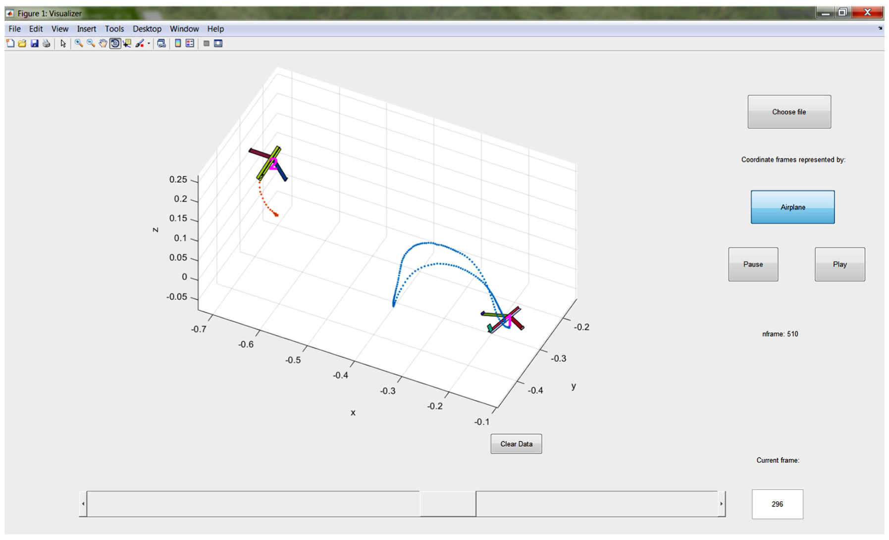
Visualizing the PO data.

The FT and PO csv files have multiple formats, and we provide Python code that extracts FT and PO data from each trial given the path of the root folder. Although we have explained the format of the csv files of the FT and PO data in Section 7, we highly recommend using our code to obtain the FT and PO data to avoid error.

Each modality is sampled at a unique frequency, and using multiple modalities requires using the time stamps. One or more modalities need upsampling or downsampling.

9. Known issue

The PO data recorded using OptiTrack contain occasional flickering and stagnant frames. This is caused by the dependency of OptiTrack on the line of sight. This issue is not present in the data collected with Patriot.

10. The pouring data

We wanted to learn to perform a type of motion from its PO and FT data, and generalize it, i.e., execute it in a different environment. Thus, we need data that show how the motion varies in multiple different environments. We realize that because pouring is the second most frequently executed motion in cooking (Paulius et al., 2016), it is worth learning. In addition, collecting pouring data that contain different environmental setup is easy thanks to the convenience of switching material, cups, and containers. Therefore, we collected the pouring data.

The pouring data include FT, Patriot PO, and RGB videos (no depth). We collected the data using the same system as described above. In the following, we explain what has not been covered and what differs from above.

The physical entities involved in a pouring motion include the material to be poured, the container from which the material is poured, which we refer to as the cup, and the container to which the material is poured which we refer to as the container. The pouring data contain 1,596 trials of pouring water, ice, and beans from 6 different cups to 10 different containers. Cups are considered as tools and are installed on the FT sensor through 3D-printed adapters.

A second PO sensor is taped on the outer surface of the container just below the mouth.

We collected the FT data differently from above. When the cup was empty, we held the handle in a level pose (Definition 1), and took an average sample (Definition 2) that we call “FT_empty.” Then we filled the cup with the material to a desired amount, held the handle in a level pose, and took an average sample that we call “FT_init.” Then we poured, during which we took a number of samples (not average samples) that we call “FT.” After we finished pouring, we held the handle in a level pose, and took an average sample that we call “FT_final.” In summary, we saved four kinds of FT data files: three contain an average sample each, FT_empty, the FT_init, FT_final, and one contains regular samples, FT. We do not consider bias.

The organization of the data is shown in Figure 13.

Fig. 13.

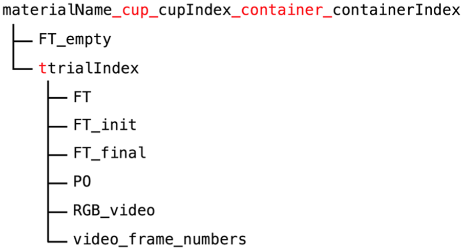
The organization of the pouring data where the red text is verbatim.

The pouring data can be used to learn how to pour in response to the sensed force of the cup. The force is a nonlinear function of the physical properties of the cup and the material, the speed of pouring, the current pouring angle, the amount of material remaining in the cup, as well as other possibly related physical quantities. Huang and Sun (2017) presented an example of modeling such a function using a recurrent neural network and generalizing the pouring skills to unseen cups and containers.

11. Conclusion and future work

We have presented a dataset of daily interactive manipulation. The dataset includes 32 types of motions, and provides PO and FT for every motion trial. In addition, to support motion generalization to different environments, we chose the pouring motion and collected corresponding data. We plan to extend the collection to other types of motions in the future.

Footnotes

Funding

The author(s) disclosed receipt of the following financial support for the research, authorship, and/or publication of this article: This material is based upon work supported by the National Science Foundation (grant numbers 1421418 and 1560761).

References

Aksoy

Abramov

Dörr

Ning

Dellen

Wörgötter

(2011) Learning the semantics of object–action relations by observation. The International Journal of Robotics Research 30(10): 1229–1249.

Aronson

Bhatia

Jia

, et al. (2017) Data-driven classification of screwdriving operations. In: Kulić

Nakamura

Khatib

Venture

(eds.) 2016 International Symposium on Experimental Robotics, pp. 244–253.

Bianchi

Bohg

Sun

(2016) Latest datasets and technologies presented in the workshop on grasping and manipulation datasets. arXiv preprint arXiv:1609.02531.

Bruno

Mastrogiovanni

Sgorbissa

(2014) A public domain dataset for ADL recognition using wrist-placed accelerometers. In: 2014 RO-MAN: The 23rd IEEE International Symposium on Robot and Human Interactive Communication, pp. 738–743.

Das

Doell

Corso

(2013) A thousand frames in just a few words: Lingual description of videos through latent topics and sparse object stitching. In: 2013 IEEE Conference on Computer Vision and Pattern Recognition (CVPR).

de la Torre

Hodgins

Bargteil

, et al. (2009) Guide to the Carnegie Mellon University multimodal activity (CMU-MMAC) database. Technical Report CMU-RI-TR-08-22, Robotics Institute, Carnegie Mellon University.

Fathi

Rehg

(2012) Learning to recognize daily actions using gaze. In: Proceedings of the 12th European Conference on Computer Vision - Volume Part I (ECCV’12), pp. 314–327.

Fathi

Ren

Rehg

(2011) Learning to recognize objects in egocentric activities. In: 2011 IEEE Conference on Computer Vision and Pattern Recognition (CVPR), pp. 3281–3288.

Flanagan

Bowman

Johansson

(2006) Control strategies in object manipulation tasks. Current Opinion in Neurobiology 16(6): 650–659.

10.

Huang

Bianchi

Liarokapis

(2016) Recent data sets on object manipulation: A survey. Big Data 4(4): 197–216.

11.

Huang

Sun

(2015) Generating manipulation trajectory using motion harmonics. In: IROS 2015. IEEE, pp. 4949–4954.

12.

Huang

Sun

(2016) Datasets on object manipulation and interaction: A survey. arXiv preprint arXiv:1607.00442.

13.

Huang

Sun

(2017) Learning to pour. In: 2017 IROS, pp. 7005–7010.

14.

Kuehne

Arslan

Serre

(2014) The language of actions: Recovering the syntax and semantics of goal-directed human activities. In: 2014 IEEE Conference on Computer Vision and Pattern Recognition (CVPR).

15.

Lin

Ren

Clevenger

Sun

(2012) Learning grasping force from demonstration. In: ICRA 2012. IEEE, pp. 1526–1531.

16.

Lin

Sun

(2015a) Grasp planning to maximize task coverage. The International Journal of Robotics Research 34(9): 1195–1210.

17.

Lin

Sun

(2015b) Task-based grasp quality measures for grasp synthesis. In: IROS 2015. IEEE, pp. 485–490.

18.

Lin

Sun

(2016) Task-oriented grasp planning based on disturbance distribution. In: Robotics Research. Berlin: Springer, pp. 577–592.

19.

Paulius

Huang

Milton

Buchanan

Sam

Sun

(2016) Functional object-oriented network for manipulation learning. In: 2016 IROS, pp. 2655–2662.

20.

Paulius

Jelodar

Sun

(2018) Functional object-oriented network: Construction and expansion. In: 2018 ICRA, pp. 1–7.

21.

Pham

Olivier

(2009) Slice&Dice: Recognizing food preparation activities using embedded accelerometers. Berlin: Springer, pp. 34–43.

22.

Pham

Kyriazis

Argyros

Kheddar

(2018) Hand-object contact force estimation from markerless visual tracking. IEEE Transactions on Pattern Analysis and Machine Intelligence 40(12): 2883–2896.

23.

Pieropan

Salvi

Pauwels

Kjellstrom

(2014) Audio–visual classification and detection of human manipulation actions. In: IROS 2014, pp. 3045–3052.

24.

Rogez

III JSS, Khademi

Montiel

JMM

Ramanan

(2014) 3D hand pose detection in egocentric RGB-D images. CoRR abs/1412.0065.

25.

Roggen

Calatroni

Rossi

, et al. (2010) Collecting complex activity datasets in highly rich networked sensor environments. In: 2010 Seventh International Conference on Networked Sensing Systems (INSS), pp. 233–240.

26.

Rohrbach

Amin

Andriluka

Schiele

(2012) A database for fine grained activity detection of cooking activities. In: CVPR 2012.

27.

Shimada

Kondo

Deguchi

Morin

Stern

(2013) Kitchen scene context based gesture recognition: A contest in ICPR2012. In: Advances in Depth Image Analysis and Applications ( Lecture Notes in Computer Science, Vol. 7854). New York: Springer, pp. 168–185.

28.

Soechting

Flanders

(2008) Sensorimotor control of contact force. Current Opinion in Neurobiology 18(6): 565–572.

29.

Stein

McKenna

(2013) Combining embedded accelerometers with computer vision for recognizing food preparation activities. In: Proceedings of the 2013 ACM International Joint Conference on Pervasive and Ubiquitous Computing, pp. 729–738.

30.

Subramani

Gleicher

Zinn

(2018) Recognizing geometric constraints in human demonstrations using force and position signals. IEEE Robotics and Automation Letters 3(2): 1252–1259.

31.

Sun

Lin

Huang

(2016) Robotic grasping for instrument manipulations. In: 2016 13th International Conference on Ubiquitous Robots and Ambient Intelligence (URAI). IEEE, pp. 302–304.

32.

Tenorth

Bandouch

Beetz

(2009) The TUM kitchen data set of everyday manipulation activities for motion tracking and action recognition. In: 2009 IEEE 12th International Conference on Computer Vision Workshops (ICCV Workshops), pp. 1089–1096.