
Abstract
We present a review and reformulation of manifold constrained sampling-based motion planning within a unifying framework, IMACS (implicit manifold configuration space). IMACS enables a broad class of motion planners to plan in the presence of manifold constraints, decoupling the choice of motion planning algorithm and method for constraint adherence into orthogonal choices. We show that implicit configuration spaces defined by constraints can be presented to sampling-based planners by addressing two key fundamental primitives, sampling and local planning, and that IMACS preserves theoretical properties of probabilistic completeness and asymptotic optimality through these primitives. Within IMACS, we implement projection- and continuation-based methods for constraint adherence, and demonstrate the framework on a range of planners with both methods in simulated and realistic scenarios. Our results show that the choice of method for constraint adherence depends on many factors and that novel combinations of planners and methods of constraint adherence can be more effective than previous approaches. Our implementation of IMACS is open source within the Open Motion Planning Library and is easily extended for novel planners and constraint spaces.
Keywords
1. Introduction
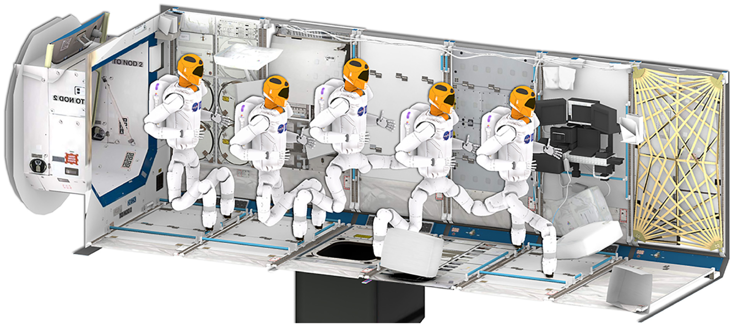
Motion planning is an essential tool for robotic systems. With motion planning, a robot can generate a feasible path given start configurations and goal specifications (Choset et al., 2005). Recently, there has been rapid development in creating robotic systems that are high-dimensional, such as humanoid robots, mobile manipulators, and mechanically redundant arms. Planning for these high-dimensional systems is hard owing to the inherent difficulty of the motion planning problem (LaValle, 2006). In addition, these complex systems face increasingly complex manipulation tasks, which require more information beyond start and goal specifications (some example tasks are shown in Figure 1 for NASA’s Robonaut 2 (Diftler et al., 2011)). For example, consider a robot that must transfer a glass of water; the robot should be constrained to keep the glass level throughout the entire motion. Task constraints encode restrictions on robot motion, and are an important way to concisely specify complex robot motions. Common task constraints include many end-effector constraints and loop-closure constraints, as in parallel manipulators or bi-manual systems carrying an object. An important class of task constraints with special structure are manifold constraints, which encapsulate the examples above as well as many geometric constraints. Planning for complex robotic systems in the presence of manifold constraints is an important and relevant problem as these systems face greater manipulation challenges.
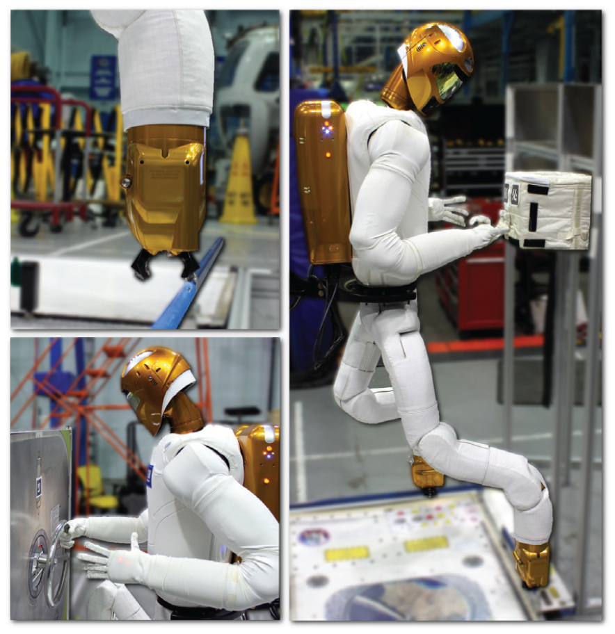
NASA’s Robonaut 2 (R2) executing geometric constrained manipulation tasks. Clockwise from the top-left: R2’s end-effector moves on the Z-axis to grasp a handrail, R2’s legs form a closed chain and a cargo bag is moved linearly from its hold, and R2 turns a valve about its axis.
Sampling-based planners have proven effective at planning motions for high-dimensional systems (Choset et al., 2005). These planners randomly explore the robot’s configuration space and build a discrete representation of valid motions. Many sampling-based planners have been developed with different methods to explore and exploit the valid motions of a robot. However, incorporating manifold constraints in planning is still difficult, as finding configurations that adhere to constraints is a challenging task. Recently, researchers have developed algorithms for planning with manifold constraints that are effective on realistic problems (Berenson et al., 2011b; Jaillet and Porta, 2013b; Kim et al., 2016). Despite their performance, these algorithms are somewhat limited in the sense that they adapt a single sampling-based algorithm to adhere to task constraints by using a specific method for constraint adherence.
1.1. Contributions
The contribution of this paper is a review and reformulation of methods for manifold constrained sampling-based planning within a unifying framework, IMACS (implicit manifold configuration space). IMACS enables a broad class of motion planners to plan in the presence of manifold constraints, decoupling the choice of motion planning algorithm and method for constraint adherence. We provide an open-source implementation of said framework in the Open Motion Planning Library (OMPL) (Şucan et al., 2012), a widely used open-source library for motion planning, and demonstrate its efficacy on complex simulated and real environments.
The key insight of this work is to view geometrically constrained motion planning as an unconstrained planning problem in an implicitly defined, lower-dimensional space. Sampling-based planners are modular and readily adapted to any space or robotic system. IMACS exploits the modularity of the interface between sampling-based planners and the configuration space to decouple the method of constraint adherence from a motion planner. That is, IMACS represents the implicitly defined space with primitives that are necessary for sampling-based planning. In particular, the primitives within the space representation are augmented samplers and local planners, using some method of constraint adherence. We present projection-based (similar to CBiRRT2 (Berenson et al., 2011b)) and continuation-based (similar to AtlasRRT (Jaillet and Porta, 2013b) and TB-RRT (Kim et al., 2016)) methods of constraint adherence as space representations within IMACS.
With IMACS, a broad class of sampling-based planners can use many previously proposed constraint adherence methods and leverage planners and tools developed by the motion planning community. For example, asymptotically optimal planners (Karaman and Frazzoli, 2011), heuristic path optimization (Geraerts and Overmars, 2007), and domain-specific planners for high-dimensional problems (Şucan and Kavraki, 2008) all work without modification in IMACS. IMACS also shows that different methods of constraint adherence can all use the same underlying constraint representation. In addition, we present theoretical results showing that IMACS preserves the probabilistic completeness and asymptotic optimality of sampling-based planners. These theoretical results generalize prior results within the literature. Finally, we demonstrate that different problems can be solved more successfully using novel combinations of planning algorithms and constraint adherence methods compared with existing combinations.
This paper extends the work presented in Kingston et al. (2017). We present a more complete formulation of the algorithms used by the projection- and continuation-based space representations, proofs that the framework preserves probabilistic completeness and asymptotic optimality of sampling-based planners for both the projection- and continuation-based spaces, an open-source implementation of the framework, and additional empirical results including implementation of the framework for NASA’s Robonaut 2.
The organization of this paper is as follows. Section 2 defines constraints, the constrained planning problem, and other mathematical background. Section 3 contains a survey of related work for constrained motion planning. IMACS, our framework which decouples constraints from sampling-based algorithms, is presented in Section 4. Theoretical guarantees of IMACS are presented in Section 5. The implementation of IMACS and empirical results, both in simulated problems and on the real system, are shown and discussed in Section 6. Section 7 contains concluding remarks and directions for future work.
2. Preliminaries
This section presents mathematical background for motion planning under manifold constraints, as well as differentiating our framework from related work described in the next section. We first present the motion planning problem and associated terminology. Next, we introduce manifold constraints, the type of constraints we consider, and how they are represented. Finally, we present the constrained motion planning problem as used in this work.
2.1. Motion planning
This work considers the geometric motion planning problem, or the generalized movers’ problem, which concerns finding a feasible path of a robot that avoids collision with obstacles. Canonically, the robot is viewed as a single point in an abstract space, the configuration space (Lozano-Pérez, 1983). The configuration space, or
For the basic motion planning problem, the robot also needs to avoid some set of obstacles. Obstacles form a closed set
For simplicity of presentation, we consider configurations spaces that are a closed subset of a Euclidean space, i.e.,
2.1.1. Asymptotically optimal motion planning
As discussed in the next section, there has been much recent work on asymptotically optimal motion planning. These algorithms are concerned not only with finding a collision-free path, but also finding a path that is optimal with respect to some cost function
2.2. Manifold constraints
In many cases, avoiding collisions or optimizing a cost function is the only concern for computing a valid path. However, for the constrained motion planning problem presented in this work, we would also like to adhere to some set of constraints on the robot’s motion. In particular, we consider constraints that are functions of the robot’s geometry, constraints that only use the robot’s current configuration
We define constraints as constraint functions
We say that F is adhered to when
As F is a concatenation of at least
We assume that
Thus, the problem of constrained motion planning results in finding a path in an implicitly defined constrained configuration space:

Importantly, as constraint functions are smooth and have a Jacobian of full rank when
The fact that
This representation of constraints encompasses a broad set of constraints as presented in the literature. For example, consider a simple point robot in
Manifold constraints are also known as holonomic constraints (Latombe, 1991; Laumond, 1986), as they are integrable functions of the robot’s configurations. Note that holonomic constraints do not fundamentally change the motion planning problem. Sometimes, the structure of constraints allows for direct reparameterization. One type of constraint that allows for reparameterization are explicit constraints: constraints that explicitly determine the value of some configuration parameters, e.g., a manipulator grasping an object determines the objects configuration from the manipulator’s forward kinematics. Under explicit constraints, the dependent configuration parameters are not necessary. Another example of reparameterization is any articulated robot. Typically, articulated robots are parameterized by their joint angles. It is also possible to model an articulated robot as a constrained system: each of the links of the manipulator is a free-flying rigid body (with
Differential geometry is core to the representation used in this work, which can broadly be described as the study of smooth manifolds with some geometric structure. A comprehensive overview can be found in Spivak (1999) and Lee (2003). Additional definitions are provided in Sections 4 and 5 as needed.
2.3. Volume-reducing constraints
In this work, we do not discuss constraints other than manifold constraints in detail. A brief discussion of volume-reducing constraints and their relation to the methods presented in this article is given here.
Closely related to manifold constraints are volume-reducing constraints, or inequality constraints. These are constraints of the form

This volume either is of non-zero volume or is empty due to being unsatisfiable. For some regions of non-zero volume, rejection sampling and standard unconstrained planning techniques can be used. This is similar to what is done in some constrained sampling-based techniques that “inflate” the manifold into a volume by loosening the tolerance
3. Related work
In this work, we study sampling-based planning in the presence of manifold task constraints. There is a wide breadth of literature concerning techniques to plan motions, represent constraints, and adhere to constraints. Using task constraints to specify the motion of a robotic system has its roots within industrial control (Khatib, 1987; Mason, 1981). Task constraints on robot motion can be used to specify many useful manipulation tasks (Siméon et al., 2004), generate valid motion for parallel manipulators and closed chains (LaValle, 2006; Tsai, 1999), and even model proteins in structural biology (Zhang and Hauser 2013).
The first applications of geometric constraints to planning in low-dimensional spaces were reduced to problems of finding geodesics on polyhedral structures (Mitchell et al., 1987), similar to finding shortest paths of visibility graphs (Alexopoulos and Griffin, 1992; Asano et al., 1985). Most early work with task constraints did not focus on geometric constraints and was directed at non-holonomic constraints, such as differential drive cars (Barraquand and Latombe, 1993). However, as planners were applied to more complex high-dimensional systems with more interesting manipulation tasks, geometric constraints were revisited as a difficult addition to the motion planning problem; constraints within higher dimensions (particularly those for articulated mechanisms) require specialized constraint adherence techniques.
3.1. Other methods
While not the focus of this paper, a short survey of other methods for planning in the presence of manifold constraints is given for completeness.
For end-effector constraints, one approach is to plan a path for the end-effector, so constraints can be directly evaluated and adhering poses can be sampled. After planning a path within the workspace, a corresponding path in the robot’s configuration space is generated using inverse kinematics (IK) (James et al., 2015; Rakita et al., 2018; Sentis and Khatib, 2005). However, these methods may not be efficient as re-planning is required if a computed path cannot be mapped into the configuration space of the robot. Completeness is also not guaranteed unless all feasible IK solutions can be generated from any given constraint. In addition, if multiple end-effector constraints are placed upon the system, null-space projection methods (Sentis and Khatib, 2005) will not yield a probabilistically complete algorithm.
Another approach that operates within the robot’s workspace is IK-based reactive control, which uses convex optimization to find constraint adhering motions, e.g., those used at the DARPA Robotics Challenge (Atkeson et al., 2015; Fallon et al., 2015; Johnson et al., 2015). While effective with operator supervision, these controllers are usually incomplete and are prone to reaching local minima created by the interaction of the objective function and constraints. As local controllers are optimization-based methods, hard geometric constraints are relaxed into soft cost-based constraints, and invalid motions can be generated.
Trajectory optimization approaches (e.g., Schulman et al., 2014; Zucker et al., 2013) optimize within trajectory space and are effective for everyday manipulation tasks, but suffer from many of the same shortfalls as reactive control. However, trajectory optimization methods can generate motions that adhere to task constraints by either adding the constraint as a penalty to optimization objective or as an equality constraint. Recently, Bonalli et al. (2019) presented a method for trajectory optimization on an implicitly defined manifold. No comprehensive comparison of constrained non-sampling-based methods to sampling-based methods exists, and a thorough analysis is outside the scope of this paper.
3.2. Sampling-based planning
The key idea of sampling-based planning is to avoid computing the free configuration space
Multi-query methods construct a “roadmap” within the configuration space that can be queried multiple times. Single-query methods build a tree of motions rooted from the start or goal. Many techniques perform a bidirectional search for efficiency (e.g., Kuffner and LaValle, 2000) or use coverage estimates to bias search towards unexplored space (e.g., Şucan and Kavraki, 2008). For a more in-depth review of sampling-based planning see Choset et al. (2005), LaValle (2006), Elbanhawi and Simic (2014), and Kavraki and LaValle (2016).
3.2.1. Asymptotically optimal sampling-based planning
While sampling-based planners have been shown to be very efficient in finding feasible paths, paths often have poor quality with respect to a given cost function. One approach to improve path quality is to post-process and locally optimize paths with heuristic methods (Geraerts and Overmars, 2007) or a trajectory optimization-based approach (Dai et al., 2018). Sampling-based algorithms can also provide asymptotic optimality guarantees (Gammell et al., 2015; Janson et al., 2015; Karaman and Frazzoli, 2011). These methods guarantee that the solution path converges to a globally optimal path for a given cost function. If the connection radius is greater than the threshold, then asymptotic optimality is guaranteed. Note that, in practice, smoothing and post-processing techniques typically generate solutions comparable to paths from asymptotically optimal planners (Luna et al., 2013; Luo and Hauser, 2014).
3.3. Constrained sampling-based planning
Constraints introduce a new element of difficulty to the problem: configurations must adhere to the constraint function. The approaches to handling constraints within a sampling-based framework can be organized into a spectrum of the complexity used to compute adhering configurations. As described in Section 2, the constraint function implicitly defines a manifold within the configuration space. The method of constraint adherence is the way a particular method copes with planning in this lower-dimensional space. For this paper, of particular importance are projection- and continuation-based methods.
Projection: Finding configurations that adhere to the constraint function
Continuation: From a known adhering configuration, a tangent space of the implicit manifold can be generated. Adhering configurations and valid local motions can be generated by applying projection to configurations sampled within the tangent space. Tangent spaces can be composed together to create a piecewise-linear approximation of the manifold, or a continuation. This approximation can then be used for sampling adhering configurations or for local planning.
A more detailed survey of constrained motion planning techniques along with other classes of methods can be found in Kingston et al. (2018).
3.3.1 Projection-based methods
In a constrained motion planning problem, a path only contains configurations that adhere to the constraint function. Projection-based methods use a projection operator to find adhering configurations starting from potentially invalid configurations, defined formally in Section 4.2.
The first projection methods capable of solving constrained problems dealt with specialized cases of constraints: specifically, loop closures in parallel manipulators. Planning for loop-closure problems in robotics was first solved with PRM variants using active/passive chain methods (Cortés et al., 2002; Han and Amato, 2000; Yakey et al., 2001), and were also relevant in structural biology (Wedemeyer and Scheraga, 1999). Active/passive chain methods use IK as a projection operator to join the passive chain to the active chain, closing the loop and creating an adhering configuration. Typically, IK algorithms are numerical methods that require computation of manipulator Jacobian (pseudo-)inverses, but methods such as cyclic-coordinate descent (Canutescu and Dunbrack, 2003) and FABRIK (Aristidou and Lasenby, 2011) are Jacobian free.
The idea of projection to adhere to constraints was applied to general end-effector constraints in Yao and Gupta (2005). Task-constrained RRT (Stilman, 2010) further generalized the idea of constraints and utilized Jacobian gradient descent (Buss, 2004) for projection. More recently, CBiRRT2 (Berenson et al., 2011b) and the motion planner implemented for the Humanoid Path Planner (HPP) system (Mirabel et al., 2016) utilize projection with general constraints and can solve complex combinations of constraints. HPP combines explicit constraints and implicit manifold constraints into a more effective and efficient projection routine (Mirabel and Lamiraux, 2018).
Projection methods have been extended to find low-cost paths GradienT-RRT (Berenson et al., 2011a) (note that this is not an asymptotically optimal motion planner), and to asymptotically optimal planners (albeit without formal guarantees) in Jaillet and Porta (2013a). We show how IMACS emulates projection-based methods (such as CBiRRT2 and other previous approaches) in Section 4.2.
3.3.2. Continuation-based methods
Projection, while effective at adhering to constraints, utilizes very little information from the constraint. It is possible to locally approximate the manifold defined by the constraint using a tangent space of an adhering configuration. In this case, the tangent space is a chart of the manifold, locally parameterizing the neighborhood around a configuration. The tangent space can be used to generate new configurations that are close to the manifold, and close to the original adhering configuration. As the complexity of the constraint manifold approximation increases, sampling in the tangent space becomes more accurate at the price of increased computational cost per sample.
Projection from tangent spaces was utilized within the work of Yakey et al. (2001) to generate nearby samples, which are then projected to adhere to the constraint. Tangent spaces have been used by Weghe et al. (2007) and Stilman (2010) for manipulators under general end-effector constraints. The technique has also seen many applications in curve tracking constraints for redundant manipulators (Cefalo et al., 2013; Oriolo and Vendittelli, 2009; Vendittelli and Oriolo, 2009) and structural biology to generate valid motions of proteins with loop closures (Fonseca et al., 2018; Pachov and van den Bedem, 2015; Zhang and Hauser, 2013).
Rather than discarding a tangent space after computation, some methods assemble the collection of tangent spaces into an atlas of the manifold. The atlas is composed of many charts (in this case tangent spaces), a concept borrowed from the definition of differentiable manifolds (Spivak, 1999). To be precise, the atlas is defined as a piece-wise linear approximation of the constraint manifold using tangent spaces, which fully cover the manifold (Henderson, 2002). These methods are derived from numerical continuation techniques, which are designed to compute solutions to nonlinear systems of equations (e.g., the constraint manifold). The key difference between continuation methods (Henderson, 2002) and continuation-based planners is the incremental construction of the atlas interleaved with space exploration, allowing the planner to explore online or reuse results from previous runs.
AtlasRRT (Jaillet and Porta, 2013b) and TB-RRT (Kim et al., 2016) both construct an atlas by incrementally building the set of tangent spaces that approximate the manifold. TB-RRT evaluates the manifold lazily and does not separate tangent spaces, leading to overlap and potential problems with invalid points. AtlasRRT computes halfspaces to separate tangent spaces into tangent polytopes to guarantee uniform coverage in the limit at additional computational cost. AtlasRRT has been extended to an asymptotically optimal algorithm AtlasRRT* (Jaillet and Porta, 2013a) and to kinodynamic planning (Bordalba et al., 2018). Like projection-based methods, both TB-RRT and AtlasRRT are emulated within IMACS, shown in Section 4.3.
3.3.3. Other methods
There are many other approaches to constrained sampling-based planning. One class of methods are reparameterization-based approaches that are similar in spirit to IMACS: they create a new representation of the space that adheres to constraints. However, in the case of “deformation space” (Han et al., 2008) and “reachable volume space” (McMahon, 2016), this representation is an explicit transformation for a particular class of robot and constraint. IMACS, on the other hand, does not explicitly reparameterize the manifold, and instead provides a means of representing the implicitly defined space.
In addition, there are offline sampling-based methods that construct an approximation of the constraint manifold offline. That is, these methods precompute a set of constraint-adhering configurations, and then use this set for sampling and local planning. A general approach for offline computation for online sampling was described in Şucan and Chitta (2012). This kind of approach was employed by Burget et al. (2013) to adhere to balance constraints on a humanoid robot.
3.4. Beyond single constraints
Motion planning with manifold constraints is closely tied to manipulation planning. Manipulation planning, as opposed to motion planning, requires planning a sequence of actions, each of which has different path constraints on the motion of the robot (Siméon et al. 2004). For example, consider a robot that must transfer a cup from one table to another. The robot must approach the cup, pick the cup up, approach the other table, and place the cup down. Each of these motions has different constraints to consider, and are each a constrained planning problem with a different submanifold.
Problems with this structure are multi-modal: continuous motion must switch between different discrete modes of interaction, each mode imposing different constraints on the robot. Multi-modal planning considers planning not just a single submanifold, but on a union of multiple submanifolds. Single-mode planning (i.e., constrained motion planning) is an essential component of a multi-modal planning algorithm. A motion planner within IMACS can be used for single-mode planning.
Hauser and Latombe (2010) addressed the multi-modal planning problem for a finite number of modes, which was extended for infinite modes in Hauser and Ng-Thow-Hing (2011). An asymptotically optimal multi-modal planning algorithm was proposed by Vega-Brown and Roy (2016). In addition, Şucan and Kavraki (2011) implemented multi-modal planning via acyclic task-motion multigraphs, and HPP implements multi-modal planning via constraint graphs (Mirabel et al., 2016). Multi-modal planning is also closely related to task and motion planning, which takes a more hierarchical approach to planning multi-modal paths (Dantam et al., 2018; Garrett et al., 2018; Srivastava et al., 2014).
Another essential component for multi-modal planning is the ability to sample transitions from one mode to the next. This is equivalent to sampling from the manifold defined by the concatenation of the two constraint functions, i.e., the intersection of their manifolds. In Section 5, we show that projection-based sampling covers a manifold defined by a constraint function, and thus can be used as a component in a probabilistically complete manifold sampler. Thus, projection-based sampling can be used as a probabilistically complete transition sampler in multi-modal planning. Note that IMACS only provides components of a multi-modal planner: while single-mode planning and transition sampling are important, they do not form a complete multi-modal planner.
3.5. Software frameworks
There are some software packages available that can perform constrained motion planning, such as the CUIK Suite (Porta et al., 2014) and HPP (Mirabel et al., 2016). However, these are integrated frameworks for robotics that provide specific, specialized constrained motion planning algorithms, rather than the conceptual abstractions in IMACS which allow for mixing and matching of constraint solving techniques and planning algorithms. We provide an implementation of IMACS in OMPL 1.4 (Şucan et al., 2012), discussed further in Section 6.
4. Representing implicit manifolds
Despite their differences, most sampling-based planners have similar requirements from the robot’s configuration space (LaValle, 2006). The capabilities we are concerned with are as follows.
Sampling: Critical to sampling-based planning and exploration is the capability to sample over the entire space or near known configurations.
Local Planning: Typically, sampling-based planners employ a local planner: an efficient, deterministic, and not necessarily complete method that is used to validate whether two states can be connected.
Sampling and local planning, rather than being defined as being planner-specific operations, can be defined as operations on the space itself, and need not be specific to any planner. In general, prior works in geometrically constrained planning have augmented an existing sampling-based planner with some capability to “handle” constraints. More accurately, the augmentations required to craft a constrained motion planner are augmentations of the capabilities as outlined above. The core insight of this work is that, as sampling-based planners plan within an abstract space, augmentation of the space is all that is needed to plan with constraints.
The contribution of this article is a conceptual framework, IMACS, which is outlined within Section 4.1. IMACS enables a broad class of motion planners to plan with constraints, decoupling the choice of motion planner and method of constraint adherence. This section is organized as follows. First we discuss IMACS at an abstract level in Section 4.1 and describe how each of the space primitives are used by a sampling-based planner. The specific way a planner handles these critical components is referred to as the method of constraint adherence, as discussed previously in Section 3.3. Then, we show the two methods for constraint adherence that are implemented within IMACS. The first method we show is a projection-based method in Section 4.2, similar to CBiRRT2 (Berenson et al., 2011b). Next, we show a continuation-based method in Section 4.3, similar to tangent bundle RRT (Kim et al., 2016) and AtlasRRT (Jaillet and Porta, 2013b).
4.1. Implicit manifold configuration space
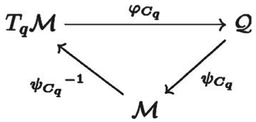
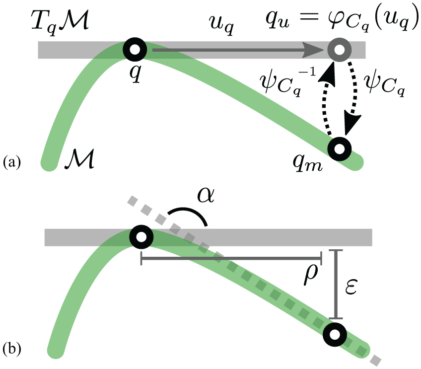
A sampling-based planning algorithm plans within a configuration space, and generates a collision-free path by using a configuration validity checker along with properties of the configuration space, as shown in Figure 2(a). Prior works augmented the planning algorithm with a means of finding constraint adhering motions, as shown in Figure 2(c). In contrast, IMACS is a layer of abstraction that lies between the representation of the robot’s configuration space and the sampling-based planner, as shown in Figure 2(d). IMACS can be thought of as a means to present the implicit manifold
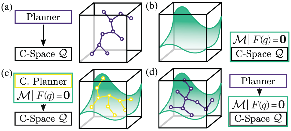
A depiction of the framework and its relation to sampling-based planners. (a) A box configuration space
As discussed above, there are only a few critical components that a sampling-based planner uses from its underlying space. We first discuss metrics and how they are affected within IMACS. Next, we discuss sampling and what properties a sampler should have within IMACS. Finally, we present local planning and interpolation on the constraint manifold within IMACS.
4.1.1. Metrics
Normally, the distance metric utilized by a sampling-based planner is defined by the configuration space. The metric is primarily used for nearest-neighbor computations, by which states near a given state can be found. For example, a point robot in
Thus, prior works generally use the ambient metric from the configuration space, although there has been some work on approximating geodesic distance (Zha et al., 2018). The ambient metric is still “good enough” for most motion planning algorithms in practice, but it is possible that some theoretical guarantees no longer hold. Note that the metric from the configuration space is still a metric within the constraint manifold (when restricted to
4.1.2. Sampling
The ability to sample new configurations in the configuration space is critical to sampling-based planners. This is normally as simple as drawing uniformly random values from
Many sampling-based planners do not use samplers that sample from the entire configuration space (e.g., EST (Hsu et al., 1999) and KPIECE (Şucan and Kavraki, 2008)). Instead, they sample from a neighborhood around a known valid sample, leveraging the intuition that these configurations are likely to be valid as well. We refer to these as neighborhood samplers. These samplers within IMACS must be able to sample (potentially with bias) from a ball of radius r around a known configuration.
Note that many planners (e.g., RRT) do not require samples to be valid, which in the context of constrained motion planning means the configuration is both collision-free and constraint adhering. Thus, the sampler for the ambient configuration space can be used to guide search if samples are not required to be valid.
Several sampling-based planners utilize a “projection” for estimating configuration space coverage in relation to a task (Ladd and Kavraki, 2005; Sánchez and Latombe, 2003; Şucan and Kavraki, 2008), so that the planner can measure sample density and direct sampling towards less-densely sampled regions (note “projection” in this case is not a projection operator as described previously). “Projection” for coverage estimates are problem-specific heuristics to bias sampling and are left unaffected by the IMACS.
4.1.3. Local planning
Local planners are the means for sampling-based planners to quickly and efficiently attempt to find a path between two states. A local planner is not necessarily a complete planner, but typically is fast and deterministic. In geometric planning, the local planner generally takes the form of interpolation along a geodesic between two states. For example, within
For implicit manifolds, traversing geodesics is more complicated. The generated geodesic must be a valid curve in
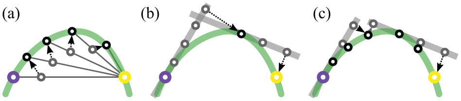
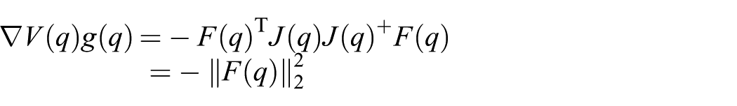
Projection-, tangent bundle-, and atlas-based geodesic interpolation. Between a start (purple) and goal (yellow) points on the implicit manifold (green), the discretized geodesic is computed (black). (a) Projection-based (CBiRRT2). Small extensions are taken (gray) and projected using a projection operator (arrow). (b) Tangent bundle-based (TB-RRT). The manifold is lazily evaluated with tangent spaces (gray), projecting when necessary. (c) Atlas-based (AtlasRRT). Tangent spaces are traversed, projecting at every step.
Within prior constrained sampling-based planning works, generating a geodesic takes the form of taking small enough steps to accurately traverse the manifold’s curvature, creating a discrete geodesic.
Computing the exact geodesic between two points is hard and computationally costly (Hauser, 2013; Mirabel and Lamiraux, 2016). Typically, generating the discrete geodesic takes the form of integrating an ordinary differential equation (ODE) on the surface of the constraint manifold. Given two points

If there is divergence or a lack of progress, then the method terminates unsuccessfully, akin to colliding with an obstacle. However, we show in Section 5.2 that the scheme of ODE integration on manifolds satisfies the criteria of a local planner, and maintains the probabilistic completeness of algorithms running on IMACS.
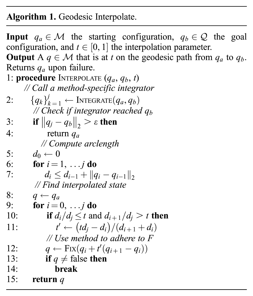
Many sampling-based planners need to compute states interpolated between two states. For example, RRT “steers” toward a sampled state, which in the geometric case means interpolating towards a sampled state up to some fixed distance. However, without the geodesic between two states, it is not known a priori what states lie between two states and where; the geodesic must be computed to interpolate between states. Once a discrete geodesic is computed, an interpolated state can be computed by doing piecewise interpolation, as shown in Algorithm 1. Algorithm 1 first sums distances along the generated geodesic (from an I
4.1.4. Methods for constraint adherence
In summary, the key idea of IMACS is to represent the implicit constraint manifold with primitives that are necessary for sampling-based planning. IMACS consists of a space representation that has augmented sampling and geodesic computation for a given underlying configuration space and constraint. This allows a broad class of sampling-based planners to plan with constraints without any special consideration.
The next two sections describe the approaches to sampling and geodesic computation for the projection-based and continuation-based methods. The projection-based method is similar in concept to CBiRRT2 (Berenson et al., 2011b), but using our constraint function. The continuation-based method is similar to AtlasRRT (Jaillet and Porta, 2013b) and tangent bundle RRT (Kim et al., 2016), and emulates both using shared infrastructure.
4.2. Projection-based method
In a constrained motion planning problem, an adhering path only contains configurations that adhere to the constraint function,
4.2.1. Definitions
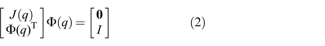
Formally, we define the projection operator as follows.
Given the implicit description of
The formulation of the projection operator as a constrained minimization problem lends itself to a formulation as a Lagrangian with Lagrange multipliers
We can solve for a solution to this system using gradient descent, with the update
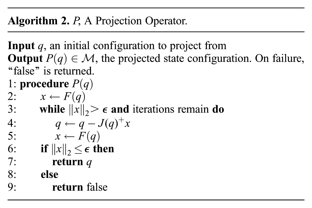
We show in Section 5.1 that the projection operator covers the constraint manifold. That is, for any configuration on the manifold, there exist configurations within the ambient space that will be projected onto the configuration.
4.2.2. Sampling
We assume that the ambient configuration space
Similarly, for sampling nearby existing configurations, the neighborhood sampler from the ambient space is used to sample a new point which is projected to the manifold. Because the constraint manifold uses the ambient metric, all points that are within some distance r to a point in the ambient space are also within r on the manifold.
4.2.3. Local planning
As stated in Section 4.1.3, generating geodesics on the manifold is essential for local planning. For the projection-based local planning, we use a method inspired by integrating an ODE on a manifold (Hairer et al., 2006). In Algorithm 3, we integrate the ODE given in (1) using projection to correct for drift off the manifold. Algorithm 3 uses a fixed maximum step size s with respect to the Euclidean norm, and a tolerance
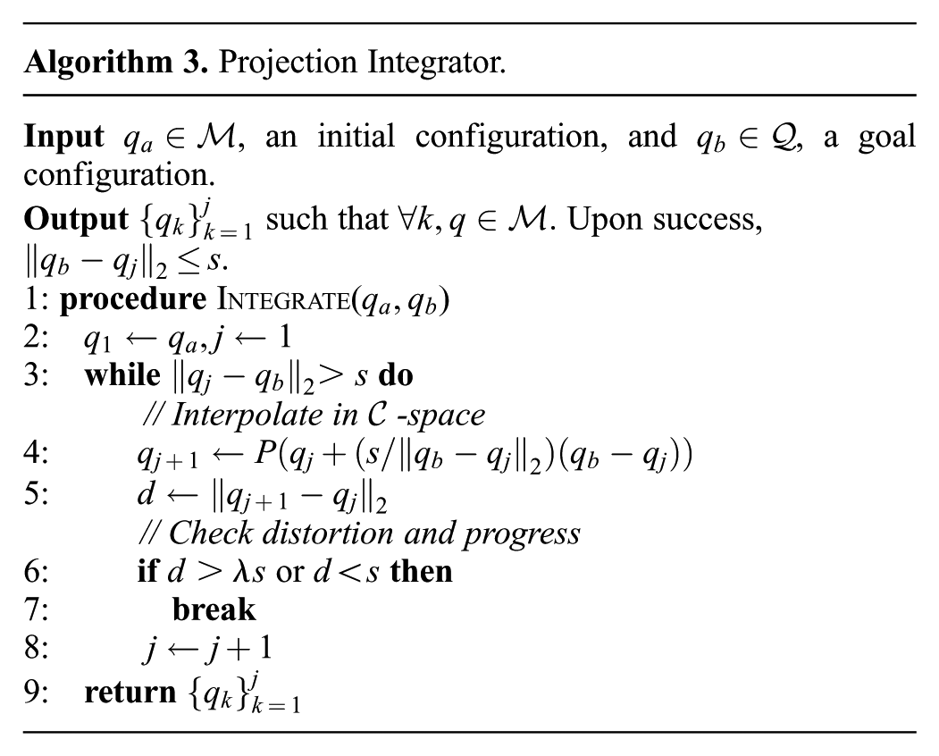
In general, it is not enough to have an arbitrary discrete curve. Continuity must be enforced to some degree. Algorithm 3 is modified slightly from a pure integration approach to respect conditions of continuity in regards to a maximum distortion parameter
4.3. Continuation-based method
As discussed in Section 3.3.2, the constraint manifold
Common between these methods is the construction and maintenance of an atlas. Definitions of the underlying mathematical concepts and implementation of operations associated with the atlas are presented in Section 4.3.1. The definitions and routines presented here are taken and reformulated from Rheinboldt (1996), Henderson (2002), Jaillet and Porta (2013b), and Kim et al. (2016). The primary difference is their use within IMACS as subroutines in a representation of a space, rather than as subroutines within a specific planner.
4.3.1. Definitions
Both AtlasRRT and TB-RRT are higher-dimensional continuation methods: they construct a piecewise-linear approximation of the constraint manifold. This approximation is referred to as an atlas, in reference to the mathematical objective described in the following.
In the case of AtlasRRT and TB-RRT, the atlas is formed of charts that are represented by tangent spaces, which are
Details of how tangent spaces are computed are provided in the following. All together, the collection of tangent spaces at each point on the manifold form the tangent bundle, a vector bundle of tangent spaces.
The following sections describe the various operations that utilize tangent spaces and charts.
A chart is defined by
where
These functions are explained in the following paragraphs.
(a) Illustration of the various chart operators as described in Section 4.3.1. (b) Illustration of the parameters used in a chart’s validity region.
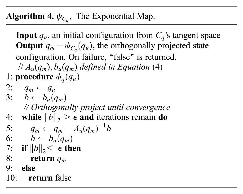
For a given chart around a configuration
Although

This system of equations is solved with gradient descent, shown in Algorithm 4, similar to Algorithm 2. In Algorithm 4, the following equations are used for clarity, given the initial point
Here
The inverse mapping, or logarithmic map,
The following inequalities define the validity region, for a point
These correspond to error, curvature, and maximum span, respectively. These parameters are shown in Figure 4(b). Note that it is possible to adaptively change these parameters, but this is not discussed in this work.
If a point

It is not strictly necessary to separate charts, as will be seen with the tangent bundle planning approach. Each of the charts
In our implementation, the atlas is stored as a collection of charts within a nearest-neighbor structure, using the configuration space’s metric between chart centers. The nearest-neighbor structure is used in Algorithm 5 in the method W
Primarily, all operations that modify or access the atlas are done through G
4.3.2. Sampling
In IMACS, new constraint-adhering configurations are generated by sampling within tangent spaces and projecting these points onto the manifold. A method for sampling the entire manifold and sampling near known configurations is given in Algorithm 6. The method S
Although at first biased towards explored areas, in the limit, once the manifold has been fully explored, sampling approaches uniform sampling (Jaillet and Porta, 2013b). These methods can sample within hard-to-project areas, such as the interior surface of a highly curved manifold. This is empirically demonstrated in Section 6.2.
Neighborhood sampling is shown in N
The validity parameter
4.3.3. Local planning
Generating geodesics using continuation-based methods is also inspired by integrating an ODE on a manifold. In the continuation-based method, geodesic generation is accomplished by walking along the tangent spaces of the approximation, switching tangent spaces once certain criteria are met. In Algorithm 7, two integration methods are shown: I
I
L
4.4. Sampling-based planning
Previously, we have presented the details of how projection- and continuation-based spaces are emulated within IMACS. These spaces are primarily formed by their methods of sampling and geodesic generation. Note that these spaces are not the only methods for constraint adherence that can be captured with IMACS: for example, tangent space-based planning would fit within this framework as well (as described in the first part of Section 3.3.2).
Within the context of sampling-based planning, IMACS is used as the space that a planner is exploring, it is an overlay for an underlying ambient configuration space with a constraint function. Each method for constraint adherence’s sampler is used in place of the sampler normally offered by the ambient configuration space. Note that for some planners (e.g., RRT) the ambient configuration space sampler can be used, as these planners do not directly use samples in their graph construction. Geodesic generation is used in local planning and interpolation: whenever a motion is validated between states or a new state is generated by interpolation, I
We show in Section 5 some of the theoretical guarantees afforded by IMACS. In particular, if a sampling-based planner is probabilistically complete, it remains probabilistically complete while within IMACS. In addition, asymptotically optimal planners such as RRT* and PRM* retain their asymptotic optimality within IMACS.
5. Theoretical guarantees
Many sampling-based planners provide some sort of formal guarantee about their completeness or optimality of solution. Typically, sampling-based planners provide probabilistic completeness guarantees (that is, the probability that a planner will find a solution if one exists goes to 1 as the number of iterations goes to infinity), and many recent planners provide asymptotic optimality guarantees (that is, the solution found will converge to the global optimum as the number of iterations goes to infinity). In this section, we provide building blocks that would compose a larger proof of probabilistic completeness or asymptotic optimality for planners that run within IMACS. These proofs leverage the modular nature of sampling-based planners and provide guarantees about the certain individual components, namely the samplers and local planners.
We first present proofs that show a probabilistically complete planner within IMACS remains probabilistically complete. Samplers and local planners form the core of probabilistic completeness for any motion planner. This is similar to how samplers and local planners form the core of a constrained sampling-based planning method, as well as the core of the methods of constraint adherence within IMACS. The analysis presented follows from the measure theoretic analysis presented in Ladd and Kavraki (2004), which, among other properties of the planner itself, requires two properties from the space representation.
The sampler used must have a non-zero chance of sampling any configuration in the configuration space. For neighborhood samplers, this corresponds to having a non-zero chance of sampling any configuration within the specified radius.
The local planner must be a measurable relation. In addition, the local planner must be such that its transitive closure is a measurable relation (i.e., the path reachability condition). That is, for any two configurations
We show that the samplers and local planners from the projection- and continuation-based methodologies satisfy the above properties, and thus sampling-based planners maintain probabilistic completeness within the framework.
In addition, we provide proofs that asymptotically optimal motion planners maintain their asymptotic optimality guarantees within the framework. We show that under the assumptions above about the sampler and local planner, the proofs of asymptotic optimality of RRT* and PRM* given in Karaman and Frazzoli (2011) hold, and that connection radii
The key intuition of why probabilistic completeness and asymptotic optimality are preserved within IMACS is that the structure of the implicit space is that of a smooth manifold. Manifolds are such that they locally appear to be like a Euclidean space, and thus in a sense are “nice” for planning. It is possible to provide guarantees about sampling and local planning under constraints as, locally, there is always space around the manifold that is well behaved.
The rest of this section is organized as follows. In Section 5.1, we show that projection-based sampling (as defined in Section 4.2.2), which uses a projection operator (as defined in Section 4.2.1), satisfies the criteria of a sampler. Next, Section 5.2 shows that the geodesic generators of the projection- and continuation-based spaces are indeed local planners as defined above. Together, these facts lead to the probabilistic completeness of a planner within IMACS, discussed in Section 5.3. Finally, we discuss how the proofs of asymptotic optimality remain unaffected by IMACS in Section 5.4.
5.1. Manifold coverage and sampling
Key to the projection-based methods is the projection operator. Critically, the projection operator must guarantee that it will project a state onto the constraint manifold. We show that the projection operator, as presented, covers the manifold. That is, we show in Proposition 1 that any open set on the manifold
This proof is inspired by the proof of manifold coverage used in CBiRRT2 (Berenson et al., 2011b) and a proof of continuity of the projection operator given in Mirabel and Lamiraux (2016). However, note that the proof offered in Proposition 1 is more general than the proof of manifold coverage given in Berenson et al. (2011b). The difference lies in the class of constraints considered: Berenson et al. (2011b) gives a proof of manifold coverage for a class of end-effector constraints for manipulators (task space regions), whereas our proof is for any constraint of the form
Recall that we assume the configuration space
We show that the projection operator covers the manifold by showing that there exists a region (potentially small) around the manifold such that all points in this region project onto the manifold. A natural concept for the immediate region closest to the smooth constraint manifold is that of a tubular neighborhood.
A partial tubular neighborhood of
Intuitively, the tubular neighborhood of the manifold can be visualized as “inflating” the manifold, e.g., for a line in
As the manifold is smooth, it makes sense that it can be “inflated” without the tubular region self-intersecting; a smooth manifold can only twist and curve so much, and has no self-intersections. However, note that a manifold can get arbitrarily close to itself, and thus while the tubular neighborhood does exist it can be arbitrarily small. The volume of the tubular neighborhood, and thus the effectiveness of the projection operator, are dependent on the regularity of the constraint function.
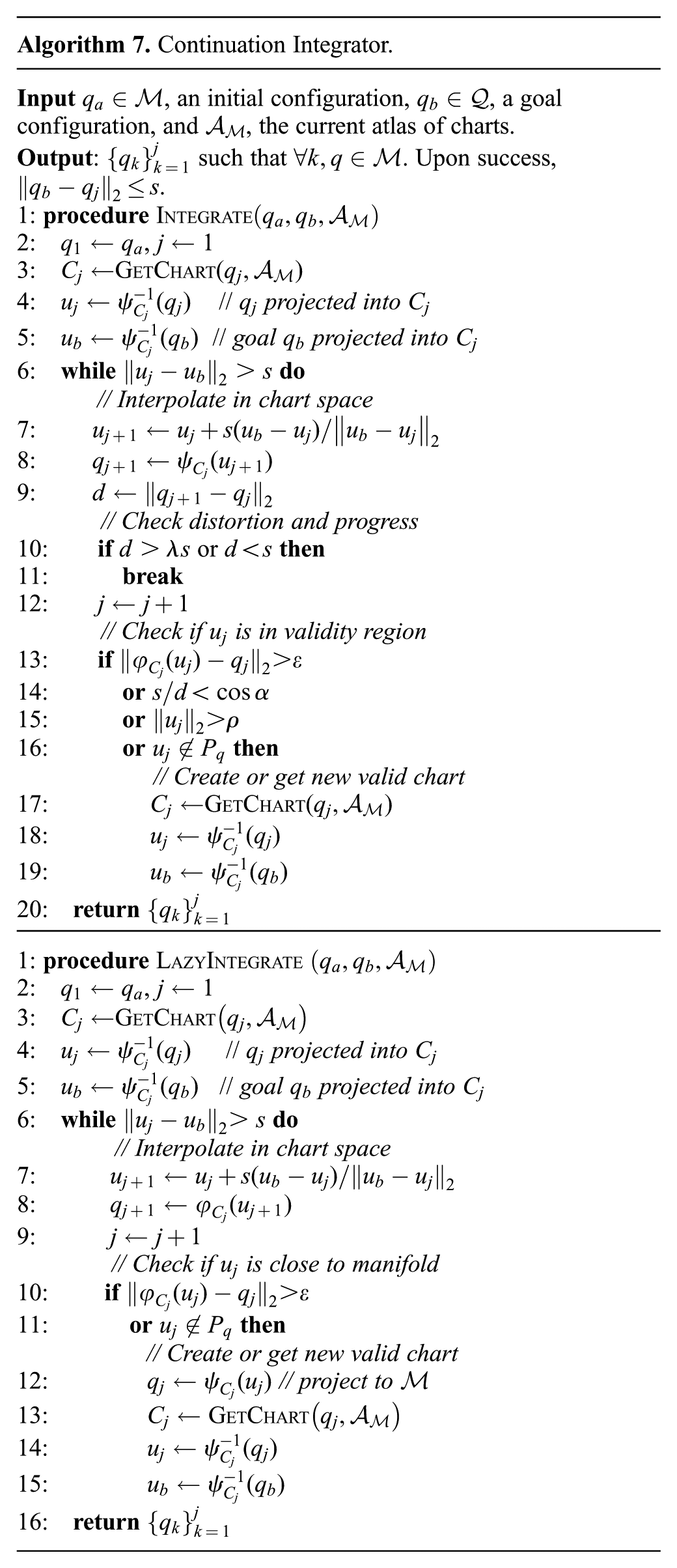
We would like to show that all configurations within this region around the manifold, when projected, end up on the manifold. The gradient descent within the projection operator (Algorithm 2) can be phrased as the flow of an ODE. Thus, we would like to show that, for some desired point on
Lyapunov stable, if for every
asymptotically stable, if
The Lyapunov stability of an equilibrium point can be proven with the Lyapunov’s theorem (Luenberger, 1979). With these tools, we are now ready to prove that the projection operator covers the manifold.
For all
Following from the definition of a projection operator (Definition 6), define an ODE g over the domain Dx:

Note that g is continuous, as F is
Put V, the candidate Lyapunov function as
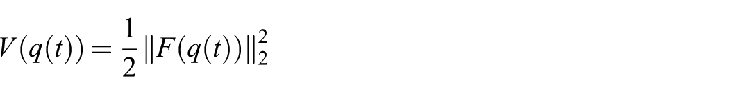
where V is continuous as the norm is a continuous map and g is continuous from above. Here V is also differentiable, with
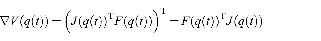
Here V satisfies the properties of the Lyapunov theorem on the domain
Thus, x is an asymptotically stable equilibrium point on
Put
With Proposition 1, it is clear to see that the ambient configuration space sampler paired with Algorithm 2 covers the manifold, and is a surjective function. Projection-based sampling can be used for probabilistically complete sampling of any manifold defined by a constraint function. Note that the projection operator acts like a topological retraction from a neighborhood
For the continuation-based space, theoretical guarantees about sampling are provided by Henderson (2002) and Jaillet and Porta (2013b), and are preserved within the context of IMACS. We assume that, if a sampling-based planner is expansive and has a non-zero probability of expanding to a state that will create a new chart, eventually the entire manifold will be covered by charts. Recall that continuation-based sampling will generate samples that create new charts due to the exploration parameter
5.2. Integrator convergence and local planning
In Ladd and Kavraki (2004), a local planner is defined as a measurable relation (on the Borel
We first present a theorem about the existence of solutions to ODEs on manifolds.
This theorem captures the intuition that, as manifolds are locally Euclidean, there is always a local neighborhood that behaves nicely for local planning. Now, we can show geodesic generation is a measurable relation, i.e., for any point in
Proof. Recall that
Thus, the local planners in the projection- and continuation-based space are measurable relations. Recall that
We now wish to show that, using these local planners, any configuration can be reached. Given that a path exists on
Proof. By assumption,
From Proposition 2, we know that for all
As
There are many planners (e.g., RRT, RRT*) that assume that a local planner only “steers” for a certain duration,
5.3. Probabilistic completeness
In the previous sections, we presented facts about sampling and local planning in IMACS for both the projection- and continuation-based spaces. These facts concerned the critical properties necessary of a sampler and local planner for a sampling-based planner to have probabilistic completeness. For concreteness, we now give a proof of probabilistic completeness for PRM with in the context of IMACS. The proof of completeness for PRM follows from a proof offered in Ladd and Kavraki (2004).
5.3.1. PRM within IMACS
Ladd and Kavraki (2004) provided a proof of the probabilistic completeness of PRM with in a measure theoretic framework, offering the following theorem.
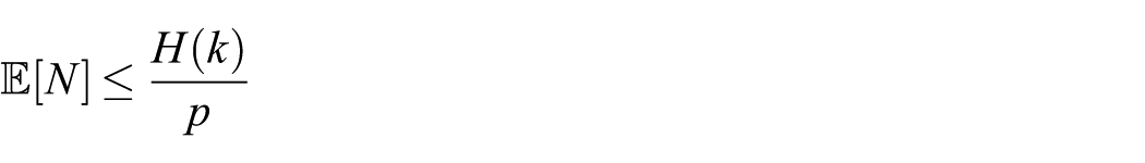
where
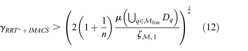
Following from analysis presented in Ladd and Kavraki (2004) and Proposition 3, it is easy to see that a random walk from
For the projection-based space, it is not known a priori what the volume is of an open neighborhood
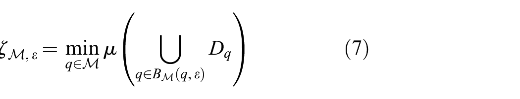
That is, for any
Proof. Let
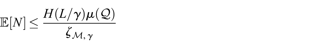
For the atlas-based space, we use theory developed in Jaillet and Porta (2012). Importantly, the following bound is presented for two points

where
where
Proof. As before, let
5.3.2. Discussion
Although here we present a proof of probabilistic completeness for PRM, the core of the proof applies to proofs for many other planners. This is because sampling, local planning, and metrics all behave nicely over
We briefly illustrate how the building blocks of sampling and local planning can be applied to other proofs of completeness. Similar to the proofs presented here, Kleinbort et al. (2019) presented a proof of probabilistic completeness of RRT. Without going into the details, the proof of probabilistic completeness of geometric RRT hinges on Lemma 1, which states that a local plan from a nearby random sample to its nearest neighbor lies entirely in
5.4. Asymptotic optimality
Asymptotically optimal sampling-based planners not only find a feasible solution, but as the number of iterations of the planner go to infinity, find the globally optimal solution. The algorithms RRT* and PRM* (Karaman and Frazzoli, 2011) are of particular interest, as they are the basis for many other asymptotically optimal algorithms and good case studies for how IMACS affects the necessary properties of an asymptotically optimal planner. Within this work, we describe how IMACS affects the proofs of asymptotic optimality for RRT* and PRM*; the features relevant that are affected by IMACS are the sampler, metric, and local planner. We walk through the affected portions of the proofs presented in Karaman and Frazzoli (2011) and show that their results hold given our assumptions about the metric and local planner within IMACS.
5.4.1. Prior results
Karaman and Frazzoli (2011) proved the following bound as the connection radius of RRT*:
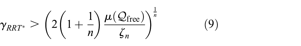
where
With respect to manifold constrained motion planning, Jaillet and Porta (2012) presented AtlasRRT*, an asymptotically optimal constrained sampling-based algorithm. AtlasRRT* adapts the RRT* algorithm with a continuation-based method for local planning and sampling. The following bound is given for the critical radius of AtlasRRT*:
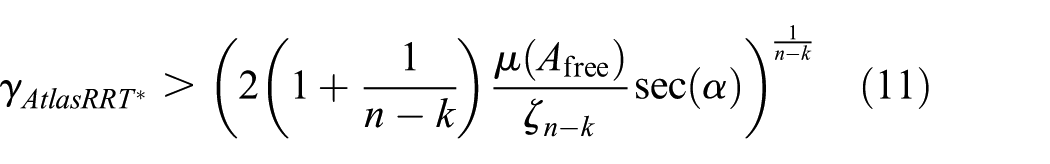
where
In terms of the measure on the atlas,
5.4.2. RRT* within IMACS
As mentioned in Jaillet and Porta (2012), the asymptotic optimality of RRT* is dependent on the ability of the planner to sample and connect configurations that are close to the optimal path. Importantly, the proof of RRT* is not dependent on the local planner being able to connect any two configurations. In fact, within Karaman and Frazzoli (2011), the proof of RRT*’s asymptotic optimality only relies on the local planner’s steering parameter
For the projection-based space, the connection radius is affected by the measure of set of states that project onto the free parts of the manifold, as samples are drawn from
Moreover, (11) can be applied to RRT* within the continuation-based space within IMACS, as the fundamentals of sampling and local planning are equivalent to those within AtlasRRT*.
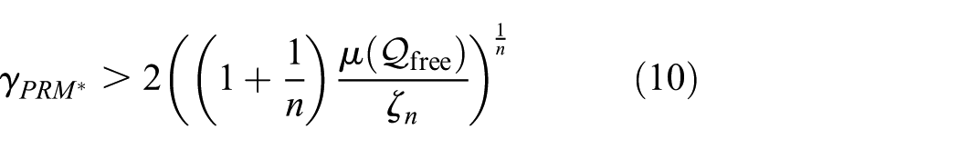
5.4.3. PRM* within IMACS
Critically for PRM*, IMACS affects the ability of a planner to connect subsequent vertices along the optimal path, as local planning within IMACS is only guaranteed for a neighborhood around a configuration. This is captured in the proof of PRM*’s asymptotic optimality (Karaman and Frazzoli, 2011) as an arbitrary constant
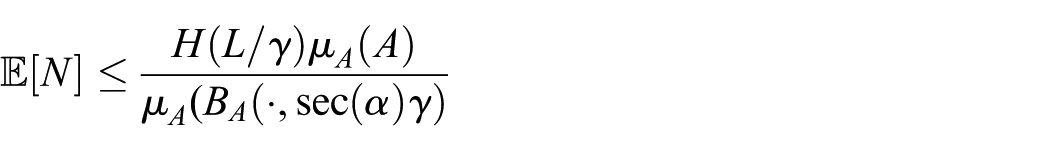
A bound similar to RRT* is claimed for PRM* in the projection-based space in IMACS:
Again, the critical features of sampling points are affected by the projection-based sampling method as well as the use of the ambient metric. Thus, the volume of
Observe that the bound is again in terms of measure on the atlas (giving the distortion constant
6. Experimental results
IMACS is implemented within OMPL (Şucan et al., 2012), an abstract library with implementations of many popular sampling-based planning algorithms. IMACS fits neatly within OMPL’s notion of a state space, and is implemented as such. In particular, IMACS is implemented as a state space that takes as input the ambient configuration space (also a state space) and a constraint function. Each of IMACS’s state spaces use the underlying subroutines offered by the ambient state space in tandem with their method of constraint adherence. No modification was necessary to any of the planning algorithms for them to work with IMACS. All of the code for the framework is available within OMPL, along with code to reproduce the most of the results presented in this section. 1
All benchmarks were done with a single set of parameters for each constrained space and planning algorithm, to preserve fairness across multiple environments. More performance could have been gained by tuning these for each problem, but a set of reasonable defaults is desirable, especially from a naıäve user’s perspective. All benchmarks were performed on workstations with an Intel® Core™ i7-6700K processor and 32 GB of DDR4 RAM at 2,400 MHz. The experiments shown here are meant to both demonstrate the effectiveness of the planning system as well as illustrate concepts that help put the work into context.
Within the presented results, we refer to three methods of constraint adherence running in IMACS: projection-, tangent bundle-, and atlas-based spaces. The projection-based space is as described in Section 4.2. The tangent bundle-based space is as described in Section 4.3 and uses the L
A critical aspect of constrained planning is the computation of the Jacobian of the constraint function as well as computing solutions to the (pseudo)inverse of the Jacobian. In general, analytic solutions to the Jacobian are preferable for efficiency. However, within our experiments, a few problems use numerical differentiation to compute the Jacobian when an analytical solution is not provided. Within our implementation of IMACS, the singular value decomposition (SVD) decomposition is used in the implementation of the projection operator (Algorithm 2), and the QR decomposition is used within
We performed a collection of experiments that demonstrate the important contribution IMACS represents: different planners and different methods of constraint adherence are better at different problems, IMACS is efficient and can be used for realistic problems, and planners within IMACS have similar performance to specialized constrained planners. The experiments include simple point robots in
6.1. “Sphere” environment
Figure 6 shows the “sphere” environment, a two-dimensional manifold embedded within
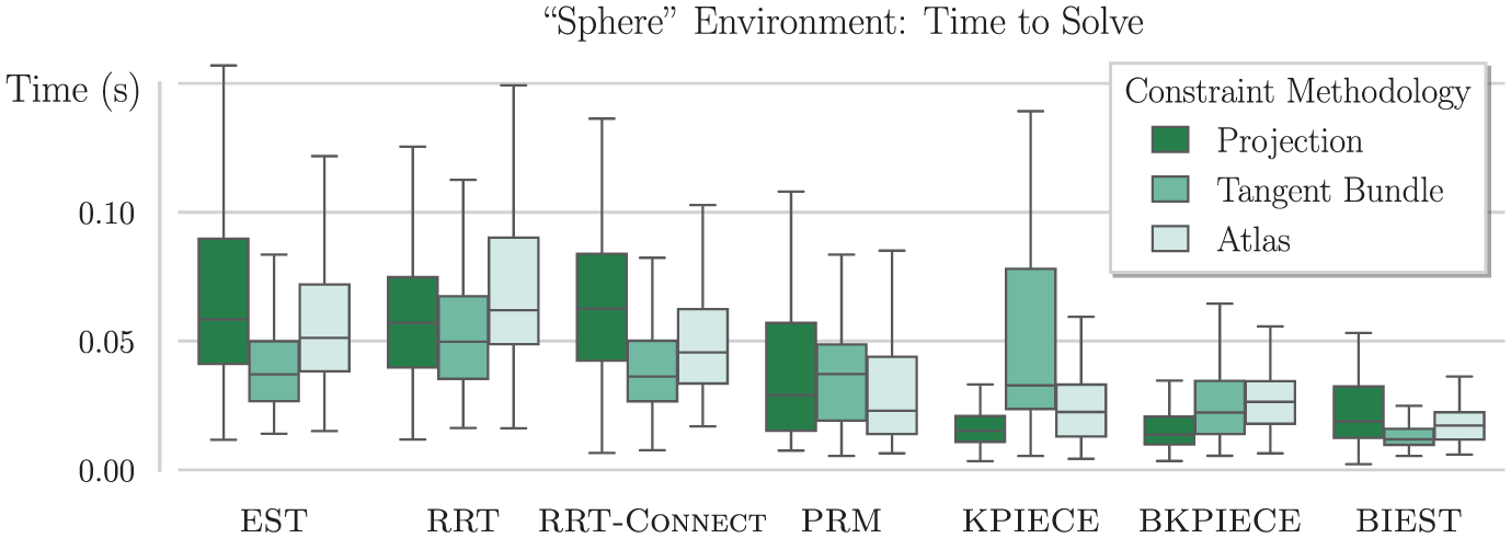
Timing results from 100 runs of each planner in the “sphere” environment (Figure 6) for the projection-, tangent bundle-, and atlas-based spaces in IMACS. Planners tested are EST, KPIECE, their bidirectional variants BIEST and BKPIECE (Hsu et al., 1999; Şucan and Kavraki, 2008), RRT (LaValle and Kuffner, 2001) and RRT-Connect (Kuffner and LaValle, 2000), and PRM (Kavraki et al., 1996). CBiRRT2, TB-RRT, and AtlasRRT are emulated by RRT-Connect in their respective constrained space, and have relatively poor performance.
There is little work on optimizing with respect to some cost function in tandem with manifold constraints. AtlasRRT* (Jaillet and Porta, 2013a) is an asymptotically optimal algorithm that adheres to manifold constraints, but requires specialized implementation and integration with a method of constraint adherence. Within IMACS, no additional overhead is necessary for asymptotically optimal planning, as shown in Figure 6, which shows motion graphs for three asymptotically optimal and near-optimal planners. In addition, path smoothing, shortening, hybridization, and interpolation algorithms work with no knowledge of constraints, as all subroutines are handled within IMACS. As proven in Section 5.4, asymptotically optimal planners retain their guarantees within IMACS.
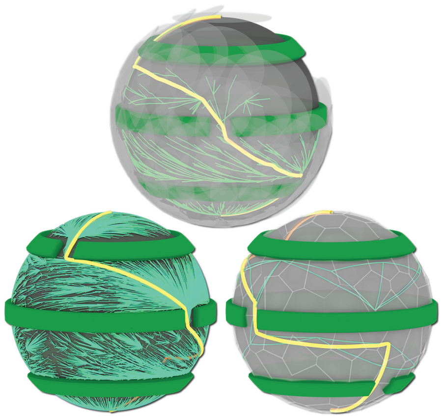
The “sphere” environment, from three perspectives. The sphere constraint manifold (gray) with obstacles (dark green). The solution path (yellow) runs from the south to north pole. From left to right, projection-based RRT* (Karaman and Frazzoli, 2011) motion graph (green), tangent bundle-based BIT* (Gammell et al., 2015) motion graph and tangent spaces (gray), and atlas-based SPARS (Dobson and Bekris, 2014) motion graph and tangent polytopes.
6.2. “Torus” environment
In constrained planning problems, not just the planner matters when solving a constrained problem; the ambient configuration space can dramatically affect performance. Consider a “torus” environment (Figure 7), which is a two-dimensional manifold embedded within

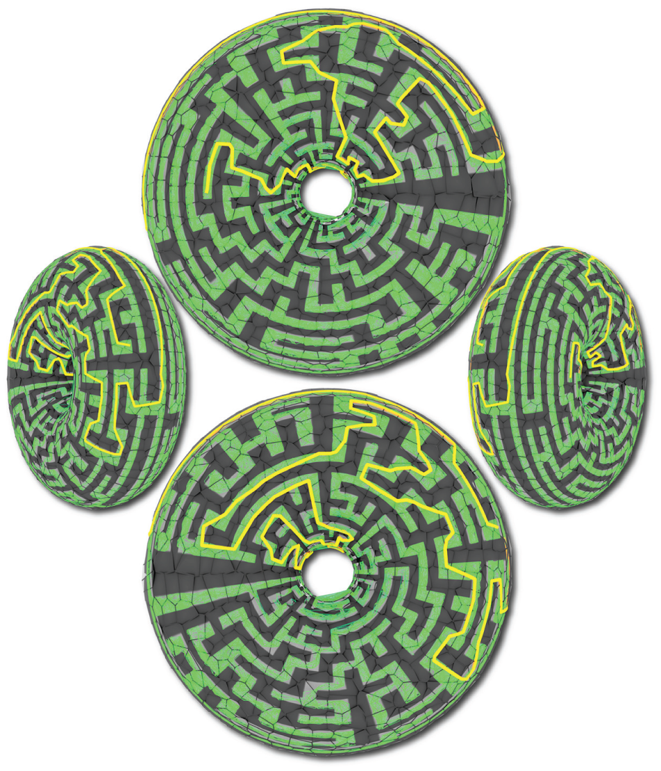
The “torus” environment. The torus constraint manifold (gray) with an overlaid obstacle maze and atlas. The resulting graph (green) of a run of atlas-based PRM along with a solution path (yellow) is shown on the torus.
For this environment, the robot is a point robot. The planning problem is to traverse a maze that is wrapped onto the surface of the torus. Timing results for the PRM planner using the projection- and atlas-based methods are shown in Figure 8, where the total volume of the configuration space is varied while the size of the torus remains constant. The volume of the configuration space is varied by increasing the bound b on the X- and Y-axes of the ambient configuration space (given by
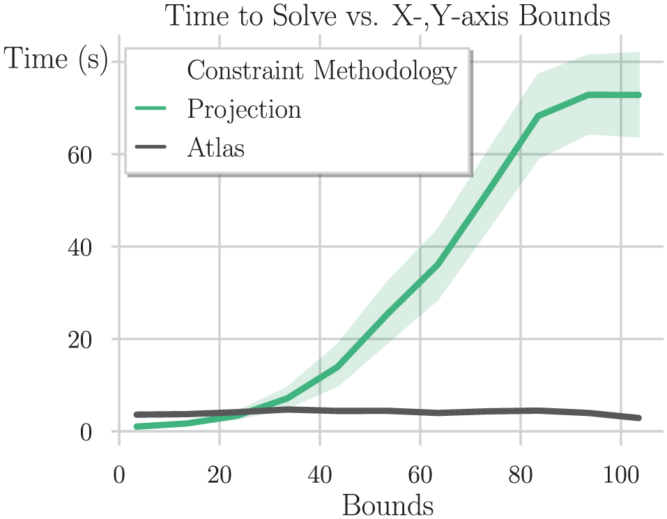
Timing results from 100 runs of PRM in the “torus” environment (Figure 2) using the atlas- and projection-based constrained space versus the size of the X- and Y-axes of the ambient configuration space. Projection-based PRM performs orders of magnitude worse than its atlas-based counterpart if the ambient space has a large volume, but is better when the ambient space is a tight bounding box.
As shown by the results in Figure 8, projection-based planning performs orders of magnitude worse than its atlas-based counterpart and worsens as the volume of the space expands, owing to the inefficiency of sampling configurations that mostly project to the outer surface of the torus. The atlas-based method, which samples directly from an approximation of the manifold, is unaffected by changes in the ambient configuration space. Projection to the inner surface of the torus requires sampling inside of the hole of the torus, which becomes less likely as ambient space expands. The torus example is illustrative of a problem that might arise on real robotic manipulators, as configuration spaces with revolute joints are toroidal in topology. It is unknown a priori how obstacles in the environment will interact with constraints, and no one method of constraint adherence is equipped to handle every case. Therefore, the ability to change method of constraint adherence independently of a planner is essential to efficiently planning within different environments.
6.3. “Implicit chain” environment
A general trend observed by the authors is that as a planning problem becomes more constrained or the implicit manifold more curved with respect to the ambient space, the atlas- and tangent bundle-based methods become more effective. This is because the extra computation to maintain the approximation pays off. However, as the dimensionality of the problem grows, the approximation is less helpful and requires a similar, amortized amount of work as projection does. These are not rules written in stone, and there are many problems that belie their guidance. Take, for example, the problem of an “implicit chain,” shown in Figure 9. Here, the kinematics are modeled as distance constraints, one for each link, on a chain with five spherical joints. The ambient configuration space is thus
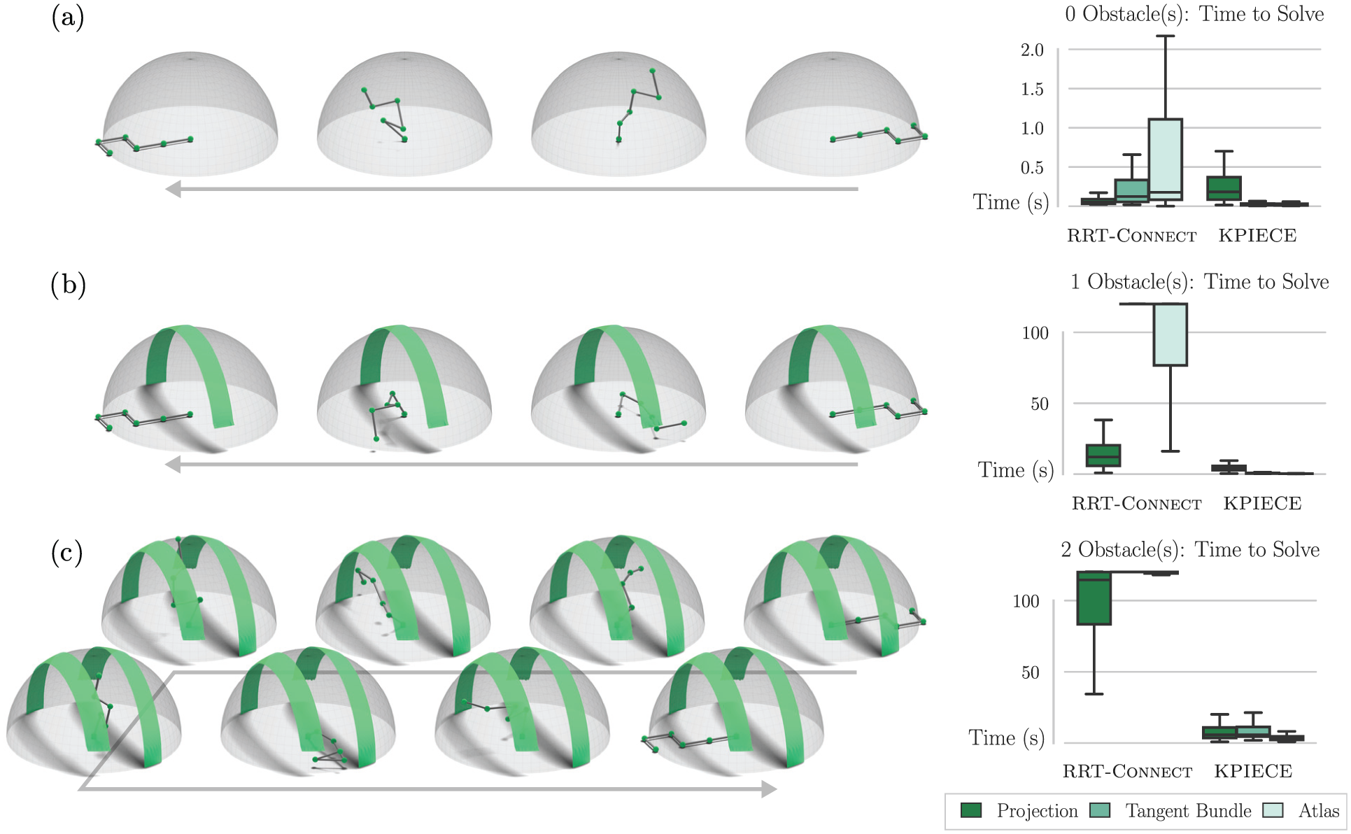
The “implicit chain” environment. Sample solution paths with zero (a), one (b), and two surface obstacles (c) with antipodal narrow passages are shown. In addition, timing results for RRT-Connect and KPIECE using each constrained space for each obstacle amount are shown on the right. A total of 100 runs were used for each combination of planner and constrained space, with a timeout of 120 seconds. Note that the Y -axis changes on the plots.
6.4. “Parallel implicit chain” environment
One motivating factor of this work was extending constrained planning to high-dimensional spaces, taking advantage of previous approaches in high-dimensional planning without any additional cost. In Figure 10, we show the “implicit parallel manipulator” environment, a parallel manipulator defined with a set of the “implicit chains” previously. The end-effectors of the chains are constrained to remain attached to a shared disk, creating dependencies in their motion. The environment shown has eight chains with seven links each, for a total ambient space dimensionality of 168. The constraint manifold is of dimension 99.
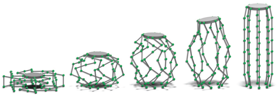
An plan in the “implicit parallel manipulator” environment. The goal is to move from a at, rotated configuration to upright. This path was computed using KPIECE in a projection-based constrained space in a median time of 14.5 seconds.
Recall that emulated prior works (CBiRRT2, TB-RRT, AtlasRRT) all use RRT-Connect as their base planner. RRT-Connect with in the projection-, tangent bundle-, and atlas-based spaces was unable to successfully solve this system given 10 minutes of planning time over 100 trials for each space. Using the KPIECE planner designed for high-dimensional spaces with the projection-based space, we can quickly solve this problem while adhering to constraints, for a median time of 14.5 seconds over 100 runs. As IMACS decouples the choice of planner and method for constraint adherence, IMACS enables more effective planners to be used for complex high-dimensional planning problems such as this.
6.5. Robonaut 2
Finally, we demonstrate the framework on a real robotic system. Figure 11 shows steps through a sequence of constrained motion plans for NASA’s Robonaut 2 (R2) (Diftler et al., 2011); R2 is tasked with walking through a narrow module on the International Space Station (ISS), with a few pieces of fixed, stray debris within. R2 is an excellent application for constrained motion planning due to the microgravity environment of the ISS, which allows for R2 to climb across handrails without typical humanoid worries such as dynamic stability. R2 maintains the quasistatic assumption throughout all motions.
Stills from a sequence of motion plans executed by NASA’s Robonaut 2 (R2) within a model of the ISS (sides of the module are removed for visualization purposes). R2 is modeled as a 15-DOF system with two 7-DOF legs and a rotating waist joint. In addition, an SE(3) element is added so the robot can float freely through the space. There are six separate motion planning problems in the sequence, each consisting of R2 taking a step. Each step with a variety of constraints imposed: (1) all steps required the torso to remain at a fixed orientation; (2) all steps fixed the position and orientation of the foot grasped to a handrail; and (3) where possible, the moving foot was required to face downward at a fixed orientation (a realistic requirement so the cameras within the feet can track handrail location).
In the above scenario, R2 is modeled as a 15-DOF system with two 7-DOF legs and a rotating waist joint. In addition, R2 has a floating joint (free-flying motion in
R2 must keep its torso upright at a fixed orientation;
one leg end-effector must remain fixed in position and orientation where it has grasped a handrail; and
whenever stepping towards an end-effector goal with the same orientation as the start, the moving foot must remain facing the same fixed orientation, so cameras within the end-effector can more accurately track handrail location for grasping.
An implementation of CBiRRT2 was compared against RRT-Connect running in the projection-based IMACS space, using the MoveIt! motion planning framework (Şucan and Chitta, 2011). Throughout the six motions, comparable timing performance was witnessed across 20 runs of each planner, with average planning times less than 5 seconds for both planners.
Functionally, the implementations of CBiRRT2 and RRT-Connect with the projection-based space in IMACS are nearly identical, with minor differences in how new states are generated via interpolation. Thus, the comparable performance of the planners is expected, and shows that in realistic scenarios there is no performance degradation using IMACS and an unconstrained planner.
7. Conclusion
We have introduced IMACS, a novel framework for sampling-based planning under manifold constraints that decouples constraint adherence from motion planning algorithms. With IMACS, the choice of motion planner and method for constraint adherence are orthogonal, enabling novel combinations of planner and method of constraint adherence that perform more effectively than previously proposed combinations. We have demonstrated IMACS’s capability by showing projection- and continuation-based methods of constraint adherence inspired by three state-of-the-art constrained sampling-based planners, CBiRRT2, TB-RRT, and AtlasRRT. In addition, we have tested a broad range of sampling-based planners within IMACS for a set of constrained problems and shown that each planner can operate effectively within IMACS. Furthermore, we have provided theoretical guarantees that IMACS preserves the probabilistic completeness and asymptotic optimality of planners running within IMACS. IMACS is easily extended to new planners, and new constraint spaces can be adapted to the framework as its concepts are general to constrained planning (e.g., local tangent space methods).
Although there are rough guidelines on when different constrained planning approaches tend to work better than others, for specific problems it is difficult to predict which combination of constraint space and planner will work the best. This further highlights the benefit of decoupling constraints from planning. In addition, the methods as presented here are dependent on some hyperparameters, such as the manifold integrator step size and chart validity parameters. Automatically tuning or adapting these parameters online while maintaining guarantees is left for future work.
Planning under manifold constraints is an essential capability for manipulation planning, task and motion planning, and multi-modal planing. Sampling-based planning with IMACS could be used as a subroutine for planning under constraints for these manipulation algorithms. The idea of IMACS is also extendable to the case of kinodynamic planning under manifold constraints. Finally, given the proof of concept on R2, we are in the process of integrating the framework for general robotic platforms.
Footnotes
Acknowledgements
We would like to thank the anonymous reviewers, Andrew Wells, and William Cannon Lewis III for their helpful comments, Caleb Voss for his preliminary work (Voss et al., 2017), and Dr. Julia Badger and the Robonaut 2 team.
Funding
The author(s) disclosed receipt of the following financial support for the research, authorship, and/or publication of this article: ZK, MM, and LEK are supported in part by the NSF (grant number IIS 1317849) and Rice University funds. ZK is also supported by a NASA Space Technology Research Fellowship (grant number 80NSSC17K0163).