Vision and Wi-Fi fusion in probabilistic appearance-based localization

Abstract

This article introduces an indoor topological localization algorithm that uses vision and Wi-Fi signals. Its main contribution is a novel way of merging data from these sensors. The designed system does not require knowledge of the building plan or the positions of the Wi-Fi access points. By making the Wi-Fi signature suited to the FABMAP algorithm, this work develops an early fusion framework that solves global localization and kidnapped robot problems. The resulting algorithm has been tested and compared with FABMAP visual localization, over data acquired by a Pepper robot in three different environments: an office building, a middle school, and a private apartment. Numerous runs of different robots have been realized over several months for a total covered distance of 6.4 km. Constraints were applied during acquisitions to make the experiments fitted to real use cases of Pepper robots. Without any tuning, our early fusion framework outperforms visual localization in all testing situations and with a significant margin in environments where vision faces problems such as moving objects or perceptual aliasing. In such conditions, 90.6% of estimated localizations are less than 5 m away from ground truth with our early fusion framework compared with 77.6% with visual localization. Furthermore, compared with other classical fusion strategies, the early fusion framework produces the best localization results because in all tested situations, it improves visual localization results without damaging them where Wi-Fi signals carry little information.

Keywords

Topological localization kidnapped robot low-cost sensors visual appearance Wi-Fi fingerprints data fusion

1. Introduction

1.1. Problem statement

This article addresses the problem of indoor localization for mobile service robotics. The current market trend consists of a mass deployment of affordable mobile robots interacting with humans. This raises the need for low-cost solutions enabling those robots to map their environment, and constantly know where they are when they move in it. Numerous projects have been proposed to solve the problem of localization. However, most of these solutions are based on the use of expensive sensors, such as laser range finders, and are designed for specific platforms (Kummerle et al., 2009).

The need for low-cost localization solutions has focused some research on the use of visual sensors. One investigation field aims attention at solving the problem of place recognition by using visual appearance (Angeli et al., 2008; Lowry et al., 2014; Lynen et al., 2014; Sünderhauf and Protzel, 2011; Ulrich and Nourbakhsh, 2000). Such algorithms try to associate query images to already mapped places, represented by their visual appearance. Lowry et al. (2016) presented a comprehensive survey of appearance-based approaches.

Our work is built upon the Fast Appearance-Based Mapping algorithm (FABMAP), introduced by Cummins and Newman (2008), that uses visual appearance to detect loop closures. This algorithm achieves robust localization with a low rate of false loop-closure detection and can manage big maps by employing an inverted index (Cummins and Newman, 2011).

However, place recognition algorithms using visual appearance have to face the well-known problem of perceptual aliasing. Perceptual aliasing happens when two different locations share similar visual appearances (see the example in Figure 1). This problem is inherent in repetitive environments. A solution is the use of multi-sensor localization for disambiguating such situations.

Fig. 1.

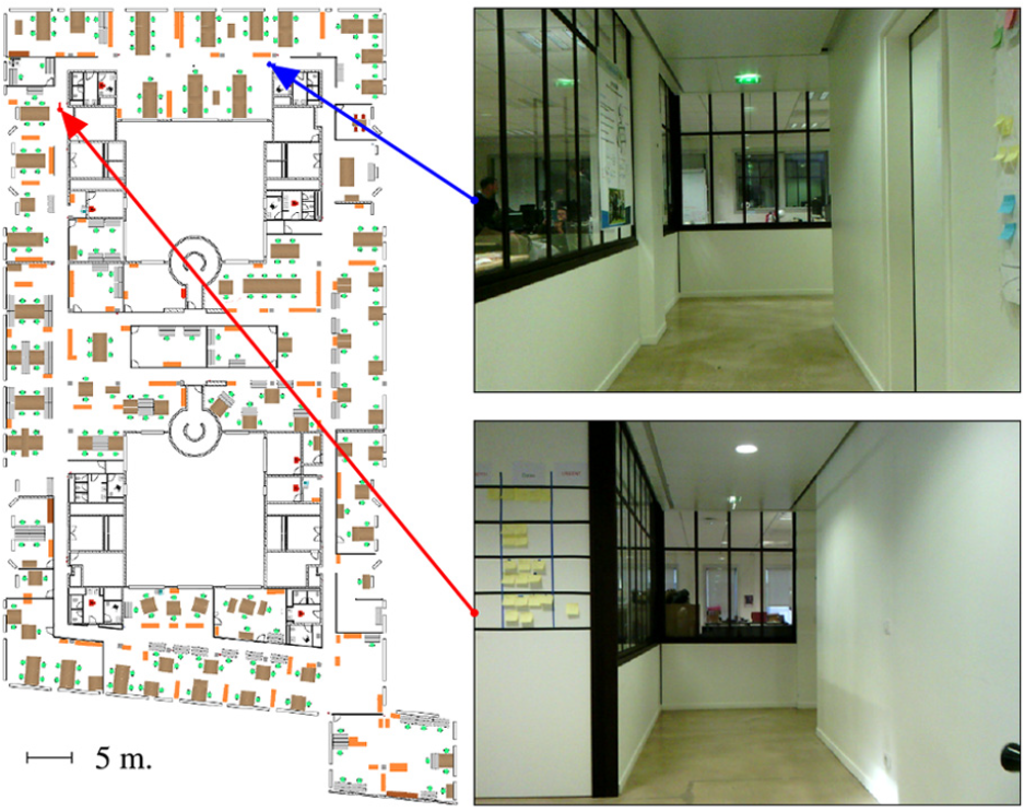
Perceptual aliasing. Two distant locations in a building share similar visual appearances. However, the perceived Wi-Fi signatures in these locations are different enough to distinguish between them.

Using Wi-Fi helps to disambiguate cases where several locations have similar visual appearances. For example, corridors on opposite sides of a building, or at different floors, have different Wi-Fi signatures but can share comparable appearances. Recent work has introduced a way of including Wi-Fi data into the FABMAP algorithm (Wietrzykowski et al., 2017), but it does not benefit from the advantages of both sensors since it only considers Wi-Fi signals.

In this article, a novel way of merging visual and Wi-Fi data is introduced in order to solve the global localization and the kidnapped robot problems.

1.2. Use case and social robots

Our novel merging scheme has been tested on Pepper robots, see Figure 2. Pepper is a social robot designed by SoftBank Robotics. It can be found mainly in Japanese shops, where it holds receptionist or demonstrator functions. One of Pepper’s key strengths directly comes from the interaction it has with users. These interactions are reinforced and simplified thanks to the human behaviors of the robot. For this reason, practical uses of Pepper result in special constraints taken into consideration in this work.

Fig. 2.

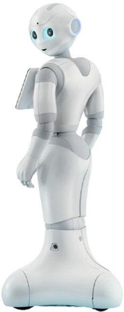
Pepper robot: designed for interacting with human beings as naturally and intuitively as possible. It was first presented by Lafaye et al. (2014).

First, the localization process must not hinder human–robot interaction. As such, it cannot take control of the joints of the robot, for example to make the robot look away from the human it is interacting with. Second, some Pepper robots are deployed in environments with little or no internet access. This implies that the localization function must be able to run, at a reasonable framerate, with the (limited) robot computing power.

A challenging use case comes from the initialization of the robot pose in its environment. When a Pepper robot is switched on to start its work day, it has to immediately localize itself without any help. This known problem is commonly called the global localization problem. It happens when the robot has no information about its previous pose. A very similar issue is often referred to as the kidnapped robot problem. This problem corresponds to situations where the robot has a false prior on its pose. Both problems are very similar, and methods solving global localization problem can be adapted to solve the kidnapped robot problem. Our work aims at solving these problems in indoor situations that are typically the operation environments of Pepper robots.

1.3. Related work

In recent years, several indoor localization algorithms based on Wi-Fi sensors have been introduced (Biswas and Veloso, 2010; Boonsriwai and Apavatjrut, 2013; Howard et al., 2003; Huang et al., 2011; Jirku et al., 2016; Olivera et al., 2006; Rohrig and Kiinemund, 2007). This popularity can be explained by two factors. First, the Wi-Fi coverage in urban environments is dense enough for use in localization tasks. Second, it is easy to equip mobile robots with Wi-Fi sensors.

Because the Wi-Fi localization error is bounded (Olivera et al., 2006), some algorithms choose to fuse Wi-Fi with other sensors (Aparicio et al., 2008; Mirowski et al., 2013; Ocaña et al., 2005). Visual and Wi-Fi localizations are particularly complementary. Even if Wi-Fi localization is less accurate (Liu et al., 2012), it does not suffer from perceptual aliasing, visually dynamic or repetitive environments. A lot of strategies take advantage of this synergy and use visual and Wi-Fi sensors to create a low-cost localization.

Most work focusing on solving the localization problem from these sensors uses particle filters for fusion as in Schwiegelshohn et al. (2013), Quigley et al. (2010), and Liu et al. (2017). However, the hypothesis converges if there is enough motion. Other approaches are sequential, and usually Wi-Fi guided. They define a set of possible locations from Wi-Fi data, and perform visual localization over it (Jiang and Yin, 2015; Nowicki, 2014; Ruiz-Ruiz et al., 2011; Werner et al., 2011). Finally, some methods consist of choosing which sensor is the most reliable for current estimation (Biswas and Veloso, 2013). Yet, these two last approaches are both likely to suffer from one misled sensor.

1.4. Contribution

Our main contribution is a novel way of merging Wi-Fi and vision for localization tasks. We propose an early fusion process for combining visual and Wi-Fi data that takes the same inputs as the classical FABMAP. In comparison with related work, our approach looks for a compromise on the current estimation by considering data from both sensors together.

The core of our algorithm was first presented in Nowakowski et al. (2017). In this article, our method considers the Wi-Fi signal more deeply. Experiments from Nowakowski et al. (2017) are augmented with new data making the results presented in this article more precise and reliable. New tests are specifically realized in multiple environments to evaluate the generality of our solution.

1.5. Paper organization

To introduce our localization solution using Wi-Fi and vision, the FABMAP algorithm is first briefly presented in Section 2. The readers familiar with FABMAP can start with Section 3 that explains how Wi-Fi data is made compatible with the FABMAP formalism. Our early fusion process is then introduced in Section 4 with other merging strategies for comparison. Finally, our experimental acquisitions and localization results are presented and discussed in Section 5.

2. Fast appearance-based mapping

Cummins and Newman (2008, 2011) introduced FABMAP, for fast appearance-based mapping, a localization algorithm based on the visual appearance. FABMAP discretizes the environment into a succession of topological nodes. Each node constitutes a location $L_{i}$ , and is associated with one or several visual observations. When processing a query image, FABMAP uses the results of an offline learning stage. This learning is achieved before the map creation and the localization phase over external data.

Given a query image, the goal of FABMAP is to compute the following value for each place $L_{i}$ in a topological map:

p (L_{i} | Z^{k}) = \frac{p (Z_{k} | L_{i}, Z^{k - 1}) p (L_{i} | Z^{k - 1})}{p (Z_{k} | Z^{k - 1})}

(1)

where $Z_{i}$ is the ith observation and $Z^{i}$ is the set of all observations, up to i. Three terms can be identified in (1): the likelihood $p (Z_{k} | L_{i}, Z^{k - 1})$ , the normalization term $p (Z_{k} | Z^{k - 1})$ , and $p (L_{i} | Z^{k - 1})$ that can be considered as a prior knowledge on the current pose because the approach assumes independence between current pose and past observations. Note that in our work, this last term is not used because our intention is to solve the global localization problem.

The three next subsections introduce the computations of the observation $Z_{k}$ , the likelihood, and the normalization term, respectively.

2.1. Visual appearance description

The first step of FABMAP is to transform a query image into a compact image descriptor that is suited to the localization context. This compact descriptor is called the observation vector, or visual appearance, and is denoted by Z in (1). To do this, FABMAP uses the bag-of-words approach introduced in computer vision by Sivic and Zisserman (2003). Keypoints are extracted in the image, and their descriptors are then associated with words of a vocabulary. In FABMAP, the observation Z indicates which words of the vocabulary are present on the query image.

For a vocabulary of N words, Z thus contains N binary values indicating the presence or absence of the corresponding word in the query.

The vocabulary used comes from offline learning. It is usually built thanks to a clustering method such as the k-means performed over a lot of keypoints descriptors extracted from learning images. Learning images can be chosen in databases according to the operating environment of the algorithm (indoor, outdoor, etc.).

2.2. Observation likelihood

The second step constitutes the core of the algorithm and computes the likelihood term $p (Z_{k} | L_{i}, Z^{k - 1})$ conditioned on the location. This term is simplified into $p (Z_{k} | L_{i})$ in Cummins and Newman (2008), assuming independence between the current pose and past observations. Approaches using the bag-of-words framework can compute similarity scores between queries and references thanks to methods such as the Term Frequency - Inverse Document Frequency (Salton and Buckley, 1988), or hierarchical vocabularies (Nister and Stewenius, 2006). The main contribution of FABMAP is the use of a Chow Liu tree (Chow and Liu, 1968), that captures correlations between the different words of the vocabulary. This approach is motivated by the fact that certain visual words are often detected on specific objects and, thus, tend to co-occur. In general, these correlations are learnt offline, with the database used during the vocabulary creation.

Experiences realized in Cummins and Newman (2008) show that learning these correlations helps to avoid false associations owing to perceptual aliasing. It also helps to achieve correct associations between images, even if they share few words in common.

2.3. Normalization

The normalization step allows the detection of unknown locations. Cummins and Newman (2008) split $p (Z_{k} | Z^{k - 1})$ into two sums, one representing the visited locations M, the other the unknown world $\bar{M}$ :

\begin{matrix} p (Z_{k} | Z^{k - 1}) = \sum_{m \in M} p (Z_{k} | L_{m}) p (L_{m} | Z^{k - 1}) \\ + \sum_{u \in \bar{M}} p (Z_{k} | L_{u}) p (L_{u} | Z^{k - 1}) \end{matrix}

(2)

The second summation cannot be evaluated directly. The authors of FABMAP propose to approximate (2) by

\begin{matrix} p (Z_{k} | Z^{k - 1}) \approx \sum_{m \in M} p (Z_{k} | L_{m}) p (L_{m} | Z^{k - 1}) \\ + p (L_{new} | Z^{k - 1}) \sum_{u = 1}^{n_{s}} \frac{p (Z_{k} | L_{u})}{n_{s}} \end{matrix}

(3)

where $p (L_{new} | Z^{k - 1})$ corresponds to the probability of being in a new location, and is a user-specified input of the algorithm (set to 0.9 in Cummins and Newman (2008)). The second sum of (3) consists of sampling an observation Z to create a place model associated with unknown location. The sampling of Z is realized from a training set of $n_{s}$ images.

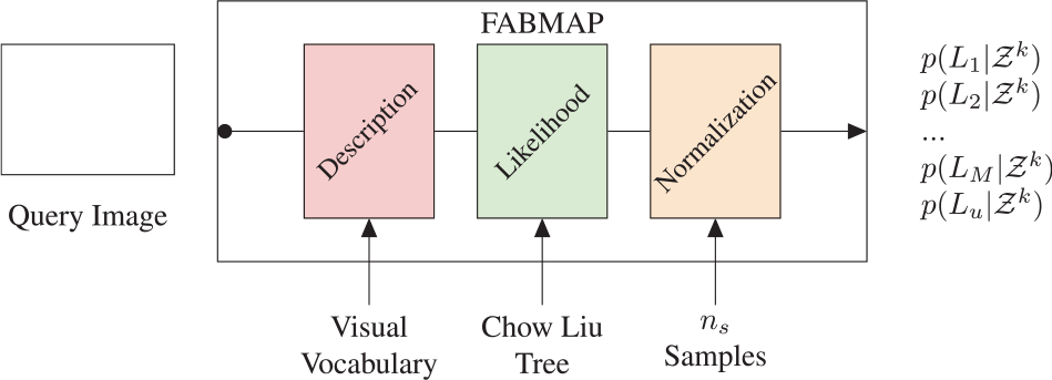
In addition to the vocabulary, the Chow Liu tree and the $n_{s}$ samples, the authors of Cummins and Newman (2008) list some user-specified inputs. In our work, these parameters are set to the values specified in Cummins and Newman (2008). Figure 3 summarizes the successive steps of the algorithm.

Fig. 3.

Inputs of each steps of the FABMAP algorithm.

3. Including Wi-Fi data in FABMAP

In the related literature (Biswas and Veloso, 2010; He and Chan, 2016; Liu et al., 2012), a Wi-Fi signature, sometimes referred to as a fingerprint, consists of a list of visible access points (APs), each one being characterized by its MAC address and its signal strength (received signal strength indication (RSSI)). Most of Wi-Fi localization algorithms collect Wi-Fi signatures during an exploration stage and then generate a map modeling the distribution of Wi-Fi signals in the environment. Such approaches have the advantage of not requiring knowledge of the positions of the APs in the environment. These strategies particularly suit the topological localization of FABMAP once they are made compatible with it (Nowakowski et al., 2017; Wietrzykowski et al., 2017). This section introduces how our work integrates Wi-Fi information into FABMAP, following the steps of Figure 3.

3.1. Defining a Wi-Fi vocabulary

The first step of visual FABMAP consists of turning a query image into a vector of binary values: the visual appearance. This vector is built thanks to a vocabulary of visual words. To do the same thing with Wi-Fi signatures, a correct definition of what is a Wi-Fi word is needed.

In previous work (Nowakowski et al., 2017), each MAC address characterizes one Wi-Fi word. In contrast with classical visual vocabulary, Wi-Fi vocabulary can therefore only be built online or after an exploration phase. Indeed, it is useless to define a global and complete Wi-Fi vocabulary since it is not possible to know the APs a robot is going to encounter in an environment before exploring it. After an exploration phase, the encountered MAC addresses constitute the vocabulary. The values of Wi-Fi observation vector $Z_{Wi - Fi}$ indicate which known APs are visible in a Wi-Fi signature. However, this definition does not take advantage of the information carried by the RSSI.

Wietrzykowski et al. (2017) discretized the Wi-Fi signal strength over 10 bits in the range $[- 110 dBm, - 10 dBm]$ . Each bit is associated with a threshold and is set to 1 if the perceived signal strength exceeds this threshold. Consequently, the Wi-Fi signal identified by a MAC address is described by 10 words in the observation vector.

That last method can be seen as an incremental representation. Even if such representation is expected to manage small temporal variations of RSSI, it is possible that the strongest correlations learnt between words of the vocabulary come from Wi-Fi words associated with the same APs. Our work thus introduces another technique that we call the exclusive representation. A signal coming from a MAC address is still described by multiple words, but only one word is set to 1 following its RSSI. A range for usable RSSI is defined and split into multiple b bins. Each bin is associated with one binary value. When the perceived signal strength is between the upper and lower limits of a bin, its value is set to one. Otherwise, it is set to zero. Thus, it is possible to compute a vector of b words for each perceived signal in a Wi-Fi signature. A comparison of the incremental and exclusive representations is shown in Figure 4 for a Wi-Fi signal identified by a MAC address and described by $b = 5$ Wi-Fi words.

Fig. 4.

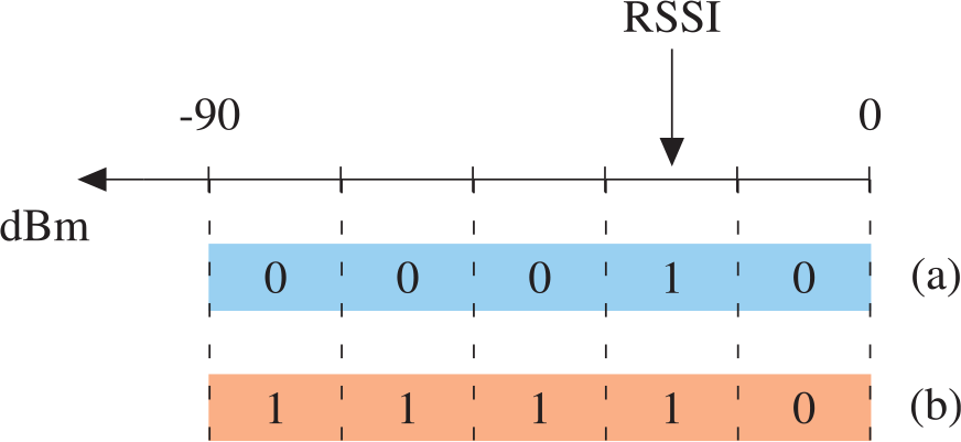
Example of Wi-Fi signal perceived from an AP being encoded over $b = 5$ words with the exclusive (a) and the incremental (b) methods.

With both approaches, $Z_{Wi - Fi}$ is the ordered concatenation of the vectors describing the signals of all known APs in the current signature. Each unperceived AP of the vocabulary in current signature is associated with a vector full of zeros. Thus, with $K_{W}$ known MAC addresses, a Wi-Fi signature is transformed into an observation vector $Z_{Wi - Fi}$ of $b \times K_{W}$ binary values.

At a given location, Wi-Fi signal strength varies significantly. To make their inputs more reliable, most Wi-Fi localization solutions stay motionless for a while, and compute mean and standard deviation of the RSSI coming from each AP (Biswas and Veloso, 2010; Jirku et al., 2016). This approach is not possible in our use case because of Pepper’s motion behaviors. Therefore, the issue of how many words to use for encoding Wi-Fi intensity arises without the possibility of averaging. If the use of a lot of Wi-Fi words is expected to increase the accuracy, a too precise representation can mislead our system. This issue is investigated in Section 5.8.

3.2. Tree structure

The previous subsection explained that Wi-Fi vocabulary can only be built and completed online or after an exploration phase. It is thus possible to build a Chow Liu tree that catches correlations between Wi-Fi words from the collected Wi-Fi signatures. However, in order to avoid the learning of redundant correlations, it is necessary to make sure that observation vectors come from different places. In our system, spatial difference is ensured thanks to odometry data and temporal difference is ensured by timestamps.

3.3. Normalization and virtual Wi-Fi locations

In the visual world, sampling an observation for normalization is easy. To do this, training images needed during the offline learning and coming from other environments are used. In the Wi-Fi world, employing this method is not so simple. One Wi-Fi vocabulary is specific to one environment. For this reason, using real Wi-Fi signatures collected in training environments does not make a lot of sense since the computed observation vectors would only be composed of zeros. A solution is to simulate virtual Wi-Fi signatures according to the collected data.

Multiple variations in Wi-Fi signatures can be identified for unknown locations considering the propagation of Wi-Fi signals. An unknown location can:

share the same Wi-Fi signature as a mapped place;

have unknown APs in its Wi-Fi signature;

bring up new combinations of known APs.

Virtual Wi-Fi signatures are simulated considering these changes.

In our measurements, the number of APs in a Wi-Fi signature follows a normal distribution for a specific environment. The mean $μ$ and the standard deviation $σ$ on the number of APs perceived in the Wi-Fi signatures collected during the exploration are thus identified. To randomly generate a virtual Wi-Fi signature, our method first selects a number of perceived APs following the normal distribution $N (μ, σ)$ . Each of these simulated APs is then randomly associated with a known or unknown MAC address and an RSSI in the usable range of strength defined (in our case $] - 90 dBm, 0 dBm]$ ).

With this formalism, FABMAP localization results based on Wi-Fi data can be computed. However, as shown in Section 5, using Wi-Fi data alone shows poorer accuracy than visual-based localization. Next section explains how to take advantage of both visual and Wi-Fi sensors.

4. Merging visual and Wi-Fi data

This section introduces various fusion strategies, and among them, our early fusion process. To the best of the authors’ knowledge, this approach has not been studied previously for solving the global localization problem using Wi-Fi and visual data. Our methodology is shown in Figure 5. The following subsections present more classical ways of merging vision and Wi-Fi, discuss the interest of the early fusion framework, and our choices concerning the inputs of this algorithm.

Fig. 5.

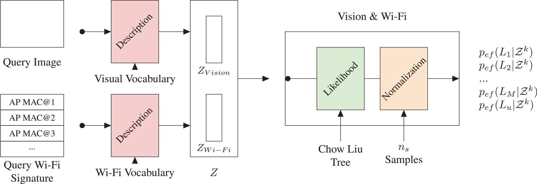
Early fusion framework, using visual and Wi-Fi data.

4.1. Sequential fusion

In multi-sensor systems, sequential fusions try to take advantage of the different levels of accuracy of the different sensors. Two methodologies can be identified when using sequential fusion with Wi-Fi and visual data:

Wi-Fi-guided fusion, in which a visual localization is realized over possible locations determined from Wi-Fi data;

Wi-Fi check fusion, where the result from visual localization must be confirmed by Wi-Fi data.

These approaches use the fact that Wi-Fi localization is less accurate than visual localization, but never produces aberrant results. However, FABMAP normalization style enables the algorithm to detect loop closures with the assumption that no one has been missed. In practice, FABMAP detects at most one loop closure for each query. However, in order to make the presented sequential fusions work, Wi-Fi localization has to furnish a set of several possible locations. Work presented by Stumm et al. (2013) tackles this issue by introducing another normalization approach. The same technique is used in our evaluated sequential merging strategies.

4.2. Late fusion and early fusion

An intuitive way of merging localization results coming from multiple sensors can be called late fusion. Each sensor s provides a probability $p_{s} (L_{i} | Z_{s}^{k})$ of being in a location $L_{i}$ knowing its observations $Z_{s}^{k}$ . For a multi-sensor platform composed of two sensors $s_{1}$ and $s_{2}$ , the result $p_{lf}$ from the late fusion can be written as

p_{lf} (L_{i} | Z_{s_{1}, s_{2}}^{k}) = α \times \frac{p_{s_{1}} (L_{i} | Z_{s_{1}}^{k}) p_{s_{2}} (L_{i} | Z_{s_{2}}^{k})}{p (L_{i})}

(4)

where $α$ ensures that $\sum_{i} p_{lf} (L_{i} | Z_{s_{1}, s_{2}}^{k}) = 1$ . Focusing on the global localization problem and considering that $n_{M}$ locations have been mapped, plus one location associated with the unknown world, note that for every i, $p (L_{i}) = \frac{1}{n_{M} + 1}$ .

With late fusion, each localizer gives a result according to the perceptual area of its sensor. Therefore, a sensor misled by perceptual aliasing can clearly pervert the system. In this work, we propose to merge the data before the steps of likelihood computation and normalization. We thus realize an early fusion framework. The output probabilities of the algorithm are denoted $p_{ef} (L_{i} | Z^{k})$ . The idea is to concatenate the observation vectors obtained from visual and Wi-Fi sensors as presented in Figure 5. This resulting observation vector then becomes the query for a single localization algorithm. The early fusion asset is the computation of a compromise between the different sensors.

The overall process of early fusion thus corresponds to the classical FABMAP using as input the concatenation of visual and Wi-Fi appearance vectors. Computing $p_{ef} (L_{i} | Z^{k})$ is done in the same way as described in Sections 2.2 and 2.3. The learning of correlations between vocabulary words driving the computation of likelihood and normalization terms is presented in the following subsection.

4.3. Which correlations to learn for early fusion?

When merging Wi-Fi and visual data by early fusion, the question of which correlations to learn remains. We choose to split the correlations learning. Instead of learning one tree, two trees capture words that co-occur in the visual vocabulary and in the Wi-Fi vocabulary, respectively. Both trees are passed together as a single data structure to the localization algorithm. This split learning can be explained by two reasons.

First, learning new correlations between all Wi-Fi and visual words is not obvious. For instance, to learn new visual correlations from nodes collected during exploration, all visual words of the vocabulary must have been seen at least once during the exploration. In practice, it is not possible to ensure that this assumption is verified.

Second, the normalization step encourages this choice. Indeed the visual and Wi-Fi unknown world is too difficult to simulate whereas using split learning allows to simply concatenate unknown visual and Wi-Fi samples.

Even if the correlations learning is split, Section 5 shows that early and late fusions generate different results. Both fusions are also compared with sequential fusions (Section 4.1) that are more classical Wi-Fi and vision merging styles.

5. Evaluation

5.1. Experimental conditions

Our algorithm was evaluated on data acquired by several Pepper robots. Each robot used was equipped with the same camera model and the same Wi-Fi device. In these conditions, the differences in localization performances were not significant from one robot to another. The use of several robots showed that localization results are robust to the small hardware differences that may exist between devices, such as camera calibration or Wi-Fi antenna characteristics. Each acquisition was done by driving a Pepper thanks to a remote control. During the acquisitions, the robot autonomously acquired images every 2 s, and Wi-Fi signatures every 10 s, while moving at an average speed of $0.35 m s^{- 1}$ . Diverse constraints came from the need for a visually natural localization (Section 1.2). For instance, blurry images could result from the fact that we did not want the robot to stop for image acquisitions. Moreover, motion behaviors of the robot were kept. When navigating, Pepper looks in the direction of its motion. Thus, in straight lines, images were not taken in discriminative perpendicular directions (left or right), but in the direction of movement. Extension 1 illustrates the data acquisition and localization process.

In order to see the performances of our system, multiple environments were used in this article. During our acquisitions, the environments were not specifically equipped and the tested localization algorithms only used the existing visual and Wi-Fi landmarks. Thus, data has been collected in:

the open spaces of an office building on two different floors (Section 5.4);

corridors and classrooms of a junior high school spread over three different floors (Section 5.5);

the different rooms of a private apartment (Section 5.6).

Each of these environments has some specific aspects. However, because Pepper is intended to be handled by non-expert users, the same acquisition scheme was kept in all these situations.

The paths we ran constitute a set of 10,120 images and 6,110 Wi-Fi signatures. The total covered distance is 6.4 km long. We also paid attention to the diversity and reality of our acquisition scenarios: occlusions, dynamic environment, realistic velocity, user interactions, blur, various times of day, etc.

Finally, the visual vocabulary used was learnt from 3,000 images of indoor scenes, extracted from database presented in Quattoni and Torralba (2009). To satisfy the real-time constraint, FAST keypoints detection was used (Rosten and Drummond, 2006; Rosten et al., 2010) combined with the ORB binary descriptors (Rublee et al., 2011).

5.2. Annotations: initial exploration and localization

Our formalism defines topological nodes by an associated couple (image ; Wi-Fi signature). In practice, images were collected faster than Wi-Fi signatures. Therefore, in order to associate acquired images with Wi-Fi signatures, two scenarios were chosen for mapping and localization phases, respectively:

during the initial exploration phase, images were associated with the estimated temporally closest Wi-Fi signature;

during the localization tests, images were linked to the last Wi-Fi signature acquired.

The positions of all collected images were manually annotated, resulting in ground truth of node positions. For each environment, the different acquisitions were split in two: 40% were used for map creation and 60% constituted our queries. Each query corresponded to a mapped place. Global localization was thus realized in an entirely mapped environment.

Note that all Wi-Fi correlations were learnt over examples used for the mapping.

5.3. Evaluation metrics

For each query, the highest score computed by the algorithm was considered as the current localization in the map:

L_{\max} = \underset{L_{i} \in M \cup \bar{M}}{argmax} p (L_{i} | Z^{k})

(5)

To evaluate accuracy, the Euclidean distance between the annotated positions $(x, y)$ of the query and the associated mapped place $L_{\max}$ was computed. This distance was set to infinity when the algorithm was mistaken between two floors or two environments. This choice is explained by the fact that these kind of errors are much more problematic in practical cases. Finally, when $L_{\max} = L_{u}$ , corresponding to unknown location, our evaluation considered the result as rejected.

The results are discussed in the following. We have used the FABMAP2.0 algorithm (Cummins and Newman, 2011), and adapted the open-source implementation introduced in Glover et al. (2012) to our use. For the set of queries, localizations were computed using visual data only, Wi-Fi data only, and different merging styles: early and late fusions, and the two sequential fusions presented in Section 4.1.

In order to appraise the global localization performances of the different merging approaches, results are presented according to two types of graphs showing:

the rate of correct localizations, measured as the cumulative distribution of distances between estimated localizations and ground truth;

the rate of misplaced localizations, measured as the percentage of queries leading to localizations farther away from ground truth than a given distance.

Thus, both types of graphs show different information. If the first gives information on the accuracy of the algorithms, the second highlights its errors. On graphs showing the rate of misplaced localizations, the different rejection rates can be deduced as

1 - Rate (error > d = 0)

(6)

Appearance-based SLAM algorithms are sometimes evaluated on a topological best-place correct rate. Because of the nature of Wi-Fi based localization, which is not as precise as visual localization, we chose to evaluate our algorithm on its metrical correctness. It also makes sense for the kidnapped robot problem to know how far, geometrically, the algorithm is from ground truth. If needed, the presented results can be interpreted as a topological best-places correct rate. Given the robot moving speed and data acquisition frequency, references are placed, on average, every 70 cm. As stated earlier, queries were made only on an already mapped route, which makes each query at most 35 cm away from its closest reference. Our main performance index is the rate of correct localizations within 5 m, which corresponds to a match with one of the 10 best topological places.

In the following subsections, localization results in various environments are presented. First, signal strengths in Wi-Fi signature will not be used. Only the presence or absence of known APs will be taken into account. The use of RSSI will then be specifically investigated in Section 5.8.

5.4. Localization in an office building

The environment where most of our acquisitions were realized is the office floors of SoftBank Robotics Europe that are mainly composed of open spaces. This facet is significant considering the propagation of Wi-Fi signals. In such environments, Wi-Fi signatures are more difficult to distinguish because there are no obstacles creating important changes. Possible uses of Pepper in large indoor environments, such as shops, malls, or airports, have motivated this choice of testing conditions.

Acquisitions were realized with different Pepper robots over several months and on two different floors of the building. Some examples of paths run by Pepper on a floor of the office building are shown in Figure 6.

Fig. 6.

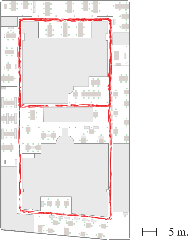
Examples of paths run by Pepper robots on a floor of SoftBank Robotics Europe office building.

5.4.1. Evaluation of early fusion

In such testing conditions, the use of Wi-Fi data was expected to decrease the number of aberrant localizations. Indeed, the particularly dynamic and repetitive aspects of the open space make the APs more stable landmarks than visual keypoints. These expectations were verified by the results plotted in Figure 7(a) and (b). The localization based only on Wi-Fi produced 1.3% of aberrant estimations localized more than 20 m away from ground truth whereas classical visual FABMAP generated 8.3% of deviant localizations. However, the visual localization still resulted in more accurate results with 75.0% of the queries localized within 2 m of their true positions.

Fig. 7.

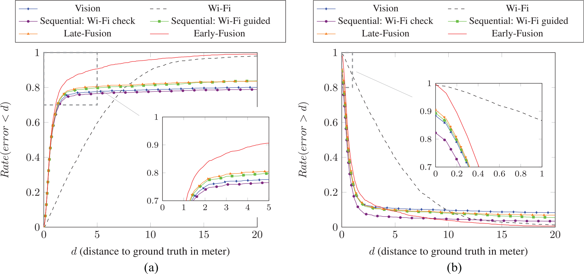
Localization results computed from the different localization algorithms in the office building of SoftBank Robotics Europe. (a) Rate of correct localizations. (b) Rate of misplaced localizations.

The interest of combining Wi-Fi and vision for localization tasks is confirmed by the results introduced in Figure 7(a) and (b). All presented merging approaches show rates of misplaced localizations lower than visual FABMAP for a distance of 5 m. Concerning the rates of correct localization, our early fusion framework clearly outperformed the other algorithms with 90.6% of the queries localized within 5 m of their true positions, compared with only 77.6% for vision only. In Figure 7(b), the rejection rate of sequential fusion with Wi-Fi check allowed us to reduce the rate of errors for this merging style, but the price to pay was high: in about one in five cases (17.8%, cf. the curve in Figure 7(b) at $d = 0$ ), the robot did not succeed in estimating a position.

Resulting values from early fusion and Wi-Fi check localizations are listed in Table 1 for comparison with classical FABMAP.

Table 1.

Comparison of classical FABMAP with the presented localization schemes using Wi-Fi data only, and merging visual and Wi-Fi data.

	Correct localization rate (%) within				Misplaced localization rate (%) away from
	2 m	5 m	10 m	20 m	2 m	5 m	10 m	20 m
Vision	75.0	77.6	78.7	80.1	13.4	10.8	9.7	8.3
Wi-Fi	26.0	59.7	89.8	98.0	73.3	39.6	9.5	1.3
Wi-Fi guided	76.5	79.7	81.3	83.8	12.8	9.6	8.0	5.5
Wi-Fi check	73.9	76.5	77.5	78.8	8.3	5.8	4.7	3.4
Late fusion	77.1	80.5	82.0	83.6	13.4	9.9	8.4	6.9
Early fusion	82.9	90.6	95.9	99.1	16.8	9.1	3.9	0.6

Examples of complicated query images taken in the environment are shown in Figure 8. The images chosen highlight some typical complex situations. This environment was particularly dynamic since all acquisitions were realized during office hours. Between two runs of the robots, furniture could be moved, people were not systematically sitting at the same place, and light conditions could evolve significantly. Furthermore, people were not asked to avoid interaction with Pepper. Most of acquisitions thus contained occlusions due to interactions or people walking in front of the camera (queries (a) and (b) in Figure 8). In all cases of images with occlusions, early fusion produced similar or better pose estimations than the visual localization. Queries (c) and (d) in Figure 8 indicate some examples of perceptual aliasing. Query (c) was misled by the presence of a houseplant that produced a lot of visual keypoints. A similar houseplant on another floor of the building duped the visual localization. The early fusion process did not reproduce this error thanks to the use of Wi-Fi data. A very difficult case of perceptual aliasing can be seen with query (d) of Figure 8. In this case too, the early fusion framework generated an acceptable localization (0.70 m from true position) in comparison with vision (37.87 m from true position).

Fig. 8.

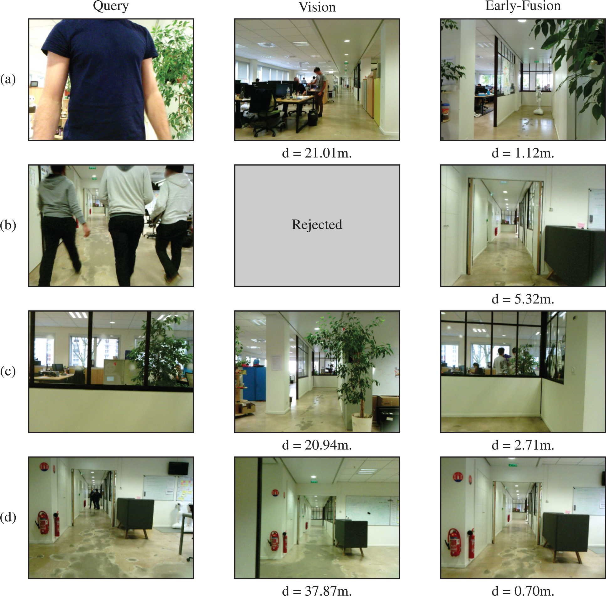
Examples of difficult queries collected in the office building of SoftBank Robotics Europe. Each line shows the query image (left) and the associated location in map computed from classical FABMAP (middle) and early fusion (right) with the associated distances between estimated position and ground truth (below images). The gray image indicates that visual localization considers query (b) as an unknown location.

Therefore, the early fusion system proved to be able of correctly localizing 99.1% of the queries within 20 m of ground truth with the best accuracy. Furthermore, it is worth noting that even if other strategies had higher rejection rates, they did not succeed in catching some aberrant mistakes and early fusion still had the lowest aberrant error rate.

A good example of unacceptable errors is not directly visible in Figure 7(a) and (b). It corresponds to the number of queries that were localized on the wrong floor. These kinds of errors can be particularly problematic in strategies where the result of a global localization is used to load a sub-map of the environment. Nevertheless, it is still a common mistake in environments where floors are very visually similar, such as in hotels or conference centers. In this environment, Figure 9 shows the percentages of queries submitted to this type of error for each tested localization algorithm.

Fig. 9.

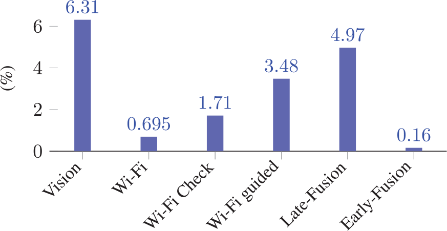
Percentages of queries localized on the wrong floor of the building for each localization algorithms.

Once again, the results in Figure 9 highlight the assistance provided by Wi-Fi. The localization algorithm based only on vision more frequently confused the different floors. It was mistaken about the floor 10 times more often than the localization using Wi-Fi data only. In all fusion schemes, using Wi-Fi helped to reduce these mistakes. However, the early fusion led to a smaller error rate than the Wi-Fi-based localization. These results are particularly interesting because they seem to indicate that the early fusion process results in a better compromise for pose estimation than the other fusion frameworks.

5.4.2. Long-term localization

All the previous results demonstrate the interest of merging Wi-Fi and vision for localizing in this environment. These good performances encouraged some tests in more challenging situations. Thus, the long-term robustness of our approach was also tested. These tests were realized by spacing the initial exploration phase and localization tests 7 months apart. The obtained results plotted in Figure 10(a) and (b) reveal that visual localization had deteriorated more than Wi-Fi localization. This can be easily explained by all the visual transformations that took place during these 7 months. These modifications strongly affected the results of visual and sequential localizations. Conversely, the small changes that occurred in Wi-Fi signals, such as new or missing smartphone APs, were not significant enough to degrade the outcomes of Wi-Fi localization.

Fig. 10.

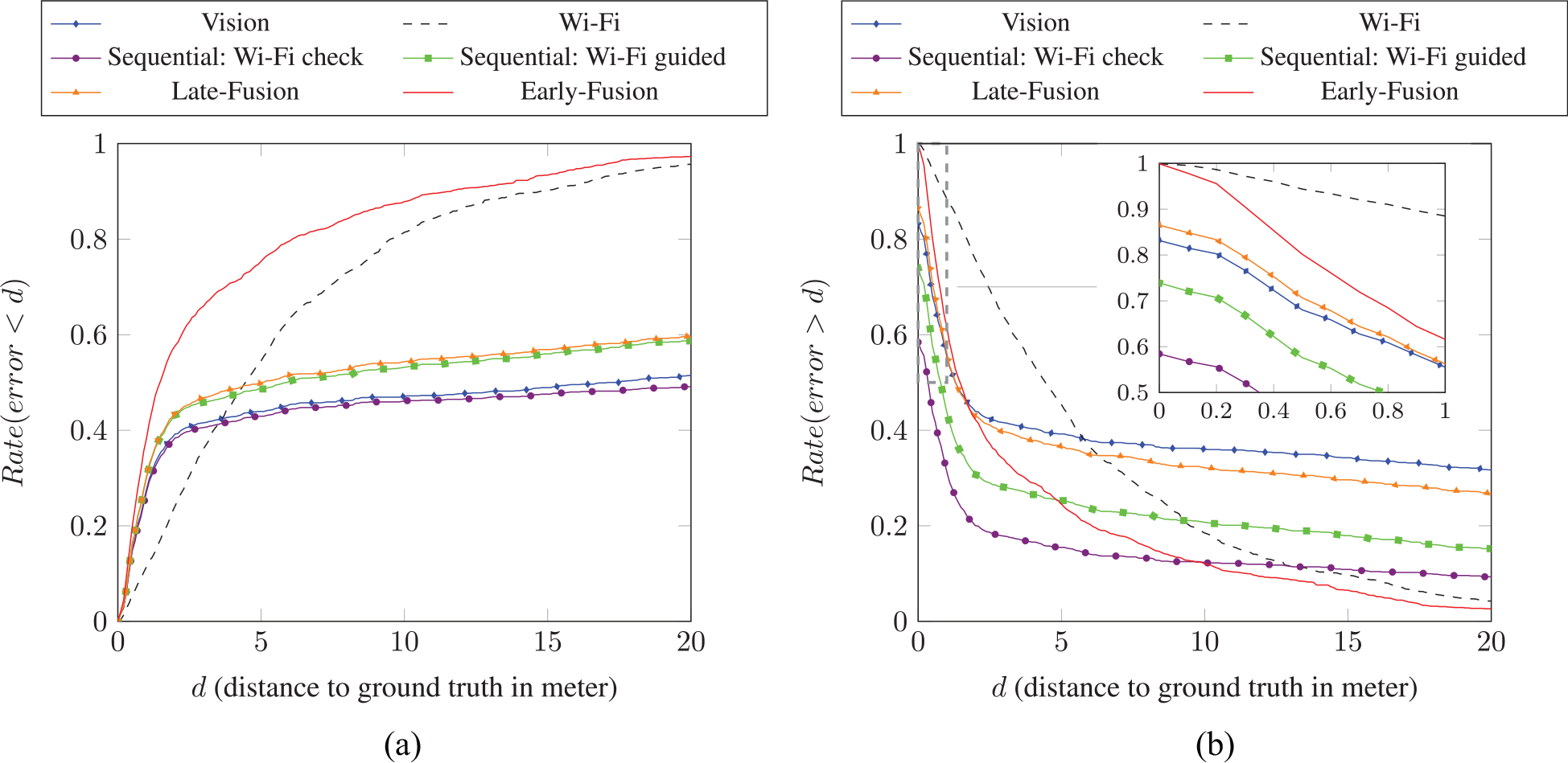
Long-term localization results in the office building of SoftBank Robotics Europe: initial exploration phase and localization tests are acquired seven months apart. (a) Rate of correct localizations. (b) Rate of misplaced localizations.

Values in Table 2 show that our proposed early fusion with Wi-Fi enhanced FABMAP gave the best compromise between visual and Wi-Fi data.

Table 2.

Comparison of the different localization algorithms tested: initial exploration phase and localization tests are acquired 7 months apart.

	Correct localization rate (%) within				Misplaced localization rate (%) away from
	2 m	5 m	10 m	20 m	2 m	5 m	10 m	20 m
Vision	39.2	43.9	47.1	51.4	43.9	39.2	36.0	31.7
Wi-Fi	24.2	54.5	81.4	95.7	75.7	45.4	18.5	4.2
Wi-Fi guided	43.2	48.6	53.2	58.7	30.7	25.3	20.7	15.2
Wi-Fi check	38.4	42.9	46.1	49.1	20.0	15.5	12.3	9.3
Late fusion	43.6	49.9	54.3	59.7	42.9	36.6	32.2	26.8
Early fusion	57.7	75.4	87.9	97.3	42.2	24.5	12.0	2.6

So far, using Wi-Fi data has been shown to be helpful for pose estimation. However, this can be true because of certain aspects of the environment: its visual repetitiveness, its dynamic objects, its large dimensions, and the fact that the Wi-Fi coverage was particularly good with numerous APs. To verify the performances of our early fusion framework in less-favorable conditions, the generality of our algorithm was tested in two other environments.

5.5. Localization with bad Wi-Fi coverage

Some tests were realized in a junior high school. This environment was chosen for several reasons. First, visual localization produced good estimations there. Then, Wi-Fi coverage was not optimal. Only 25 APs were visible compared with 544 in the office building of SoftBank Robotics Europe, for both environments with similar sizes. The 876 m route was run over three different floors with a Pepper robot in the corridors and classrooms of a junior high school. Some examples of images acquired in this environment are shown in Figure 11.

Fig. 11.

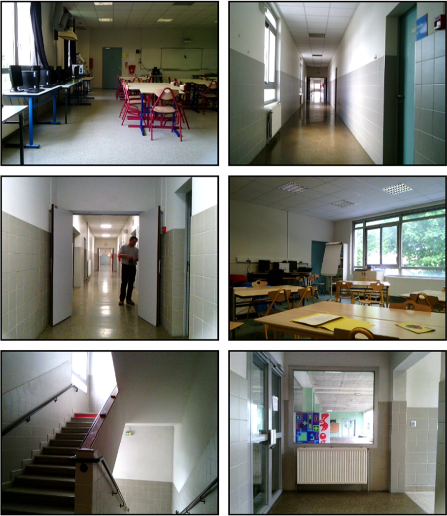
Examples of images acquired in the junior high school test environment.

Figure 12 shows that Wi-Fi localization performances were much worse than those from visual localization. Nevertheless, the good performances of visual FABMAP were not really surprising since the offline learning of our visual vocabulary was realized over the image database presented in Quattoni and Torralba (2009) that contains similar images taken in schools. Collected signatures in this environment were very redundant and empty in some areas, which degraded the Wi-Fi localization. In Section 5.8, performances of Wi-Fi localization are investigated taking into account the strengths of perceived signals.

Fig. 12.

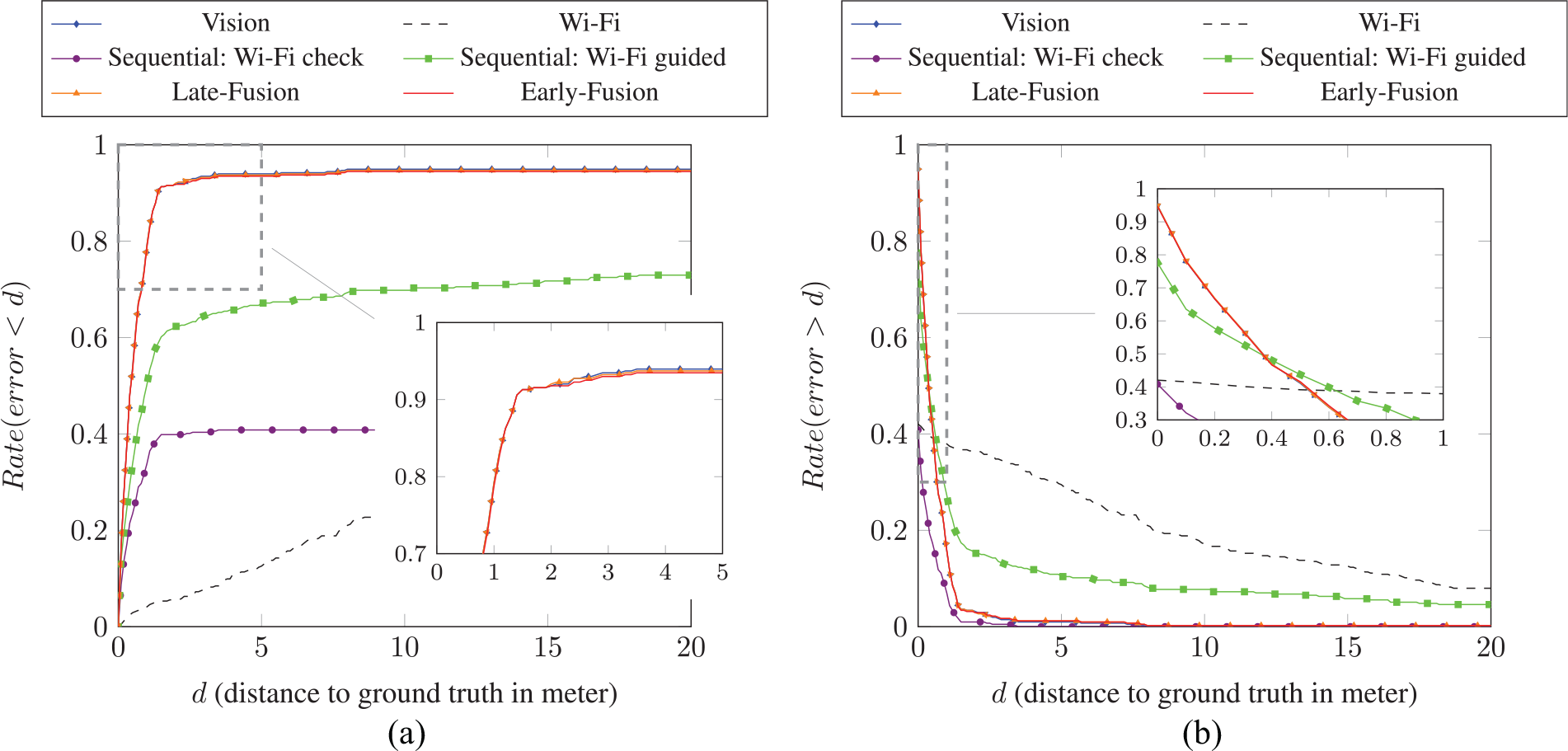
Localization results computed from data collected in a junior high school with bad Wi-Fi coverage. (a) Rate of correct localizations. (b) Rate of misplaced localizations.

Despite the poor accuracy of Wi-Fi localization, early and late fusions did not degrade the results of visual localization in a significant way. The rates of correct and misplaced localization presented in Figure 12(a) and (b) are very similar. However, sequential approaches caused notable deterioration in the performances of the visual localization. Sequential localization with Wi-Fi check became very restrictive and rejects 59.2% of the queries, which strongly degraded its rates of correct localizations (Table 3). For instance, visual localization correctly localized 94.0% of the queries within 5 m of their true positions compared with only 40.8% with the Wi-Fi check sequential approach.

Table 3.

Comparison of classical FABMAP with the presented localization schemes using Wi-Fi data only, and merging visual and Wi-Fi data for operating in a junior high school.

	Correct localization rate (%) within				Misplaced localization rate (%) away from
	2 m	5 m	10 m	20 m	2 m	5 m	10 m	20 m
Vision	91.8	94.0	94.9	94.9	3.0	1.0	0	0
Wi-Fi	5.6	12.6	24.9	34.1	36.5	29.5	17.1	7.8
Wi-Fi guided	62.3	67.1	69.8	72.4	15.2	10.4	7.7	4.6
Wi-Fi check	39.9	40.8	40.8	40.8	1.0	0	0	0
Late fusion	92.0	93.7	94.7	94.7	2.9	1.2	0.2	0.2
Early fusion	91.8	93.5	94.4	94.4	2.9	1.2	0.2	0.2

These results highlight the fact that early fusion from Wi-Fi and visual data seems to not degrade visual localization in environments where Wi-Fi coverage is not optimal.

5.6. Localization in a private apartment

The last environment used during our tests was a private apartment. Owing to its smaller size, testing our algorithm in such environment was interesting to see if the use Wi-Fi would degrade visual localization.

Acquisitions were realized on a single floor and the maximum distance between all the recorded poses was 16 m compared with 76 m in the office building and 65 m in the middle school. In these testing conditions, Wi-Fi coverage was acceptable, with 76 visible APs. Several runs were made and they constituted a total covered distance of 440 m. Some of the paths run by the robot are plotted in Figure 13.

Fig. 13.

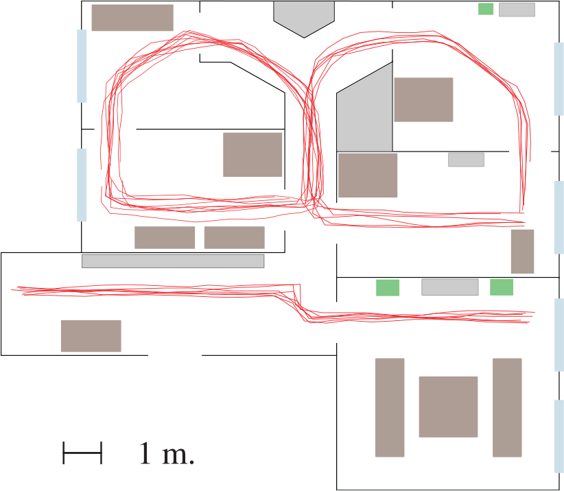
Examples of paths run by a Pepper robot in the different rooms of a private apartment.

Even if this environment was less affected by visual perceptual aliasing, it contained sources of potential errors such as strong variations of brightness and a smaller range of view due to smaller spaces. Some images taken in the apartment are presented in Figure 14.

Fig. 14.

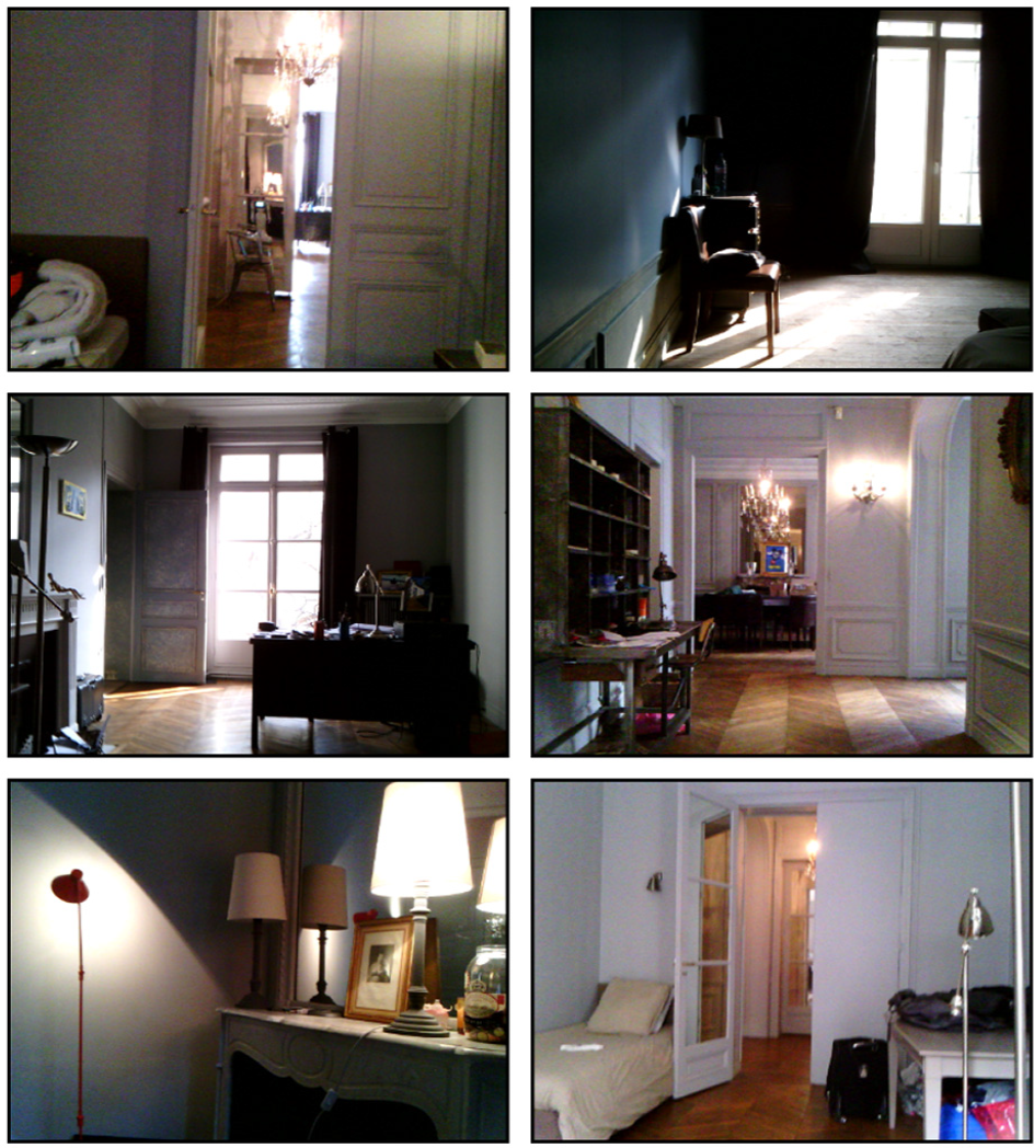
Examples of images acquired in the private apartment test environment.

Without strong visual perceptual aliasing, the localization based on vision produced good results as visible in Figure 15. Thanks to the walls of the different rooms, Wi-Fi signatures were different and localization based only on Wi-Fi data was more accurate in this environment than that achieved in open spaces (Section 5.4.1). Some values of Figure 15(a) and (b) are listed in Table 4.

Fig. 15.

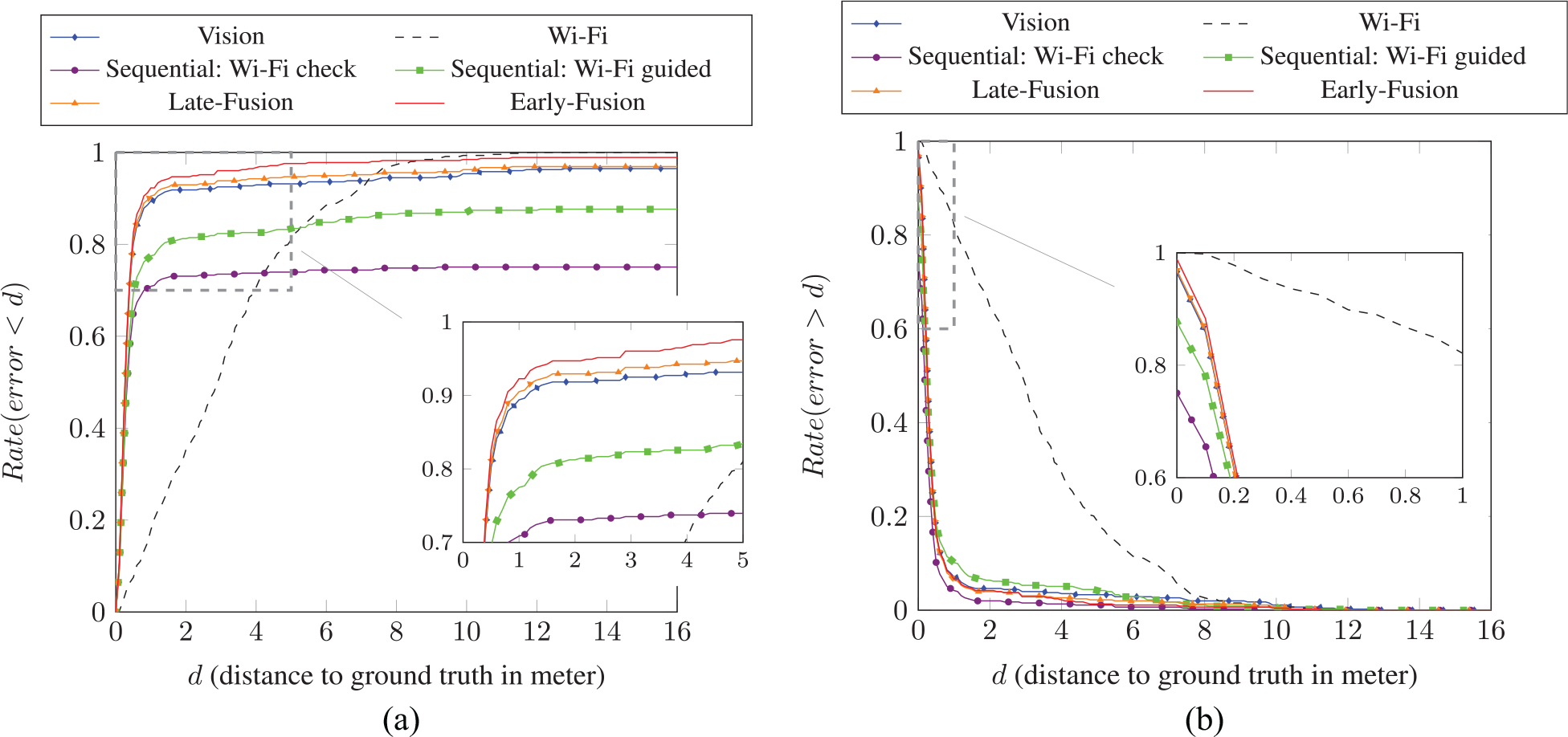
Localization results computed from data collected in a private apartment. (a) Rate of correct localizations. (b) Rate of misplaced localizations.

Table 4.

Comparison of classical FABMAP with the presented localization schemes using Wi-Fi data only, and merging visual and Wi-Fi data for operating in a private apartment.

	Correct localization rate (%) within				Misplaced localization rate (%) away from
	2 m	4 m	6 m	8 m	2 m	4 m	6 m	8 m
Vision	91.8	92.9	93.6	94.4	4.6	3.5	2.8	2.0
Wi-Fi	35.3	70.6	88.5	97.4	64.7	29.4	11.5	2.6
Wi-Fi guided	81.2	82.6	84.8	86.6	6.4	5.0	2.9	1.1
Wi-Fi check	73.0	73.7	74.4	74.8	2.0	1.3	0.6	0.2
Late fusion	92.9	94.3	94.9	95.6	4.0	2.6	2.0	1.3
Early fusion	94.7	96.7	97.8	98.2	4.2	2.2	1.1	0.7

Again, the rate of correct localizations was higher for the early fusion process. The early fusion system also helped to reduce the number of errors. Even if a sequential strategy with Wi-Fi check had smaller error rates (2.0% of misplaced localization further than 2 m from their true positions, against 4.2% for early fusion), it rejected 25.0% of the queries.

5.7. Processing time

Finally, the processing time of a query was computed on Pepper robots. Such robots have a quad-core processor Atom E3845 with a CPU clock rate of 1.91 GHz. The computation times retrieved were similar and around 117 ± 59 ms for all localization algorithms using visual data. Localization based only on Wi-Fi processed a query in about 0.31 ± 0.095 ms. This difference can be explained by the fact that generation of the visual appearance descriptor was longer: 99% of the processing time. This aspect encourages the use of a fast keypoints detector and descriptor to operate in real-time. Note that our implementation was not parallelized.

In these experiments, our system was able to operate in real-time onboard a Pepper robot when acquiring images every 2 s. However, it is still possible to go up to five images per second.

5.8. The application of RSSI

So far, the performances of different localization strategies have been studied without taking into account the intensity of the perceived Wi-Fi signals. As mentioned in Section 3.1, the information carried by the RSSI can be used to improve the accuracy of the localization algorithms using Wi-Fi data. This is done by implementing a kind of discretization of the signal strength that fits the FABMAP formalism. For each known AP, the RSSI is described by multiple binary words. In order to decide how many words to use for encoding the information from the RSSI, Wi-Fi localization results were computed from data collected by multiple Pepper robots in the office building of SoftBank Robotics Europe. This choice can be explained by the good Wi-Fi coverage in this environment with many visible APs, but was still challenging due to the similarity between the collected signatures (see Section 5.4 for more details).

The incremental and exclusive representations presented in Section 3.1 were investigated. Please note that the chosen range of usable intensities was in our case $] - 90 dBm, 0 dBm]$ (as presented in Figure 4) because of Pepper’s hardware and software limitations. Results for localization based on Wi-Fi data only were extracted and some are presented in Table 5. Different numbers of Wi-Fi words were tested to encode the RSSI. The first line of Table 5, for $b = 1$ Wi-Fi word, is the same for both approaches and is used as a reference in the following.

Table 5.

Weight of the number of Wi-Fi words used to describe RSSI coming from each AP for Wi-Fi localization. Results computed with exclusive representation are plotted over gray background and compared to results from the incremental approach proposed in Wietrzykowski et al. (2017).

Number of Wi-Fi words to encode RSSI	Correct localization rate (%) within				Rejection rate (%)
Number of Wi-Fi words to encode RSSI	2 m	5 m	10 m	20 m	Rejection rate (%)
1	26.0	59.7	89.8	98.0	0.7
4	31.3	68.1	92.6	99.1	0.2
	26.1	61.5	90.4	98.9	0.4
8	32.0	70.9	92.9	99.1	0.6
	27.4	67.5	92.9	99.6	0.4
12	29.8	68.9	90.9	97.8	1.0
	28.0	68.8	93.3	99.5	0.4
16	31.2	70.1	91.4	97.5	0.6
	26.6	66.5	91.2	99.7	0.1
20	29.7	65.8	88.0	96.4	1.2
	28.0	65.7	91.5	99.7	0.1

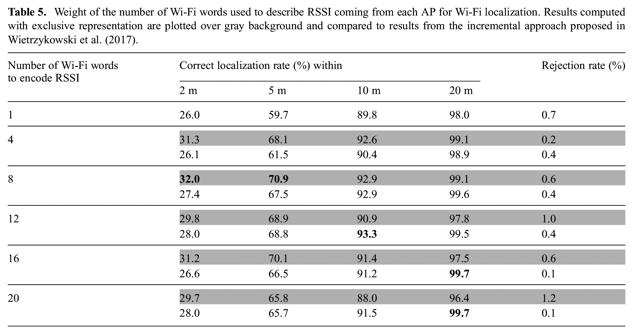
The values presented in Table 5 show that taking into account the information provided by the RSSI improves the accuracy of Wi-Fi localization. Both approaches presented in Section 3.1 were tested. The most accurate localization results were obtained when the RSSI was encoded over eight words. For instance, with each perceived strength described by eight Wi-Fi words, 32.0% of the queries were localized within 5 m of their true positions for the exclusive representation scheme, compared with 26.0% without the use of the RSSI. However, for incremental and exclusive representations, the localization performances were not significantly different.

The use of the RSSI is tested in all presented environments and for all localization strategies using Wi-Fi. The obtained results are presented in tables of performance gains, considering a distance to the ground truth of $d = 5$ m. These gains are expressed in relation with the approach that does not take into account the RSSI; i.e., the method that only considers the presence or absence of known APs in the signature. The values of these gains for the exclusive representation are reported in:

Table 6 for experiments in the SoftBank Robotics Europe office building;

Table 7 for experiments in the junior high school;

Table 8 for experiments in the private apartment;

Table 6.

Impact of exclusive Wi-Fi discretization in the office of SoftBank Robotics Europe. The performance gains are calculated for different numbers b of Wi-Fi words encoding the RSSI of the perceived Wi-Fi signals.

	Gains on correct localization rates within 5 m (%), for different values of b					Impact on misplaced localization rates away from 5 m (%), for different values of b
	$b = 4$	$b = 8$	$b = 12$	$b = 16$	$b = 20$	$b = 4$	$b = 8$	$b = 12$	$b = 16$	$b = 20$
Wi-Fi	+8.6	+11.2	+9.3	+10.4	+6.1	−8.6	−11.2	−9.3	−10.4	−6.1
Wi-Fi guided	−0.3	+0.3	+0.1	−2.3	−3.6	+0.3	−2.5	−3.2	−1.3	−1.3
Wi-Fi check	+0.4	−3.2	−5.7	−7.6	−11.8	−0.2	−3.0	−4.1	−3.6	−4.3
Late fusion	−0.1	+0.1	−0.7	−0.4	−0.1	+0.2	−0.3	+0.4	+0.3	−0.1
Early fusion	+0.9	+2.9	+1.1	+1.0	+1.2	−0.9	−3.0	−1.2	−1.2	−1.6

Table 7.

Impact of exclusive Wi-Fi discretization in the explored junior high school. The performance gains are calculated for different numbers b of Wi-Fi words encoding the RSSI of the perceived Wi-Fi signals.

	Gains on correct localization rates within 5 m (%), for different values of b					Impact on misplaced localization rates away from 5 m (%), for different values of b
	$b = 4$	$b = 8$	$b = 12$	$b = 16$	$b = 20$	$b = 4$	$b = 8$	$b = 12$	$b = 16$	$b = 20$
Wi-Fi	+8.9	+15.7	+9.4	+13.0	+11.8	−8.9	−15.7	−9.4	−13.0	−11.8
Wi-Fi guided	+4.1	−6.3	−9.2	−7.2	−13.5	−4.1	+1.4	+3.6	+1.4	+3.6
Wi-Fi check	+8.2	−4.3	−10.0	−4.1	−10.0	+0.5	−0.2	0	0	−0.2
Late fusion	+0.5	+0.2	0	+0.2	+0.7	−0.2	−0.5	0	−0.2	−0.7
Early fusion	−0.2	+0.2	−0.5	−0.2	0	0	−0.7	0	−0.2	−0.2

Table 8.

Impact of exclusive Wi-Fi discretization in the tested private apartment. The performance gains are calculated for different numbers b of Wi-Fi words encoding the RSSI of the perceived Wi-Fi signals.

	Gains on correct localization rates within 5 m (%), for different values of b					Impact on misplaced localization rates away from 5 m (%), for different values of b
	$b = 4$	$b = 8$	$b = 12$	$b = 16$	$b = 20$	$b = 4$	$b = 8$	$b = 12$	$b = 16$	$b = 20$
Wi-Fi	+3.1	−2.9	+4.0	−0.2	−1.1	−3.1	+2.9	−4.0	+0.2	−1.1
Wi-Fi guided	−6.2	−5.7	+0.2	−8.4	−9.7	−0.4	0	+0.7	+2.9	+3.5
Wi-Fi check	−5.5	−7.7	−2.0	−13.0	−16.3	+0.7	+0.2	+0.4	+0.7	0
Late fusion	+0.7	+0.2	−0.2	+0.4	+0.4	−0.2	0	+0.2	−0.4	0
Early fusion	+0.7	+0.2	−0.4	+1.1	−0.9	−0.2	0	+0.2	−0.7	+0.7

For the experiments carried out in the office building (Table 6) and in the junior high school (Table 7), the use of the RSSI improved the localization performances. The best results are reached by encoding the Wi-Fi signals strengths on $b = 8$ words. However, this improvement is especially significant for the localization using only Wi-Fi data. Approaches merging vision and Wi-Fi are less affected by the use of RSSI, and some of them achieve worse results. For instance, sequential fusion schemes become more restrictive and the performance gains associated with the rate of correct localization are negative.

Regarding the localization results obtained in the apartment, the impact of the RSSI is less favorable (Table 8). In this environment, the closed rooms create enough variations in the Wi-Fi signals so that Wi-Fi localization can be based on a strategy that only takes into account the presence or absence of known APs in a signature. The use of the RSSI adds quantification noise to our system, since Wi-Fi signals are disrupted by the many obstacles they cross, and the measured gains do not point to any clear improvement.

In conclusion, considering the strengths of perceived Wi-Fi signals did not significantly improve the performances of the presented fusion strategies. In addition, encoding RSSI with b Wi-Fi words multiplies the size of the Wi-Fi vocabulary by b. Building Chow Liu tree is a polynomial time algorithm (Chow and Liu, 1968), thus, using RSSI will affect the computing cost of the correlation learning phase. The query phase, on the other hand, has a constant complexity regarding the vocabulary size, thanks to FABMAP2.0. The tradeoff between the extra computational time and the small performance improvement would have to be examined on a case-by-case basis.

6. Conclusion

This article has introduced our early fusion framework. It is a novel approach for merging data from visual and Wi-Fi sensors in order to solve indoor localization tasks for mobile robots.

The presented method has been tested over data collected by multiple Pepper robots with acquisitions schemes following real use cases of these robots. A total distance of 6.4 km has been covered in three different environments: a building office, a junior high school, and a private apartment. In all of these various situations, early fusion has improved the visual localization results. For instance, in an environment where vision faces different problems such as perceptual aliasing or dynamic objects, the improvement of the localization is significant: 90.6% of the queries are correctly localized within 5 m of their true positions, compared with 77.6% with visual localization.

Furthermore, compared with other classical fusion approaches, the early fusion has produced the best results since it improves visual localization results without significantly damaging them even where Wi-Fi signals carry little information. The presented results show that in all our tests, early fusion is the best compromise when merging visual and Wi-Fi data for solving the global localization problem. Some future work could look into qualifying what are the minimal requirements on the environment to obtain good Wi-Fi localization performances.

Footnotes

Appendix. Index to multimedia extensions

Archives of IJRR multimedia extensions published prior to 2014 can be found at http://www.ijrr.org; after 2014 all videos are available on the IJRR YouTube channel at http://www.youtube.com/user/ijrrmultimedia.

SAGE-Journals-Accessible-Video-Player 10.1177/0278364920910485.M1 sj-vid-1-ijr-10.11770278364920910485 Extension 1

Data acquisition and localization process

Acknowledgements

The authors thank Scarlett Fres for her valued help during experimental acquisitions.

Funding

These results have received funding from Bpifrance through the PSPC Project ROMEO 2 and from European Union Horizon 2020 program through the MuMMER project (grant agreement number 688147).

References

Angeli

Filliat

Doncieux

Meyer

(2008) Fast and incremental method for loop-closure detection using bags of visual words. IEEE Transactions on Robotics 24(5): 1027–1037.

Aparicio

Pérez

Bernardos

Casar

(2008) A fusion method based on Bluetooth and WLAN technologies for indoor location. In: IEEE International Conference on Multisensor Fusion and Integration for Intelligent Systems, 2008 (MFI 2008). IEEE, pp. 487–491.

Biswas

Veloso

(2010) Wifi localization and navigation for autonomous indoor mobile robots. In: 2010 IEEE International Conference on Robotics and Automation (ICRA). IEEE, pp. 4379–4384.

Biswas

Veloso

(2013) Multi-sensor mobile robot localization for diverse environments. In: Robot Soccer World Cup. Springer, pp. 468–479.

Boonsriwai

Apavatjrut

(2013) Indoor wifi localization on mobile devices. In: 2013 10th International Conference on Electrical Engineering/Electronics, Computer, Telecommunications and Information Technology (ECTI-CON). IEEE, pp. 1–5.

Chow

Liu

(1968) Approximating discrete probability distributions with dependence trees. IEEE Transactions on Information Theory 14(3): 462–467.

Cummins

Newman

(2008) FAB-MAP: Probabilistic localization and mapping in the space of appearance. The International Journal of Robotics Research 27(6): 647–665.

Cummins

Newman

(2011) Appearance-only slam at large scale with FAB-MAP 2.0. The International Journal of Robotics Research 30(9): 1100–1123.

Glover

Maddern

Warren

Reid

Milford

Wyeth

(2012) OpenFABMAP: An open source toolbox for appearance-based loop closure detection. In: 2012 IEEE International Conference on Robotics and Automation (ICRA). IEEE, pp. 4730–4735.

10.

Chan

SHG

(2016) Wi-Fi fingerprint-based indoor positioning: Recent advances and comparisons. IEEE Communications Surveys and Tutorials 18(1): 466–490.

11.

Howard

Siddiqi

Sukhatme

(2003) An experimental study of localization using wireless ethernet. In: Field and Service Robotics. Springer, pp. 145–153.

12.

Huang

Millman

Quigley

Stavens

Thrun

Aggarwal

(2011) Efficient, generalized indoor WiFi GraphSLAM. In: 2011 IEEE International Conference on Robotics and Automation (ICRA). IEEE, pp. 1038–1043.

13.

Jiang

Yin

(2015) Indoor localization by signal fusion. In: 18th International Conference on Information Fusion.

14.

Jirku

Kubelka

Reinstein

(2016) WiFi localization in 3D. In: 2016 IEEE/RSJ International Conference on Intelligent Robots and Systems (IROS). IEEE, pp. 4551–4557.

15.

Kummerle

Hahnel

Dolgov

Thrun

Burgard

(2009) Autonomous driving in a multi-level parking structure. In: IEEE International Conference on Robotics and Automation, 2009 (ICRA’09). IEEE, pp. 3395–3400.

16.

Lafaye

Gouaillier

Wieber

(2014) Linear model predictive control of the locomotion of Pepper, a humanoid robot with omnidirectional wheels. In: 2014 14th IEEE-RAS International Conference on Humanoid Robots (Humanoids). IEEE, pp. 336–341.

17.

Liu

Gan

Yang

, et al. (2012) Push the limit of WiFi based localization for smartphones. In: Proceedings of the 18th annual international conference on Mobile computing and networking. ACM Press, pp. 305–316.

18.

Liu

Chen

, et al. (2017) Scene recognition for indoor localization using a multi-sensor fusion approach. Sensors 17(12): 2847.

19.

Lowry

Sünderhauf

Newman

, et al. (2016) Visual place recognition: A survey. IEEE Transactions on Robotics 32(1): 1–19.

20.

Lowry

Wyeth

Milford

(2014) Towards training-free appearance-based localization: Probabilistic models for whole-image descriptors. In: 2014 IEEE International Conference on Robotics and Automation (ICRA). IEEE, pp. 711–717.

21.

Lynen

Bosse

Furgale

Siegwart

(2014) Placeless place-recognition. In: 2014 2nd International Conference on 3D Vision (3DV), Vol. 1. IEEE, pp. 303–310.

22.

Mirowski

MacDonald

(2013) SignalSLAM: Simultaneous localization and mapping with mixed WiFi, Bluetooth, LTE and magnetic signals. In: 2013 International Conference on Indoor Positioning and Indoor Navigation (IPIN). IEEE, pp. 1–10.

23.

Nister

Stewenius

(2006) Scalable recognition with a vocabulary tree. In: 2006 IEEE Computer Society Conference on Computer Vision and Pattern Recognition (CVPR’06), Vol. 2. IEEE, pp. 2161–2168.

24.

Nowakowski

Joly

Dalibard

Garcia

Moutarde

(2017) Topological localization using Wi-Fi and vision merged into FABMAP framework. In: 2017 IEEE/RSJ International Conference on Intelligent Robots and Systems (IROS). pp. 3339–3344.

25.

Nowicki

(2014) WiFi-guided visual loop closure for indoor navigation using mobile devices. Journal of Automation Mobile Robotics and Intelligent Systems 8(3): 10–18.

26.

Ocaña

Bergasa

Sotelo

Flores

(2005) Indoor robot navigation using a POMDP based on WiFi and ultrasound observations. In: 2005 IEEE/RSJ International Conference on Intelligent Robots and Systems, 2005 (IROS 2005). IEEE, pp. 2592–2597.

27.

Olivera

Plaza

JMC

Serrano

(2006) WiFi localization methods for autonomous robots. Robotica 24(4): 455–461.

28.

Quattoni

Torralba

(2009) Recognizing indoor scenes. In: IEEE Conference on Computer Vision and Pattern Recognition, 2009 (CVPR 2009). IEEE, pp. 413–420.

29.

Quigley

Stavens

Coates

Thrun

(2010) Sub-meter indoor localization in unmodified environments with inexpensive sensors. In: 2010 IEEE/RSJ International Conference on Intelligent Robots and Systems (IROS). IEEE, pp. 2039–2046.

30.

Rohrig

Kiinemund

(2007) Mobile robot localization using WLAN signal strengths. In: 4th IEEE Workshop on Intelligent Data Acquisition and Advanced Computing Systems: Technology and Applications, 2007 (IDAACS 2007). IEEE, pp. 704–709.

31.

Rosten

Drummond

(2006) Machine learning for high-speed corner detection. In: European Conference on Computer Vision. Springer, pp. 430–443.

32.

Rosten

Porter

Drummond

(2010) Faster and better: A machine learning approach to corner detection. IEEE Transactions on Pattern Analysis and Machine Intelligence 32(1): 105–119.

33.

Rublee

Rabaud

Konolige

Bradski

(2011) ORB: An efficient alternative to SIFT or SURF. In: 2011 IEEE international conference on Computer Vision (ICCV). IEEE, pp. 2564–2571.

34.

Ruiz-Ruiz

Canovas

Munoz

RAR

Alcolea

PELdT

(2011) Using SIFT and WIFI signals to provide location-based services for smartphones. In: International Conference on Mobile and Ubiquitous Systems: Computing, Networking, and Services. Springer, pp. 37–48.

35.

Salton

Buckley

(1988) Term-weighting approaches in automatic text retrieval. Information Processing and Management 24(5): 513–523.

36.

Schwiegelshohn

Nick

Götze

(2013) Localization based on fusion of RFID and stereo image data. In: 2013 10th Workshop on Positioning Navigation and Communication (WPNC). IEEE, pp. 1–6.

37.

Sivic

Zisserman

(2003) Video Google: A text retrieval approach to object matching in videos. In: Proceedings Ninth IEEE International Conference on Computer Vision, 2003. IEEE, pp. 1470–1477.

38.

Stumm

Mei

Lacroix

(2013) Probabilistic place recognition with covisibility maps. In: 2013 IEEE/RSJ International Conference on Intelligent Robots and Systems. IEEE, pp. 4158–4163.

39.

Sünderhauf

Protzel

(2011) Brief-gist-closing the loop by simple means. In: 2011 IEEE/RSJ International Conference on Intelligent Robots and Systems (IROS). IEEE, pp. 1234–1241.

40.

Ulrich

Nourbakhsh

(2000) Appearance-based place recognition for topological localization. In: Proceedings ICRA’00: IEEE International Conference on Robotics and Automation, 2000, Vol. 2. IEEE, pp. 1023–1029.

41.

Werner

Kessel

Marouane

(2011) Indoor positioning using smartphone camera. In: 2011 International Conference on Indoor Positioning and Indoor Navigation (IPIN). IEEE, pp. 1–6.

42.

Wietrzykowski

Nowicki

Skrzypczyński

(2017) Adopting the FAB-MAP algorithm for indoor localization with WiFi fingerprints. In: International Conference on Automation. Springer, pp. 585–594.