A soft manipulator for efficient delicate grasping in shallow water: Modeling,control,and real-world experiments

Abstract

Collecting in shallow water (water depth: ~30 m) is an emerging field that requires robotics for replacing human divers. Soft robots have several promising features (e.g., safe interaction with the environments, lightweight, etc.) for performing such tasks. In this article, we developed an underwater robotic system with a three-degree-of-freedom (3-DoF) soft manipulator for spatial delicate grasping in shallow water. First, we present the design and fabrication of the soft manipulator with an opposite-bending-and-stretching structure (OBSS). Then, we proposed a simple and efficient kinematics method for controlling the spatial location and trajectory of the soft manipulator’s end effector. The inverse kinematics of the OBSS manipulator can be solved efficiently (computation time: 8.2 ms). According to this inverse kinematics method, we demonstrated that the OBSS soft manipulator could track complex two-dimensional and three-dimensional trajectories, including star, helix, etc. Further, we performed real-time closed-loop pick-and-place experiments of the manipulator with binocular and on-hand cameras in a lab aquarium. Hydrodynamic experiments showed that the OBSS soft manipulator produced little force (less than 0.459 N) and torque (less than 0.228 N·m), which suggested its low-inertia feature during the underwater operation. Finally, we demonstrated that the underwater robotic system with the OBSS soft manipulator successfully collected seafood animals at the bottom of the natural oceanic environment. The robot successfully collected eight sea echini and one sea cucumber within 20 minutes at a water depth of around 10 m.

Keywords

Soft robotics underwater grasping inverse kinematics hydrodynamics

1. Introduction

Collecting seafood animals (such as sea cucumbers, sea echini, scallops, etc.) cultivated in shallow water and recycling the underwater pollutants are promising fields that require growing autonomic and robotic technologies. Traditionally, human divers are assigned to manually accomplish these tasks (Figure 1(a)). However, the divers for seafood collecting mostly work within the depth range of 0–30 m; a long period of underwater task would cause severe decompression illness (DCI), including cerebral arterial gas embolism, pneumothorax, vascular and tissue injuries, etc. (Barratt et al., 2002). Robots can reduce diver-related injury and cost by taking their place. Robots also have the potential to scale-up operations, making shallow water seafood harvesting more efficient. Most traditional underwater hydraulic robotic arms are designed for mechanical missions or tasks with heavy payloads (Vasilescu et al., 2010). The rigid material of these arms has challenging issues in the delicate grasping of fragile and squishy objects. The huge inertia of a large-mass rigid arm would induce significant vibrations on the underwater vehicle, posing control challenges during operation (Fernandez et al., 2013). Robots could reduce diver-related injury by taking their place. In particular, soft robots have the potential to scale-up operations, making shallow water seafood harvesting more efficient.

Fig. 1.

(a) Seafood collection by a human diver. (b) Snapshot of the underwater robot system with a soft manipulator for grasping fragile sea animals. Multiple cameras are applied to provide underwater vision. The length of the scale bar is 100 mm. ROV: remotely operated vehicle.

The materials and structures found in nature evolved over billions of years have immense potential to inspire soft robotic devices and systems (Majidi et al., 2013; Stuart et al., 2017; Yim et al., 2018). Recently, increasing studies on soft robotics have focused on underwater applications (Katzschmann et al., 2018; Marchese et al., 2014b; Renda et al., 2012). For example, a soft gripper has been used for biological sampling of coral reefs (Galloway et al., 2016); the origami gripper (Teoh et al., 2018) and nanofiber-reinforced soft actuators (Sinatra et al., 2019) were applied to collecting delicate floating organisms; the jamming gripping was exploited in handling in deep sea (Licht et al., 2017); a soft glove was integrated to teleoperate control of the soft wrist modules for biological underwater grasping (Kurumaya et al., 2018; Phillips et al., 2018); soft robotic octopus arms could achieve free motion underwater (Laschi et al., 2012). Soft robots provide an alternative way to collect these fragile sea animals, due to their properties of compliance and safe interaction. Grasping, moving, and placing the seafood animals using soft robots may provide considerable convenience for the sea farming industry, which also enlightens a real-world underwater application for soft continuum robotics.

It is worth noting that inverse kinematics has long been a challenge for soft continuum robots regarding kinematic control (Rus and Tolley, 2015; Webster and Jones, 2010). Previous studies have reproduced the continuum joint using 3UPS-1PU extensible joints and the Denavit–Hatenberg (DH) method for inverse kinematic modeling (Lakhal et al., 2014; Mahl et al., 2014); Jacobian iteration was applied to determine the inverse kinematics for the soft manipulator in two-dimensional (2D) space (Marchese and Rus, 2016; Marchese et al., 2014a, 2016); machine learning algorithms were proposed to train a single-segment soft actuator (Giorelli et al., 2015; Lee et al., 2017) and a soft manipulator (Jiang et al., 2017) to achieve the desired 2D locomotion. Preliminary attempts on the real-time finite element methods (Duriez, 2013) and visual servo control (Wang et al., 2017) were performed. To generate simple, precise, and computationally efficient inverse kinematics, a natural-cyclic coordinate descent (CCD) algorithm was proposed (Martin et al., 2018). Dynamic motion control was also applied to the soft arms in the air (Della Santina et al., 2018; Katzschmann et al., 2019a, 2019b). However, previous studies have not yet experimentally explored the spatial manipulation with inverse kinematics, particularly for collecting tasks in a natural underwater environment.

To address the challenges in underwater delicate grasping in the field environment and inverse kinematics, we developed an opposite-bending-and-stretching structure (OBSS) soft manipulator. During the inverse kinematics-based operation, the position of the end effector of the OBSS soft manipulator can be controlled in the spatial coordinates, while the orientation of the end effector remains facing vertically down. This proposal of the OBSS soft manipulator provides a simple and efficient solution for the inverse kinematics, as well as pick-and-place control for delicate underwater grasping.

The main contributions of this article are as follows.

We design and fabricate a soft manipulator with an OBSS structure, and propose a simple, computationally efficient, and inverse kinematics solution for the soft manipulator prototype. Trajectory planning and closed-loop grasping control with stereo vision are realized on the OBSS manipulator prototype.

We investigate the hydrodynamics in a lab aquarium and reveal the low-inertia feature of the OBSS soft manipulator when moving underwater. Due to its compliance and lightness, the OBSS soft manipulator generates tiny hydrodynamic forces and torques at the operational speed, which allows pick-and-place tasks with low inertial impact on the small underwater vehicle.

We integrate the OBSS soft manipulator with a four-degree-of-freedom (4-DoF) underwater vehicle for the real-world application – collecting seafood animals in shallow water. With the soft robotic manipulator operating under inverse-kinematics-based control, this robotic prototype successfully collected eight sea urchins and one sea cucumber within 20 minutes at a depth of 10 m in the natural oceanic environment.

The outline is as follows. In Section 2, we detail the design, fabrication, and computationally efficient inverse kinematics of the OBSS soft manipulator with sigmoidal opposing curvature. In Section 3, we conduct trajectories planning in complex three-dimensional (3D) patterns and closed-loop grasping with stereo cameras. We validate the control capabilities of the inverse kinematics and investigate the manipulator’s hydrodynamic functions, including forces and wake flows. We also demonstrate field experiments of grasping seafood animals in a lab pool and a natural shallow water environment at a depth of 10 m. In Section 4, we discuss the OBSS for simplifying the inverse kinematics problem and the application of an underwater robotic system with the soft manipulator.

2. Materials and methods

2.1. System overview

For delicate grasping in shallow water, soft robots have intrinsic compliance, which has advantages for grasping fragile seafood animals (for instance, the sea cucumber has a variable module from ~10 to ~10⁹ Pa, according to Capadona et al., 2008). In order to implement the robotic system for this task, we construct a small underwater robot with an OBSS structure soft manipulator (modules around ~10⁵ Pa), as shown in Figure 1(b). In all the spatial motions, the soft manipulator was constrained in the opposite-bending-and-stretching condition, with the orientation of the end effector remaining facing vertically down. This 3-DoF OBSS soft manipulator was controlled to pick-and-place seafood animals under an inverse kinematics model. A 4-DoF underwater remotely operated vehicle (ROV) is integrated with two cameras, one of which is for grasping from a near top view, while another is for guiding movement from a large side view. Through live cameras, both the underwater soft manipulator and ROV are remotely controlled by the human operator on a boat. The movements of the underwater vehicle are under proportional–integral–derivative (PID) control, which enables swimming and hovering stably. The OBSS soft manipulator was 540 mm in length (the soft arm is 416 mm and the gripper is 124 mm) and 48 mm in diameter, with a total mass of 1,050 g. The robot measures 600 mm long, 500 mm wide, and 300 mm tall, with a weight of 30 kg, and an operating depth of 0–50 m. A collecting basket is located under this robot.

2.2. Design and fabrication of the OBSS soft manipulator

For delicate grasping underwater, the soft manipulator should achieve spatial motions and the structure should be robust. We designed and fabricated a soft modularized underwater manipulator that can move three-dimensionally (Figure 2(a)). The OBSS soft manipulator consists of four parts: two bending segments, one stretching segment, and one soft gripper (Figure 2(b)). The bending and stretching segments of the soft arm and the soft gripper are modularized assembled by 3D printed connectors and universal pneumatic joints. The fabrication and assembling procedure is shown in Figure 3. The cross-section of the bending and stretching segments is designed as a cylinder shape (Gong et al., 2018; Martinez et al., 2013). The bending and stretching segments are fabricated with dragon skin 10 (Shore A hardness of 10) and the soft gripper (Hao et al., 2018) with dragon skin 30 (Shore A hardness of 30). Each bending segment can be actuated via three individual chambers (Figure 2(c)) and the stretching segment via one chamber (Figure 2(d)). In both bending and stretching segments, we include the fiber-reinforced structure (Polygerinos et al., 2015) to reduce radial ballooning of the chambers and achieve large bending curvature when pressurized with the same volume of fluid. The fiber-reinforced structure and the modularized design significantly improved the robustness of the OBSS soft manipulator, which has already been tested underwater for hundreds of hours without damage. The OBSS soft manipulator is actuated and controlled via the multi-channel pneumatic control system, shown in Figure S1. This system could generate pressures separately for all the eight pneumatic chambers according to the inverse kinematic model (Section 2.2).

Fig. 2.

The design and principle mechanics of the underwater soft manipulator. (a) An overall side image of the OBSS soft manipulator (scale bar 50 mm). (b) The OBSS soft manipulator was applied to the modularized design that consisted of two bending segments, a stretching segment, and a soft gripper. θ₁ and θ₂ represent the curvature angles of the two bending segments, and α represents the horizontal angle of the end effector. The manipulator was actuated with an opposing curvature where θ₁ = θ₂ and α = 0. (c) The two bending segments had a joining angle of 180°. In this assembling pattern, for example, chamber 1 (in red) of the first bending segment is in the opposite position to chamber 1 (in red) of the second bending segment, where the intersection angle is 180°. (d) The fiber-reinforced stretching segment. The yellow arrow indicates the direction of elongation. (Color online only.)

Fig. 3.

The fabrication process and assembly of the underwater soft manipulator. (a) Fabrication of the bending module. Firstly, the inner layer with three chambers and a tube channel was fabricated with molds, with threads for fiber reinforcement. The inner actuator was then twined with Kevlar wires and covered with an outer layer mold. The bending module was completed by adding universal joints and pneumatic connectors. (b) Fabrication of the stretching module, which was similar to that of the bending module. After molding the outer layer, we sealed it by molding on a bottom layer. (c) Fabrication of the four-fingered soft gripper. The fingers were fabricated by first molding a top layer and then sealing on a bottom layer. (d) Assembling the OBSS soft manipulator with screws and tubes.

For operating in the 3D domain, the soft manipulator should be controllable. We assemble the two bending segments with an offset angle of 180° (Figure 2(c)). In this assembling approach, for example, chamber 1 (in red) of the first bending segment is opposite to chamber 1 (in red) of the second bending segment. Chamber 1 in both bending segments has an intersection angle of 180°. This geometric condition can also be applied to chambers 2 and 3. This specific design simplifies the opposing motion: by actuating the opposite chambers in the two segments with one-to-one matched pressures, the manipulator can bend in a sigmoidal shape regardless of its deflections. During manipulation, this allows the two bending segments to have the same curvature and form an “S” shape (Figure 2(b)), which simplifies kinematic modeling (see Section 2.3 for details); secondly, it facilitates grasping by maintaining the soft gripper in a vertical position above the ground. Figure 4(a) shows the curvature angles of the two bending segments (θ₁, θ₂) and the intersection angle of the end effector and the horizontal plane (α) during one actuation trial. In addition, we find that θ₁ and θ₂ are nearly equivalent and that α equaled zero at each moment, which confirms the effectiveness of the opposing curvature design. Therefore, we can actuate the OBSS soft manipulator with a sigmoidal opposing curvature that enables control throughout the inverse kinematics-based manipulation process.

Fig. 4.

Kinematics of the OBSS soft manipulator. (a) The two bending segments of the OBSS soft manipulator were always actuated with opposing curvatures. Thus, the curvature angles were always equal (θ₁ = θ₂). (b) The spaces and mappings between them, which define the kinematics of the constant-curvature soft manipulator. Inverse kinematics (f_inv) from the position parameters (x_i, y_i, z_i) to chamber lengths {l_i₁, l_i₂, l_i₃, l_e} via arc parameters {κ_i, φ_i, θ_i} was demonstrated, while the opposite direction indicates the forward kinematics (f_for). (c) Geometric functions in a bending segment, where φ_i represents the deflection angle around the z-axis; θ_i represents the curvature angle around the y-axis; r_i represents the curvature radius. (d) An illustration of the geometric schematic view used to describe the first bending segment (the upper bending segment) of the constant-curvature soft manipulator, where h is the distance between the center point O₁ and the outside surface of a chamber, and l_1j is the chamber length. (e) Chamber lengths of the bending segments as a hysteretic function of the actuation pressure (0–130 kPa) in the pressurization (red) and depressurization (blue). (f) Chamber length of the stretching segment as a hysteretic function of the actuation pressure (0–130 kPa) in the pressurization (red) and depressurization (blue).

2.3. Kinematic modeling of the OBSS soft manipulator

In this section, we will describe the modeling of the kinematics and the inverse kinematics of the OBSS soft manipulator. Figure 5 describes the kinematics of the OBSS soft manipulator. The descriptions of spaces, variables, notations, and terminology in Figures 5(a)–(d) are presented. In the modeling of the forward kinematics (f_for) and inverse kinematics (f_inv), transformations among the actuation space (chamber pressures {p_i₁, p_i₂, p_i₃, p_e}), joint space (chamber lengths {l_i₁, l_i₂, l_i₃, l_e}), configuration space (arc parameters {κ_i, φ_i, θ_i}), and task space (position {x, y, z}) are explored to solve the forward/inverse kinematics problems. More specifically, {p_i₁, p_i₂, p_i₃, p_e} represent the pressure in the chambers and {l_i₁, l_i₂, l_i₃, l_e} indicate the chamber lengths, where for p_ij and l_ij the indexes i = 1, 2 and j = 1, 2, 3 refer to the ith bending segment and the jth chamber, respectively; for p_e and l_e the index e refers to the pressure/length of the stretching segment, respectively. In the ith bending segment, we define the arc parameter φ_i as the deflection angle around the z-axis, θ_i as the curvature angle around the y-axis, and r_i represents the curvature radius of ith bending segment. φ is the deflection angle of the soft manipulator (in particular, φ = φ₁). Here κ_i is defined as the curvature of ith bending segment, where κ_i = r_i⁻¹, and {x, y, z} represents the coordinate of the end effector, whereas (x_i, y_i, z_i) is the coordinate of the end of the ith segment. In addition, h is the radius of the segments. w is the moving distance from the soft manipulator to the z-axis.

Fig. 5.

(a) θ₁, θ₂, and α were verified in one actuation with opposing curvature. The two curvature angles (θ₁, θ₂) were almost equal, and the horizontal angle (α) was zero at each moment. (b) Control location error as a function of operating radius w (0–100 mm). (c) The simulated workspace of the manipulator.

In order to control the position (XYZ coordinates) of the manipulator in the spatial coordinates while maintaining the orientation of the soft gripper facing vertically down, the two bending segments of the OBSS soft manipulator are actuated with sigmoidal opposing curvatures during the inverse kinematics-based manipulation process. Taking the stretching segment into account, the manipulator has three DoFs during inverse kinematics-based manipulation: deflection, bending, and extension. Therefore, the constraints of our inverse kinematics modeling are as given in

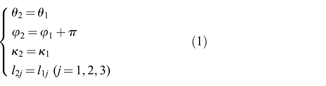
{\begin{matrix} θ_{2} = θ_{1} \\ φ_{2} = φ_{1} + π \\ κ_{2} = κ_{1} \\ l_{2 j} = l_{1 j} (j = 1, 2, 3) \end{matrix}

(1)

The two bending segments of the OBSS soft manipulator are actuated with sigmoidal opposing curvatures. Figure 5(a) provides an overview of the kinematics of the OBSS soft manipulator. The actuation conditions in both chambers are the same, and the curvature angles of both bending segments are always equal (θ₁ = θ₂). Thus, both bending segments together have only two DoFs, deflection angle φ₁ (or φ₂), and curvature angle θ₁ (or θ₂). Including the stretching segment, the manipulator can achieve three DoFs: deflection, bending, and extension.

We modeled the forward kinematics (f_for, solve {x, y, z} according to the given {l_i₁, l_i₂, l_i₃, l_e}) and inverse kinematics (f_inv, solve {l_i₁, l_i₂, l_i₃, l_e} according to the given {x, y, z}). The modeling procedure consists of two steps (Figure 5(b)): the first involves transforming between the end effector coordinates {x, y, z} and chamber length {l_i₁, l_i₂, l_i₃, l_e} coordinates. The essence of this part is how we obtain an inverse solution from three input parameters {x, y, z} to four output parameters {l_i₁, l_i₂, l_i₃, l_e} without other input. The second involves transforming between chamber length {l_i₁, l_i₂, l_i₃, l_e} and pressure {p_i₁, p_i₂, p_i₃, p_e}: the actuation parameter. Owing to the inherent complexity and nonlinear response of the soft materials, solving the second step theoretically poses significant challenges. Instead, we fitted formulas based on the recorded results of pressurization and depressurization experiments with the soft manipulator (Figures 5(e) and (f)). In order to simplify the model, we make the following assumptions.

The bending sections have constant curvatures (5) and the stretching section remain straight (6). The curves are tangent at the intersection points.

The chambers in the same segment are parallel, and the areas of cross-sections are equal in the same section.

2.3.1. Forward kinematics: {x, y, z} ← forwardKin(pi1, pi2, pi3, pe)

The forward kinematics solve the transformation from the chamber pressure {p_i₁, p_i₂, p_i₃, p_e} (actuation space) to the end effector coordinates {x, y, z} (task space), according to Figure 5(b). To acquire the forward kinematics of the manipulator we consider its structure and size. Figures 5(c) and (d) show the modeling of a single segment. We obtain the coordinates of the end effector {x, y, z} from the length of chambers {l_i₁, l_i₂, l_i₃, l_e} through the arc parameters {κ_i, φ_i, θ_i}. According to the geometrics in Figures 5(c) and (d), the transformations from the joint space (chamber lengths {l_i₁, l_i₂, l_i₃, l_e}) to the configuration space (arc parameters {κ_i, φ_i, θ_i}) are as described in

κ_{1} = \frac{1}{r_{1}} = \frac{2 \sqrt{{l_{11}}^{2} + {l_{12}}^{2} + {l_{13}}^{2} - l_{11} l_{12} - l_{11} l_{13} - l_{12} l_{13}}}{(l_{11} + l_{12} + l_{13}) h}

(2)

φ_{1} = \tan^{- 1} (\frac{l_{12} + l_{13} - 2 l_{11}}{\sqrt{3} (l_{12} - l_{13})})

(3)

θ_{1} = \frac{2 \sqrt{{l_{11}}^{2} + {l_{12}}^{2} + {l_{13}}^{2} - l_{11} l_{12} - l_{11} l_{13} - l_{12} l_{13}}}{3 h}

(4)

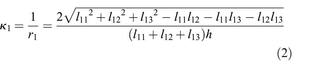
In (2)–(4), h represents the cross-sectional radius, l_1j represents the outer surface length of chambers in the first bending segment, and κ₁ is the curvature. In this study, we used the surface length because it was more accessible for measurement. After finding the arc parameters from the first bending segment, we could obtain the attitudes of the other segments according to (1).

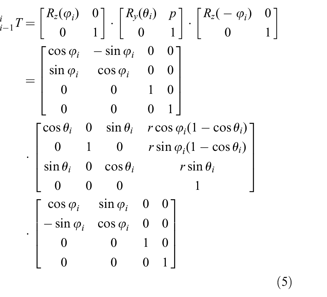
In addition, we can also acquire the end effector coordinates {x, y, z} (task space) from the arc parameters {κ_i, φ_i, θ_i} (configuration space). Mathematically, we consider the manipulator to consist of constant curves (bending segments) and lines (stretching segment) based on the previously stated assumptions. In the bending segments, we describe the bending process in two stages: firstly, the bending segment rotates around the y-axis with θ_i; secondly, the arm rotates around the z-axis with φ_i. Furthermore, we need to post-multiply the homogeneous matrix with the rotation matrix R(–φ_i) and zero translation. The transformation matrix from configuration space to task space for a bending segment is shown in

\begin{matrix} {}_{i - 1}^{i}T = [\begin{matrix} R_{z} (φ_{i}) & 0 \\ 0 & 1 \end{matrix}] \cdot [\begin{matrix} R_{y} (θ_{i}) & p \\ 0 & 1 \end{matrix}] \cdot [\begin{matrix} R_{z} (- φ_{i}) & 0 \\ 0 & 1 \end{matrix}] \\ = [\begin{matrix} \cos φ_{i} & - \sin φ_{i} & 0 & 0 \\ \sin φ_{i} & \cos φ_{i} & 0 & 0 \\ 0 & 0 & 1 & 0 \\ 0 & 0 & 0 & 1 \end{matrix}] \\ \cdot [\begin{matrix} \cos θ_{i} & 0 & \sin θ_{i} & r \cos φ_{i} (1 - \cos θ_{i}) \\ 0 & 1 & 0 & r \sin φ_{i} (1 - \cos θ_{i}) \\ \sin θ_{i} & 0 & \cos θ_{i} & r \sin θ_{i} \\ 0 & 0 & 0 & 1 \end{matrix}] \\ \cdot [\begin{matrix} \cos φ_{i} & \sin φ_{i} & 0 & 0 \\ - \sin φ_{i} & \cos φ_{i} & 0 & 0 \\ 0 & 0 & 1 & 0 \\ 0 & 0 & 0 & 1 \end{matrix}] \end{matrix}

(5)

In the stretching segment, we only need to consider translation along the z-axis with a length of l_e

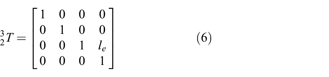
{}_{2}^{3}T = [\begin{matrix} 1 & 0 & 0 & 0 \\ 0 & 1 & 0 & 0 \\ 0 & 0 & 1 & l_{e} \\ 0 & 0 & 0 & 1 \end{matrix}]

(6)

Through the above steps, we are able to describe the transformation of the entire soft manipulator from joint space to task space

{}_{0}^{3}T =_{0}^{1} T \cdot_{1}^{2} T \cdot_{2}^{3} T

(7)

We also found a simple way to calculate the relationship between coordinates (x, y, z), (x₁, y₁, z₁), and (x₂, y₂, z₂): x = x₂ = 2x₁, y = y₂ = 2y₁, and z = z₂+l_e = 2z₁+l_e. With the chamber pressure–length relationship shown in Figures 5(e) and (f), we complete the forward kinematics modeling from actuation space to task space.

2.3.2 Inverse kinematics: {p_i₁, p_i₂, p_i₃, p_e} ←inverseKin(x, y, z)

In inverse kinematics, we solve the chamber pressure {p_i₁, p_i₂, p_i₃, p_e} from the given end effector coordinates {x, y, z}, where the transformation is from task space to actuation space. The coordinate-based control and point-to-point movement of the OBSS soft manipulator can be realized with inverse kinematics. The point-to-point movement is foundational for the manipulator’s picking and placing tasks and trajectory planning. In addition, rapidly solving inverse kinematics problems also helps to improve the real-time control ability of the manipulator. However, the inverse kinematics of soft robots, including continuum ones, remains a challenge (Rus and Tolley, 2015; Webster and Jones, 2010). Finding an inverse solution through solving a number of nonlinear equations in a transformation matrix is a hugely complicated task.

We here propose a rapid inverse solution to the OBSS soft manipulator based on the specific sigmoidal opposing curvature actuation pattern. As discussed above, the manipulator has three DoFs in coordinate space {x, y, z} and four independent chambers {l_i₁, l_i₂, l_i₃, l_e}. In order to address the challenge of obtaining the chamber lengths {l_i₁, l_i₂, l_i₃, l_e} (four outputs) from the coordinates {x, y, z} (three inputs), we implement a constraint condition: at most two chambers in a bending segment are actuated at the same time, so that at least one chamber in each bending segment remains at its initial length. With this constraint, the first step of this approach is determining which chamber was not actuated.

We also resolve the transformation from task space {x, y, z} to joint space {l_i₁, l_i₂, l_i₃, l_e} with the help of the configuration space {κ_i, φ_i, θ_i}. First, we obtain the deflection angle φ₁ from the given inputs {x, y, z}, shown in

φ_{1} = - \tan^{- 1} (\frac{y}{x})

(8)

Then we evaluate φ₁ to determine which chamber is not actuated. The initial length of the chambers {l_i_1int, l_i_2int, l_i_3int, l_eint} could be measured before initiating actuation. Based on the geometric relationship shown in Figures 5(c) and (d), we develop an equation that represents the initial lengths regarding the arc parameters {κ_i, φ_i, θ_i}, in this case when κ_i = r_i⁻¹,

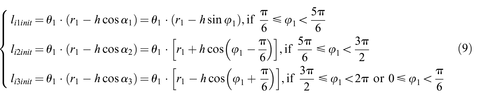
{\begin{matrix} l_{i 1 init} = θ_{1} \cdot (r_{1} - h \cos α_{1}) = θ_{1} \cdot (r_{1} - h \sin φ_{1}), if \frac{π}{6} \leq φ_{1} < \frac{5 π}{6} \\ l_{i 2 init} = θ_{1} \cdot (r_{1} - h \cos α_{2}) = θ_{1} \cdot [r_{1} + h \cos (φ_{1} - \frac{π}{6})], if \frac{5 π}{6} \leq φ_{1} < \frac{3 π}{2} \\ l_{i 3 init} = θ_{1} \cdot (r_{1} - h \cos α_{3}) = θ_{1} \cdot [r_{1} - h \cos (φ_{1} + \frac{π}{6})], if \frac{3 π}{2} \leq φ_{1} < 2 π or 0 \leq φ_{1} < \frac{π}{6} \end{matrix}

(9)

In addition, based on the geometric relationship shown in Figure 5(c), we develop another equation from the given coordinates

\frac{x}{2} = r_{1} \cdot \cos φ_{1} \cdot [1 - \cos θ_{1}]

(10)

In (9) and (10), only r₁ and θ₁ are unknown. Combining the two equations, r₁ and θ₁ can be solved. Then, the calculated arc parameters {κ_i, φ_i, θ_i} provide all of the chamber parameters {l_i₁, l_i₂, l_i₃, l_e}, shown in

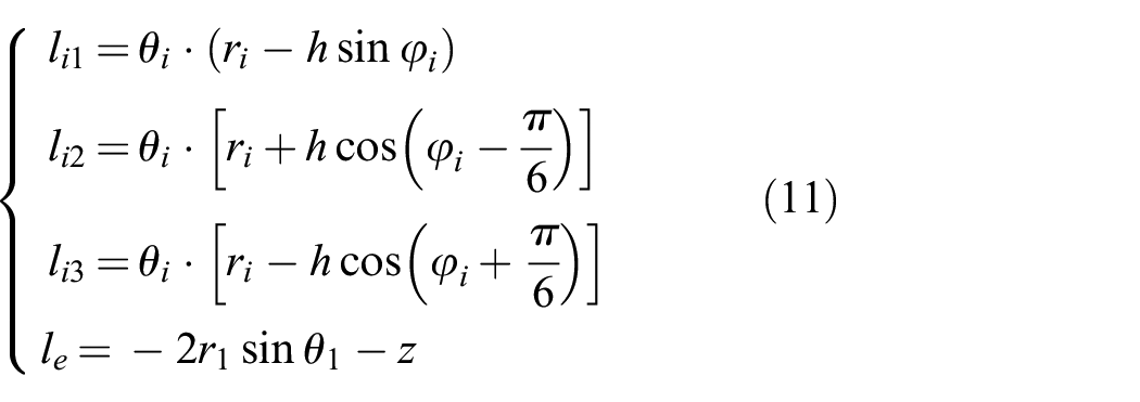
{\begin{matrix} \begin{matrix} l_{i 1} = θ_{i} \cdot (r_{i} - h \sin φ_{i}) \\ l_{i 2} = θ_{i} \cdot [r_{i} + h \cos (φ_{i} - \frac{π}{6})] \\ l_{i 3} = θ_{i} \cdot [r_{i} - h \cos (φ_{i} + \frac{π}{6})] \end{matrix} \\ l_{e} = - 2 r_{1} \sin θ_{1} - z \end{matrix}

(11)

Thus, we obtain a specific inverse transformation from {x, y, z} to {l_i₁, l_i₂, l_i₃, l_e}. Adding in calibrated pressure–length relations (Figures 5(e) and (f)), we can calculate the driving pressure {p_i₁, p_i₂, p_i₃, p_e} from the chamber length {l_i₁, l_i₂, l_i₃, l_e} to complete the model-based control. In the calibration process, to maintain the end effector vertical to the ground, we use a parameter a to adjust the air pressures in the bending segments, shown in

p_{1 j} = a \cdot p_{2 j} - b

(12)

where p_1j is the pressure of the jth chamber in segment 1; p_2j is the pressure of the jth chamber in segment 2. This equation is fitted with the experimental calibration. The experiment suggests that when a = 0.98 and b = −0.63 (linear fitting R² = 0.9994), Equation (12) works for the pneumatics actuation (Figure S3). As a result, the soft manipulator achieves the expected orientation – facing vertical to the ground.

2.3.3. Inverse kinematics control and trajectory planning

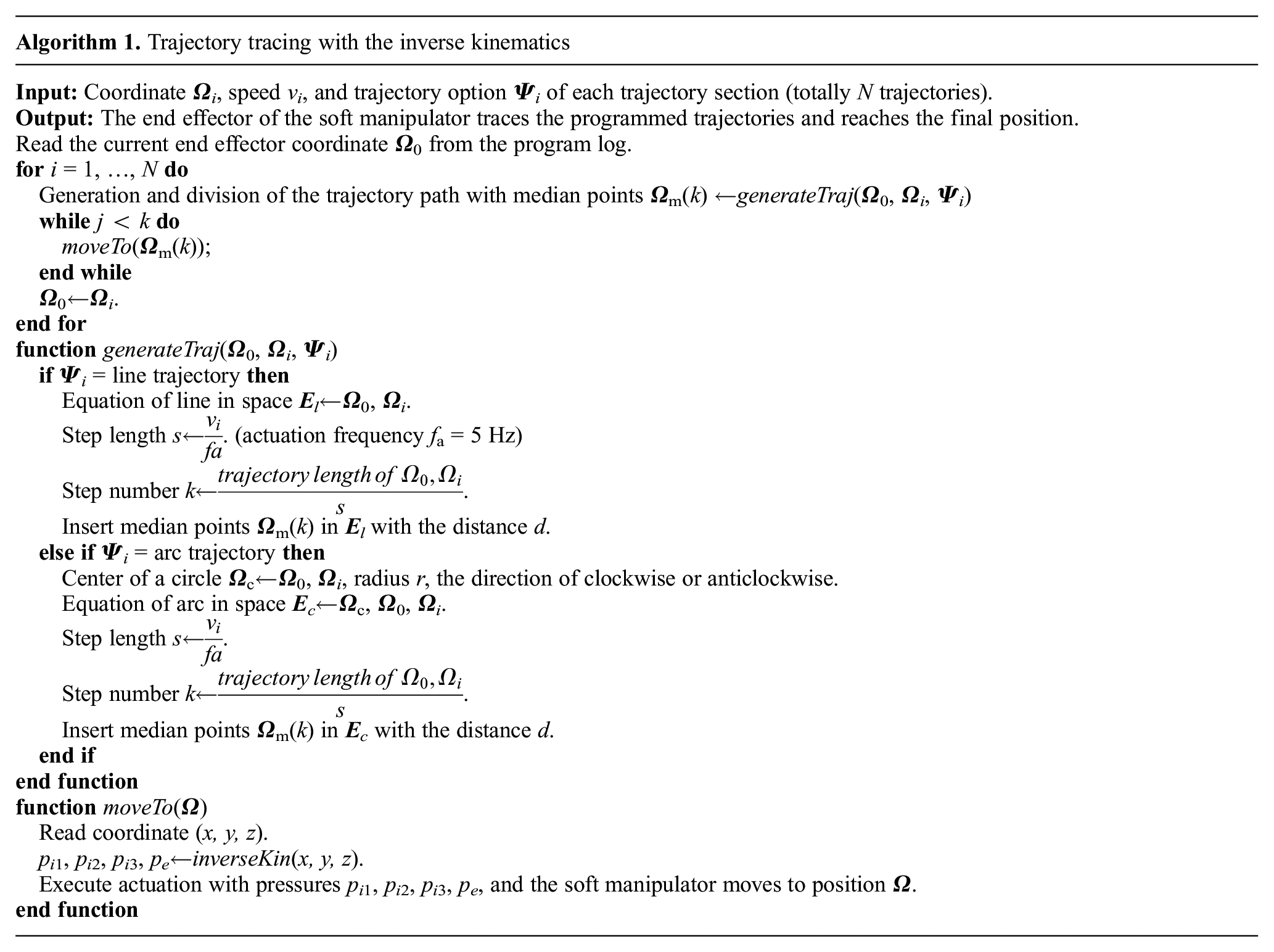
We simulated this inverse kinematic model with the OBSS in MATLAB software, and found that solving chamber lengths {l_i₁, l_i₂, l_i₃, l_e} from the given position {x, y, z} only costs 8.2 ms, which allowed for controlling the soft manipulator in real-time. With the computer interface that integrated the inverse kinematics model (Figure S2), we enabled the coordinate control of the end effector of the OBSS soft manipulator, as well as the trajectory programming with the desired speed. To control the position of the end effector, we inputted the destination coordinates {x, y, z}, and the inverse kinematic model calculated the chamber lengths {l_i₁, l_i₂, l_i₃, l_e}; then the transformed pressures {p_i₁, p_i₂, p_i₃, p_e} were sent to the multi-channel pneumatic control system, and the OBSS soft manipulator was actuated to the desired position.

Applying the inverse kinematic model inverseKin(), as shown in Section 2.3.2, we demonstrate the trajectory control method in Algorithm 1. In the trajectory experiments, we control the soft manipulator to follow the trajectories, which consist of various subdivided patterns. Firstly, the coordinate Ω _i ({x, y, z} of the ith intermediate point that marked subdivided patterns), speed v_i, and trajectory option Ψ _i (line/arc trajectory patterns, radius, and clockwise/anticlockwise direction in the arc trajectory) of each trajectory section were obtained through the human–machine interface. Then, the space equation of each trajectory ( E _l for the line trajectory and for E _c for the arc trajectory) was generated according to the initial coordinate Ω ₀, destination coordinate Ω _i, and trajectory pattern type Ψ _i in procedure generateTraj(), and we divided the trajectory path into a series of the median points Ω _m(k) with a spacing of s. Finally, the inverse kinematics was applied to calculate the pressures and the soft manipulator was actuated to approach the desired point with programmed speed v_i, according to the procedure moveTo(). The definition of the notations can be found in Appendix B.

Algorithm 1. Trajectory tracing with the inverse kinematics
Input: Coordinate Ω _i, speed v_i, and trajectory option Ψ _i of each trajectory section (totally N trajectories).
Output: The end effector of the soft manipulator traces the programmed trajectories and reaches the final position.
Read the current end effector coordinate Ω ₀ from the program log.
for i = 1, …, N do
Generation and division of the trajectory path with median points Ω _m(k) ←generateTraj( Ω ₀, Ω _i, Ψ _i)
while j < k do
moveTo( Ω _m(k));
end while
Ω ₀← Ω _i.
end for
function generateTraj( Ω ₀, Ω _i, Ψ _i)
if Ψ_i = line trajectory then
Equation of line in space E _l← Ω ₀, Ω _i.
Step length s← $\frac{v_{i}}{fa}$ . (actuation frequency f_a = 5 Hz)
Step number k← $\frac{trajectory length of Ω_{0}, Ω_{i}}{s}$ .
Insert median points Ω _m(k) in E _l with the distance d.
else if Ψ_i = arc trajectory then
Center of a circle Ω _c← Ω ₀, Ω _i, radius r, the direction of clockwise or anticlockwise.
Equation of arc in space E _c← Ω _c, Ω ₀, Ω _i.
Step length s← $\frac{v_{i}}{fa}$ .
Step number k← $\frac{trajectory length of Ω_{0}, Ω_{i}}{s}$ .
Insert median points Ω _m(k) in E _c with the distance d.
end if
end function
function moveTo( Ω )
Read coordinate (x, y, z).
p_i₁, p_i₂, p_i₃, p_e←inverseKin(x, y, z).
Execute actuation with pressures p_i₁, p_i₂, p_i₃, p_e, and the soft manipulator moves to position Ω .
end function

2.4. Experimental setup

2.4.1. Trajectory planning with inverse kinematics

In order to evaluate the kinematic modeling, we performed experiments on trajectory planning and characterized the manipulator’s location error. With trajectory step lengths of 10 mm, we tracked location errors of up to 100 mm in the different moving distance (w). We also tested the trajectory planning capabilities by charting different paths, such as a line, circle, star, figure-eight shape, heart, helix, etc., and compared the experimental trajectories with those simulated in MATLAB. We employed a stereo camera system to capture the position of the manipulator while following different motion patterns and paths. The stereo cameras were carefully calibrated with an error of less than 0.5 mm. During the tests, the manipulator was mounted in water and actuated by seven proportional pneumatic valves (ITV0030, SMC, Japan). We obtained marker point coordinates from the different camera views to digitally chart the motion patterns of the manipulator.

2.4.2. Hydrodynamic force measurements

We employed a hydrodynamic measurement platform to record the forces, torque, and wake flow produced by the OBSS soft manipulator’s underwater movements (Figure 6(a)). To avoid interference with the water surface, we mounted the manipulator at mid-depth in the tank. We then used a six-axis force transducer (mini-40, ATI, Canada) to measure the hydrodynamic forces. In the digital particle image velocimetry (DPIV) experiments, a high-speed camera (SP-5000, JAI, Denmark) was used to record images of water flow at a frequency of 250 Hz. The flow was visualized by seeding the water with 10 μm diameter near-neutral buoyant glass beads, which reflected a light sheet from a 4 W, 532 nm wavelength laser. We then obtained the vorticity of each point in the calculation region by using commercial software (MicroVec, LiFangTianDi Inc., China) to process the raw images. We conducted the DPIV experiment and captured a vortex street at a Reynolds number (Re) of 4,800 to examine how the manipulator affected the flow field while conducting picking and placing tasks in the water tank. We also measured the hydrodynamic forces of the cylindrical-shaped manipulator under different flow speeds (10–100 mm/s), Reynolds number (Re) 480–4800. The manipulator was programmed to move in a straight-line trajectory with different amplitudes A (50, 100, 150, and 200 mm) at variable speed v (5–50 mm/s with a 5 mm/s step length).

Fig. 6.

Experimental versus programmed trajectory paths of the end effector’s center point based on the inverse kinematics method. Line (a) and circle (b) trajectories (left-hand subpanel) from points A to B and dynamic responses (right-hand subpanels) at different speeds (10, 20, and 30 mm/s) were performed. The manipulator also traced the two-dimensional outlines of a star (c), figure-eight (d), and heart (e), as well as the three-dimensional trajectories of a helix (insert: a three-quarter view of the helix structure) (f), an inverted rectangular pyramid (insert: a side view of the pyramid) (g), and the letters “BUAA” (abbreviation of Beihang University) (h). The left-hand panels in (c)–(g) and (h) show the quantitative comparison of the desired simulated path (blue line) and the tracked trajectories (red circles) during the experiments, where the black lines indicate the positions and attitudes of the manipulator and the black dots represent the intersections of the segments. The right-hand panels in (c)–(g) show the experimental images with tracked paths in red. More details can be found in supplementary video S1 (Refer to appendix A). (Color online only.)

2.4.3. Closed-loop manipulation through binocular and on-hand cameras

Underwater vision for real-time robot manipulation has long posed challenges for engineers because of degenerated image quality and measurement imprecision due to refringence (Chen et al., 2017). To observe how the manipulator picked and placed objects automatically underwater, we used a binocular camera (ZED, Stereolab, USA) and an on-hand camera to show the positions of the target object and the end effector (Figure 7(a)). The side-view binocular camera was used for full observation to detect the object and navigate the manipulator’s approach. The on-hand camera, which provided a close-up and top-down view, was used for accuracy adjustments after approaching a target. The three-camera system improved measurement accuracy through visual redundancy.

Fig. 7.

Real-time visual feedback control system with inverse kinematic modeling for underwater grasping. (a) Setup of the manipulator with an underwater vision system. A redundant binocular camera and on-hand camera system were employed to enhance the precision of underwater measurements. (b) The closed-loop image processing and actuation procedure in a control loop for underwater grasping. (c) Underwater image before restoration and (d) (red, green, blue) RGB distribution of the image. (e) Restored underwater image and (f) its RGB distribution. ROV: remotely operated vehicle; RUAS: real-time and unsupervised advancement scheme; SSD: Single-shot MultiBox Detector; KCF: kernelized correlation filter. (Color online only.)

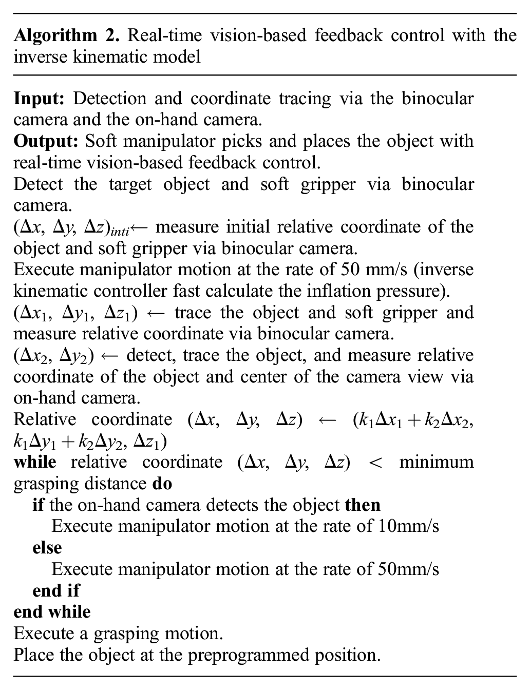
Figure 7(b) illustrates the image processing and actuation procedure control system. We restored the raw images from the binocular camera with a real-time and unsupervised advancement scheme (RUAS) (Chen et al., 2017) for clear and white-balanced visual signals to improve detection performance. We detected the target and gripper with a Single-shot MultiBox Detector (SSD) in an initial frame (Liu et al., 2016), then tracked them with kernelized correlation filters (KCFs) (Henriques et al., 2015). In this way, the coordinate difference between the object and gripper (Δx₁, Δy₁, Δz₁) was obtained. We also applied the same detection and tracking process to the on-hand camera feed to acquire the coordinate difference between the object and center of the gripper (Δx₂, Δy₂) (equal to (null, null) if no object is in view). Lastly, we converted these two coordinates to a final precise coordinate (Δx, Δy, Δz) to actuate the manipulator, given by

{\begin{matrix} Δ x = k_{1} Δ x_{1} + k_{2} Δ x_{2} \\ Δ y = k_{1} Δ y_{1} + k_{2} Δ y_{2} \\ Δ z = Δ z_{1} \end{matrix} k_{1} + k_{2} = 1

(13)

The dynamic weight parameters k₁ and k₂ were dependent on whether the object was in the visual field of the on-hand camera

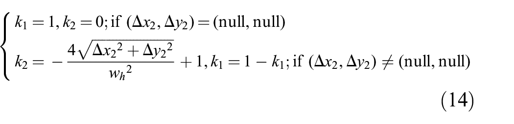
{\begin{matrix} k_{1} = 1, k_{2} = 0; if (Δ x_{2}, Δ y_{2}) = (null, null) \\ k_{2} = - \frac{4 \sqrt{Δ {x_{2}}^{2} + Δ {y_{2}}^{2}}}{{w_{h}}^{2}} + 1, k_{1} = 1 - k_{1}; if (Δ x_{2}, Δ y_{2}) \neq (null, null) \end{matrix}

(14)

The parameter w_h was the width of the on-hand camera view. The closed-loop control architecture is shown in Figure 8(a). The real-time vision-based feedback control with the inverse kinematics algorithm is described in Algorithm 2. In addition, the maximum feedback frequency for processing was 76 Hz. All coordinates of cameras here were unified with the coordinate system of the OBSS soft manipulator. This method left out the underwater calibration of the stereo vision system, which could be applied in a variety of aquatic environments.

Fig. 8.

Real-time vision-based feedback control with the inverse kinematic model for underwater grasping. (a) The closed-loop control architecture. The system consisted of the manipulator, the pneumatic actuation system, and the stereo camera system with binocular and on-hand cameras. The input parameters were the position coordinates generated from the binocular camera. The output parameter was the location of the manipulator’s gripper. Initially, the target object might only be detected by the binocular camera in a full view, which directed the manipulator at high speed. Once the object was detected within the on-hand camera’s view, the manipulator moved with low speed and increased accuracy until the object appeared at the center of the on-hand camera view where the gripper could grasp it. (b)–(e) Demonstration of underwater picking and placing tasks with the aid of visual feedback and inverse kinematics. More details can be found in supplementary video S2 (Refer to appendix A). (Color online only.)

Algorithm 2. Real-time vision-based feedback control with the inverse kinematic model
Input: Detection and coordinate tracing via the binocular camera and the on-hand camera.
Output: Soft manipulator picks and places the object with real-time vision-based feedback control.
Detect the target object and soft gripper via binocular camera.
(Δx, Δy, Δz)_inti← measure initial relative coordinate of the object and soft gripper via binocular camera.
Execute manipulator motion at the rate of 50 mm/s (inverse kinematic controller fast calculate the inflation pressure).
(Δx₁, Δy₁, Δz₁) ← trace the object and soft gripper and measure relative coordinate via binocular camera.
(Δx₂, Δy₂) ← detect, trace the object, and measure relative coordinate of the object and center of the camera view via on-hand camera.
Relative coordinate (Δx, Δy, Δz) ← (k₁Δx₁+k₂Δx₂, k₁Δy₁+k₂Δy₂, Δz₁)
while relative coordinate (Δx, Δy, Δz) < minimum grasping distance do
if the on-hand camera detects the object then
Execute manipulator motion at the rate of 10mm/s
else
Execute manipulator motion at the rate of 50mm/s
end if
end while
Execute a grasping motion.
Place the object at the preprogrammed position.

3. Results

3.1. Trajectory planning with inverse kinematics

We experimentally evaluated the location error and the workspace of the manipulator under the inverse kinematic model. The average control errors are shown in Figure 4(b) when the manipulator was actuated at different distances (w) in different orientations (φ_i). We found that the error remained between 2.7 and 13.4 mm as w varied from 0 to 100 mm in different orientations. These results show that the manipulator performed controllable picking and placing tasks at exact points within a margin of error. The simulated workspace of the manipulator according to our kinematic model is illustrated in Figure 4(c). The model shows that the manipulator can operate within a 3D workspace of 260 mm in length, 240mm in width, and 220 mm in height. The y–z plane-based asymmetry workspace pattern was caused by the different bending orientations and the number of pressurized chambers. In the workspace simulation, we assumed that all the six pressurized chambers in the bending segments can elongate up to 155% according to the calibration results shown in Figure 5(e), as well as 150% for the chamber in the stretching segment, according to Figure 5(f). The workspace was calculated considering the multiple bending orientations of each bending segment, which includes both scenarios of the single internal chamber being actuated and multiple chambers being actuated in a bending segment. In addition, the bending orientations, affected by the actuated chamber numbers, introduced the asymmetries of the workspace pattern. For example, in the x–z plane, the positions where y > 0 represented a single internal chamber that was actuated in a bending segment, while the positions where y < 0 represented the other two chambers that were actuated with equal pressure in a bending segment.

We found that the experimental results matched well with the desired trajectories of straight lines and circles, the most fundamental movement elements. For a linear trajectory (Figure 9(a)), the manipulator was actuated from point A (100, –40, –390) (units are mm with the origin (0, 0, 0) at the base of the manipulator) to point B (–100, 0, –370) at a constant speed of 10 mm/s. The red circles are tracked points from the experiments; the blue line is the simulated path programmed on a computer; the black lines represent the manipulator; the black dots on the black lines represent the junctions of different segments. The results show that the experimental trajectory deviated little from the desired path in 3D space. When the speeds were programmed at 10, 20, and 30 mm/s, the tracked points continued to match the programmed path well with an error smaller than 13.4 mm. For the circle trajectory (Figure 9(b)), the manipulator was actuated from point A (100, 0, –375) to point B (–100, 0, –370) with a clockwise rotation angle of 180°, radius of 100 mm, and constant speed of 10 mm/s. At all speeds (10, 20, and 30 mm/s) the tracked points matched the programmed path closely with an error of smaller than 12.8 mm.

Fig. 9.

Hydrodynamics of the manipulator. (a) Schematic view of the digital particle image velocimetry (DPIV) experimental apparatus: the manipulator was mounted on a six-axis force transducer. A high-speed camera captured the flow field and nylon particles lit by a laser sheet as a force transducer mounted on the end of the arm measured force and torque. (b) Hydrodynamic resistance coefficient C_d versus Reynolds number Re. (c) The DPIV flow field of the soft manipulator at the Reynolds number of 4800.

We also demonstrated that the manipulator could follow complex trajectories. We tested trajectories including 2D patterns such as a star, figure-eight shape, and heart (Figures 9(c)–(e)), 3D paths such as a helix and inverted rectangular pyramid (Figures 9(f) and (g)), and the letters “BUAA” (abbreviation of Beihang University) (Figure 9(h)). All of these trajectories were traced at a constant 10 mm/s. The results demonstrated the manipulator’s capability to follow a wide variety of programmed 2D and 3D trajectories. More details can be found in the supplementary videos S1 – trajectory tracking under the inverse kinematics model.

3.2. Closed-loop manipulation via binocular and on-hand cameras

To validate how the inverse kinematic model could be employed for underwater manipulation, we used the binocular camera and on-hand camera for the closed-loop control. With the help of underwater image restoration with the RUAS, we detected and tracked the objects by the SSD and KCF and actuated the manipulator to grasp an object (sea cucumber) automatically in a lab aquarium tank. When the object was initially detected with the binocular camera (Figure 8(b)), the manipulator was guided quickly (50 mm/s) toward the object by the binocular camera. Once the object appeared in the scope of the on-hand camera (Figure 8(c)), we actuated the OBSS soft manipulator slowly (10 mm/s) according to coordinates from both the binocular and on-hand cameras. When the gripper reached the object, it was inflated to pick it up (Figure 8(d)) and then place it on a target area (green square in Figure 8(e)). More details can be found in the supplementary video S2 – close-looped grasping. In the field test, the RUAS algorithm concentrated on the distribution of the RGB pixels compared with the raw video (Figure 7(d) versus Figure 7(f)). As a result, it significantly enhanced the clarity of the underwater image (especially under turbid water conditions) (Figure 7(c) versus Figure 7(e)) and facilitated object detection during the field test.

3.3. Underwater forces and wake flow

Figure 6(b) shows how resistance coefficient C_d changed with the different moving speeds (v: 10–100 mm/s, Re: 480–4800) of the soft manipulator. The coefficient C_d is defined as

C_{d} = \frac{F}{\frac{1}{2} ρ U^{2} S}

(15)

where F is the measured drag force, ρ is the density of water (1.0184 × 10³ kg/m³), U is the drag speed (from 10 to 100 mm/s), and S is the projected area of the soft manipulator that is vertical to the drag direction. The result showed that the C_d decreased with increasing Reynolds number (Re) from 11.98 to 1.79; this trend agrees well with the basic principle of typical flow around a circular cylinder. The Reynolds number is defined in

Re = \frac{ρ Ud}{μ}

(16)

where ρ is the density of water (1.0184 × 10³ kg/m³), d is the diameter of the soft manipulator (48 mm), and μ is the viscosity coefficient, which we chose as 1.0574 – the viscosity coefficient of water at 18°C, the water temperature during environments. The typical Re of the soft manipulator during underwater manipulation is 50 mm/s, responding to a Re of 2,400.

Figures 10(a) and (b) illustrate how hydrodynamic force and torque of the soft manipulator changed with moving speed (v) and amplitude (A). In each of the three trials, the peak force and torque were recorded. When the manipulator moved at an amplitude of 100 mm, the force increased from 0.172 to 0.402 N (133.7%) as the speed increased from 5 to 50 mm/s. With a similar speed increase at an amplitude of 400 mm, the force also increased from 0.211 to 0.459 N (117.5%), similar to the force increase for 100, 200, and 300 mm amplitudes. The torque (Figure 10(b)) at 400 mm was significantly larger than that at smaller amplitudes, 3.64 times greater than at 100 mm (0.204 compared with 0.056 N·m) at 50 mm/s, and 2.42 times greater at 5 mm/s. When the amplitude was held constant at 400 mm and the velocity was increased from 5 to 50 mm/s, the torque only increased from 0.204 to 0.228 N·m (11.7%). For the circle trajectory (Figures 10(c) and (d)), force and torque showed similar tendencies as with the line trajectory. We also explored how the complex trajectory patterns impacted hydrodynamic forces and torque (Figures 10(e) and (f)). Among the trajectories shown in Figure 9 (figure-eight, heart, helix, star, and “BUAA”), the star produced the greatest force and torque, likely because of the high frequency and large angle of directional changes. To investigate the force induced by the arm mass and the force induced by the fluid drag, separately, the soft manipulator is controlled to move at the velocity of 50 mm/s with a distance of 400 mm following a linear trajectory (Figure S4). During the start and end phases (accelerate and decelerate phases), we observed that the force in the air (induced by the arm mass) played a significant role in the overall force measured underwater. During the steady towing process, the force measured underwater (induced by the hydrodynamic drag) is significantly larger than that measured in air. Therefore, during manipulation, the force is primarily dominated by the inertia (induced by the arm mass) during the accelerating/decelerating, while the force is primarily dominated by the flow velocity (induced by the hydrodynamic drag) during the steady moving state. Figure 6(c) shows the DPIV result that indicates that the generated vortex structure was similar to the typical flow around a cylinder. The boundary layer flow separates from the top/bottom surfaces of the soft manipulator and rolls into discrete vortices, eventually creating a highly turbulent region behind the cylinder. The boundary layer flow separates from the top/bottom surfaces of the soft manipulator and rolls into discrete vortices, eventually creating a highly turbulent region behind the cylinder. These results suggest that in the line and circle trajectories, the amplitude (radius) and velocity both significantly influence the hydrodynamic forces produced, but velocity has a more significant effect on force than amplitude does, while amplitude has a greater effect on torque than velocity does. The trajectory patterns also impacted the force and torque produced. The low force and torque results suggest that the soft manipulator generates low inertia while moving underwater. Thus, the motions, even the rapid movement of the soft manipulator, will cause a low impact on the stability of an underwater vehicle.

Fig. 10.

Hydrodynamic forces measured under different motions of the soft manipulator. Force and torque measurements are shown for a straight-line trajectory (a), (b), and a circle trajectory (c), (d), at different speeds and amplitudes, as well as for other complex trajectories (e), (f).

3.4. Underwater grasping with a remote-controlled rover

To test the capability of the underwater soft manipulator under the inverse kinematics-based control mode, we conducted an underwater robotic system for delicate grasping in shallow water (Figure 1(b)). The OBSS soft manipulator was integrated with a 4-DoF underwater vehicle for the underwater field test. Both the OBSS soft manipulator and underwater robot were under remote control via two real-time underwater cameras (transmitting images via cables) while performing the underwater grasping task. The manual control interface is shown in Figure S2. Underwater grasping was achieved in three steps: (1) the underwater robot was operated to approach the target area and performed hovering and searching for the seafood animal targets, then sank to the bottom of this area (Figure 11(b)); (2) the OBSS soft manipulator was controlled via the inverse kinematics model to approach the seafood animals and pick the target (Figure 11(c)); (3) the OBSS soft manipulator placed the target into the collecting basket and then headed up and repeated from step one to grasp the next object (Figure 11(d)). While working underwater, the pressures in the chambers of the OBSS soft manipulator were balanced according to the water depth. The balancing approach is shown in

p_{d} = p_{0} + ρ_{e} g h_{d}

(17)

where p_d is the pressure applied, p₀ is the originally calculated pressure, ρ_e is the underwater environment density (1,025 kg/m³ is considered as the seawater density), and h_d is the working depth. It should be noted that the OBSS soft manipulator is primarily designed for grasping fragile sea animals, which are typically lightweight to pick up in the water (due to their buoyancy). Currently, we have not yet considered the influence of the gravity and loads on control of the OBSS soft manipulator.

Fig. 11.

Underwater grasping in the lab pool. (a) A close-up and overall view of the robotic system grasping in a still water lab pool. (b)–(d) Underwater grasping procedure in the 5 m depth simulative ocean pool: (b) the robotic system was remotely controlled to approach the target object and sink to the bottom; (c) the soft manipulator located and grasped the target object; (d) the soft manipulator placed the target into the collecting basket while the robotic system floated up. More details can be found in supplementary video S3 (Refer to appendix A).

We performed manipulation tasks by grasping marine seafood animals (sea cucumbers, sea urchins, bivalves, etc.) in the lab pool (Figure 11) and in the natural oceanic environment (Figure 12). Further, we conducted the field seafood collecting experiments at a large seafood farm in a bay area (Bohai, the northeastern part of China), where the seafood animals are well cultivated. In the field test of the natural seabed environment, the underwater grasping robotic system was powered from a ship. The soft manipulator performed controllable motions and delicate grasping the organisms without any damage. It also grasped irregularly shaped sea urchins and a sea cucumber (Figures 12(c) and (d)). As a result, the robotic system successfully collected eight sea urchins and one sea cucumber (Figure 12(e)) within 20 minutes at a water depth of 10 m. Our results showed that the compliance of an underwater soft manipulator could be a promising feature for collecting fragile underwater objects, such as for seafood farming, etc. Movies of the lab tank and natural oceanic grasping experiments are available in the supplementary video S3.

Fig. 12.

The opposite-bending-and-stretching structure soft manipulator grasps seafood animals in the natural sea environments. (a) The procedure for undersea grasping. The robot system was remotely controlled from a carrier ship to dive, grasp, and ascend with seafood. (b) The underwater grasping is demonstrated in the natural undersea environment at 10 m depth. The inserted panel shows the live camera view for manual control. (c)(d) Grasping various undersea animals (sea urchins, sea cucumbers, and bivalves, respectively) with the manipulator. Movies of the underwater grasping experiments in the lab tank and open water are available in supplementary video S3. (e) The result of the undersea grasping: we successfully grasped eight sea urchins and one sea cucumber within 20 minutes.

4. Discussion

4.1. Using the OBSS for simplifying the inverse kinematics problem of the soft manipulator

In this article, we designed the 3-DoF OBSS soft manipulator. The OBSS soft manipulator included two bending segments (bend in the opposing direction with the same curvature), a stretching segment, and a soft gripper. The two bending segments were assembled with an offset angle of 180°, which made uniform the relationship between curvature and chamber pressure in the two bending segments, therefore enabling the inverse kinematic to be solved.

Inverse kinematics of soft continuum robots have attracted researchers’ attention for a long time (Rus and Tolley, 2015; Webster and Jones, 2010), while practical applications in the oceanic environments are a rarity. However, solving higher-order nonlinear equations or training a practical kinematics model in the oceanic environments remains a big challenge; few designs exist beyond laboratory models and prototypes until now. In this study, we proposed a simple, computationally efficient, and inverse kinematics solution for a soft manipulator with an OBSS. The OBSS offers advantages for the kinematic modeling of manipulators since the attitudes of the two bending segments are directly related. As a result, solving the inverse kinematics of a soft manipulator with opposing bending curvature only requires computing geometric functions when modeling the whole manipulator. The OBSS method reduces the total number of pneumatic inputs and requires less computation time and fewer hardware resources. Therefore, this method enhances the practical use of the OBSS manipulator for underwater grasping in the natural environment. For the next step, enabling the orientation angle of the end effector to be controlled would further complement the modeling and control. We expect that this approach also has a broader range of applications envisioned for the future: it may shed light on the control of other soft continuum robots with different actuations and structures, such as tendon-driving manipulators, origami structure-based manipulators, etc.

The efficiency of this inverse kinematic approach allows for the real-time, relatively precise control of the manipulator through positioning, tracking, and grasping tests. This method requires only 8.2 ms to calculate its inverse kinematics in the field, which is comparable with the calculation speed with the natural-CCD algorithm that has represented the most advanced solution until now (approximately 10 ms) (Martin et al., 2018) and machine learning methods (which require training for a long time). In addition, this method enables relatively precise control with a location error (13.4 mm) of less than 2.5% of the manipulator length. In contrast, the DH method generated a 4% error (9 mm) of the total length (Lakhal et al., 2014), and the iteration algorithm generated a 4.8% (9.5 mm) of the total length error (Marchese et al., 2014a). This error is within 25 mm, the error tolerance of the gripper beyond which it would fail to grasp objects successfully (Hao et al., 2018). As a result, this method helps accomplish a range of underwater delicate pick-and-place tasks in oceanic environments.

4.2. The underwater grasping robot system with the OBSS soft manipulator and application

We constructed the OBSS soft manipulator with an underwater vehicle and performed collecting seafood animals in the natural undersea environment. One benefit of applying the soft manipulator is that the compliance allows safely grasping fragile and irregular-shaped objects. The field tests have proven that our soft manipulator was able to collect sea cucumbers, which might be easily damaged by the rigid manipulator. In addition, the soft manipulator was also capable of grasping objects of various shapes and sizes. The lightness of the OBSS soft manipulator offers another advantage for manipulating and grasping underwater, which generates low forces during accelerating/decelerating. Rigid robotic arms and grippers have a relatively large mass that creates significant inertia during locomotion. Big inertia would cause instability for a small underwater rover. Compared with the rigid hydraulic manipulators, the OBSS soft manipulator has a low weight and low inertia. It has a mass of 1.05 kg (almost neutral buoyancy in water) and a length of 540 mm, significantly lighter than the traditional rigid hydraulic manipulators that frequently weigh tens of kilograms, for example, one hydraulic manipulator with a length of 499 mm had a total mass of 17.2 kg (Fernandez et al., 2013). The OBSS soft manipulator operating at 50 mm/s and a 400 mm amplitude generated a hydrodynamic force of 0.459 N and a torque of 0.228 N·m. In contrast, a 695 mm, 3.25 kg rigid underwater arm generated 50 N force and 15 N·m of torque when moving at 0.18 Hz (Nakashima and Takahashi, 2012). Thus, the OBSS soft robot provides a low-inertia manipulator solution for the small, inexpensive underwater vehicle.

The system also displayed a promising ability to grasp soft and delicate objects underwater. Previous studies on undersea grasping soft robots have described soft grippers for reef sampling (Galloway et al., 2016), soft wrist actuators for bending and twisting manipulation (Kurumaya et al., 2018), and a jamming gripper (Licht et al., 2017). By combining a soft manipulator and gripper, our robot can grasp seafood animals safely in a natural underwater environment with kinematical controllability. Our results show that the OBSS soft manipulator offers a promising option for future high-performance, low-cost underwater manipulation systems for marine tasks, including biological sampling, underwater equipment maintenance, recycling pollutants on the seabed, etc. To our knowledge, this work is the first soft manipulator that perform undersea delicate grasping under inverse kinematics-based control.

5. Conclusion

In this article, we designed and fabricated a soft manipulator with the OBSS and integrated the OBSS soft manipulator with an underwater robot system. Simple and computationally efficient inverse kinematics was proposed for grasping soft and delicate objects underwater. The error of the inverse kinematic model-based control was less than 13.4 mm. We validated the trajectory control capabilities of the kinematics by tracking simulated paths of intricate patterns. We then performed underwater grasping guided by real-time closed-loop stereo vision feedback. Hydrodynamic experiments suggested the low-inertia properties of the OBSS soft manipulator, where very little force (0.459 N) and torque (0.228 N·m) were produced while moving underwater. We finally demonstrated that the OBSS soft manipulator grasped seafood animals in a lab pool and a natural seabed environment. The results were that the manipulator successful collected eight sea urchins and one sea cucumber within 20 minutes at 10 m depth of the open sea. Grasping field experiments demonstrated that this manipulator prototype is potentially applicable for grasping delicate objects underwater.

In this study, the sigmoidal opposing curvature design allowed for simple and efficient inverse kinematics, and the vertical grasping mechanism provided adaptability for uneven natural environments. However, this method also reduced the DoFs to three and the overall size of the workspace. Furthermore, pneumatic actuation was used during field tests, which can have a slow response time (based on the length of the pneumatic tubes) that constrains the manipulator’s speed and grasping efficiency. In future studies, one direction is implementing multi-channel hydraulic actuators that can be mounted on board to realize an untethered soft robot. The increased actuation response speed and grasping efficiency will be a further improvement to the current design. Another research direction is investigating the dynamic response of the soft manipulator to compensate for the impacts of ocean currents. Furthermore, enabling the control of the spatial angles of the soft manipulator, which has not been included in this study, would further complement the current robot.

Supplemental Material

IJRR_Supplementary_text_1 – Supplemental material for A soft manipulator for efficient delicate grasping in shallow water: Modeling, control, and real-world experiments

Supplemental material, IJRR_Supplementary_text_1 for A soft manipulator for efficient delicate grasping in shallow water: Modeling, control, and real-world experiments by Zheyuan Gong, Xi Fang, Xingyu Chen, Jiahui Cheng, Zhexin Xie, Jiaqi Liu, Bohan Chen, Hui Yang, Shihan Kong, Yufei Hao, Tianmiao Wang, Junzhi Yu and Li Wen in The International Journal of Robotics Research

Footnotes

Appendix A: Index to Multimedia Extensions

Archives of IJRR multimedia extensions published prior to 2014 can be found at http://www.ijrr.org, after 2014 all videos are available on the IJRR YouTube channel at http://www.youtube.com/user/ijrrmultimedia

SAGE-Journals-Accessible-Video-Player 10.1177/0278364920917203.M1 sj-vid-1-ijr-10.11770278364920917203 Extension 1

A video of an exemplary experimental evaluation from Section 3.1. This video demonstrates the trajectory tracking ability of the OBSS soft manipulator with the inverse kinematics model. The video shows the experiment of the star trajectory tracking.

SAGE-Journals-Accessible-Video-Player 10.1177/0278364920917203.M2 sj-vid-2-ijr-10.11770278364920917203 Extension 2

A video of an exemplary experimental evaluation from Section 3.2. This video demonstrates the real-time, closed-loop grasping with the inverse kinematics model.

SAGE-Journals-Accessible-Video-Player 10.1177/0278364920917203.M3 sj-vid-3-ijr-10.11770278364920917203 Extension 3

A video of exemplary experimental evaluations from Section 3.4. This video demonstrates the field test – the OBSS soft manipulator successfully grasped the seafood animals in the lab pool and natural oceanic environment.

Appendix B: Notation

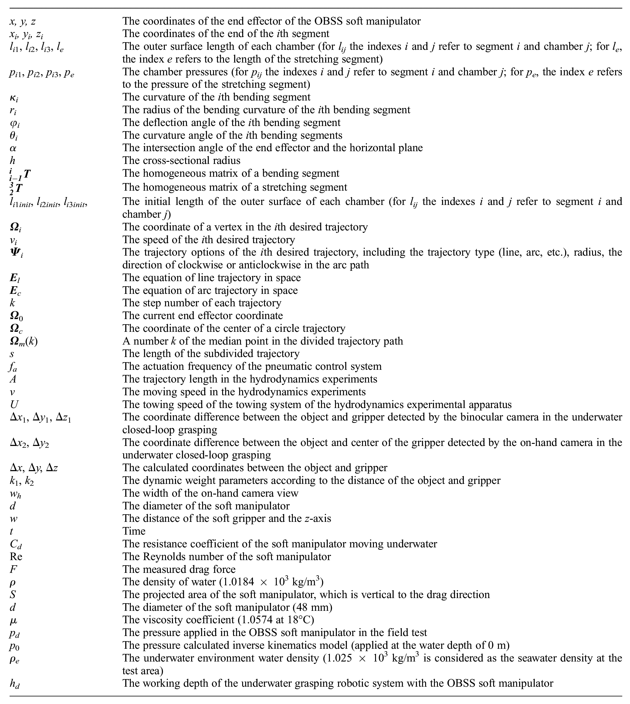
x, y, z	The coordinates of the end effector of the OBSS soft manipulator
x_i, y_i, z_i	The coordinates of the end of the ith segment
l_i ₁, l_i₂, l_i₃, l_e	The outer surface length of each chamber (for l_ij the indexes i and j refer to segment i and chamber j; for l_e, the index e refers to the length of the stretching segment)
p_i ₁, p_i₂, p_i₃, p_e	The chamber pressures (for p_ij the indexes i and j refer to segment i and chamber j; for p_e, the index e refers to the pressure of the stretching segment)
κ_i	The curvature of the ith bending segment
r_i	The radius of the bending curvature of the ith bending segment
φ_i	The deflection angle of the ith bending segment
θ_i	The curvature angle of the ith bending segments
α	The intersection angle of the end effector and the horizontal plane
h	The cross-sectional radius
${}_{i - 1}^{i}T$	The homogeneous matrix of a bending segment
${}_{2}^{3}T$	The homogeneous matrix of a stretching segment
l_i _1init, l_i_2init, l_i_3init,	The initial length of the outer surface of each chamber (for l_ij the indexes i and j refer to segment i and chamber j)
Ω _i	The coordinate of a vertex in the ith desired trajectory
v_i	The speed of the ith desired trajectory
Ψ _i	The trajectory options of the ith desired trajectory, including the trajectory type (line, arc, etc.), radius, the direction of clockwise or anticlockwise in the arc path
E _l	The equation of line trajectory in space
E _c	The equation of arc trajectory in space
k	The step number of each trajectory
Ω ₀	The current end effector coordinate
Ω _c	The coordinate of the center of a circle trajectory
Ω _m(k)	A number k of the median point in the divided trajectory path
s	The length of the subdivided trajectory
f_a	The actuation frequency of the pneumatic control system
A	The trajectory length in the hydrodynamics experiments
v	The moving speed in the hydrodynamics experiments
U	The towing speed of the towing system of the hydrodynamics experimental apparatus
Δx₁, Δy₁, Δz₁	The coordinate difference between the object and gripper detected by the binocular camera in the underwater closed-loop grasping
Δx₂, Δy₂	The coordinate difference between the object and center of the gripper detected by the on-hand camera in the underwater closed-loop grasping
Δx, Δy, Δz	The calculated coordinates between the object and gripper
k ₁, k₂	The dynamic weight parameters according to the distance of the object and gripper
w_h	The width of the on-hand camera view
d	The diameter of the soft manipulator
w	The distance of the soft gripper and the z-axis
t	Time
C_d	The resistance coefficient of the soft manipulator moving underwater
Re	The Reynolds number of the soft manipulator
F	The measured drag force
ρ	The density of water (1.0184 × 10³ kg/m³)
S	The projected area of the soft manipulator, which is vertical to the drag direction
d	The diameter of the soft manipulator (48 mm)
μ	The viscosity coefficient (1.0574 at 18°C)
p_d	The pressure applied in the OBSS soft manipulator in the field test
p ₀	The pressure calculated inverse kinematics model (applied at the water depth of 0 m)
ρ_e	The underwater environment water density (1.025 × 10³ kg/m³ is considered as the seawater density at the test area)
h_d	The working depth of the underwater grasping robotic system with the OBSS soft manipulator

Acknowledgements

We thank Zemin Liu and Wenguang Sun for their contributions to this article. Permission for reusing the material from the previous work of our group (Gong et al., 2018) is authorized by the IEEE.

Declaration of conflicting interests

The authors declared no potential conflicts of interest with respect to the research, authorship, and/or publication of this article.

Funding

The authors disclosed receipt of the following financial support for the research, authorship, and/or publication of this article: This work was supported by the National Science Foundation key projects, China (contracts 61633004, 61822303, and 91848206, 91848105) and in part by the National Key R&D Program of China (Grant No. 18YFB1304600 and 2019YFB1309600).

ORCID iDs

Zheyuan Gong

Xi Fang

Xingyu Chen

Zhexin Xie

Shihan Kong

Junzhi Yu

Supplemental material

Supplemental material for this article is available online.

References

Barratt

Harch

Van Meter

(2002) Decompression illness in divers: A review of the literature. The Neurologist 8(3): 186–202.

Capadona

Shanmuganathan

Tyler

, et al. (2008) Stimuli-responsive polymer nanocomposites inspired by the sea cucumber dermis. Science 319(5868): 1370–1374.

Chen

, et al. (2017) A real-time and unsupervised advancement scheme for underwater machine vision. In: IEEE international conference on cyber technology automation control and intelligent system, Honolulu, USA, 31 July–4 August 2017, pp.271–276. IEEE.

Della Santina

Katzschmann

Biechi

, et al. (2018) Dynamic control of soft robots interacting with the environment. In: 2018 IEEE international conference on soft robotics (RoboSoft), Livorno, Italy, 24–28 April 2018, pp.46–53. IEEE.

Duriez

(2013) Control of elastic soft robots based on real-time finite element method. In: IEEE international conference on robotics & automation, Karlsruhe, Germany, 6–10 May 2013, pp.3982–3987. IEEE.

Fernandez

Prats

Sanz

, et al. (2013) Grasping for the seabed: Developing a new underwater robot arm for shallow-water intervention. IEEE Robotics & Automation Magazine 20(4): 121–130.

Galloway

Becker

Phillips

, et al. (2016) Soft robotic grippers for biological sampling on deep reefs. Soft Robotics 3(1): 23–33.

Giorelli

Renda

Calisti

, et al. C (2015) Neural network and Jacobian method for solving the inverse statics of a cable-driven soft arm with nonconstant curvature. IEEE Transactions on Robotics 31(4): 823–834.

Gong

Cheng

, et al. (2018) An inverse kinematics method of a soft robotic arm with three-dimensional locomotion for underwater manipulation. In: 2018 IEEE international conference on soft robotics (RoboSoft), Livorno, Italy, 24–28 April 2018, pp.516–521. IEEE.

10.

Hao

Gong

Xie

, et al. (2018) A soft pneumatic robotic gripper with variable effective length. Journal of Bionic Engineering 15(2): 220–235.

11.

Henriques

Caseiro

Martins

, et al. (2015) High-speed tracking with kernelized correlation filters. IEEE Transactions on Pattern Analysis and Machine Intelligence 37(3): 583–596.

12.

Jiang

Wang

Liu

, et al. (2017) A two-level approach for solving the inverse kinematics of an extensible soft arm considering viscoelastic behavior. In: IEEE international conference on robotics and automation, Singapore, 29 May–3 June 2017, pp.6127–6133. IEEE.

13.

Katzschmann

Della Santina

Toshimitsu

, et al. (2019a) Dynamic motion control of multi-segment soft robots using piecewise constant curvature matched with an augmented rigid body model. In: 2019 IEEE international conference on soft robotics (RoboSoft). Seoul, Korea (South), 14–18 April 2019. IEEE.

14.

Katzschmann

DelPreto

MacCurdy

, et al. (2018) Exploration of underwater life with an acoustically controlled soft robotic fish. Science Robotics 3(13): eaar3449.

15.

Katzschmann

Thieffry

Goury

, et al. (2019b) Dynamically closed-loop controlled soft robotic arm using a reduced order finite element model with state observer. In: 2019 IEEE international conference on soft robotics (RoboSoft), Seoul, Korea (South), 14–18 April 2019. IEEE.

16.

Kurumaya

Phillips

Becker

, et al. (2018) A modular soft robotic wrist for underwater manipulation. Soft Robotics 5(4): 399–409.

17.

Lakhal

Melingui

Chibani

, et al. (2014) Inverse Kinematic modeling of a class of continuum bionic handling arm. In: 2014 IEEE/ASME international conference on advanced intelligent mechatronics (AIM), Besacon, France, 8–11 July 2014, pp.1337–1342. IEEE.

18.

Laschi

Cianchetti

Mazzolai

, et al. (2012) Soft robot arm inspired by the octopus. Advanced Robotics 26(7): 709–727.

19.

Lee

Leong

, et al. (2017) Nonparametric online learning control for soft continuum robot: An enabling technique for effective endoscopic navigation. Soft Robotics 4(4): 324–337.

20.

Licht

Collins

Mendes

, et al. (2017) Stronger at depth: Jamming grippers as deep sea sampling tools. Soft Robotics 4(4): 305–316.

21.

Liu

Anguelov

Erhan

, et al. (2016) SSD: Single Shot MultiBox Detector. In: Computer Vision – ECCV 2016. Lecture Notes in Computer Science (eds Leibe

Matas

Sebe Nand Welling

), Amsterdam, The Netherlands, 8–16 October 2016, pp. 21–37, vol 9905. Cham: Springer.

22.

Mahl

Hildebrandt

Sawodny

(2014) A variable curvature continuum kinematics for kinematic control of the bionic handling assistant. IEEE Transactions on Robotics 30(4): 935–949.

23.

Majidi

Shepherd

Kramer

, et al. (2013) Influence of surface traction on soft robot undulation. The International Journal of Robotics Research 32(13): 1577–1584.

24.

Marchese

Komorowski

Onal

, et al. (2014a) Design and control of a soft and continuously deformable 2D robotic manipulation system. In: IEEE international conference on robotics & automation, Hong Kong, China, 31 May–7 June 2014, pp.2189–2196. IEEE.

25.

Marchese

Onal

Rus

(2014b) Autonomous soft robotic fish capable of escape maneuvers using fluidic elastomer actuators. Soft Robotics 1(1): 75–87.

26.

Marchese

Rus

(2016) Design kinematics and control of a soft spatial fluidic elastomer manipulator. The International Journal of Robotics Research 35(7): 840–869.

27.

Marchese

Tedrake

Rus

(2016) Dynamics and trajectory optimization for a soft spatial fluidic elastomer manipulator. The International Journal of Robotics Research 35(8): 1000–1019.

28.

Martin

Barrientos

del Cerro

(2018) The natural-CCD algorithm, a novel method to solve the inverse kinematics of hyper-redundant and soft robots. Soft robotics 5(3): 242–257.

29.

Martinez

Branch

Fish

, et al. (2013) Robotic tentacles with three-dimensional mobility based on flexible elastomers. Advanced Materials 25(2): 205–212.

30.

Nakashima

Takahashi

(2012) Clarification of unsteady fluid forces acting on limbs in swimming using an underwater robot arm. Journal of Fluid Science and Technology 7(1): 114–128.

31.

Phillips

Becker

Kurumaya

, et al. (2018) A dexterous glove-based teleoperable low-power soft robotic arm for delicate deep-sea biological exploration. Scientific Reports 8(1): e0200386.

32.

Polygerinos

Wang

Overvelde

, et al. (2015) Modeling of soft fiber-reinforced bending actuators. IEEE Transactions on Robotics 31(3): 778–789.

33.

Renda

Cianchetti

Giorelli

, et al. (2012) A 3D steady-state model of a tendon-driven continuum soft manipulator inspired by the octopus arm. Bioinspiration & Biomimetics 7(2): 025006.

34.

Rus

Tolley

(2015) Design fabrication and control of soft robots. Nature 521(7553): 467–475.

35.

Sinatra

Teeple

Vogt

, et al. (2019) Ultragentle manipulation of delicate structures using a soft robotic gripper. Science Robotics 4(33): eaax5425.

36.

Stuart

Wang

Khatib

, et al. (2017) The Ocean One hands: An adaptive design for robust marine manipulation. The International Journal of Robotics Research 36(2): 150–166.

37.

Teoh

Phillips

Becker

, et al. (2018) Rotary-actuated folding polyhedrons for midwater investigation of delicate marine organisms. Science Robotics 3(20): eaat5276.

38.

Vasilescu

Detweiler

Doniec

, et al. (2010) Amour v: A hovering energy efficient underwater robot capable of dynamic payloads. International Journal of Robotics Research 29(5): 547–570.

39.

Wang

Yang

Liu

, et al. (2017) Visual servoing of soft robot manipulator in constrained environments with an adaptive controller. IEEE/ASME Transactions on Mechatronics 22(1): 41–50.

40.

Webster

III Jones

(2010) Design and kinematic modeling of constant curvature continuum robots: A review. International Journal of Robotics Research 29(13): 1661–1683.

41.

Yim

Sung

Miyashita

, et al. (2018) Animatronic soft robots by additive folding. International Journal of Robotics Research 37(6): 611–628.

Supplementary Material

Please find the following supplemental material available below.

For Open Access articles published under a Creative Commons License, all supplemental material carries the same license as the article it is associated with.

For non-Open Access articles published, all supplemental material carries a non-exclusive license, and permission requests for re-use of supplemental material or any part of supplemental material shall be sent directly to the copyright owner as specified in the copyright notice associated with the article.

0.00 MB

3.48 MB

A soft manipulator for efficient delicate grasping in shallow water: Modeling,control,and real-world experiments

Abstract

Keywords

1. Introduction

2. Materials and methods

2.1. System overview

2.2. Design and fabrication of the OBSS soft manipulator

2.3. Kinematic modeling of the OBSS soft manipulator

2.3.1. Forward kinematics: {x, y, z} ← forwardKin(pi1, pi2, pi3, pe)

2.3.2 Inverse kinematics: {pi1, pi2, pi3, pe} ←inverseKin(x, y, z)

2.3.3. Inverse kinematics control and trajectory planning

2.4. Experimental setup

2.4.1. Trajectory planning with inverse kinematics

2.4.2. Hydrodynamic force measurements

2.4.3. Closed-loop manipulation through binocular and on-hand cameras

3. Results

3.1. Trajectory planning with inverse kinematics

3.2. Closed-loop manipulation via binocular and on-hand cameras

3.3. Underwater forces and wake flow

3.4. Underwater grasping with a remote-controlled rover

4. Discussion

4.1. Using the OBSS for simplifying the inverse kinematics problem of the soft manipulator

4.2. The underwater grasping robot system with the OBSS soft manipulator and application

5. Conclusion

Supplemental Material

IJRR_Supplementary_text_1 – Supplemental material for A soft manipulator for efficient delicate grasping in shallow water: Modeling, control, and real-world experiments

Footnotes

Appendix A: Index to Multimedia Extensions

Appendix B: Notation

Acknowledgements

Declaration of conflicting interests

Funding

ORCID iDs

Supplemental material

References

Supplementary Material

2.3.2 Inverse kinematics: {p_i₁, p_i₂, p_i₃, p_e} ←inverseKin(x, y, z)