
Abstract
In this work, we consider the multi-image object matching problem in distributed networks of robots. Multi-image feature matching is a keystone of many applications, including Simultaneous Localization and Mapping, homography, object detection, and Structure from Motion. We first review the QuickMatch algorithm for multi-image feature matching. We then present NetMatch, an algorithm for distributing sets of features across computational units (agents) that largely preserves feature match quality and minimizes communication between agents (avoiding, in particular, the need to flood all data to all agents). Finally, we present an experimental application of both QuickMatch and NetMatch on an object matching test with low-quality images. The QuickMatch and NetMatch algorithms are compared with other standard matching algorithms in terms of preservation of match consistency. Our experiments show that QuickMatch and Netmatch can scale to larger numbers of images and features, and match more accurately than standard techniques.
1. Introduction
Matching is a fundamental operation common in robotics and computer vision algorithms such as Structure from Motion (SfM), Simultaneous Localization and Mapping (SLAM), and object detection and tracking. Matching in these domains is typically performed on feature descriptors (such as Scale Invariant Feature Transform (SIFT), Oriented FAST and Rotated BRIEF (ORB), and Speeded Up Robust Features (SURF) by Lowe (2004), Rublee et al. (2011), and Bay et al. (2008), respectively) which extract discriminative characteristics from high-dimensional data (i.e., an image). At a fundamental level, these features are used to associate unique objects in the universe to their appearance in multiple views. These different views might be acquired by a geographically dispersed camera or robotic network, which can produce large amounts of data. It is therefore important to have the ability to match features across multiple images (i.e., perform multi-image matching) efficiently, consistently, accurately, and, ideally, in a distributed manner. For instance, match quality is key in settings such as SfM and SLAM, because the quality of the reconstruction is a direct result of how well the features match across images. The speed of image matching is extremely critical in applications such as real-time object detection. Matching consistency of features across many images is also critical for SfM and SLAM since feature points must be tracked not just between images, but across multi-image sequences for the best results. The pervasiveness of graphical processing units (GPUs), networked systems, distributed robotics, cloud computing, and multi-core processors has made the distributability of computer vision solutions relevant to their applicability. These tools have also shown great advantages in speed and bandwidth for other classic algorithms (Garcia et al., 2010; Warn et al., 2009). To this end, we introduce a novel version of our matching algorithm that distributes the computational load of the feature matching problem over multiple agents; the resulting algorithm can handle considerably more features, with only a slight performance loss, while minimizing the amount of necessary communications across nodes.
1.1. Problem overview and contributions
We propose a solution to the following problem: given a set of images taken from a team of robots or a camera network, match unique object features in a distributed manner, as they appear and disappear in the images taken from multiple perspectives. This problem arises often in object detection, localization, and tracking (Bradski, 2000; Cunningham et al., 2012; Zhou et al., 2015), homography estimation (Szeliski, 2010), SfM (Hartley and Ziserman, 2017), and formation control (Montijano et al., 2016). Solutions to this problem are traditionally computationally complex, and often mismatch features when considering more than two images (Bradski, 2000; Lowe, 2004), by either missing matches between two or more views of the same entity in the universe, or by introducing associations between separate universe entities. Multi-image correspondences allow for greater match reliability and a more accurate representation of objects in the universe. Our proposed solution leverages a relatively recent algorithm, QuickMatch (Tron et al., 2017), to quickly and reliably discover correspondences across multiple images. The experiments presented in this article benchmark QuickMatch’s performance by tracking a target object and estimating its trajectory under realistic conditions (i.e., over images with clutter, repeated structures, and poor image quality). We then propose NetMatch, an extension of QuickMatch to a distributed computation setting, which largely preserves match quality while minimizing communication across agents.
1.2. Related work
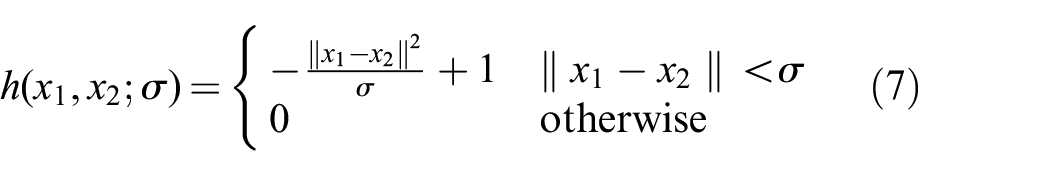
Feature matching is a basic step in many computer vision algorithms. Pairwise matching is the classical approach to this task, where feature descriptors between two images are compared based on a distance metric (e.g., Euclidean or Manhattan distance), and declared a match if this distance is below some threshold (Lowe, 2004; Vedaldi and Fulkerson, 2008). Pairwise matching is often posed as a nearest-neighbor search problem (Dollar and Zitnick, 2013; Garcia et al., 2010). This method is used in two standard algorithms, Brute Force (BF) matching (Bradski, 2000), and Fast Library for Approximate Nearest Neighbors (FLANN) matching (Muja and Lowe, 2014). Pairwise matching has difficulties consistently matching entities with repetitive structure or similar appearance (e.g., adjacent windows on a building facade) because the distance metric alone does not consider the distinctiveness (smallest distance between features from the same image) of the features. Including distinctiveness of features during matching has been shown to be beneficial (Lowe, 2004). For multi-image matching, pairwise matches scale poorly with the number of images and across multiple images, and match correspondences often do not belong to the same ground-truth object (and, hence, link together correspondences between different entities). Graph matching has also been used for pairwise matching. This approach attempts to match vertices (features) and edges (matches) simultaneously to determine better pairwise matches shown by Yan et al. (2015a) and Yan et al. (2015b), but it cannot handle the multi-image setting for the same reasons as above.
Beyond pairwise matching, a number of other approaches exist for multi-image matching (where multiple images are directly considered) that are based on optimization, graphs, and clustering. Optimization-based approaches are based upon non-convex problems where optimization constraints must often be relaxed to reliably obtain solutions (Chen et al., 2014; Leonardos et al., 2017; Oliveira et al., 2005; Pachauri et al., 2013; Yan et al., 2015a). Moreover, these approaches typically require a priori knowledge the number of objects, which is often not available, and they do not consider distinctiveness of the features. Approaches based on the explicit consideration of cycles in graphs are early predecessors to the QuickMatch algorithm and have largely been used to remove inconsistent matches as shown by Huang and Guibas (2013). Cycle consistency has also recently been used in a distributed manner to perform matching by Hu et al. (2018) and Aragues et al. (2011). Clustering can be cast as finding clusters of similar features. Algorithms such as k-means (Mackay, 2003) and spectral clustering (Ng et al., 2002) have been explored to this end, but also often require a predefined number of objects, and do not consider that a unique feature only occurs once in an image, meaning repeated structures are also often called a match.
Pairwise matching can also be approached as an unsupervised learning problem, and therefore there are a number of distributed approaches to the classic algorithms, especially for the k-nearest neighbor problem. The k-nearest neighbor problem has been extensively explored in settings such as friend suggestion on Facebook, image classification, and recommendation systems. For this reason, many parallelized approaches have been introduced by Johnson et al. (2019), Andre et al. (2017), Gieseke et al. (2014), and others. In a feature matching setting, a CUDA-based distributed approach to the BF algorithm has been proposed that is approximately 100× faster than its centralized counterpart. Beyond matching, parallel computing has also been applied to feature extraction algorithms such as SIFT (Warn et al., 2009), offering speed increases along the entire feature matching pipeline. These approaches still do not consider the multi-image matching problem, however they offer a strong motivation for distributing existing multi-image matching techniques. Machine learning techniques have also been used to extract more meaningful features that are characteristic of objects in general, which adds a layer of semantic understanding to the multi-image matching problem (Hariharan et al., 2015; Novotny et al., 2017; Wang et al., 2018).
QuickMatch and NetMatch are grounded in density-based clustering algorithms (see the work by Fukunaga and Hostetler (1975), Vedaldi and Soatto (2008), Ester et al. (1996), and Hu et al. (2017), for examples), which find clusters by estimating a non-parametric density distribution of data (Parzen, 1962; Rosenblatt, 1956). These approaches do not require prior knowledge of the number or shape of clusters, and can be modified to include feature distinctiveness by construction.
This article is an extension of previous work presented at the International Symposium of Experimental Robotics (Serlin et al., 2018) and the International Conference on Computer Vision (Tron et al., 2017). The primary extensions from this prior work are as follows.
We introduce a method for distributing the matching problem across multiple agents based on a feature space partition. While this method is agnostic to the choice of the local clustering method, in this article we propose NetMatch, which extends QuickMatch to the distributed setting.
We experimentally demonstrate that QuickMatch and NetMatch outperform traditional methods in a realistic robotic application (tracking). Moreover, we show that the performance of NetMatch is comparable with its centralized counterpart, while using minimal network communications.
1.3. Outline
The remainder of this article is structured as follows. We begin by introducing preliminary concepts for features, feature space partitions, and multi-image matching. We then present the multi-image matching problem. Next, we present first the centralized, and then decentralize solutions to the presented problem, and we detail the theory of the approach preformed in the experiment. We then present simulations to compare the centralized and distributed solutions. Finally, we present the experiment preformed and its results.
2. Preliminaries
2.1. Images and features
We consider a set of images
2.2. Agents and feature space partitions
In the distributed setting, we consider a set of computational units, or agents,
2.3. Multi-image matching
The multi-image matching problem presented here is summarized from Tron et al. (2017), and is posed in the light of both cycle consistency in a graph of features and clustering. We refer the reader to the original paper for detailed proofs regarding the equivalence between these two interpretations.
We begin by assuming that the feature space
We define multi-image matches as subsets of the features in
A set of multi-image matches is a set
(C1)
(C2) each set
(C3) there is an induced directed graph
Conditions (C1) and (C2) ensure that the same entity cannot appear in multiple clusters, and an entity cannot appear more than once per image. Condition (C3) requires that features from the same cluster always match.
Given the above statements, three properties are implied about
(P1) Symmetry:
(P2) Cycle constraint: Given a path
(P3) Single match: A feature cannot correspond to two different features in another image, meaning that if
3. Problem statement
Given a set of images
4. Multi-image matching via QuickMatch and NetMatch
We present both a centralized and decentralized solution to the stated problem. It is important to note that this problem cannot be solved with pairwise matches alone, as they are not capable of considering cliques directly; specifically, they cannot prevent the violation of (C3). The centralized solution introduces the QuickMatch algorithm and demonstrates its effectiveness with a two-stage, offline, centralized implementation on a system of distributed ground robots and a central computer. Features are first extracted using off-the-shelf feature extraction methods (SIFT), and the features are then matched using the QuickMatch algorithm to find a given reference object. These matches are used to perform homography estimation between the reference object and the camera network to generate target trajectories. The decentralized solution, NetMatch, then augments the QuickMatch algorithm with a framework for distributing the features across multiple computational units while maintaining match consistency. The same framework could be used for other matching algorithms as well, however in this article we compare its results with the centralized solution to demonstrate near equivalence in terms of accuracy.
4.1. Feature extraction
Feature extraction aims to find and describe representative points from high-dimensional data, such as an image (Bay et al., 2008; Lowe, 2004; Rublee et al., 2011; Zhou et al., 2015). Features themselves are also high-dimensional vectors, but typically of much lower dimension than the original data. In this experiment, the SIFT feature is used, which extracts a set
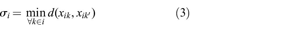
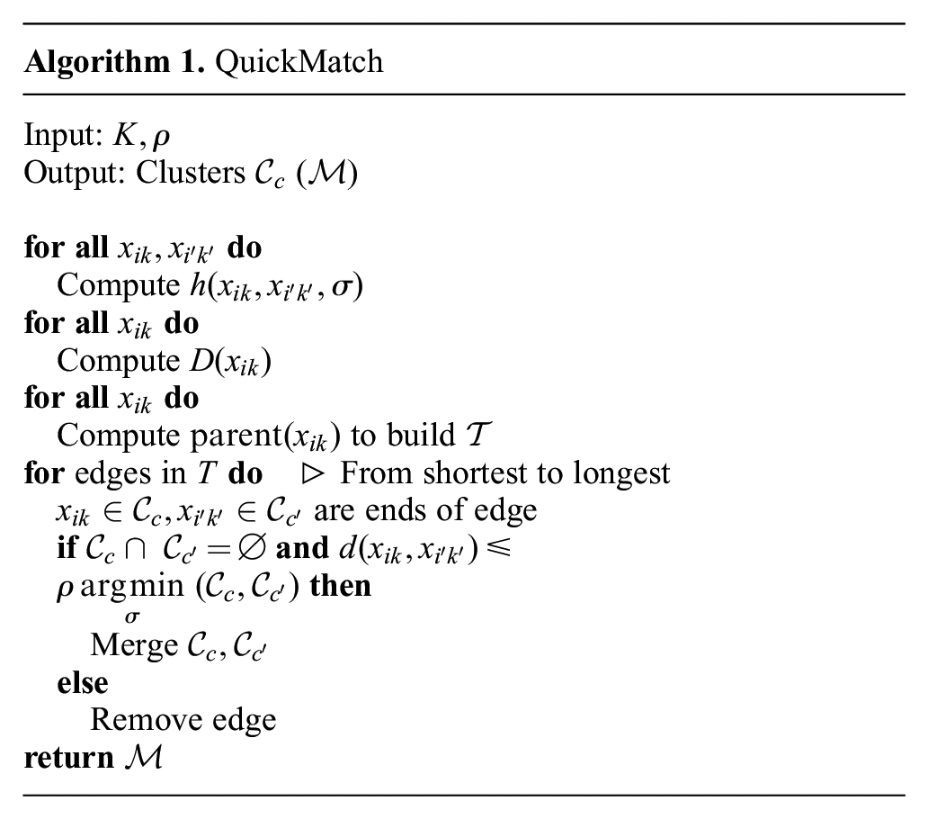
4.2. QuickMatch
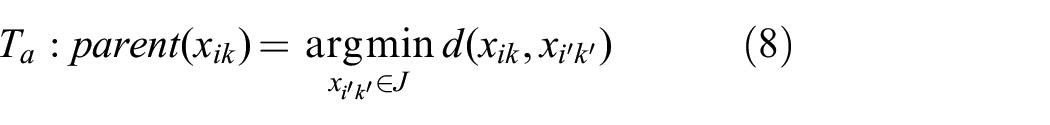
The QuickMatch algorithm begins by calculating the distance between all features (here we use the Euclidean distance). For each image, the minimum distance,
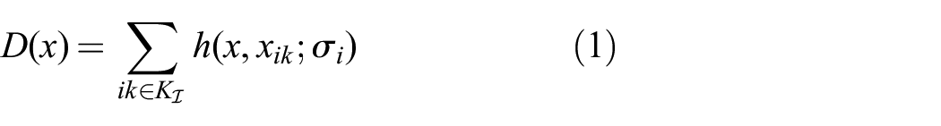
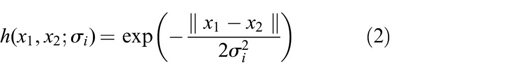
where h is a non-negative kernel function, and
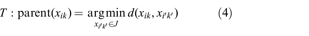

Edges are directed to parents along the gradient of feature density, and ultimately toward the center of the parent cluster or to another distant cluster. Once the tree has been constructed, edges are broken if either of two criteria are met (based on (C1)–(C3) above).
If parent and child groups have nodes from the same image (i.e.,
If the edge is larger than a user-defined threshold (
This method results in a forest of trees (
4.3. NetMatch
The centralized QuickMatch algorithm is limited in the number of features it can process, because a single computational unit must handle all of the processing. This limitation motivates distributing the computation across many computational nodes in order to increase the number of features considered. A similar situation occurs when the data is acquired and naturally distributed across different nodes. To this end, we introduce the NetMatch algorithm, which distributes features over a network of computational nodes such that each can run QuickMatch (or another equivalent algorithm) on only a subset of the feature space.
NetMatch follows three steps.
Each node transmits its computed features in such a way that one node receives all the features belonging to a given partition of the feature space; for instance, in a one-dimensional feature space, if a node is assigned the partition element
Each node performs QuickMatch independently on all received features in its assigned partition, stopping, by default, at the tree-building phase (i.e., without breaking the trees into clusters).
Computational nodes identify clusters falling near the edges of the partition. We refer to such clusters as contested.
If necessary, the contested clusters are transferred to other nodes for re-processing.
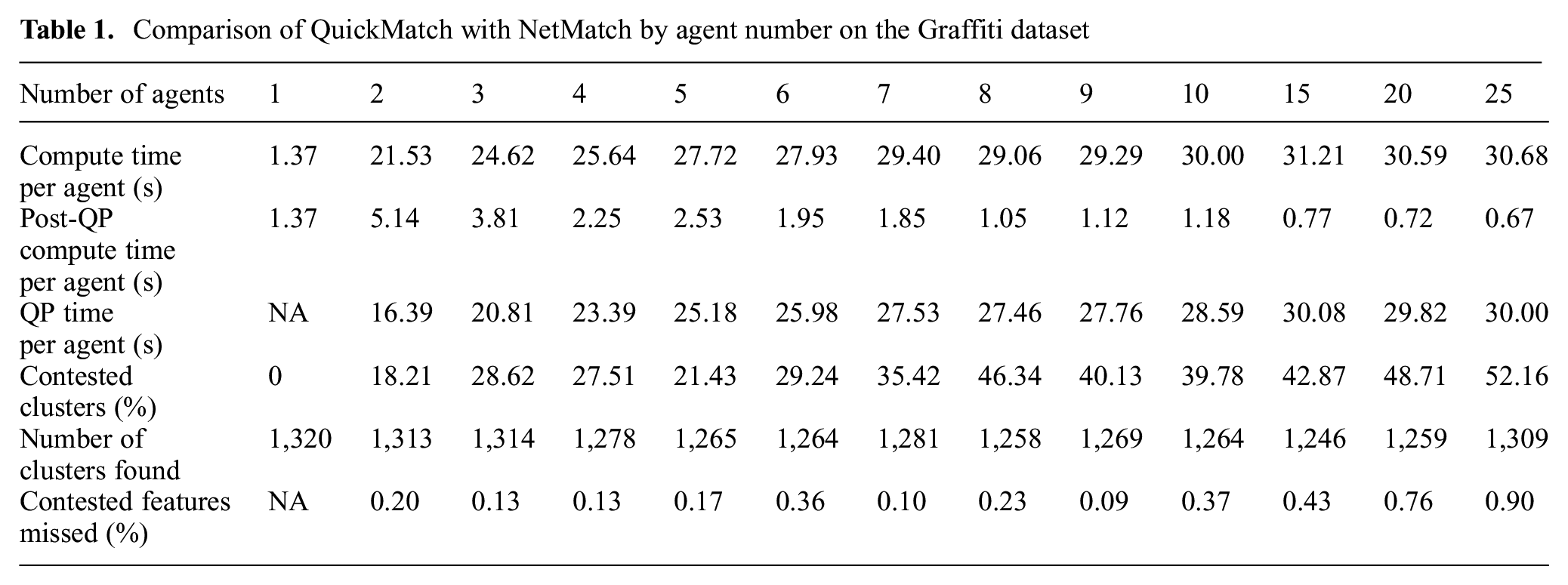
At a high level, each node needs to process only a subset of the entire dataset, and, more importantly, each point is typically transferred only once, without having to flood the entire network with the entire dataset (additional transmissions are required only for edge cases, which are usually a minority, see also Table 1 for a quantitative analysis in our experiments). We present below the details of each step.
Comparison of QuickMatch with NetMatch by agent number on the Graffiti dataset
4.3.1. Feature space partitioning
The goal of partitioning the feature space is to split the computation load of QuickMatch among m agents, ultimately allowing for more features to be matched, while approximately maintaining multi-image match quality. We begin by partitioning the feature space and send features to their nearest region center for processing. This initial partition can split a cluster between multiple regions. Finding and merging these split clusters will be the focus of the following sections.
We modify the labeling function presented in the preliminary section to denote the round being considered as

where the set of Voronoi seeds
As an alternative, in larger datasets, and in a more distributed setting, the choice of
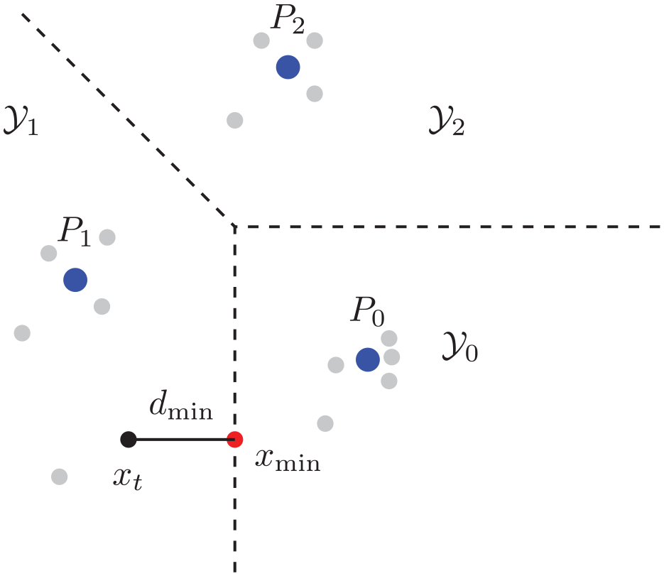
Illustration of Voronoi boundary distance problem.
4.3.2. Tree building
Once
Once the density is calculated, we build a tree

Similarly to the distinctiveness in QuickMatch, we now introduce an agent-specific distinctiveness metric, defined as
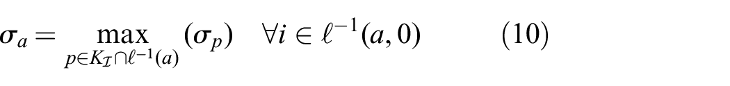
where

(in practice, p indexes the features in a given partition).
We next use
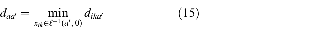
4.3.3. Partition boundary distance
To find the minimum distance between a feature and the boundaries that are generated by the Voronoi partition, we formulate the following problem: Consider a set of root nodes
Given the test feature node
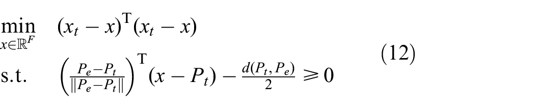
where

The boundary distance calculation could be simplified by considering only the partition boundary between the two nearest points in
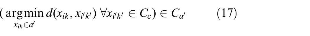
4.3.4. Contested feature re-assignment
Once we are able to determine the distance between a feature and the partition boundary, we can then determine the contested features in each region. These features are those that may require reassignment to another partition’s tree and are in danger of being mismatched due to the feature space partitions splitting their cluster. This contested set of features
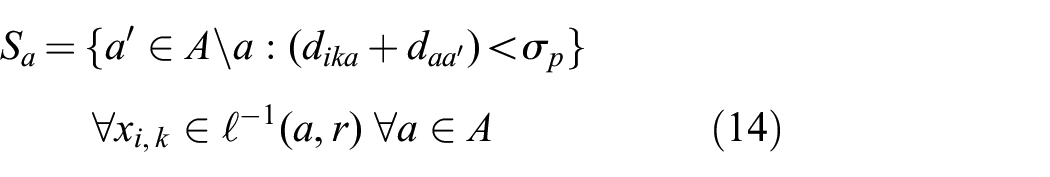
where
where
Intuitively, if the inequality in Equation (14) is true, there could be a feature in
Example of a comparison to determine whether a point is contested.
Once the contested features are determined, we break the agent tree into a forest of trees (clusters) in the same manner as QuickMatch, except that the distinctiveness
With the clusters formed, each agent then determines which clusters have contested points. Formally, we check if
Upon arrival at
where
Upon receiving a new cluster, an agent checks whether the cluster contains any points that it would consider contested. If so, the agent sends the whole cluster to the nearest agent of lower index, if one exists.
The final step in reassignment is to rerun the tree building and breaking routines from above to rebuild all of the clusters. Although this is computationally intensive, it does not require any further inter-agent communication. It was also found to perform better than only reassigning the contested points to the appropriate tree and breaking it accordingly. For a simple example of the complete NetMatch framework, see the Appendix.
5. Simulations
This article looks to compare primarily QuickMatch with NetMatch in simulation, and with off-the-shelf matching tools in an experimental setting. For a detailed comparison of the performance of QuickMatch with other state-of-the-art matching methods (particularly multi-image matching methods), see Tron et al. (2017).
We begin with an illustrative example of NetMatch on a synthetic two-dimensional dataset shown in Figures 3 and 8. Our test case includes 4 agents and 250 feature points. There are 25 underlying clusters, generated with random Gaussian distributions around 25 evenly spaced points, each with 10 sample features. Figure 3 illustrates many of the steps in Algorithm 2. Figure 3(a) shows the
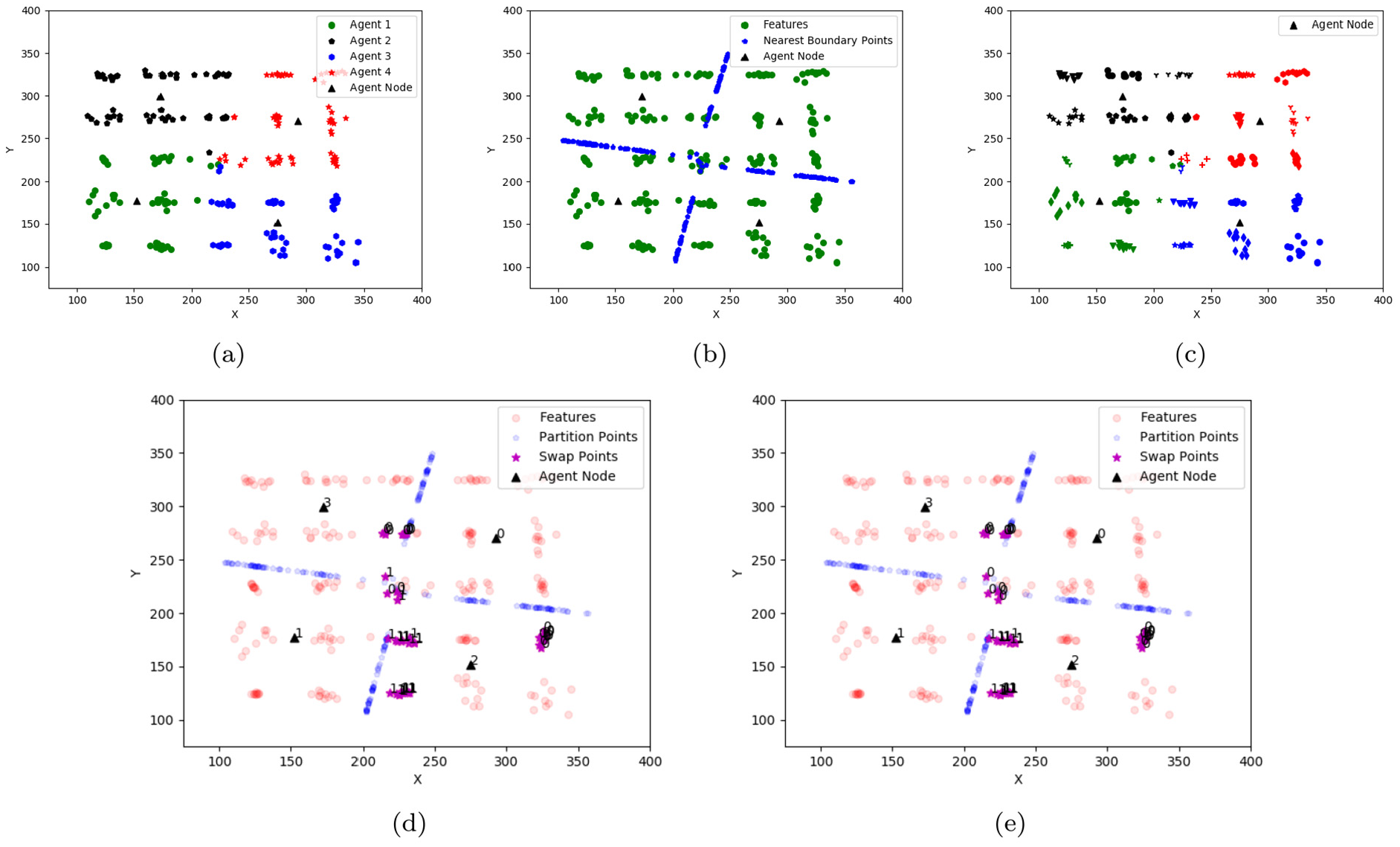
(a) Synthetic dataset features with naive k-means partition assignments. (b) Synthetic dataset with
The partition generated by the Voronoi seeds can be seen in Figure 3(b). Here, the
Figure 3(d) shows the clusters staged for initial agent switching. Each feature that is switched has a label of where it is being sent. Note that the central cluster has multiple labels, meaning even after the switch, the cluster will be segmented. In addition, note that whole clusters are staged for transfer, and that the contested region is very conservative, since clusters even somewhat far from the boundary are being swapped. After the agents are switched, the agents check whether the switched clusters are nearest to other contested points. Figure 3(e) shows the reassignment of the clusters after this check is performed. Note that after the first swap, the points in the central cluster are all moving toward
6. Experiments
6.1. Homography and localization
Homography is a projective transformation between two perspective images of a planar scene that can also be used to determine the relative pose of an object with respect to a given reference image. The study of homography and localization of images and objects is textbook material; however, a brief overview is provided below as this process is used to experimentally test QuickMatch’s performance. More information on both homography and object localization can be found in Hartley and Zisserman (2017) and Sankaranarayanan et al. (2008).
Given the image coordinates
Given
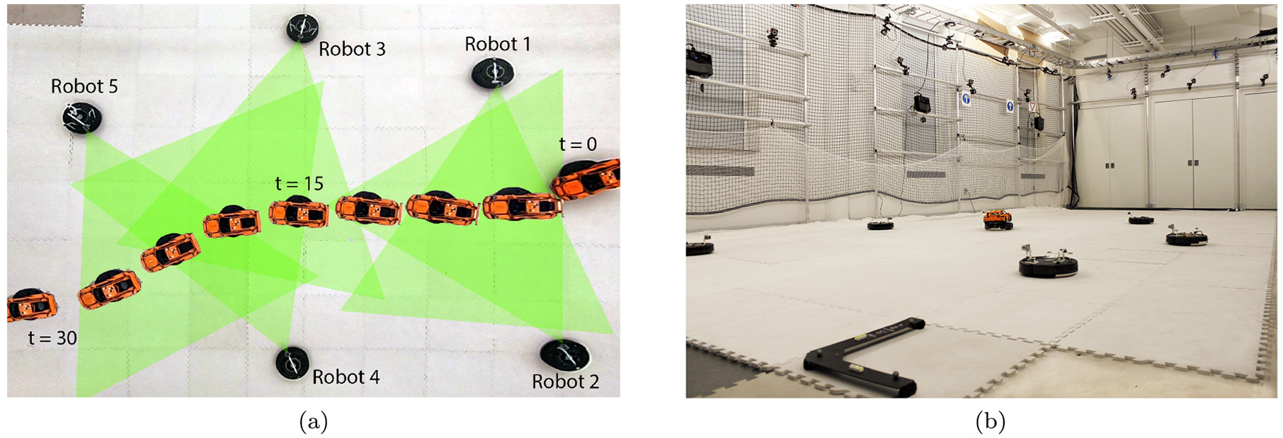
(a) Overhead view of experimental area with trajectory of the target object, position of the robots, and the approximate field of view for the camera network (shown in yellow). (b) Prospective view of experimental area with modified iRobot Create2 platform, target object, and overhead OptiTrack motion capture system.
As localization using homography is limited to approximately planar surfaces, multiple reference images (as used here) are required to identify different sides of an object. Second, despite the use of robust estimation (RANSAC), inaccurate matches are still possible, resulting in outlier measurements in distance and bearing. These inaccuracies are amplified by the sensitivity to errors in the estimate of the object’s height when calculating the target distance. To account for these errors, in practice, multiple measurements can be used to estimate each position, and then a filter can be used to smooth the target’s trajectory (e.g., a Kalman filter).
6.2. Experimental setup
The experiment consists of a team of five iRobot Create2 ground robots, each with a forward-facing camera, distributed throughout the experimental area shown in Figure 4. Each camera has a
7. Results
QuickMatch and NetMatch are evaluated in two ways: pure matching performance, and in the context of a target localization application. The algorithms are first compared with standard matching algorithms in the OpenCV Software Package (Bradski, 2000), BF, and FLANN. These algorithms use the Euclidean distance metric and a threshold match distance of 0.75 (Bradski, 2000; Lowe, 2004). Unlike QuickMatch and NetMatch, these algorithms cannot consider matches across more than two images but do have very low execution times.
QuickMatch is implemented in Python and takes 5.6 seconds to find matches between 6,254 SIFT features (from 115 images), whereas BF and FLANN are both implemented in C++, and both take approximately 0.05 seconds to find the matches between the reference image features, and the same 6,254 features. This time difference arises from two factors: the inherently slower run time of Python compared with C++ (Fourment and Gillings, 2008), and the extra comparisons done by QuickMatch to solve the entire multi-match problem. If BF and FLANN compared all images with all other images combinatorially (as QuickMatch implicitly does) their computation times would be
7.1. Precision versus recall
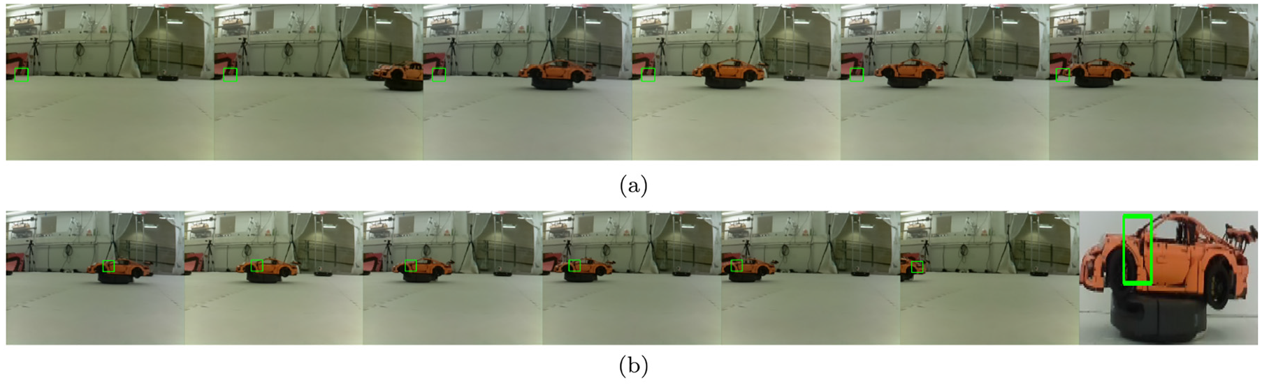
Although QuickMatch and NetMatch are slower, they outperform both BF and FLANN in the number of matches correctly found, and generally in terms of precision versus recall (PR) and precision–recall area under the curve (PRAUC), which are common metrics for evaluating matching algorithms (Ting, 2011). Figure 6(a) shows the precision (fraction of correctly matched images) versus recall (fraction of possible matches found) curves for QuickMatch, NetMatch, BF, and FLANN. For any recall level, QuickMatch and NetMatch maintain a higher precision level than either BF or FLANN. Both BF and FLANN have terminations before a recall of 0.9 because at that level of discrimination, they are unable to find any matches in the data. QuickMatch and NetMatch on the other hand are still able to find some matches. These curves are non-monotonic because mismatched features appear at a higher rate than correctly matched features at higher thresholds. Note that NetMatch has higher precision than QuickMatch at lower recall levels; we hypothesize that this is due to the fact that the introduction of partitions in the dataset reduces the interference between modes of different clusters in the feature density. At higher recalls, however, the partitioning limits its ability to find all of the possible matches. PRAUC is a threshold agnostic metric used for comparing overall performance of matching algorithms (Ting, 2011). In terms of PRAUC, QuickMatch achieves 0.64, whereas BF and FLANN reach 0.49 and 0.45, respectively. The overall increase in precision stems for QuickMatch’s ability to consider more instances of the reference object, by matching cycles of features across multiple images. It is therefore able to find the reference object not only more consistently, but with many more matched features. An example of these matches is shown in Figure 5.
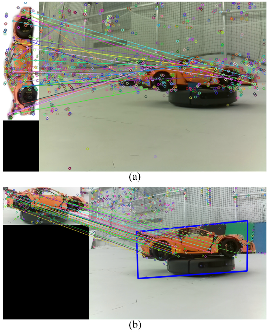
(a) Example image matches between the reference object image (left) and an experimental image (right): Circles represent features, and lines indicate matches. (b) Homography and localization of car with prospective transform of bounding box.
NetMatch and NetMatch Lite (see the note in Section 4.3.2 for details) are also evaluated on the same dataset as described previously. There are variables in NetMatch (random seed positions and number of agents) that result in a variable PR curve and therefore PRAUC. Figure 6(b) shows the effect of these variables on the PRAUC curve. First, note that as the number of computational agents increases, the PRAUC for NetMatch decreases slightly due to losses from split clusters. Second, note that the error bars (which represent one standard deviation of PRAUC over 10 trials with different partition seeds) show that the random seed position has a large effect on match quality. Specifically, a good partition can increase the PRAUC by as much as 13% in the best case and conversely a poor partition can decrease the PRAUC by as much as 11% compared with QuickMatch. The NetMatch Lite formulation (removing the contested feature swap) does not greatly reduce PRAUC (on average 3.5%) because many matches are still found (since the percentage of contested clusters is small). However, the match quality of NetMatch Lite is shown in the following to be much worse than NetMatch in an experimental setting (see Section 6). In addition, the standard deviations show that NetMatch Lite has a generally lower PRAUC and may be more susceptible to poor Voronoi seeding.
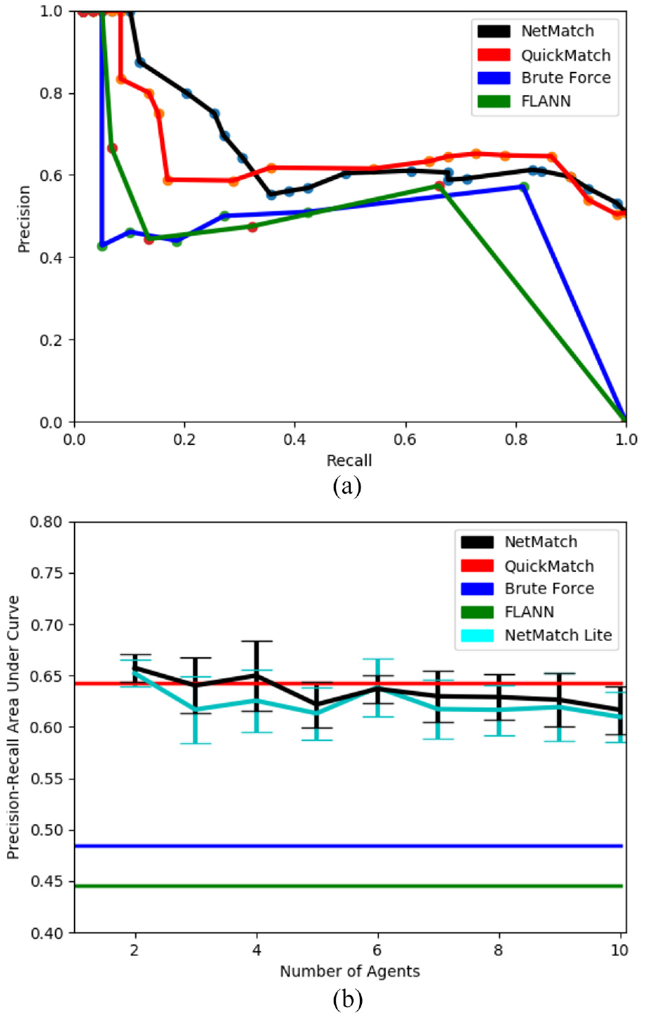
(a) Precision versus recall curves for the QuickMatch, NetMatch (
7.2. Homography and localization
In order to further demonstrate the utility of the algorithms, matches are used to localize a target object in relation to the camera network, and then estimate its global trajectory. This was done using all of the above algorithms with again an identical set of SIFT features. QuickMatch and NetMatch consider multi-image matches between the set of target images and the set of five robot images at each time step, whereas BF and FLANN consider matches between each target image and the robot image individually. Once feature matches are generated, RANSAC is used to estimate the homography matrix
These steps are performed using the match data from each of the above algorithms. Figure 7(a)–(e) show the results of the localization estimation for each algorithm. Red points are estimate target poses for each time step, blue points denote the ground truth measurements, black octagons are the camera positions, and the green regions are the one standard deviation error between all localization estimates at each time step. The localization error was found by taking the absolute distance between the estimated and ground-truth position at each time step. The average error is partly a factor of object height estimation, and the variance is indicative of the match quality. QuickMatch had an error of
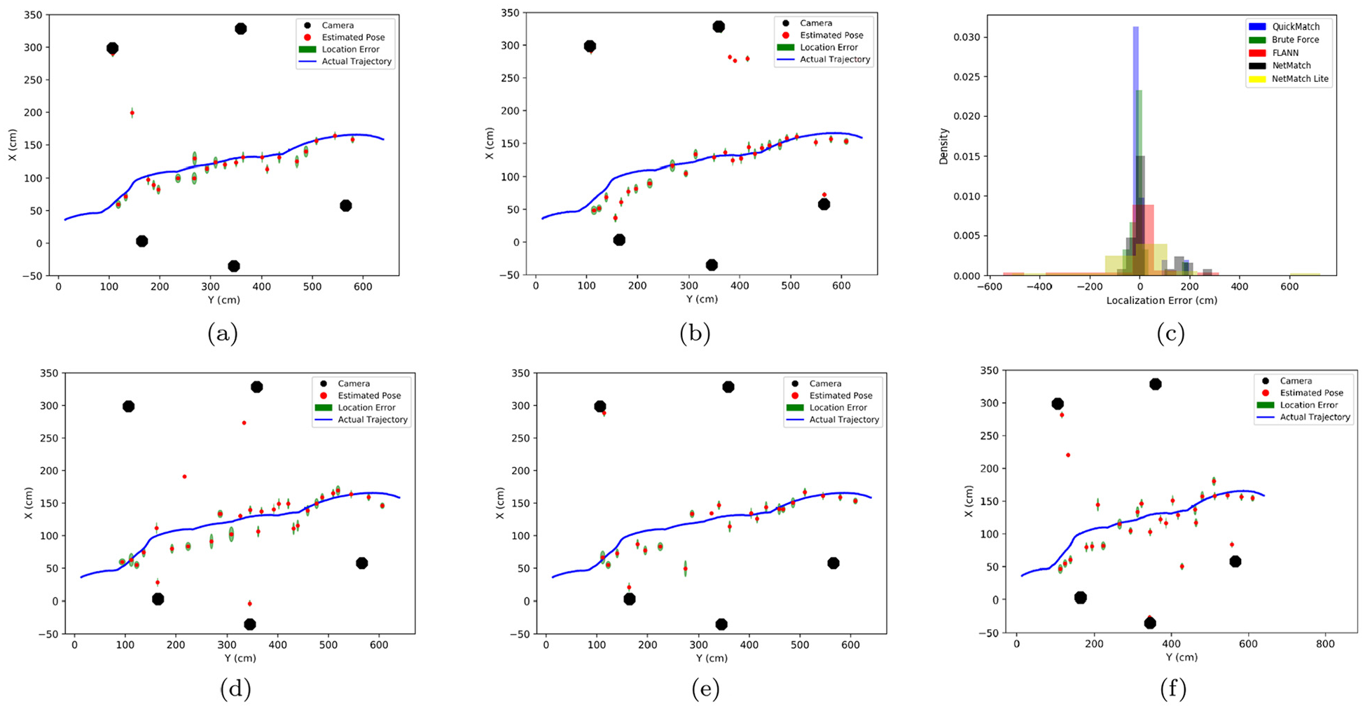
(a) QuickMatch trajectory estimates. (b) NetMatch trajectory estimates with six agents. (c) Histogram of estimate error for each algorithm. (d) FLANN trajectory estimates. (e) BruteForce trajectory estimates. (f) NetMatch Lite trajectory estimates.
7.3. Centralized versus distributed comparison
To test the difference between the distributed and centralized approaches, we look at how many clusters are split by naive partitions in the feature space to determine whether the distribution scheme above is even warranted. This test is performed on images from the Graffiti dataset (http://www.robots.ox.ac.uk/~vgg/data/data-aff.htm), in order to simulate realistic conditions where the ground truth is unknown. Given the clusters of features determined by QuickMatch,

where
With this quality metric, we can quantify the number of contested clusters in a given partition as
With this metric
To determine how many contested features, and hence split clusters, are missed by NetMatch, we calculate the following precision
where
The results of these tests are listed in Table 1. The first column in Table 1 lists the results of the centralized QuickMatch algorithm. Row five shows that as the number of agents increases, intuitively, the percentage of contested clusters also increases. At the same time, however, the post-QP computation time decreases as agent number decreases, because each agent has to work on considerably fewer features. The largest computational requirement in NetMatch is finding the boundary distances with the QP. The time reported for this is per-agent, however it is worth noting the implementation of this QP is sub-optimal. In the QP formulation, we consider each partition individually, meaning we solve m QPs for each feature. In the future, we plan to reduce this to combining all of the constraints to solve a single QP and this is a focus of future work. One key aspect of NetMatch to note is that it finds around 99% of all contested points, meaning it is very good at finding split clusters. One interesting result of NetMatch is that it matches the features into fewer, larger clusters owing to the use of its finite density kernel. This is a counter-intuitive result and will be a subject of future study for this algorithm.
The final clustering results from the synthetic dataset in the Simulation section are shown in Figure 8. Figure 8(a) shows the result of the centralized QuickMatch algorithm run on the synthetic data, whereas Figure 8(b) shows the final result from NetMatch. Note that many of the features from the higher index agents have been shifted to the lower index agents, but ultimately each cluster has features belonging to only one agent. Ultimately both algorithms are able to cluster all of the features correctly.
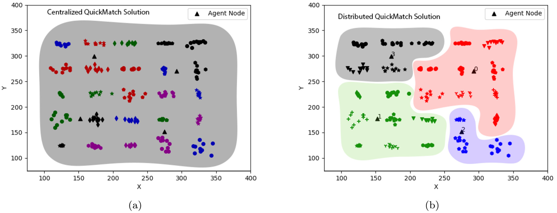
(a) Clustering result from the centralized QuickMatch algorithm on the synthetic dataset. Feature color denotes cluster membership. (b) Clustering result from the NetMatch algorithm on the synthetic dataset. Feature color denotes agent membership.
7.4. Feature discovery
The QuickMatch and NetMatch algorithms implicitly discovers common features among images by creating clusters of similar features. These clusters correspond to specific locations in the universe, and therefore can be used to find both targets and landmarks across images. Landmarks, although not used in this article, are points that occur commonly across all images (except when occluded), and are useful for multi-agent localization tasks. In the experimental images collected, landmarks were the clusters with the largest number of features, because many of this images did not contain the target object. An example landmark cluster is shown in Figure 9(a). Features belonging to the target object are generally smaller than the landmark clusters, but can still be extracted, and show key features of the target. Figure 9(b) shows one such cluster, which is the front hood of the car model. Feature discovery is one attribute of QuickMatch and NetMatch that does not exist in either BF or FLANN and can be useful for discerning what features are most descriptive of images from the network.
(a) Landmark feature cluster. (b) Target feature cluster.
8. Conclusion
This article has highlighted the utility of QuickMatch multi-image matching for object matching and presented the NetMatch algorithm. QuickMatch was able to find many more object feature matches than standard methods by considering matches across all images, not just pairwise matches. The presented experiment has tested the QuickMatch algorithm in an experimental setting with realistic conditions, and shown that multi-image matching is superior to standard methods at matching the reference object (even as it enters and exits images across the entire camera network). QuickMatch has also been tested with a target object localization and again outperforms both the BF and FLANN algorithms. Beyond testing QuickMatch, we have demonstrated the capabilities of NetMatch as a distributed solution to the same problem. We have also demonstrated QuickMatch’s feature discovery ability by showing a characteristic landmark and target feature cluster from the test images. This approach is the precursor to an online and decentralized approach. Our future work will focus on the online version of object discovery and localization and multi-camera homography. We also plan to decrease NetMatch’s QP implementation computation time. Overall, QuickMatch has been shown to be a versatile multi-feature matching algorithm that outperforms standard pairwise matching algorithms, and NetMatch offers an avenue for the QuickMatch framework to handle a large volume of features with minimal inter-agent communication.
Footnotes
Appendix
Funding
The author(s) disclosed receipt of the following financial support for the research, authorship, and/or publication of this article: This work was supported by the National Science Foundation (Grant Nos. NRI-1734454 and IIS-1717656).
Supplemental material
Supplemental material for this article is available online.