






Abstract
A holistic semantic scene understanding exploiting all available sensor modalities is a core capability to master self-driving in complex everyday traffic. To this end, we present the SemanticKITTI dataset that provides point-wise semantic annotations of Velodyne HDL-64E point clouds of the KITTI Odometry Benchmark. Together with the data, we also published three benchmark tasks for semantic scene understanding covering different aspects of semantic scene understanding: (1) semantic segmentation for point-wise classification using single or multiple point clouds as input; (2) semantic scene completion for predictive reasoning on the semantics and occluded regions; and (3) panoptic segmentation combining point-wise classification and assigning individual instance identities to separate objects of the same class. In this article, we provide details on our dataset showing an unprecedented number of fully annotated point cloud sequences, more information on our labeling process to efficiently annotate such a vast amount of point clouds, and lessons learned in this process. The dataset and resources are available at http://www.semantic-kitti.org.
1. Introduction
Since autonomous vehicles successfully completed the driving tasks at the DARPA Urban Challenge (Montemerlo et al., 2008; Urmson et al., 2008), the prospect of fully autonomous cars led to founding of many startups pursuing the endeavor of creating always attentive robotic cars that prevent and avoid traffic fatalities occurring today due to human error. After the Urban Challenge, many expected and predicted that cars capable of driving fully autonomously in dense urban traffic would be already reality by today. However, solving the driving task in real-world environments with many non-compliant traffic participants that might violate rules and with the complexity of sometimes contradictory signage is a stupendous endeavor.
Perception is a centerpiece of every intelligent robotic system to handle the complexities of operating in semi-structured and natural environments. In particular, self-driving cars rely on robust and accurate perception systems that allow them to perform safe and efficient driving maneuvers. For a holistic semantic scene understanding, they need to perceive obstacles, identify other traffic participants, but also reason about functional street surface types, e.g., parking areas, lanes, and sidewalks.
Recent progress in perception using images, but also LiDAR sensors, is driven by advances in deep learning enabling end-to-end trainable perception systems without the need to hand-craft features (LeCun et al., 2015). Training deep neural networks with millions of parameters was mainly enabled by two essential developments: (1) the possibility to repurpose graphics processing units (GPUs) from producing pixels on a computer screen to compute matrix products in a highly parallel fashion; and (2) the availability of large-scale labeled datasets, such as ImageNet (Deng et al., 2009), that enabled training networks without over-fitting to the training data.
Real-world datasets play an important role in the aforementioned endeavor to attain fully autonomous cars, as they provide realistic data on the one hand, but also allow us to measure progress towards our goal on the other hand. Datasets, such as Cityscapes (Cordts et al., 2016) and Mapillary Vistas (Neuhold et al., 2017), enable fine-grained perception tasks to be investigated, such as semantic segmentation (Everingham et al., 2010) providing classes for each pixel, but also panoptic segmentation (Kirillov et al., 2019), which additionally distinguishes between individual instances of the same class. More specifically, semantic segmentation distinguishes between classes but assigns different objects the same label, e.g., different cars cannot be distinguished. Panoptic segmentation differentiates additionally between objects leading to clear object boundaries or instances. However, panoptic segmentation requires instance IDs only for so-called thing classes, which have clear boundaries, such as cars, pedestrians, and bicyclists. The remaining classes are called stuff classes and do not get an instance ID assigned, such as vegetation, road, or sidewalks.
We present a dataset based on the KITTI Vision Benchmark (Geiger et al., 2013, 2012) that enables the investigation of semantic segmentation and panoptic segmentation using point clouds from an automotive LiDAR sensor. To this end, we annotated all 22 sequences of odometry evaluation of the KITTI Vision Benchmark (Geiger et al., 2013, 2012) consisting of over 43,000 scans using 28 classes. We labeled each point of the point cloud such that corresponding instances of object classes get temporally consistent instance annotations. In addition, we use the annotated sequential data and accurate poses to generate a real-world dataset for semantic scene completion, where an algorithm needs to provide class labels for voxels, but also predict the completed scene which is not visible in the given input voxelized scene. As commonly done with other datasets (Cordts et al., 2016; Lin et al., 2014; Neuhold et al., 2017), the test set labels are not published to ensure an unbiased and fair evaluation. We use CodaLab Competitions (see https://competitions.codalab.org/ for more information) that provides a platform to upload results for a hidden test set, which are then evaluated using a custom evaluation script on cloud-based evaluation servers without revealing the testset annotations.
This article complements our other papers (Behley et al., 2019, 2020), because it focuses on the dataset itself. We provide more details on the annotation process and statistics about the automatic instance extraction process. We, furthermore, discuss lessons learned in the process of annotating a large-scale dataset and maintaining an online evaluation with a hidden test set. Thus, the article provides additional information, compared with the more task-oriented papers, and we refer to these for more details on the tasks, baselines, and evaluation metrics for semantic segmentation and scene completion (Behley et al., 2019) and panoptic segmentation (Behley et al., 2020).
2. Related work
In the following, we focus on datasets providing LiDAR point clouds and, in particular, on datasets that provide annotations for perception tasks, such as object detection, semantic segmentation, or panoptic segmentation.
The seminal KITTI Vision Benchmark (Geiger et al., 2012) aimed at providing a collection of different benchmark tasks to evaluate perception algorithms for autonomous driving. It made a vast collection of data (Geiger et al., 2013) available that was recorded with a sensor suite commonly used by self-driving cars including a stereo camera, a Velodyne HDL-64E LiDAR, and an inertial navigation system (INS) to generate ground-truth data for pose information. The provided benchmarks propelled research in the areas of motion estimation and traffic scene perception and enabled reproducible experiments with standardized metrics.
Since then, only a few LiDAR datasets have been recently published that are recorded either with a terrestrial laser scanner (TLS), such as the Semantic3d dataset (Hackel et al., 2017), or using automotive LiDARs, such as the Paris-Lille-3D dataset (Roynard et al., 2018).
Recently, several major self-driving car ventures released datasets providing camera images in addition to LiDAR point clouds, including Waymo (Sun et al., 2020), Lyft (Kesten et al., 2019), Audi (Geyer et al., 2020), Argo (Chang et al., 2019), Honda (Patil et al., 2019), and Motional (Caesar et al., 2020). Although all these datasets provide instance annotations using bounding boxes, only a few datasets provide point-wise semantic annotation (Geyer et al., 2020; PandaSet, 2020).
The A2D2 dataset (Geyer et al., 2020) provides annotations for semantic segmentation of images that can be used to obtain point-wise labels by projecting LiDAR points into the images and using the associated semantic class from the pixel-level annotation. However, this projection will never cover all LiDAR points owing to the sensor placement and the resulting different view point. The very recently published PandaSet (PandaSet, 2020) provides point-wise annotations of LiDAR point clouds with 42 classes focusing on objects on the road, such as traffic participants, barriers, and cones, and more fine-grained distinction between different vehicle types compared with our annotation. SemanticPOSS (Pan et al., 2020) also provides semantic annotation of point clouds with a focus on scenes with pedestrians captured in a campus environment. The classes are compatible with our classes and the authors provided labels in the same format as our annotation data. Pan et al. (2020) used our annotation tool presented in Section 3.1, but used tracking information to extract instances. NuScenes (Caesar et al., 2020) also recently added annotations for LiDAR point clouds with more diverse categories for different traffic participants. Together with the bounding box annotations, this dataset can also be used for panoptic segmentation. Owing to the large number of different scenes, it provides a highly diverse set of situations.
Table 1 provides an overview of the aforementioned datasets and their characteristics. Other automotive datasets might provide more diversity in terms of cities or number of different scenes. However, our dataset is the only dataset that combines point-wise semantic annotations directly made in sequences of three-dimensional point clouds with temporally consistent instance annotations for both non-moving and moving traffic participants.
Overview of other point cloud datasets with bounding box (top) and semantic annotations (bottom).
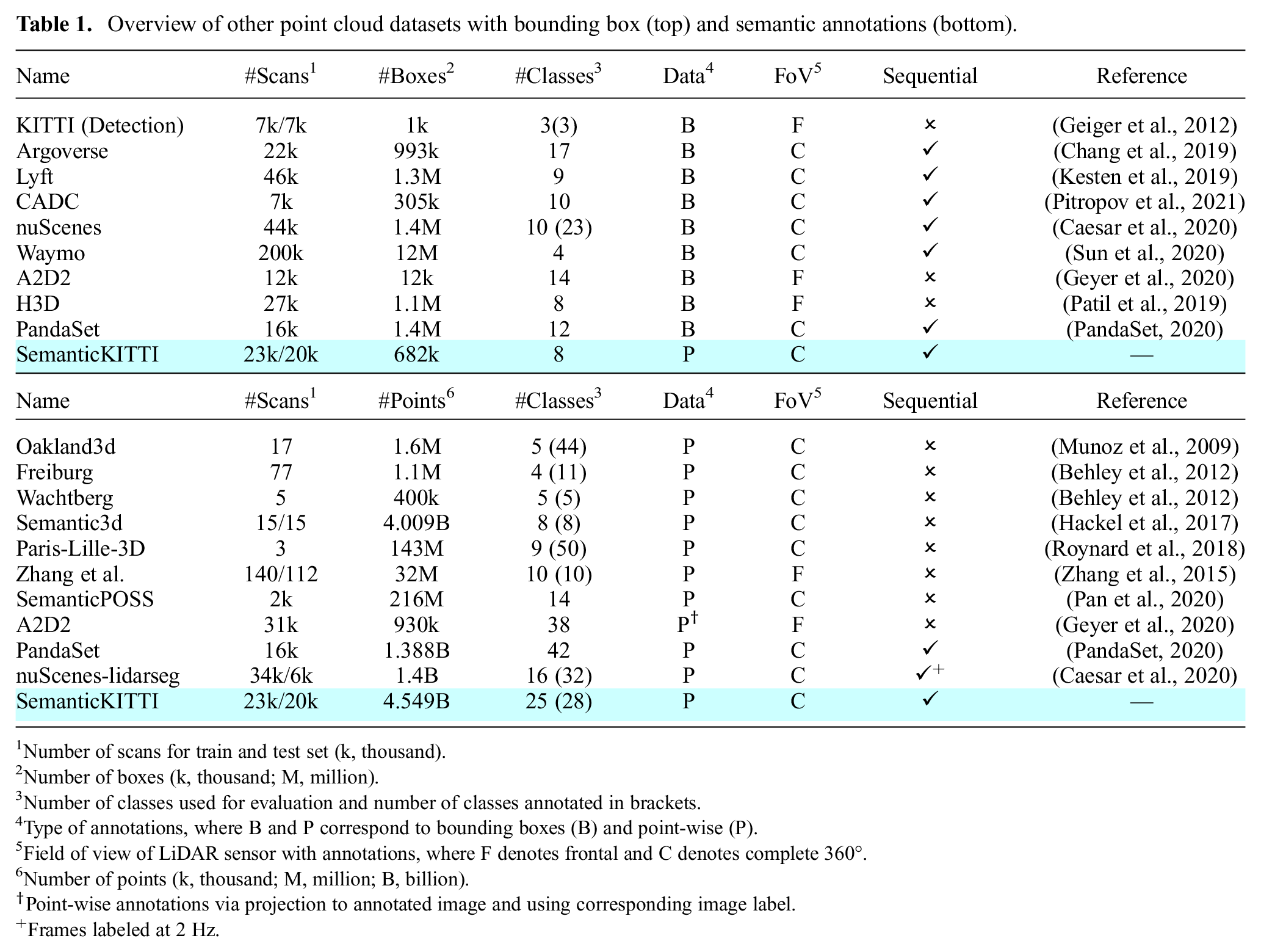
Number of scans for train and test set (k, thousand).
Number of boxes (k, thousand; M, million).
Number of classes used for evaluation and number of classes annotated in brackets.
Type of annotations, where B and P correspond to bounding boxes (B) and point-wise (P).
Field of view of LiDAR sensor with annotations, where F denotes frontal and C denotes complete 360°.
Number of points (k, thousand; M, million; B, billion).
Point-wise annotations via projection to annotated image and using corresponding image label.
Frames labeled at 2 Hz.
3. Dataset
Our dataset provides point-wise semantic annotations for the odometry sequences of the KITTI Vision Benchmark Suite (Geiger et al., 2013), which was the first large-scale dataset providing data recorded with a platform equipped with sensors commonly used on self-driving cars since the DARPA Urban Challenge (Montemerlo et al., 2008). The recording vehicle was equipped with a stereo camera covering the frontal field of view and a rotating 3D LiDAR sensor, the Velodyne HDL-64E S2, covering the full
In the case of the odometry benchmark, 1 we use the data provided that uses point clouds of a single turn of the LiDAR sensor which are compensated for sensor motion, i.e., individual points in the point cloud are transformed to account for the movement of the sensor during a single turn of the rotating LiDAR sensor.
The odometry dataset comprises 22 sequences: 11 training sequences (sequences 00–10) with ground-truth poses and 11 testing sequences (sequences 11–21) without pose information for which an odometry approach should estimate the poses. The pose error is only locally evaluated and therefore the provided poses are not closed loop or optimized to give globally consistent poses, such that already visited areas would be consistently mapped and old and new point cloud observations of the same place would be aligned properly.
3.1. Point cloud annotation
Our primary objective is to generate a consistent, accurate labeling of the sequential point clouds. It is essential to have consistent and closed-loop poses to facilitate the consistent annotation by accumulating point clouds from multiple scans. Figure 1 shows some qualitative examples of the provided annotations and the achieved fidelity of the point cloud annotations.
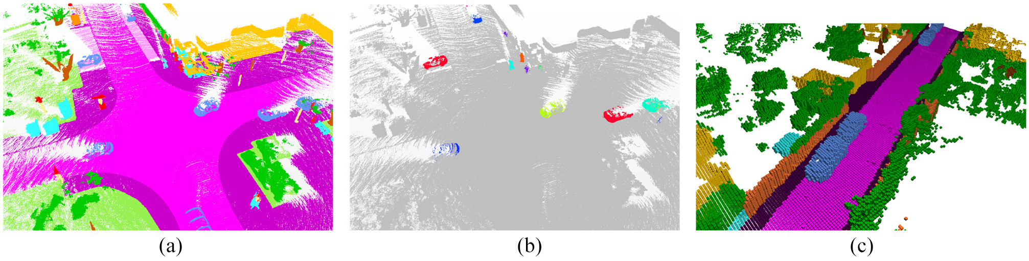
Qualitative examples of the provided annotations from sequence 08. In (a) we show the semantic annotation and (b) shows the corresponding instance annotation of 50 aggregated scans. We also provide input (not shown) and target voxel grids aggregated from multiple scans for the semantic scene completion task as shown in (c).
3.1.1. Pre-processing
To estimate globally consistent poses, we employed our surfel-based simultaneous localization and mapping (SLAM) approach (Behley and Stachniss, 2018). Our mapping approach finds heuristically loop closures using a map-based criterion and performs then pose graph optimization using loop closure constraints to obtain globally consistent poses. For sequences 02 and 07, where the automatic loop closure detection missed loop closures, we manually inserted loop closure constraints to ensure consistent mapping results.
3.1.2. Point cloud annotation
Using the estimated poses, we split the complete trajectory of a sequence into tiles of a given size (we used
Our point cloud labeling graphical user interface provides different filtering methods to facilitate labeling, such as hiding points from a specific class or above/below an adjustable plane. The filtering allows us to accurately label points even in complex situations with overhanging vegetation that cover the view onto parts of the point cloud. Figure 2 shows our labeling application with a challenging situation, where we have a bridge over a street and foliage from overhanging trees.
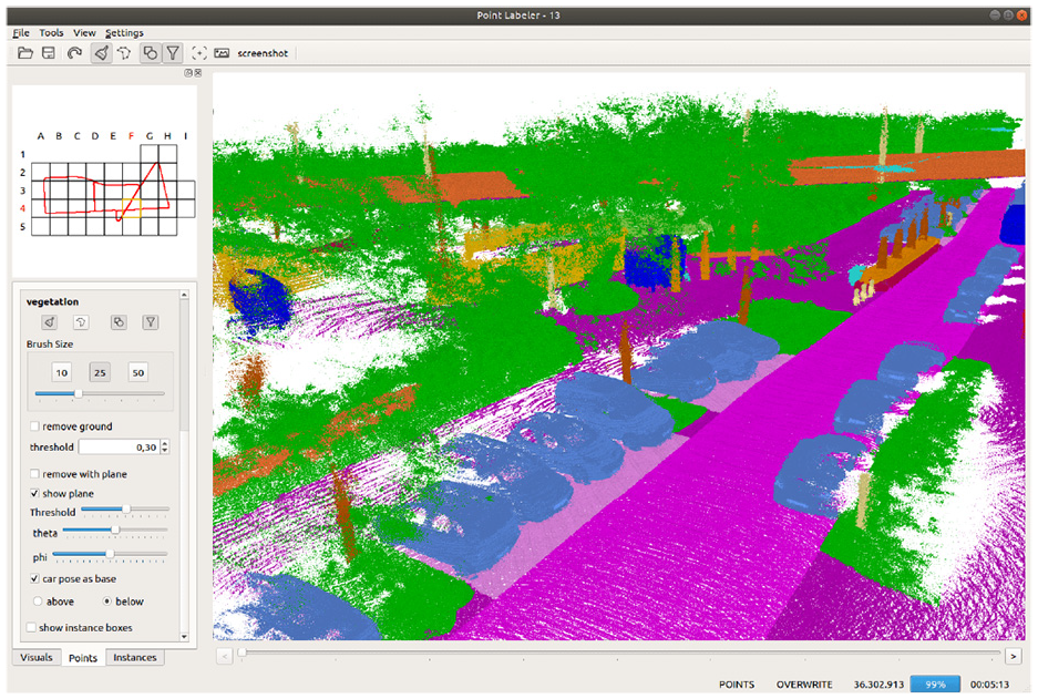
Our point cloud labeling application for sequential point clouds that we provide together with the dataset.
We provide two tools for annotating the point cloud: (1) a brush, which labels all points in a circular region around the current mouse position and (2) a polygon, which labels all points inside the polygon area specified by setting the polygon corners. Both operations happen on the projected points, where we check the projected three-dimensional point in the image plane for inclusion in the brushed or selected area. Thus, labeling of the point cloud is viewpoint dependent and requires a viewpoint to be found that does not affect points that lie in the line of sight. Here, the aforementioned filtering tools allow such points or simply all already annotated points to be filtered.
3.1.3. Class annotation
Following best practices for dataset labeling, we compiled a labeling instruction based on Mapillary’s instructions (Neuhold et al., 2017) and provided instruction videos on how to label certain objects such as cars and bicycles standing near a wall to our annotators.
Compared with image-based annotation, the annotation process with point clouds is more involved owing to the aforementioned view dependency. The annotator often needs to change the viewpoint to find a perspective where an annotation is possible without annotating unwanted or already labeled points. An annotator needs on average
We provided feedback to the annotators to improve the quality and accuracy of labels. Furthermore, we also checked the labels in a second pass and inspected already labeled point clouds. During this check, inconsistencies were corrected and missing labels were added.
To ensure consistent annotations, a single annotator performed the verification of all sequences. Table 2 lists the fraction of points for each sequence, which we relabeled in the verification process. Thus, relabeling percentages are low for sequences mainly handled by this person, i.e., sequences 00, 09, and 13. The number of relabeled points with the remaining sequences show the range of agreement between our annotators ranging from 2% up to 15%. The rather large spread compared with other image datasets (Cordts et al., 2016; Gupta et al., 2019; Lin et al., 2014) can be attributed to having annotators from different backgrounds, who had not previously annotated point clouds. Thus, we and the annotators had to learn and refine the process while creating the annotations.
Relabeling and instance correction statistics for training (top) and test data (bottom).
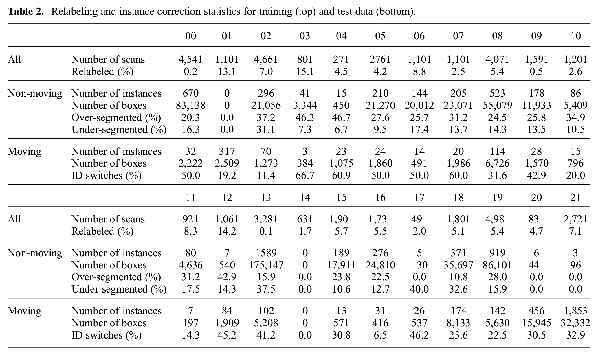
Figure 3 shows examples of corrected labels during the verification process. Usually, we refined the boundaries of the road/sidewalk (e.g., curbs are always labeled as sidewalk), added details that where missed (e.g., tree trunks, guard rails, etc.), or refined the boundaries between different classes (e.g., building and sidewalk, car and road, etc.).

Examples of correction during the verification process (top shows before validation and bottom after the validation). Here, we show (a) refined road boundaries, (b) added details (guard rail in the vegetation), and (c) refined boundaries between classes.
3.1.4. Instance annotation
For non-moving objects, we first cluster all points for each class using a fast grid-based segmentation approach (Behley et al., 2013). We use the aforementioned tiles to build a two-dimensional grid with cell size
For moving objects, we cluster each scan individually using a distance-based clustering as this provided more reliable results and it can be used to associate instances between consecutive scans using the same principle. First, we search for each point its radius neighbors within
The described clustering leads inevitably to over- and under-segmentation, but also to wrong or missing associations between consecutive timestamps. We correct these issues manually using our point labeling tool, which allows us to create, join, and split instances.
Table 2 shows the fraction of over- and under-segmented non-moving objects that where manually corrected. For determining over- and under-segmented segments, we inspect all segments after the correction and compared the instance IDs before and after the correction of the corresponding segments. If we find multiple instance IDs in the segment before the correction, we record an over-segmentation. If we find that the segment before the correction is larger then the segment after the correction, we record this segment as an under-segmentation.
Note that we can exploit the pose information of the LiDAR sensor for non-moving objects, since we can cluster points based on their global coordinates. Only this allows us to inspect all 682,000 bounding boxes, because a large part of instances originate from non-moving objects.
However, Table 2 also reveals that 30–50% of all segments were affected by over- and under-segmentation, which had to be manually corrected. Our axis-aligned grid often under-segmented nearby parked cars in non-axis aligned directions and over-segmented cars that were farther away owing to the point distance.
For moving objects, we report in Table 2 the fraction of object trajectories that have at least once a different instance ID in the automatically extracted instances. These data association errors were mainly caused by occlusions or by cars moving in the same direction with a small gap. Using here a tracking-based data association, which accounts for the object motion, would have resolved many of these issues.
3.2. Class and instance distribution
Overall, we annotated over 500 tiles resulting in the class distribution shown in Figure 4. In addition to traffic participants, such as car, truck, bicyclist, motorcyclist, we also included more functional ground classes relevant for autonomous driving, such as sidewalk and parking areas. Note that we also differentiate for potentially moving classes between non-moving, i.e., the object did not move while observing it, and moving objects, i.e., the object moved at least for a single frame while the sensor observed it. In total, we distinguish between 28 classes including the moving and non-moving classes.
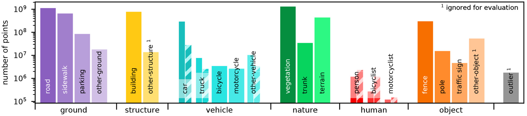
Class-wise distribution over the complete dataset. For the potentially moving classes car, truck, other-vehicle, person, bicyclist, motorcyclist, we furthermore distinguish between non-moving (solid) and moving instances (dashed bars).
Note that we label points belonging to a bicycle or a motorcycle also as bicyclist or motorcyclist, when the vehicle has a rider. This simplification was needed, because persons on a bicycle or motorcycle cannot be separated reliably and accurately from the vehicle. Owing to the sparser resolution of the point clouds compared with images, we preferred to label only the complete objects.
Naturally, road, vegetation, and building points are by far the most frequently occurring classes. Motorcyclist is a class with only few examples present in the data.
The class car is by far the most often occurring traffic participant, which can be also seen in the object count depicted in Figure 5 . We show in the upper part of Figure 5 the sequence-wise counts of instance annotations, i.e., we count each object only once even if it is seen multiple times by the sensor. The lower part of the figure shows the accumulated scan-wise counts of instances, where we count the instances without considering the temporally consistent instance ID.
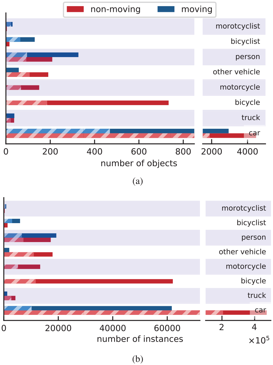
Instance-wise statistics over individual (a) object occurrences and (b) total count of bounding boxes or instances. Dashed bars show the proportion of objects in the training and validation data (sequences 00–10).
3.3. Dataset organization and format
We tried to keep the data organization as close as possible to the original KITTI Vision Benchmark. Thus, we use the same format for our pose files and a similar binary format corresponding to the point cloud format of KITTI. Pose information is given in the coordinate frame of the camera, therefore the calibration data of each sequence provided by the KITTI odometry benchmark is needed to correctly transform the point clouds.
We added the folder labels containing for each point cloud a binary label file. Corresponding to each point, this file contains a 32-bit unsigned integer, where the upper 16 bits contain the instance ID and the lower 16 bits contain the class ID. Here, a value of zero corresponds to no instance assigned to the corresponding point and a zero label corresponds to an unlabeled point.
The folder voxels contains the voxelized point clouds, the voxel-wise labels, the invalid voxels, and the occluded voxels. Here, we opted for reducing the size of the data by using only bit flags to encode 8 voxels inside a single byte. Labels are represented by a 16-bit integer and we do not distinguish between different instances.
3.4. Benchmark competitions and development kit
Together with the data, we also provide competitions on CodaLab Competitions that allow evaluating approaches on a hidden test set, i.e., part of the data for which we do not provide annotations. We use the original test sequences 11–21 of the odometry benchmark, because we do not want to interfere with the original benchmark which could exploit the provided labels to get better results on the original odometry benchmark. The large test set might furthermore incentivize the development of fast approaches to process the large number of scans.
We currently provide competitions for semantic segmentation, semantic scene completion, and panoptic segmentation. More information regarding the baselines and metrics are provided in the corresponding papers (Behley et al., 2019, 2020).
Together with the dataset, we also published a development kit 2 implemented in Python that provides methods to read the data and contains all evaluation scripts used in the aforementioned competitions. We furthermore provide tools to visualize the point clouds and the voxel grids.
4. Lessons learned
In the process of labeling around 43,000 point clouds with a team of nine annotators, we learned quite a bit about managing the annotation process, but also encountered pitfalls. From these experiences, we want to share some insights that might help others to organize annotating data at such scale and avoid some failures.
We relied on university students from computing related, but also unrelated fields. Accurate and still efficient annotators are hard to find and we had a selection process or casting, where we let the prospective annotators use our point cloud annotation application and could directly see how they performed in the session. During this process, we recognized that point cloud annotation is quite challenging and that even annotators that are comfortable with labeling images had big problems to navigate and transfer this knowledge to the annotation of point clouds. Thus, annotator screening turned out to be a mandatory first step to achieve good results.
However, we learned most about the problems and challenges by labeling ourselves. This also helps to rectify the expectations and helps in the selection of the targeted classes. We found early on that labeling lane markings would have increased the time per tile to much, such that we decided not to include these in our labeling effort.
Next, we had to invest additional time in training and correcting the annotators continuously to ensure sufficient quality of the provided annotations. Only this ensured a high quality of the resulting annotations and a speed up in the process. Interestingly, all annotators improved during this process substantially and could adopt our suggestions to label more efficiently. As we also used our own tools, we could develop and refine our annotation application over time and introduce new ways of filtering points, which also decreased the time needed to label a point cloud. Initially, we relied mostly on a height-based ground removal, which was not sufficient to consistently remove ground points. Adding a plane-based removal, where the annotator could set the angles and the threshold along the
Nevertheless, some of our early attempts to speed up the process by using pre-trained and fine-tuned image segmentation methods did not succeed. First, we aimed at having consistent labels for the aggregated point cloud and therefore the projection of single image labels to the point cloud needed to be aggregated using a point-wise majority vote. Second, the view point differences between the LiDAR sensor and the camera led to occlusions that could not always be resolved by aggregating multiple projected image labels, because one had only a frontal view available. Third, the misalignment between camera and LiDAR caused by pixel shifts or simply the rotation of the LiDAR resulted in “bleeding” of semantic labels into background regions or inconsistent labels on objects where parts of nearby classes got projected onto. Surprisingly, correction of these boundary issues took nearly as much time as labeling the whole tile from scratch. In addition, our impression was also that the transferred labels biased the annotations in being “good enough,” but being actually inferior to a labeling from scratch, because error or small problems with the projection of annotations are hardly visible.
5. Conclusion
SemanticKITTI provides point-wise semantic and instance annotations for all sequences of the KITTI odometry benchmark. At the time of writing, it is still the largest dataset that provides such annotations for point cloud sequences. Based on these annotation, we provide benchmarks for semantic segmentation and semantic scene completion (Behley et al., 2019). We added recently panoptic segmentation joining semantic and instance segmentation to the set of benchmarks (Behley et al., 2020). Furthermore, we plan to extend the set of benchmarks with additional tasks.
In addition to these benchmarks, we also see already adoption of the data for other domains benefiting from semantics, such as semantic SLAM (Chen et al., 2019; Gan et al., 2020), LiDAR-based localization (Yan et al., 2019), and loop closure detection (Chen et al., 2020). Moreover, domain adaptation (Jaritz et al., 2020; Langer et al., 2020) was also quite recently investigated to exploit our annotations for other sensors with different sensor geometries. We are curious in which ways the annotations and our tools will be used in the future.
Footnotes
Acknowledgements
We thank all the students that helped with annotating the data.
Funding
The author(s) disclosed receipt of the following financial support for the research, authorship, and/or publication of this article: The work has been funded by the Deutsche Forschungsgemeinschaft (DFG, German Research Foundation) under FOR 1505 Mapping on Demand (grant numbers BE 5996/1-1 and GA 1927/5-2 (FOR 2535)) and under Germany’s Excellence Strategy (grant number EXC-2070 – 390732324 (PhenoRob)).
