A visibility-based approach to computing non-deterministic bouncing strategies

Abstract

Inspired by motion patterns of some commercially available mobile robots, we investigate the power of robots that move forward in straight lines until colliding with an environment boundary, at which point they can rotate in place and move forward again; we visualize this as the robot “bouncing” off boundaries. We define bounce rules governing how the robot should reorient after reaching a boundary, such as reorienting relative to its heading prior to collision, or relative to the normal of the boundary. We then generate plans as sequences of rules, using the bounce visibility graph generated from a polygonal environment definition, while assuming we have unavoidable non-determinism in our actuation. Our planner can be queried to determine the feasibility of tasks such as reaching goal sets and patrolling (repeatedly visiting a sequence of goals). If the task is found feasible, the planner provides a sequence of non-deterministic interaction rules, which also provide information on how precisely the robot must execute the plan to succeed. We also show how to compute stable cyclic trajectories and use these to limit uncertainty in the robot’s position.

Keywords

Underactuated robots dynamics motion control motion planning

1. Introduction

Mobile robots have rolled smoothly into our everyday lives, and can now be spotted vacuuming our floors, cleaning our pools, mowing our grass, and moving goods in our warehouses. Many useful tasks for mobile robots can be framed geometrically. For example, a vacuuming robot’s path should cover an entire space while not visiting any particular area more frequently than others. A robot that is monitoring humidity or temperature in a warehouse should repeat its path consistently so data can be compared over time. Strategies for controlling the robot’s path may be decoupled from the specific implementation. We envision building a library of useful behaviors that can be executed on many types of robots, as long as they can move forward in straight lines, recognize a boundary of their environment, and reorient themselves relative to the boundary in a programmable way.

Current algorithmic approaches to mobile robot tasks generally take two flavors: (1) maximizing the information available to the robot though high-fidelity sensors and map-generating algorithms such as simultaneous localization and mapping (SLAM); or (2) minimizing the information needed by the robot, such as the largely random navigation strategies of the early robot vacuums. The first approach is powerful and well-suited to dynamic environments, but also resource-intensive in terms of energy, computation, and storage space. The second approach is easier to implement, but does not immediately provide general-purpose strategies for high-level behaviors such as planning and loop-closure.

We propose a combined approach. First, global geometric information about the environment boundaries is provided to the system, either a priori or calculated online by an algorithm such as SLAM or occupancy grid methods. The global geometry is then processed to produce a strategy that can be executed with minimal processing power and only low-bandwidth local sensors, such as bump and proximity sensors, or even purely mechanically (especially useful for design of small-scale robotic technologies). What this paper investigates is what formal guarantees we can make on such plans, for a specific set of assumptions on movement strategies.

We consider simple robots with “bouncing” behaviors (Figure 1): robots that travel in straight lines in the plane, until encountering an environment boundary, at which point they rotate in place and set off again. The change in robot state at the boundary is modeled by what we call bounce rules. These interactions may be mechanical (the robot actually makes contact with a surface), or may be simulated with virtual boundaries (such as the perimeter wire systems used by lawn mowing robots (Sahin and Guvenc, 2007)). Physical implementations of the bouncing maneuver have been validated experimentally (Alam et al., 2018; Lewis and O’Kane, 2013). Often these lines of work consider a subset of the strategy space, such as an iterated fixed bounce rule. In this work, we present a tractable approach to reasoning over all possible bounce strategies, generalizing previous tools for analyzing a few given bounce rules.

Fig. 1.

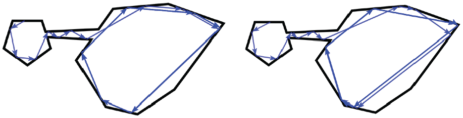
Two paths produced by different sequences of bounces, which visit different points of $\partial P$ , yet have the same sequence of edge collisions and high-level dynamical behavior (escape the room on the left, travel through hallway, then patrol the room on the right in a periodic orbit).

The present work is meant to serve as documentation of the data structures we have been developing to analyze bouncing robot systems, and a store for statements and proofs of mathematical properties thus far proven about the systems. The implications of our results for planning are broad, and depend on the desired application of the robotic system. In our case, we focus our examples on generating minimalist strategies such as constant bounce rules. We are interested both in the theoretical questions of what tasks are possible with such strategies, and in applications such as manufacture of micro-scale robots that use mechanical interactions with boundaries to execute the bounce rules and thus cannot be programmed with high-resolution strategies or complex on-board state estimation.

A preliminary version of a portion of this paper appeared in Nilles et al. (2018). The main differences are as follows.

We provide detailed proofs of all the theoretical statements presented in the preliminary version.

New theoretical results are included that characterize limit cycles in convex polygons and describe how they can be used to reduce uncertainty on the robot’s location.

Examples are presented that illustrate the actual execution of the navigation strategies provided by our planner.

The experimental evaluation of the proposed planner is further expanded through a reachability analysis, that is, an evaluation with respect to which parts of polygons are not reachable using the planner.

The main contributions of our work can be summarized by the following three ideas that simplify the characterization and generation of paths of the aforementioned mobile robots. The first idea is that we assume the robot has some intrinsic non-determinism. We would like our plans to have the property that they will succeed as long as the robot executes any action in an action set at each stage of execution. We can then analyze the size of the bounce rule sets at each stage to determine the minimum required accuracy of a successful robot design. In Section 3, we detail our assumptions on motion and formalize planning tasks. Our second contribution is that by using the geometric structure of a polygonal environment, we can create a combinatorial representation of the environment that lets us reason over a finite number of families of paths, instead of the infinite collection of all possible paths. Section 4 explains our discretization scheme and Section 5 provides some guarantees and limitations of planning with safe roadmaps using purely combinatorial and geometric information. Finally, in a third contribution, we provide results on when actions can be used to reduce non-determinism in the system. Geometrically, sometimes bounces can be made that will shrink the set of possible positions of the robot. In Section 6 we detail our steps toward leveraging this property in a planner.

Technical documentation of related softwares can be found online at: https://github.com/alexandroid000/bounce_viz

2. Related work

We incorporate techniques from computational geometry, specifically visibility (Ghosh, 2007). Visibility has been considered extensively in robotics, but usually with the goal of avoiding obstacles (Lozano-Pérez and Wesley, 1979; Siméon et al., 2000). To plan over collisions, we use the edge visibility graph, analyzed by O’Rourke and Streinu (1998), and shown to be strictly more powerful than the vertex visibility graph. Our work is also related to problems that consider what parts of a polygon will be illuminated by a light source after multiple reflections (as if the edges of the polygon are mirrors) (Aronov et al., 1998), or with diffuse reflections (Prasad et al., 1998), which are related to our non-deterministic bounces.

Our robot motion model is related to dynamical billiards (Tabachnikov, 2005). Modified billiard systems have attracted recent interest (Del Magno et al., 2014; Markarian et al., 2010; Tabachnikov, 2005). One similar work was inspired by the dynamics of microorganisms; Spagnolie et al. (2017) showed that Chlamydomonas reinhardtii“bounce” off boundaries at a specific angle determined by their body morphology. They characterize periodic and chaotic trajectories of such agents in regular polygons, planar curves, and other environments. Our model is especially interesting in this domain because high-fidelity state estimation and control is often not possible at small scales. It becomes necessary to make different assumptions about available motion primitives, and our assumptions are more physically realistic as micro-swimmers can often be constructed to have a default forward swimming behavior and have predictable, mechanical interactions with boundaries (Li and Ardekani, 2014).

Our motion model is a form of compliant motion, in which task constraints are used to guide task completion, even when the exact system state is not known. Our use of contraction mappings and non-deterministic reasoning is related to the idea of funnels: using the attraction regions of a dynamical system to guide states into a goal region. These ideas have been developed in the context of manipulation and fine motion control by Whitney (1977), Mason (1985), Erdmann (1986), Goldberg (1993), Lozano-Perez et al. (1984), Lynch and Mason (1995), and Burridge et al. (1999), among many others. What we term safe planning is also related to conformant planning (Anders et al., 2018), where given a set of possible initial configurations, a set of non-deterministic actions, and a set of goal configurations, the planner should find a sequence of actions guaranteed to bring the system into the goal.

Our intentional use of collisions with environment boundaries is enabled by the advent of more robust, lightweight mobile robots. Collisions as information sources have also been recently explored for multi-robot systems (Mayya et al., 2019). The first-class study of the dynamical properties of bouncing was proposed in Erickson and LaValle (2013) and continued in Nilles et al. (2017). Here we extend and improve these analysis tools, and incorporate visibility properties to discretize the strategy space. Work in contact planning for polygonal objects is very closely related, and we use similar techniques for discretizing and planning over the polygon boundary as seen in Allen et al. (2015); this caging problem is almost an “external” version of our problem, albeit without the aspect of long-term trajectory design.

Alam et al. (2017, 2018) described navigation, coverage, and localization algorithms for a robot that rotates a fixed amount relative to the robot’s prior heading. Owing to the chosen state space discretization, periodic trajectories may exist that require bounce angles not allowed by the discretization. By using a discretization induced by the environment geometry, we are able to find all possible limit cycles, and the controllers necessary to achieve them. Another closely related work is Lewis and O’Kane (2013), which considered navigation for a robot that has our same motion model, with uncertainty given as input to the algorithm. This uncertainty bound is used to create a boundary discretization using similar visibility properties as our approach, and the resulting discretized space is searched for plans. In our case, instead of taking error bounds as input, our approach considers all possible amounts of uncertainty, and returns bounds on the required accuracy for strategies. This group has also recently extended their approach to the coverage problem (Lewis et al., 2018).

We are working toward a generalization and hierarchy of robot models, in a similar spirit to Brunner et al. (2008). Their simple combinatorial robot is able to detect all visible vertices and any edges between them, and move straight toward vertices. By augmenting this basic robot model with sensors they construct a hierarchy of these robot models. Our questions are related but different: if the robot is given a compact, purely combinatorial environment representation, what tasks can it accomplish with minimal sensing, and how can we generate minimal complexity, robust plans?

3. Model and definitions

Next, we present the basic modeling of the addressed problem, describing the considered robotic system and the type of used environments. In addition, the concept of bounce rule is introduced, which is further used to formulate the concept of a bounce strategy.

We consider the movement of a point robot in a simple polygonal environment, potentially with polygonal obstacles. All index arithmetic for polygons with $n$ vertices is mod $n$ throughout this paper. We do not require polygons in general position. We do not consider trajectories that intersect polygon vertices. We define our robot to move forward in a straight line, until encountering an environment boundary (such as when a bump or range sensor is triggered). Once at a boundary, the robot is able to rotate in place. More formally, the model is as follows.

The configuration space $X = \partial P \times S^{1}$ , where $P$ is a simple polygon, potentially with holes. Here $P$ has boundary $\partial P$ , the union of external and obstacle boundaries, and $S^{1}$ is the robot’s orientation in the plane. Let $s$ refer to a point in $\partial P$ without an associated robot orientation.

The action space $U = [0, π]$ , where $u \in U$ is the orientation the robot takes when it reaches an environment boundary, before moving forward again. Here $u$ is measured counterclockwise relative to the boundary tangent.

The state transition function $f : X \times U \to X$ , which describes how actions change the state of the robot. We will often lift this function to act non-deterministically over sets of states and actions, propagating each state forward under each possible action, and uniting the resulting set of states.

We model time as proceeding in stages; at each stage $k$ , the robot is in contact with the environment boundary, executes an action $u_{k}$ , and then moves forward until the next contact with the boundary at stage $k + 1$ .

Definition 1. Let $α \in (0, π)$ be the robot’s incoming heading relative to the environment boundary at the point of contact. Let $θ \in (0, π)$ be a control parameter. A bounce rule $b$ maps $α$ and $θ$ to an action $u$ , and determines how the robot will reorient itself when it collides with a boundary. Bounce rules are defined in the frame in which the environment normal is aligned with the positive $y$ axis and the robot’s point of contact with the boundary is the origin.

Definition 2. A non-deterministic bounce rule is a bounce rule lifted to return a set of actions. We restrict non-deterministic bounce rules to return a convex set of actions (a single interval in $(0, π)$ ).

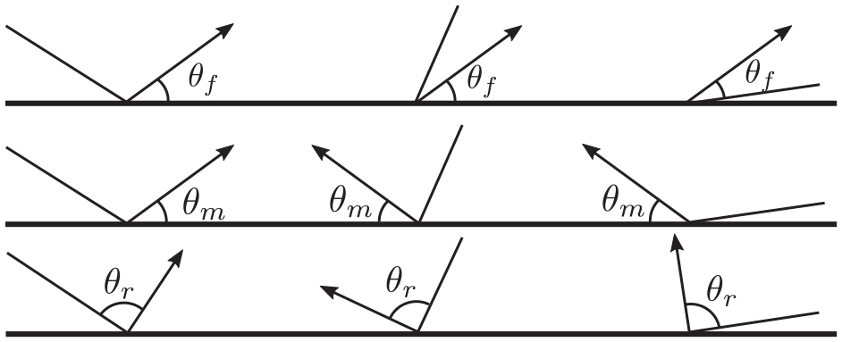
For example, a specular bounce (laser beams, billiard balls) has bounce rule $b (α, θ) = π - α$ . See Figure 2 for more examples of bounce rules.

Fig. 2.

Examples of different “bounce rules” that can be implemented on mobile robots. In the first row, $b (α, θ) = θ_{f}$ , which we refer to as a fixed bounce rule. In the second row, we have a monotonic fixed bounce rule, in which $b (α, θ) = θ_{m}$ or $π - θ_{m}$ , depending on what is necessary to preserve monotonicity of travel direction along the $x$ axis. In the third row, we have a relative bounce rule, $b (α, θ) = α - θ_{r}$ , rotating $α$ through $θ_{r}$ in the clockwise direction. If this rotation causes the heading of the robot to still be facing into the boundary, the robot performs the rotation again until its heading points into the free space.

Definition 3. A bounce strategy is a sequence of non-deterministic bounce rules.

Of course, robots rarely move perfectly, so our analysis will assume the robot has some non-determinism in its motion execution. Instead of modeling explicit distributions, we assume the robot may execute any action in a set. Planning over such non-determinism can result in design constraints for robots; for example, if a robot has an uncertainty distribution over its actions in the range $u \pm ϵ$ , the largest allowable $ϵ$ will be half the width of the smallest convex bounce rule interval in a strategy.

4. Visibility-based boundary partitioning

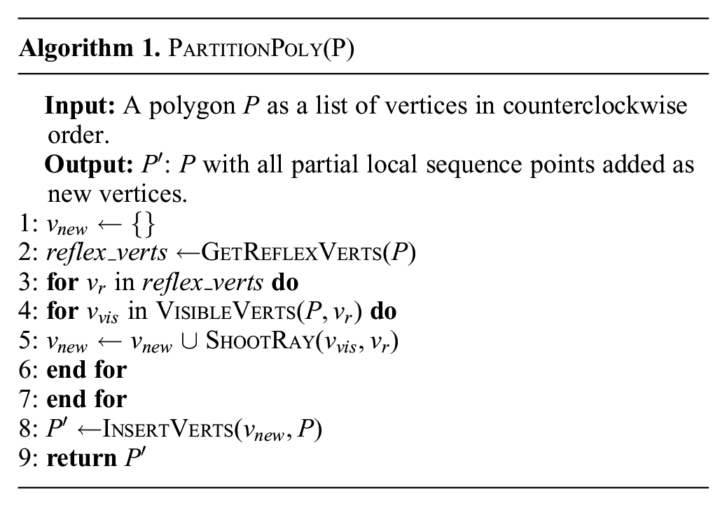
In this section, the bounce visibility graph is introduced. Such a graph is a combinatorial structure that is queried to obtain plans in the form of sequences of bouncing rules, namely, queried to obtain bounce strategies. To introduce the bounce visibility graph, we start by recalling the definition of the visibility polygon, which is used to define a partial local sequence of points on the environment boundary at which the visibility polygon changes structure. The partial local sequence, whose computation is summarized in Algorithm 1, is then used to define the edge visibility graph. The bounce visibility graph is defined as the directed version of the edge visibility graph. We now proceed to provide the specifics.

Algorithm 1. PartitionPoly(P)
Input: A polygon $P$ as a list of vertices in counterclockwise order.
Output: $P'$ : $P$ with all partial local sequence points added as new vertices.
1: $v_{new} \leftarrow {}$
2: $reflex_verts \leftarrow$ GetReflexVerts( $P$ )
3: for $v_{r}$ in $reflex_verts$ do
4: for $v_{vis}$ in VisibleVerts( $P, v_{r}$ ) do
5: $v_{new} \leftarrow$ $v_{new} \cup$ ShootRay( $v_{vis}, v_{r}$ )
6: end for
7: end for
8: $P' \leftarrow$ InsertVerts( $v_{new}, P$ )
9: return $P'$

Algorithm 2. SafeConstantFixedNavigate( $P$ , $S$ , $G$ , $k$ )
Input: A polygon $P$ , intervals $S$ and $G$ in $\partial P$ , and an integer bound $k$ .
Output: A non-deterministic bounce rule, or None if no strategy can be found. [1]
1: $P' \leftarrow$ PartitionPoly( $P$ )
2: $BVG \leftarrow$ mkBVG( $P'$ )
3: $BV G_{safe} \leftarrow$ mkSafeBVG( $BVG$ )
4: $\tilde{θ} \leftarrow$ SearchConstantFixedStrats( $BV G_{safe}$ , $S$ , $G$ , $k$ )
5: return $\tilde{θ}$

Given a polygonal environment (such as the floor plan of a warehouse or office space), we would like to synthesize bounce strategies that allow a robot to perform a given task (such as navigation or patrolling). To do so, we first discretize the continuous space of all possible transitions between points on $\partial P$ . We find a visibility-based partition that encodes the idea of some points on $\partial P$ having different available transitions.

Definition 4. The visibility polygon of a point $s$ in a polygon $P$ is the polygon formed by all the points in $P$ that can be connected to $s$ with a line segment that lies entirely within $P$ .

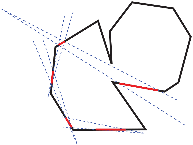
Imagine a robot sliding along the boundary of a polygon, calculating the visibility polygon as it moves. In a convex polygon, nothing exciting happens. In a non-convex polygon, the reflex vertices (vertices with an internal angle greater than $π$ ) cause interesting behavior. As the robot slides, its visibility polygon mostly changes continuously. Edges shrink or grow, but the combinatorial structure of the polygon remains the same, until it aligns with a reflex vertex $r$ and another vertex $v$ (visible from $r$ ). At this point, either $v$ will become visible to the robot, adding an edge to the visibility polygon, or $v$ will disappear behind $r$ , removing an edge from the visibility polygon.

To compute all such points at which the visibility polygon changes structure, we compute the partial local sequence, defined in O’Rourke and Streinu (1998). These are, equivalently, the points where the combinatorial visibility vector changes, as defined in Suri et al. (2008). Each point in the partial local sequence marks the point at which a visible vertex appears or disappears behind a reflex vertex. 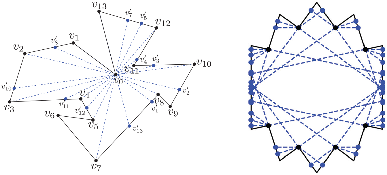The sequence is constructed by shooting a ray through each reflex vertex $r$ from every visible vertex and keeping the resulting sequence of intersections with $\partial P$ . See Figure 3 for an example of the vertices in the partial local sequence of $v_{0}$ .

Fig. 3.

On the left, the partial local sequence for $v_{0}$ . On the right, an example polygon for which the bounce visibility graph has $O (n^{4})$ edges.

Once all the partial local sequences have been inserted into the original polygon, the resulting segments have the property that any two points in the segment can see the same edge set of the original polygon (though they may see different portions of those edges). See Algorithm 1 for a pseudocode description of this partitioning process. Algorithm 1 applies to polygons with or without holes; holes require more bookkeeping to correctly find visible vertices and shoot rays. See Figure 4 for an example partition of a polygon with holes. 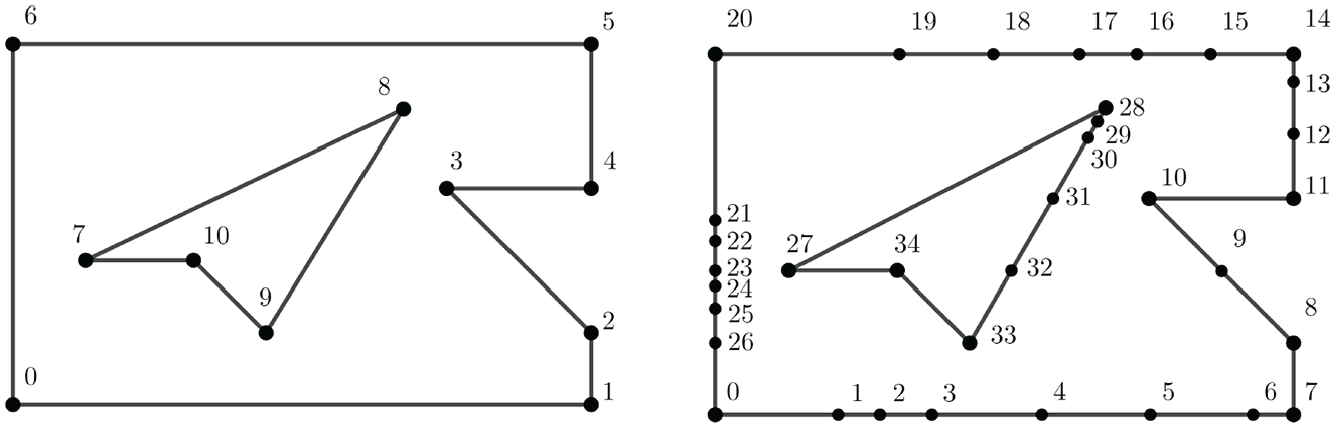Let $P'$ be the polygon $P$ after application of Algorithm 1.

Fig. 4.

An example partition for a polygon with holes; our discretization scheme extends naturally to handle visibility events caused by static obstacles.

The ShootRay function takes two visible vertices $v_{1}$ and $v_{2}$ and compute the first intersection of $\partial P$ and ray $v_{1} v_{2}$ . This operation will take $O (\log n)$ time after preprocessing the polygon $P$ in $O (n)$ (Szirmay-Kalos and Márton, 1998). The VisibleVerts function computes all visible vertices in the polygon given an input query vertex, and takes $O (n)$ (El Gindy and Avis, 1981). Thus, the total runtime of Algorithm 1 is $O (n^{2} \log n)$ .

Definition 5. The edge visibility graph of a polygon $P$ has a node for each edge of $P$ , and has an arc between two nodes $(e_{i}, e_{j})$ if and only if there is a point $s_{i}$ in the open edge $e_{i}$ and a point $s_{j}$ on the open edge $e_{j}$ such that $s_{i}$ and $s_{j}$ can be connected with a line segment which is entirely within the interior of $P$ .

Let the bounce visibility graph be the directed edge visibility graph of $P'$ . Although visibility is a symmetric property, we use directed edges in the bounce visibility graph so that we can model the geometric constraints on the visibility from one edge to another, which are not symmetric and govern what actions allow the robot to accomplish that transition. See Section 5 for further exploration of this idea.

Proposition 1. The bounce visibility graph for a polygon with $n$ vertices has $O (n^{2})$ vertices and $O (n^{4})$ edges.

Proof. Consider a polygon $P$ with $n$ vertices operated on by Algorithm 1 to form $P'$ . Each convex vertex will not add any new vertices; however, a reflex vertex can add $O (n)$ new vertices. Up to half of the vertices in the polygon can be reflex, so the number of vertices in $P'$ is $O (n^{2})$ . Each vertex indexes a node in the edge visibility graph of $P'$ . A vertex in $P'$ may be visible to all other vertices, so in the worst case, the bounce visibility graph will have $O (n^{4})$ edges.□

4.0.1. Worst-case example for Algorithm 1

We might hope that if $r$ is large, then not all of the reflex vertices will produce a large number of new vertices, and we may bound the size of the edge set in the visibility graph. Unfortunately, the number of reflex vertices, the new vertices produced in their partial local sequence, and the new vertices’ visibility can be large at the same time. We present a family of input polygons with bounce visibility graph edge-set size of $O (n^{4})$ .

Let $n = 4 t + 2$ , in which $t$ is a positive integer. We design a polygon with $r = 2 t$ reflex vertices. The polygon is symmetric with respect to its medium horizontal line. In the top half, the reflex vertices are uniformly located on a circle and thus they are visible to each other; the convex vertices are chosen so that they are outside the circle and the line through an edge will not intersect other edges. Each reflex vertex will have at least $t - 1$ new vertices in its partial local sequence. There will be $2 t (t - 1) + n$ vertices in the polygon after we insert all new vertices in the partial local sequence for all reflex vertices. Each of them can see at least $t (t - 1) + n / 2$ other vertices. Thus, the number of edges in the transition graph for the polygon with inserted vertices is $O ((2 t (t - 1) + n) (t (t - 1) + n / 2)) = O (t^{4}) = O (n^{4})$ . Figure 3 shows the polygon for $t = 4$ with all the vertices in the partial local sequences.

5. Safe actions

To characterize some families of paths, we use the boundary partition technique defined in Section 4, then define safe actions between segments in the partition that are guaranteed to transition to the same edge from anywhere in the originating edge. Such actions define transitions which keep the robot state in one partition under non-deterministic actions.

Definition 6 establishes a notion of visibility between two edges in a polygon. Later, Definition 7 formally introduces the safe actions. Through Definitions 6 and 7, Proposition 2 provides bounce angle intervals that describe safe actions. Lemma 1 and Corollary 1 exhibit scenarios for which safe actions exists between two edges of a polygon. Finally, Proposition 3 establishes a result on the existence of at least two safe actions for every edge in a polygon that was partitioned utilizing Algorithm 1 (see Section 4). The proof of Proposition 3 makes use of some auxiliary definitions presented in Definition 8.

Definition 6. Two edges $e_{i}, e_{j}$ of a polygon are entirely visible to each other if and only if every pair of points $s_{i} \in e_{i}$ and $s_{j} \in e_{j}$ are visible (the shortest path between $s_{i}$ and $s_{j}$ lies entirely within $P$ ).

Definition 7. A safe action from edge $e_{i}$ to edge $e_{j}$ in a polygon is an action $u$ such that $f (s, u) \in e_{j}$ for any $s \in e_{i}$ and $u$ in some interval of actions $\tilde{θ} \subseteq (0, π)$ .

Proposition 2. Given two entirely visible line segments $e_{i} = (v_{i}, v_{i + 1})$ and $e_{j} = (v_{j}, v_{j + 1})$ in $\partial P'$ , if a safe action exists from $e_{i}$ to $e_{j}$ , the maximum interval of safe actions is $\tilde{θ} = [θ_{r}, θ_{l}]$ such that $θ_{r} = π - ∠ v_{j} v_{i + 1} v_{i}$ and $θ_{l} = ∠ v_{j + 1} v_{i} v_{i + 1}$ .

Proof. Let edge $e_{i} = (v_{i}, v_{i + 1})$ be aligned with the positive $x$ axis with the clockwise endpoint at the origin, without loss of generality. Owing to the edges being entirely visible, $e_{j} = (v_{j}, v_{j + 1})$ must be in the top half of the plane, above $e_{i}$ .

Take the quadrilateral formed by the convex hull of the edge endpoints. Let the edges between $e_{i}$ and $e_{j}$ be $e_{l} = (v_{i}, v_{j + 1})$ and the right-hand edge $e_{r} = (v_{i + 1}, v_{j})$ . Let $θ_{l}$ be the angle between $e_{l}$ and the positive $x$ axis ( $0 < θ_{l} < π$ ); similarly for $e_{r}$ and $θ_{r}$ . See Figure 5 for an illustration of the setup.

Fig. 5.

Angle range such that a transition exists for all points on originating edge (left: such a range exists; right: such a range does not exist).

There are three cases to consider: if $e_{l}$ and $e_{r}$ are extended to infinity, they cross either above or below edge $e_{i}$ , or they are parallel.

Case 1: $e_{l}$ and $e_{r}$ meet below edge $e_{i}$ . In this case, $θ_{l} > θ_{r}$ and if a ray is cast from any point on $e_{i}$ at angle $θ \in [θ_{r}, θ_{l}]$ , the ray is guaranteed to intersect $e_{j}$ in its interior.

Case 2: $e_{l}$ and $e_{r}$ meet above edge $e_{i}$ . In this case, $θ_{l} < θ_{r}$ , and there is no angle $θ$ such that a ray shot from any point on $e_{i}$ will intersect $e_{j}$ . To see this, imagine sliding a ray at angle $θ_{l}$ across the quadrilateral: at some point before reaching $v_{i + 1}$ , the ray must stop intersecting $e_{j}$ , otherwise we would have $θ_{l} > θ_{r}$ .

Case 3: $e_{l}$ and $e_{r}$ are parallel. This implies that $θ_{l} = θ_{r}$ , which is the only angle for which a transition from any point on $e_{i}$ is guaranteed to intersect $e_{j}$ , and $\tilde{θ}$ is a singleton set.

Thus, for each case, we can either compute the maximum angle range or determine that no such angle range exists. □

Note that this definition of a safe action is similar to the definition of an interval of safe actions from Lewis and O’Kane (2013); the main differences in approach are the generation of boundary segments, methods of searching the resulting graph, and how we generate constraints on robot uncertainty instead of assuming uncertainty bounds are an input to the algorithm.

Lemma 1. If two edges in $\partial P'$ are entirely visible to each other, then there will be at least one safe action between them.

Proof. From the proof of Proposition 2, we can see that if case one holds in one direction, case two will hold in the other direction, so a safe action must exist from one edge to the other in one direction. If case three holds, there is a safe action both directions but $\tilde{θ}$ is a singleton set.□

Corollary 1. If two edges in $\partial P'$ share a vertex that is not reflex, and the two edges are not collinear, then there exist safe actions from one to the other in both directions.

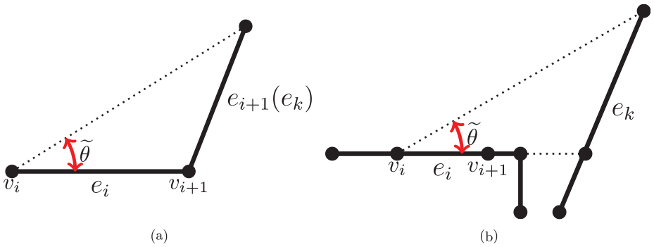
For a proof of Corollary 1, see Figure 6(a). Algorithm 1 guarantees that such neighboring segments are entirely visible.

Fig. 6.

Examples of a geometrical setup for some guaranteed safe actions.

Definition 8. Given two entirely visible segments $e_{i}$ and $e_{j}$ , rotate the frame such that $e_{i}$ is aligned with the $x$ axis with its normal pointing along the positive $y$ axis, such that segment $e_{j}$ is above segment $e_{i}$ . If the intersection of segment $e_{i}$ and $e_{j}$ would be on the left of segment $e_{i}$ , then call the transition from $e_{i}$ to $e_{j}$ a left transition; if the intersection would be on the right of segment $e_{i}$ , then call the transition a right transition.

Proposition 3. For every polygon $P$ and the resulting partitioned polygon $P'$ under Algorithm 1 , each edge $e \in P'$ has at least two safe actions that allow transitions away from $e$ .

Proof. Let $e_{i} = (v_{i}, v_{i + 1})$ . Consider right transitions from $e_{i}$ to some $e_{k}$ , where the safe action interval $\tilde{θ} = (0, θ_{l})$ for some non-zero $θ_{l}$ . We show that such a transition must exist.

By Corollary 1, if an edge $e_{i}$ has an adjacent edge $e_{i + 1}$ that is not collinear or separated by a reflex angle, $e_{k} = e_{i + 1}$ and a safe transition exists between $e_{i}$ and $e_{i + 1}$ with $θ_{l} = ∠ v_{i + 2} v_{i} v_{i + 1}$ . See Figure 6(a).

If the adjacent edge is at a reflex angle, Algorithm 1 will insert a vertex in line with $e_{i}$ on the closest visible edge, forming edge $e_{k}$ . If $v_{i}$ is an original vertex of $P$ , $e_{k}$ will be entirely visible from $e_{i}$ , because Algorithm 1 will otherwise insert a point in the partial local sequence of $v_{i}$ .

If $v_{i}$ is itself inserted by Algorithm 1, $e_{k}$ will still be entirely visible. There must be some original vertex of $P$ clockwise from $v_{i}$ and collinear with $e_{i}$ , which would insert a vertex visible to $e_{i}$ through Algorithm 1 if there were any reflex vertices blocking transitions to $e_{k}$ . See Figure 6(b) for an example of the geometry.

If the adjacent edge $e_{i + 1}$ is collinear with $e_{i}$ , apply the previous reasoning to the first non-collinear edge to find $e_{k}$ . The arguments extend symmetrically to left transitions, which will have safe actions of the form $\tilde{θ} = [θ_{r}, π)$ . Thus, each edge will have two guaranteed safe actions leading away from it.□

6. Dynamical properties of paths

Many robot tasks can be specified in terms of dynamical properties of the path the robot takes through space, such as stability, ergodicity, and reachability. Our motion strategy allows us to disregard the robot’s motion in the interior of $P$ . Instead, the robot’s state is an interval along the boundary $\partial P$ , and we can formulate transitions as a discrete dynamical system under the transition function $f$ . The properties of this dynamical system can be used to engineer paths corresponding to different robot task requirements.

One generally useful property of mapping functions is contraction: when two points under the function always become closer together. We can use this property to control uncertainty in the robot’s position.

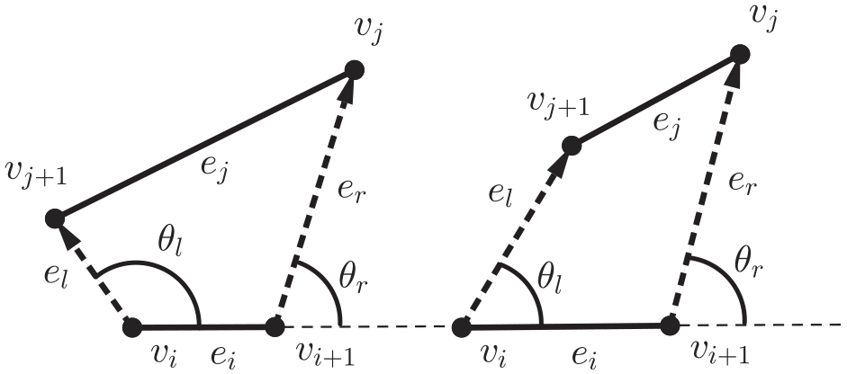
We now proceed as follows. Definition 9 presents some notation useful for the remainder of this section. Definition 10 recalls the general concept of a contraction mapping that is useful to model the dynamical properties of paths to be followed by the robot. Based on the already introduced notation, Lemma 2 establishes bounce angles for which function $f$ , a transition function that models bounces between edges in $P$ , is a contraction mapping. Corollary 2 extends the results of Lemma 2 for specific types of pairs of edges. Alternatively, a mapping can be identified as a contraction mapping by analyzing what is known as the contraction coefficient. Definition 11 formally introduces such concept of a contraction coefficient, and Definition 12 expands that concept for the case of a composition of transitions between a sequence of edges. Such composition, when it comes to a contraction mapping, is used in following subsections to model limit cycles, namely, paths that eventually return the robot to its start position.

Definition 9. Let $ϕ_{i, j}$ be the interior angle between two edges $e_{i}, e_{j} \in \partial P$ .

Definition 10. A function $g$ that maps a metric space $M$ to itself is a contraction mapping if for all $x, y \in M$ , $| g (x) - g (y) | \leq c | x - y |$ , and $0 \leq c < 1$ .

Lemma 2. If the transition from segment $e_{i}$ to segment $e_{j}$ is a left transition, then the transition function $f (x, θ)$ between segments $e_{i}$ and $e_{j}$ is a contraction mapping if and only if $θ > \frac{π}{2} + \frac{ϕ_{i, j}}{2}$ ; if a right transition, the transition function $f (x, θ)$ is a contraction mapping if and only if $θ < \frac{π}{2} - \frac{ϕ_{i, j}}{2}$ .

Proof. We consider the two cases of transition separately.

For the transition shown in the left-hand side of Figure 7,

$\bar{xf (x, θ)} ∥ \bar{yf (y, θ)} \Rightarrow \frac{| f (x, θ) - f (y, θ) |}{| x - y |} = \frac{| f (x, θ) |}{| x |} = \frac{\sin (π - θ)}{\sin (θ - ϕ_{i, j})} = \frac{\sin (θ)}{\sin (θ - ϕ_{i, j})}$

The transition will be contraction if and only if $\frac{| f (x, θ) - f (y, θ) |}{| x - y |} < 1 \Leftrightarrow \sin (θ) < \sin (θ - ϕ_{i, j})$ . If $θ < \frac{π}{2}$ , then $\sin (θ) > \sin (θ - ϕ_{i, j})$ . Thus, we need $θ > \frac{π}{2}$ . If $θ - ϕ_{i, j} > \frac{π}{2}$ , then $\sin (θ) < \sin (θ - ϕ_{i, j})$ and we are done; otherwise, we need $π - θ < θ - ϕ_{i, j} \Rightarrow θ - \frac{ϕ_{i, j}}{2} > \frac{π}{2}$ . Combining all conditions, we have the transition will be contraction if and only if $θ > \frac{π}{2} + \frac{ϕ_{i, j}}{2}$ .

Similarly, for a right transition shown in the right-hand side diagram of Figure 7,

$\bar{xf (x, θ)} ∥ \bar{yf (y, θ) \Rightarrow \frac{| f (x, θ) - f (y, θ) |}{| x - y |} = \frac{| f (x, θ) |}{| x |} = \frac{\sin (π - θ)}{\sin (π - θ - ϕ_{i, j})} = \frac{\sin (θ)}{\sin (θ + ϕ_{i, j})}}$

The transition will be contraction if and only if $\frac{| f (x, θ) - f (y, θ) |}{| x - y |} < 1 \Leftrightarrow \sin (θ) < \sin (θ + ϕ_{i, j})$ . If $θ > \frac{π}{2}$ , then $\sin (θ) > \sin (θ + ϕ_{i, j})$ . Thus we need $θ < \frac{π}{2}$ . If $θ + ϕ_{i, j} < \frac{π}{2}$ , then $\sin (θ) < \sin (θ + ϕ_{i, j})$ and we are done; otherwise, we need $θ < π - θ - ϕ_{i, j} \Rightarrow θ < \frac{π}{2} - \frac{ϕ_{i, j}}{2}$ . Combining all conditions, we have the transition will be contraction if and only if $θ < \frac{π}{2} - \frac{ϕ_{i, j}}{2}$ .□

Fig. 7.

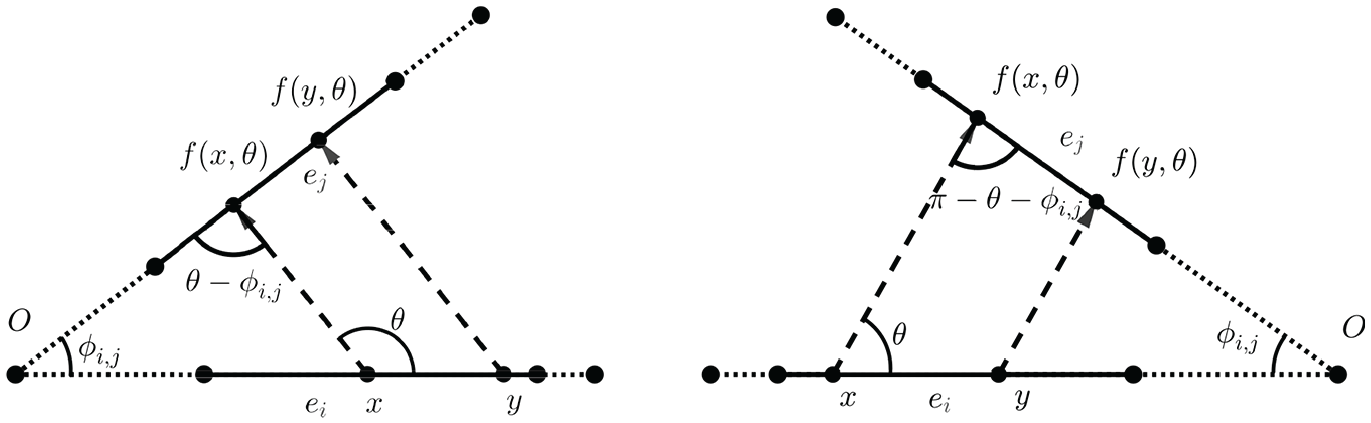
The two cases for computing contraction mapping conditions.

Corollary 2. For all pairs of adjacent segments with internal angle less than $π$ , there exists a range of actions for which $f$ is a contraction mapping.

Definition 11. The contraction coefficient of a mapping is the ratio of the distance between points before and after the mapping is applied. Let $C (θ, ϕ_{i, j})$ be the contraction coefficient of a transition from $e_{i}$ to $e_{j}$ in $\partial P$ For a left transition, $C (θ, ϕ_{i, j}) = | \frac{\sin (θ)}{\sin (θ - ϕ_{i, j})} |$ ; for a right transition, $C (θ, ϕ_{i, j}) = | \frac{\sin (θ)}{\sin (θ + ϕ_{i, j})} |$ .

Given $C$ from Definition 11, for a sequence of transitions $f_{0}, \dots, f_{k}$ , we can construct the overall mapping from the domain of $f_{0}$ to the range of $f_{k}$ through function composition. As $f$ is a linear mapping, the contraction coefficient of a composition of multiple bounces can be determined by multiplying the contraction coefficients of each bounce.

Definition 12. Given a sequence of $m$ feasible transitions $F = {f_{0}, f_{1}, \dots, f_{m - 1}}$ , at stage $k$ the robot will be located on edge $e (k)$ and will depart the edge with action $θ_{k}$ ; the contraction coefficient of the overall robot trajectory $f_{m - 1} ° \dots ° f_{0}$ is $C (F) = Π_{k = 0}^{m - 1} C (θ_{k}, ϕ_{e (k), e (k + 1)})$ .

If $C (F) < 1$ , the composition of $F$ is a contraction mapping. This is true even if some transition along the way is not a contraction mapping, because $C (F)$ is simply the ratio of distances between points before and after the mapping is applied. Furthermore, the value of $C (F)$ tells us the exact ratio by which the size of the set of possible robot states has changed.

6.1. Limit cycles

A contraction mapping that takes an interval back to itself has a unique fixed point, by the Banach fixed point theorem (Granas and Dugundji, 2003). By composing individual transition functions between edges, we can create a self-mapping by finding transitions which take the robot back to its originating edge. A fixed point of this mapping corresponds to a stable limit cycle. The usefulness of the limit cycles is that it is possible to find bounce strategies that make the robot’s trajectory converge to a limit cycle. Those bounce strategies can be used to delimit the possible positions the robot might be in, for example, to localize the robot, or even to make the robot move repetitively along a trajectory, as it is desirable in a patrolling task. Such trajectories in regular polygons were characterized in Nilles et al. (2017). Here, we present a more general proof for the existence of limit cycles in all convex polygons.

More precisely, Theorem 1 characterizes the limit cycles in convex polygons, that is, it provides the exact location of such a cycle in terms of its contact points in $\partial P$ . For achieving that goal, Definition 13 introduces some notation, followed by Lemma 3 that describes sufficient conditions on the bounce angles for a limit cycle to exist in any convex polygon. We conclude the subsection with Proposition 4, which establishes the existence of a particular bounce strategy that makes the robot to enter a limit cycle.

Definition 13. The smallest interior angle in a polygon $P$ is $ϕ_{P, \min}$ .

Lemma 3. Consider $θ \in (0, \frac{π}{2}]$ , if

\begin{matrix} θ \in (0, min (min_{i = 0, 1, \dots, n - 1} (∠ v_{i + 2} v_{i} v_{i + 1}), min_{i = 0, 1, \dots, n - 1} \\ (\frac{π}{2} - \frac{ϕ_{i - 1, i}}{2}))), \end{matrix}

then the fixed bounce rule $b (α, θ) = θ$ leads to a convex cycle that visits each edge of $P$ sequentially, regardless of the robot’s position. For all convex polygons with $n$ edges, there exist constant fixed-angle bouncing strategies which result in a period $n$ limit cycle regardless of the robot’s start position.

Proof. See Figure 8 for the geometric setup.

Fig. 8.

The notation setup for the proof of contracting cycle in a convex polygon.

Without loss of generality, assume $θ \in (0, \frac{π}{2}]$ . The robot will always bounce to the next adjacent edge if and only if $θ \in (0, min_{i} (∠ v_{i + 2} v_{i} v_{i + 1}))$ .

Suppose we have two start positions $s_{1}$ and $s_{2}$ on edge $e_{0}$ and a constant fixed bounce rule $b (α, θ) = θ$ . At stage $k$ , $s_{1}$ and $s_{2}$ will be located at $f^{k} (s_{1}, θ)$ and $f^{k} (s_{2}, θ)$ .

By Definition 12, the distance between $s_{1}$ and $s_{2}$ changes after one orbit of the polygon by the ratio $\frac{| f^{n} (s_{1}, θ) - f^{n} (s_{2}, θ) |}{| s_{1} - s_{2} |} = Π_{i = 0}^{n - 1} C (θ, ϕ_{i, i + 1})$ . If this ratio is less than one, then $f^{n} (s, θ)$ has a unique fixed point by the Banach fixed-point theorem (Granas and Dugundji, 2003). By Lemma 2, this constraint is satisfied if $θ < \frac{π}{2} - \frac{ϕ_{i, i + 1}}{2}$ for all $i$ . We can guarantee that this condition holds for the orbit by requiring

\begin{matrix} θ \in (0, min (min_{i = 0, 1, \dots, n - 1} (∠ v_{i + 2} v_{i} v_{i + 1}), \\ min_{i = 0, 1, \dots, n - 1} (\frac{π}{2} - \frac{ϕ_{i - 1, i}}{2}))), \end{matrix}

in which case the fixed-angle bouncing strategy with $b (α, θ) = θ$ leads to a convex cycle that visits each edge of $P$ sequentially, regardless of the robot’s start position. Symmetry applies for orbits in the opposite direction.□

Thus, now we know that such cycles must exist in convex polygons, and we know the conditions on fixed bounce laws that will create them, but we can also compute exactly where these cycles would be located (in the asymptotic limit).

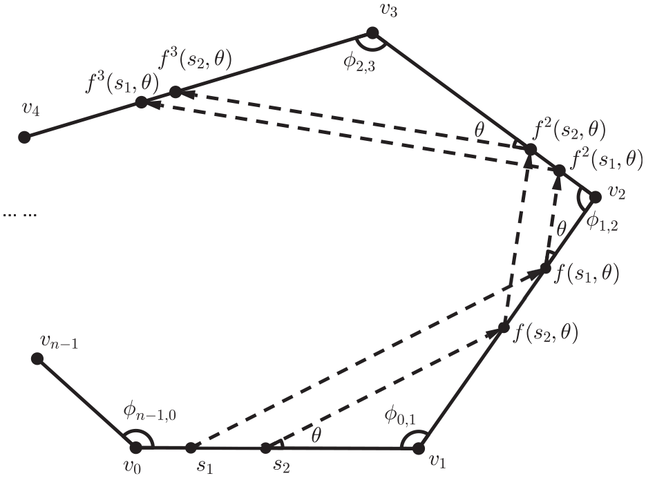
For ease of notation, Theorem 1 will compute the location of counterclockwise limit cycle trajectories as a fixed point of the return map of the trajectory starting on edge $e_{0}$ . The rest of the points of the limit cycle can be computed from forward projection of the trajectory, or from reindexing the vertices and computing this distance for each edge. Clockwise limit cycles can be computed through symmetry (flipping the polygon in the plane and computing the cycle, then flipping back).

Theorem 1. Under a fixed bounce rule $b (α, θ) = θ$ in a convex polygon with $n$ edges, if $θ$ satisfies the conditions in Lemma 3 such that the trajectory will converge asymptotically to a limit cycle striking each sequential edge of the polygon in counter-clockwise order, then on edge $e_{0}$ the limit cycle will be located distance

d_{FP} = \frac{\sum_{j = 0}^{n - 1} {(- 1)}^{n - j - 1} ℓ_{j} Π_{k = j}^{n - 1} C (θ, ϕ_{k, k + 1})}{1 - {(- 1)}^{n} Π_{k = 0}^{n - 1} C (θ, ϕ_{k, k + 1})},

(1)

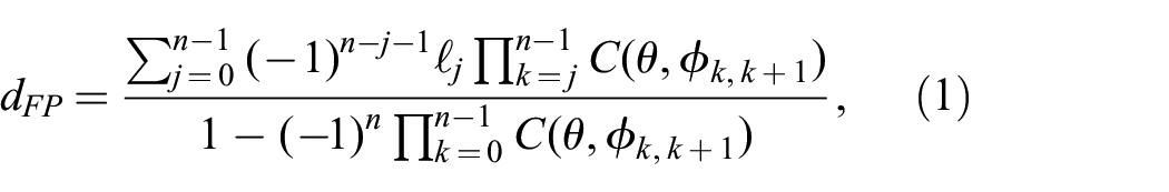
from vertex $v_{0}$ .

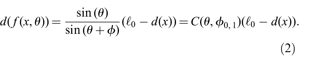
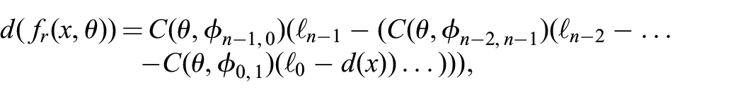
Proof. Define a distance function, $d$ , which measures the robot’s linear distance along the polygon boundary from the nearest clockwise vertex. If the robot bounces at angle $θ$ between edges $e_{i}$ and $e_{i + 1}$ , the new distance $d (f (x, θ))$ can be derived with the law of sines as

d (f (x, θ)) = \frac{\sin (θ)}{\sin (θ + ϕ)} (ℓ_{0} - d (x)) = C (θ, ϕ_{0, 1}) (ℓ_{0} - d (x)) .

(2)

Now we define the return map, $f_{r}$ , corresponding to bouncing $n$ times around an $n$ -sided polygon until the robot returns to the originating edge. The new distance of the returning robot from $v_{0}$ can be computed by composing the distance functions of each transition, of the form in Equation (2). This return map will take the form

\begin{matrix} d (f_{r} (x, θ)) = C (θ, ϕ_{n - 1, 0}) (ℓ_{n - 1} - (C (θ, ϕ_{n - 2, n - 1}) (ℓ_{n - 2} - \dots \\ - C (θ, ϕ_{0, 1}) (ℓ_{0} - d (x)) \dots))), \end{matrix}

which can be expanded and grouped into

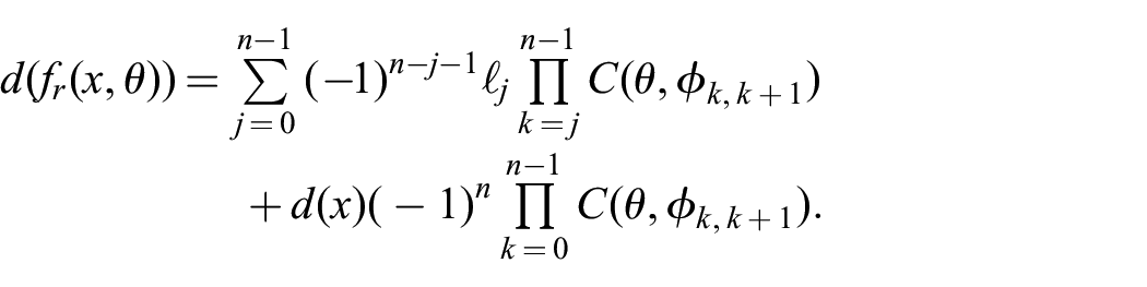
\begin{matrix} d (f_{r} (x, θ)) = \sum_{j = 0}^{n - 1} {(- 1)}^{n - j - 1} ℓ_{j} Π_{k = j}^{n - 1} C (θ, ϕ_{k, k + 1}) \\ + d (x) (- {1)}^{n} Π_{k = 0}^{n - 1} C (θ, ϕ_{k, k + 1}) . \end{matrix}

To find the fixed point of this return map (corresponding to the stable limit cycle of the robot around the polygon), we set $d (f_{r} (x, θ)) = d (x)$ , and solve for $d (x)$ , yielding

d (x) = \frac{\sum_{j = 0}^{n - 1} {(- 1)}^{n - j - 1} ℓ_{j} Π_{k = j}^{n - 1} C (θ, ϕ_{k, k + 1})}{1 - {(- 1)}^{n} Π_{k = 0}^{n - 1} C (θ, ϕ_{k, k + 1})},

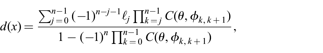
which, in turn, yields the expression for the distance $d_{FP}$ from vertex $v_{0}$ that defines the fixed point. □

Although Equation (1) might look cumbersome, it is easy to compute (linear in the number of sides of the polygon). See Figure 9 for an example of the predicted locations of the limit cycle in a convex polygon. The trajectory begins on the left hand side of the polygon and quickly converges to the predicted limit cycle.

Fig. 9.

Example of the predicted locations of the limit cycle in a convex polygon. The blue arrows indicate an example trajectory for a constant fixed bounce rule. Yellow circles indicate the predicted collision points of the asymptotically stable limit cycle for this bounce rule and polygon.

Proposition 4. For all points $s$ on the boundary of all polygons, a constant fixed-angle controller exists that will cause the robot’s trajectory to enter a stable limit cycle.

Proof. First we observe that by Proposition 3, for every segment $e \in \partial P'$ , safe actions always exist for two action intervals. These intervals are the ones bordering the segment itself: by staying close enough to the boundary, the robot may guarantee a safe transition. By Lemma 2, these safe actions will also admit contraction mappings. Thus, we may choose a constant fixed-angle controller such that it results in safe, contracting transitions from all segments in $P'$ . As there are a finite number of segments in $P'$ , this controller must result in limit cycle from every point in $P$ . If $s$ is on a hole of the polygon, this procedure will cause the robot to leave the hole and enter a cycle on the exterior boundary.□

6.2. Leveraging cycles to reduce uncertainty

Next, we detail how such cycles can be used to decrease uncertainty in the robot’s position. More precisely, if the robot utilizes a controller as that depicted in Proposition 4, then its path converges to a limit cycle and, as a consequence, the uncertainty on the knowledge of the robot’s whereabouts decreases.

Recalling that the fixed point of a cycle’s transition function represents the location of the respective limit cycle in $\partial P$ , then Corollary 3 provides a bound on the distance between the robot’s position and the cycle’s fixed point as the robot iterates $F$ , that is, as the robot keeps moving according to $F$ . Finally, Corollary 4 provides the number of cycles that the robot needs to traverse to find itself within a distance $ε$ from the fixed point.

Corollary 3. Choose a sequence of transitions $F$ that begins and ends on edge $e_{i}$ . Let the contraction coefficient of this trajectory be $C$ , and let the length of edge $e_{i}$ be $ℓ_{i}$ . After $k$ iterations of the cycle, the distance between the robot’s position and the fixed point of the cycle’s transition function must be less than $C^{k} ℓ_{i}$ .

Proof. The initial distance between the robot’s position and the fixed point of the cycle, $| x_{0} - x_{FP} |$ , is upper bounded by $ℓ_{i}$ . After $F$ has been executed once, the contraction ratio $C = \frac{| F (x_{0}) - F (x_{FP}) |}{| x_{0} - x_{FP} |} = \frac{| F (x_{0}) - x_{FP} |}{| x_{0} - x_{FP} |}$ , which implies $| F (x_{0}) - x_{FP} | = C | x_{0} - x_{FP} | \leq C ℓ_{i}$ . When $F$ is iterated $k$ times, this expression becomes $| F^{k} (x_{0}) - x_{FP} | \leq C^{k} ℓ_{i}$ .□

Corollary 4. If we assume the robot’s initial location lies in an interval on edge $e_{i}$ , and the robot performs a sequence of transitions $F$ that creates a cycle returning to $e_{i}$ with contraction coefficient $C$ , the size of the set of possible locations of the robot on edge $e_{i}$ will become less than $ϵ$ after $⌈ \log (ϵ / 2 ℓ_{i}) / \log (C) ⌉$ iterations of the cycle.

Proof. From Corollary 3, after $k$ cycles the distance between the robot’s position and the fixed point will be less than $C^{k} ℓ_{i}$ . Thus, if we wish for the size of the interval of possible positions to be less than $ϵ$ , we must have that $C^{k} ℓ_{i} = ϵ / 2$ . Solving for $k$ yields the expression above.□

7. Applications

7.1. Planning

Here, we define the planning task, assuming that the robot has unavoidable uncertainty in its actuation. We make no assumptions on the distribution or size of uncertainty, only that it is bounded, so we can plan over “cones” (intervals of possible actions, which cause the robot’s state uncertainty to spread linearly as it moves through the interior). A resulting strategy should take a robot from any point in a starting set to some point in a goal set, as long as some action in the bounce rule set is successfully executed at each stage.

First, we address the problem of safe planning using only geometric information, without incorporating the dynamical properties of the system, and show the limitations of this approach. Then, we show several methods and heuristics for improving this situation using the dynamical properties described in Section 6.

Definition 14. (Safe planning problem). Given a polygonal environment $P$ , a convex starting set $S \subset \partial P$ of possible robot positions along the environment boundary, and a convex goal set $G \subset \partial P$ , determine a strategy $π$ which will be guaranteed to take the robot from any point in $S$ to a point in $G$ , or determine that no such strategy exists.

Using the formalisms built up so far, we can tackle this problem by searching over the bounce visibility graph, using it as a roadmap. Shortest paths in the graph will correspond to paths with the fewest number of bounces. It is important to note that an arc $e_{i} \to e_{k}$ in the bounce visibility graph only implies that for each point $x \in e_{i}$ there exists an action taking $x$ to some point in $e_{k}$ . For our task, we require a range of angles which can take any point in $e_{i}$ to a point on $e_{k}$ , so we restrict the arcs of the bounce visibility graph to those corresponding to safe actions only. As may be expected, not all edges of $\partial P'$ are reachable using safe actions.

Proposition 5. There exist simple polygons such that under Algorithm 1, there exist edges in the partitioned polygon $P'$ that are not reachable by a safe action from any other edge in $P'$ .

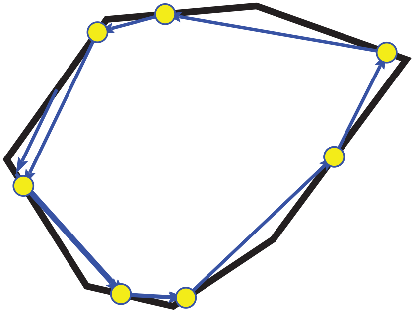
Proof. The only such edges will be edges for which both endpoints are reflex vertices or vertices inserted by Algorithm 1, because by Corollary 1, edges adjacent to other vertices of $P$ will be reachable by a safe action. Thus, planning in $G_{safe}$ is not complete: we cannot get everywhere safely, at least under this partitioning of $\partial P$ .

Figure 10 is an example where the edge $v_{10} v_{11}$ is not reachable via safe actions. Equivalently, node 10 in $G_{safe}$ has no incoming arcs.□

Fig. 10.

A polygon after Algorithm 1 and its safe bounce visibility graph $BV G_{safe}$ .

7.1.1. Constant strategy search

Despite a lack of complete reachability, we would like to have a tool to compute safe non-deterministic controllers of minimal complexity, for applications such as micro-scale robotics. Here, we show how to search for a constant fixed-angle bounce controller, where at every stage the robot executes a fixed-angle bounce in some range $\tilde{θ}$ . This is an extension of the controllers analyzed by Nilles et al. (2017) for regular polygons. We define the following functions.

mkBVG: Uses the visibility information generated in Algorithm 1 to generate the bounce visibility graph in $O (n^{4})$ time.

mkSafeBVG: Using Definition 7 and Proposition 2, we can create a safe roadmap, $G_{safe}$ , out of the bounce visibility graph by traversing all edges and removing edges with an empty $\tilde{θ}$ , and labelling the remaining edges with the interval of safe actions.

SearchConstantFixedStrats: performs breadth-first search from start to goal, starting with $\tilde{θ} = (0, π)$ and intersecting $\tilde{θ}$ with the safe action intervals along each path, terminating when the path reaches the goal state with non-zero $\tilde{θ}$ intervals. Returns the resulting constant controller $\tilde{θ}$ or that no such strategy is possible.

7.1.2. Examples

Here we provide an example of strategies that can be generated with different types of search in the safe bounce graph. We use an example environment consisting of two convex “rooms” connected with a corridor. The corridor does not have parallel sides, to make the problem more geometrically interesting.

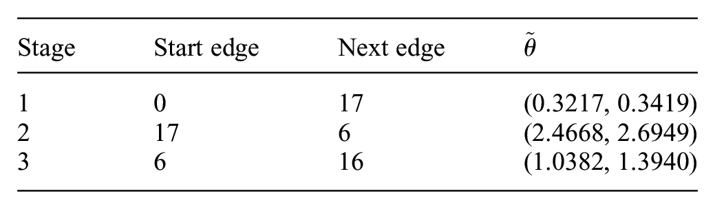
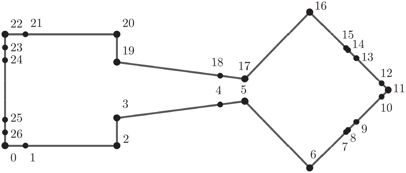
Using the SafeConstantFixedNavigate strategy in the environment shown in Figure 11, we can show that you cannot reach either “room” from the other under a constant strategy. An example feasible constant strategy was generated from edge $e_{5}$ to edge $e_{4}$ , with the action interval $\tilde{θ} = (0.0363, 0.1767)$ . This strategy causes the robot to bounce around the right room, and was validated by choosing random angles in the interval $(0.0363, 0.1767)$ as seen in Figure 12.

Fig. 11.

The example environment, discretized by Algorithm 1.

Fig. 12.

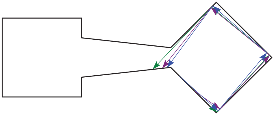
A trajectory from edge $e_{5}$ to edge $e_{4}$ , generated such that the same action set is used at each stage.

When we search for the path using the fewest number of transitions from a start point on segment $e_{0}$ to $e_{16}$ , we compute the plan

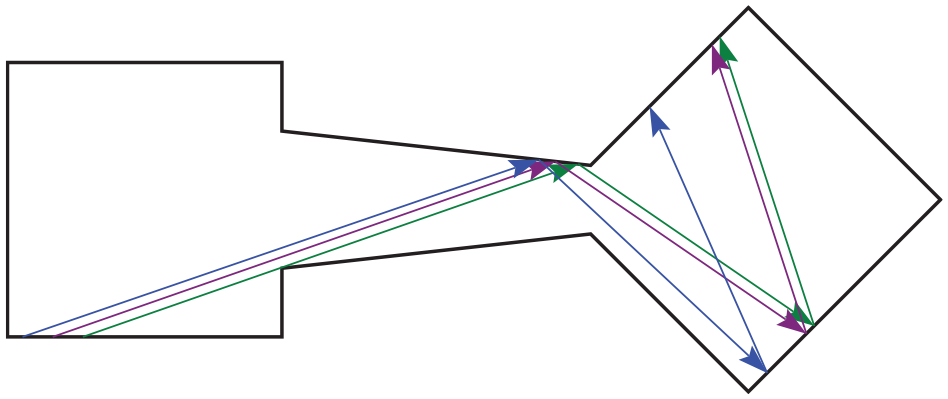
and we can see in Figure 13 that when a random start state is chosen in edge $e_{0}$ , and a random action from set $\tilde{θ}$ is chosen at each stage, that all trajectories successfully reach the goal.

Fig. 13.

A trajectory from edge $e_{0}$ to edge $e_{16}$ generated with the fewest bounces.

Stage	Start edge	Next edge	$\tilde{θ}$
1	0	17	(0.3217, 0.3419)
2	17	6	(2.4668, 2.6949)
3	6	16	(1.0382, 1.3940)

However, we notice that the action intervals at each stage are quite small, requiring accuracy from the robot of $0.02$ rad, or about $1.15 °$ . To address this and improve tolerance for uncertainty, there are several options. For example, we can set a minimum uncertainty (size of action set) and search for paths until we find one with at least that size. We may also search for the path (of under a certain bounded number of transitions) with the largest minimum action set. Future work will also include using the contraction property of transitions directly in the planning process; the goal is to construct a plan that intrinsically reduces uncertainty in robot state to generate more robust plans. Figure 14 shows an example of such a sequence of transitions. The initial robot state (on the bottom edge of the polygon) is quite large, but shrinks through successive actions. This type of transition cannot be found by the current planner, but we are actively working on encoding this knowledge into the planner.

Fig. 14.

An example of how contraction properties can be used to control robot state uncertainty enough to navigate the robot through a narrow doorway with non-deterministic actions.

7.2. Patrolling

In Section 6.1, we detailed results on the existence and structure of convex limit cycles in convex polygons, as well as how cycles can be used in general to reduce uncertainty in robot position. However, when considering how to plan trajectories including cycles, it is important to note that there are exponentially many possible limit cycles (in the size of the polygon), even if we restrict our controller to a fixed bounce rule. The main reason for this is that a cycle may contain transitions which are not contraction mappings, as long as the overall contraction coefficient is less than one.

However, it is possible to take any given sequence of edges in a polygon and check whether the sequence admits a stable limit cycle, by searching over the bounce rules at each stage for rules that cause an overall contraction coefficient to be less than one and satisfy the geometric constraints. As more becomes understood about the structure and robustness of the limit cycles, we can begin to formalize robotic patrolling tasks as a search over possible cycles. Here, we outline the general form of the patrolling problem.

Definition 15. Given an environment $P$ , a set of possible starting states $S$ , and a sequence of edges of the environment $E = {e_{1}, \dots, e_{k}}$ , determine a strategy which causes the robot to enter a stable cycle visiting each edge of the sequence in order from any point in $S$ .

This task is related to the aquarium keeper’s problem in computational geometry (Czyzowicz et al., 1991). It may be solved by coloring nodes in the bounce visibility graph by which edge of $P$ they belong to, and then searching for cycles which visit edges in the correct order. If a cycle is contracting, it will result in a converging stable trajectory. Interesting open questions remain on how to incorporate other useful properties of a patrolling cycle, such as coverage of a space with certain sensors, or guarantees about detecting evaders while patrolling. We are also interested in how to use heuristics and approximate methods to more efficiently search for such cycles, because it is equivalent to the traveling salesman problem and is therefore NP-hard.

7.3. Reachability and environment characterization

Proposition 5 states that there exist simple polygons containing edges unreachable via safe actions from any other edge in $P'$ . At first glance, this appears to be a major flaw of the proposed approach. Here, we present results of our investigations into the scope and impact of this property of the discretization.

First we examine irregular star polygons, generated by a pseudorandom program (Ounsworth, 2015) that places vertices at random distances from the origin with random angular intervals between them. We use two heuristic parameters, irregularity and spikiness, to generate a range of these polygons. A larger irregularity parameter increases the range of random values for the angular distances between vertices, and a larger spikiness parameter increases the range of random values for the linear distance between vertices and the origin.

It is important to note that this family of polygons is “easy” for a visibility-based discretization, for the simple reason that there is at least one point in the polygon (the origin) that is visible to all boundary points. Related concepts such as the art gallery problem or link distance (Toth et al., 2017) can be used to quantify the “complexity” of a polygon in terms of visibility decompositions.

Figure 15 shows a heatmap of the proportion of unreachable area along the polygon boundary, averaged over ten random polygons for each pair of irregularity/spikiness parameters. We have also included representative examples from the extremes of the parameter space. The measure of the unreachable segments of the polygon boundary was found by first finding all the nodes of the safe bounce visibility graph with no incoming edges. 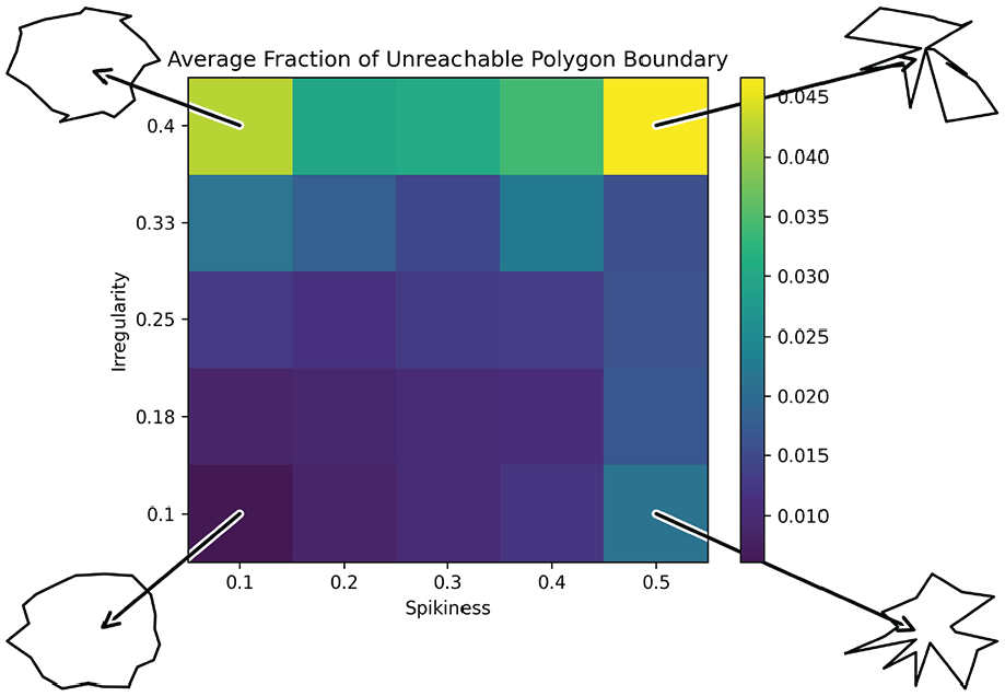These nodes correspond to segments in the discretized polygon $P'$ that cannot be reached from any other segments under safe actions. The fraction of unreachable polygon boundary was computed as the sum of the length of these unreachable segments divided by the total perimeter length of the polygon.

Fig. 15.

The fraction of the polygon that is unreachable under safe actions from any other starting segment. The results were computed for 10 random polygons at each pair of (spikiness, irregularity) parameters.

Nearly all polygons contain at least some fraction of the boundary that is unreachable under safe actions; however, this fraction is often very small. In all cases, an average of at least 95% of the polygon is reachable via safe action from somewhere else in the polygon under our discretization. As expected, the most spiky and irregular polygons contain the highest proportion of unreachable boundary (though still usually less than 5%).

7.4. Connectivity

Of course, this simple measure does not take into account overall connectivity of the discretized boundary space; however, the bounce visibility graph naturally allows for further inquiries into the connectivity of the environment under our discretization. The strongly connected components of the safe bounce visibility graph represent a partition where in each subgraph, every boundary segment can reach every other boundary segment. In addition, the number of weakly connected components in the safe bounce visibility graph indicates the number of boundary regions that cannot reach each other under safe actions. It is possible that for some environments, subsets of the space are entirely unreachable from each other. The directed transitions between strongly connected components indicate which transitions are not reversible.

The number of strongly and weakly connected components in the safe bounce visibility graph were analyzed for the same family of randomly generated polygons described in the previous section. Results can be seen in Figure 16. The results indicate that irregularity and spikiness have a strong influence on connectivity of the planning roadmap, especially for strongly connected components. However, the number of weakly connected components is low even when the number of strongly connected components is high. This indicates that while our planning method does not result in complete reachability (cannot reach any goal from any start), overall connectivity of the space is still good. Indeed, these results raise the possibility that our planner may also be well-suited as a tool to analyze and design environments for resource-constrained robots that use bouncing strategies as their motion primitive. For example, it may be desirable to build an environment that “funnels” micro-swimmers into a desired region. The safe bounce visibility graph for such an environment should have exactly one weakly connected component along with a node or strongly connected component reachable from all possible starting states.

Fig. 16.

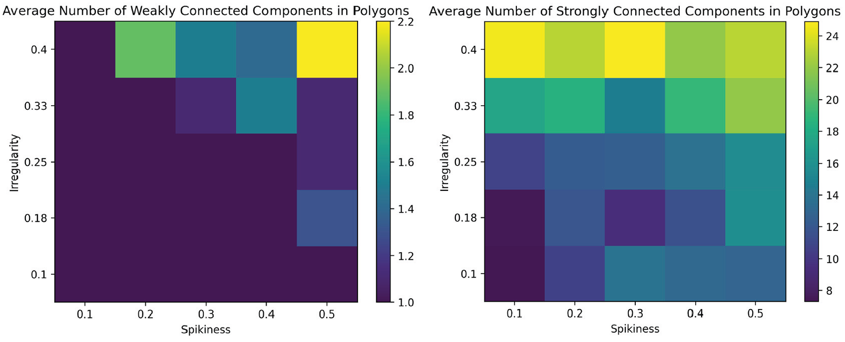
Average number of strongly and weakly connected components in the safe bounce visibility graph for random polygons. The results were computed for 10 random polygons at each pair of (spikiness, irregularity) parameters.

8. Open questions and future work

We have presented a visibility-based approach to reasoning about paths and strategies for a class of mobile robots. We are moving toward understanding non-deterministic control of such robots; however, many open questions remain.

8.1. Further characterization of complex environments

We have focused work here mainly on environments such as convex or star polygons, owing to the possibility for analytic results or the ease of parameterization. Of course, real-world applications must deal with different types of environments. In particular, future efforts will focus on “office” environments, remote environmental monitoring, and micro-fluidic applications. Challenges will include optimizations for scaling with respect to number of polygon edges and number of obstacles, and improving performance and guarantees for environments with challenging features such as long, narrow hallways or extremely irregular geometry.

8.2. Comparing bounce rules

Our approach can be used to compare different families of bounce strategies in a given polygon, by comparing the reachability of the transition systems induced by each strategy family. This would require either reducing the full bounce visibility graph given constraints on possible bounces, or constructing a more appropriate transition system. It is not clear the best way to analyze relative bounce rules, in which the outgoing angle of a robot after a collision is a function of the incoming angle.

8.3. Optimal strategies

Say we wish to find the strategy taking the robot from region $S$ to region $G$ with the maximum amount of allowed uncertainty in the bounce rules (the sum of the interval sizes of each action set along the path). We may also wish find sequences of transitions which are optimally contracting (maximally reduce uncertainty in robot position and effect of non-determinism). These problems can be framed as an optimization problem over the space of all transition function compositions, or could be solved with search algorithms such as $A^{*}$ with an appropriately discretized state space. Future work will address the best approach to finding such optimal strategies.

8.4. Localization

A localization strategy is a non-deterministic strategy that produces paths which reduce uncertainty in the robot’s position to below some desired threshold, from arbitrarily large starting sets. The use of limit cycles to produce localizing strategies has been explored by Alam et al. (2018), and it would be interesting to take a similar approach with our environment discretization.

8.5. Ergodic trajectories

We are interested in strategies that produce ergodic motion, where the robot’s trajectory “evenly” covers the state space. Measures of ergodicity have recently been used in exploration tasks (Miller et al., 2016). Chaotic dynamical systems have also been used directly as controllers for mobile robots (Nakamura and Sekiguchi, 2001).

Footnotes

Funding

The author(s) disclosed receipt of the following financial support for the research, authorship, and/or publication of this article: This work was supported by the NSF (grant numbers 1035345 and 1328018) and CONACyT (post-doctoral fellowship 277028).

ORCID iDs

Alexandra Q Nilles

Israel Becerra

References

Alam

Bobadilla

Shell

(2017) Minimalist robot navigation and coverage using a dynamical system approach. In: IEEE IRC.

Alam

Bobadilla

Shell

(2018) Space-efficient filters for mobile robot localization from discrete limit cycles. IEEE Robotics and Automation Letters 3(1): 257–264.

Allen

Burdick

Rimon

(2015) Two-finger caging of polygonal objects using contact space search. IEEE Transactions on Robotics 31(5): 1164–1179.

Anders

Kaelbling

Lozano-Perez

(2018) Reliably arranging objects in uncertain domains. In: 2018 IEEE International Conference on Robotics and Automation (ICRA). IEEE, pp. 1603–1610.

Aronov

Davis

Dey

Pal

Prasad

(1998) Visibility with multiple reflections. Discrete and Computational Geometry 20(1): 61–78.

Brunner

Mihalák

Suri

Vicari

Widmayer

(2008) Simple robots in polygonal environments: A hierarchy. In: Fekete

(eds) Algorithmic Aspects of Wireless Sensor Networks (ALGOSENSORS 2008) (Lecture Notes in Computer Science, Vol. 5389). Berlin: Springer, pp. 111–124.

Burridge

Rizzi

Koditschek

(1999) Sequential composition of dynamically dexterous robot behaviors. The International Journal of Robotics Research 18(6): 534–555.

Czyzowicz

, et al. (1991) The aquarium keeper’s problem. In: Proceedings of the Second Annual ACM-SIAM Symposium on Discrete Algorithms. Philadelphia, PA: SIAM.

Del Magno

Lopes Dias

Duarte

Gaivão

Pinheiro

(2014) SRB measures for polygonal billiards with contracting reflection laws. Communications in Mathematical Physics 329(2): 687–723.

10.

El Gindy

Avis

(1981) A linear algorithm for computing the visibility polygon from a point. Journal of Algorithms 2: 186–197.

11.

Erdmann

(1986) Using backprojections for fine motion planning with uncertainty. The International Journal of Robotics Research 5(1): 19–45.

12.

Erickson

LaValle

(2013) Toward the design and analysis of blind, bouncing robots. In: IEEE ICRA.

13.

Ghosh

(2007) Visibility Algorithms in the Plane. Cambridge: Cambridge University Press.

14.

Goldberg

(1993) Orienting polygonal parts without sensors. Algorithmica 10: 201–225.

15.

Granas

Dugundji

(2003) Elementary Fixed Point Theorems. New York: Springer, pp. 9–84.

16.

Lewis

Feshbach

O’Kane

(2018) Guaranteed coverage with a blind unreliable robot. In: 2018 IEEE/RSJ International Conference on Intelligent Robots and Systems (IROS). IEEE, pp. 7383–7390.

17.

Lewis

O’Kane

(2013) Planning for provably reliable navigation using an unreliable, nearly sensorless robot. The International Journal of Robotics Research 32(11): 1342–1357.

18.

Ardekani

(2014) Hydrodynamic interaction of microswimmers near a wall. Physical Review E 90(1): 013010.

19.

Lozano-Perez

Mason

Taylor

(1984) Automatic synthesis of fine-motion strategies for robots. International Journal of Robotics Research 3(1): 3–24.

20.

Lozano-Pérez

Wesley

(1979) An algorithm for planning collision-free paths among polyhedral obstacles. Communications of the ACM 22(10): 560–570.

21.

Lynch

Mason

(1995) Pulling by pushing, slip with infinite friction, and perfectly rough surfaces. The International Journal of Robotics Research 14(2): 174–183.

22.

Markarian

Pujals

Sambarino

(2010) Pinball billiards with dominated splitting. Ergodic Theory and Dynamical Systems 30: 1757–1786.

23.

Mason

(1985) The mechanics of manipulation. In: Proceedings IEEE International Conference on Robotics and Automation, pp. 544–548.

24.

Mayya

Pierpaoli

Nair

Egerstedt

(2019) Localization in densely packed swarms using interrobot collisions as a sensing modality. IEEE Transactions on Robotics 35(1): 21–34.

25.

Miller

Silverman

MacIver

Murphey

(2016) Ergodic exploration of distributed information. IEEE Transactions on Robotics 32(1): 36–52.

26.

Nakamura

Sekiguchi

(2001) The chaotic mobile robot. IEEE Transactions on Robotics and Automation 17(6): 898–904.

27.

Nilles

Becerra

LaValle

(2017) Periodic trajectories of mobile robots. Proceedings of IROS.

28.

Nilles

Ren

Becerra

LaValle

(2018) A visibility-based approach to computing nondeterministic bouncing strategies. In: Workshop on the Algorithmic Foundations of Robotics (WAFR).

29.

O’Rourke

Streinu

(1998) The vertex-edge visibility graph of a polygon. Computational Geometry: Theory and Applications 10(2): 105–120.

30.

Ounsworth

(2015) Algorithm to generate random 2D polygon. Mathematics Stack Overflow. Available at: https://stackoverflow.com/questions/8997099/algorithm-to-generate-random-2d-polygon (accessed 23 January 2021).

31.

Prasad

Pal

Dey

(1998) Visibility with multiple diffuse reflections. Computational Geometry 10(3): 187–196.

32.

Sahin

Guvenc

(2007) Household robotics: autonomous devices for vacuuming and lawn mowing [applications of control]. IEEE Control Systems 27(2): 20–96.

33.

Siméon

Laumond

Nissoux

(2000) Visibility based probabilistic roadmaps for motion planning. Advanced Robotics 14(6): 477–493.

34.

Spagnolie

Wahl

Lukasik

Thiffeault

(2017) Microorganism billiards. Physica D: Nonlinear Phenomena 341: 33–44.

35.

Suri

Vicari

Widmayer

(2008) Simple robots with minimal sensing: From local visibility to global geometry. The International Journal of Robotics Research 27(9): 1055–1067.

36.

Szirmay-Kalos

Márton

(1998) Worst-case versus average case complexity of ray-shooting. Computing 61: 103–131.

37.

Tabachnikov

(2005) Geometry and Billiards. Providence, RI: American Mathematical Society.

38.

Toth

O’Rourke

Goodman

(2017) Handbook of discrete and computational geometry. Boca Raton, FL: Chapman and Hall/CRC.

39.

Whitney

(1977) Force feedback control of manipulator fine motions. Transactions of the ASME, Journal of Dynamical Systems, Measurement, and Control 99(2): 91–97.