
Abstract
This article develops a methodology that enables learning an objective function of an optimal control system from incomplete trajectory observations. The objective function is assumed to be a weighted sum of features (or basis functions) with unknown weights, and the observed data is a segment of a trajectory of system states and inputs. The proposed technique introduces the concept of the recovery matrix to establish the relationship between any available segment of the trajectory and the weights of given candidate features. The rank of the recovery matrix indicates whether a subset of relevant features can be found among the candidate features and the corresponding weights can be learned from the segment data. The recovery matrix can be obtained iteratively and its rank non-decreasing property shows that additional observations may contribute to the objective learning. Based on the recovery matrix, a method for using incomplete trajectory observations to learn the weights of selected features is established, and an incremental inverse optimal control algorithm is developed by automatically finding the minimal required observation. The effectiveness of the proposed method is demonstrated on a linear quadratic regulator system and a simulated robot manipulator.
Keywords
1. Introduction
Inverse optimal control (IOC), also known as inverse reinforcement learning, solves a problem of finding an objective (e.g., cost or reward) function to explain behavioral observations of an optimal control system (Kalman, 1964; Ng and Russell, 2000). Successful applications of IOC techniques are broad, including imitation learning (Abbeel et al., 2010; Kolter et al., 2008), where a learner mimics an expert by inferring an objective function from the expert’s demonstrations, autonomous driving (Kuderer et al., 2015), where human driving preference is learned and transferred to a vehicle controller, human–robot shared systems (Mainprice et al., 2015, 2016), where the intentionality of a human partner is estimated to enable motion prediction and smooth coordination, and human motion analysis (Jin et al., 2019; Lin et al., 2016), where principles of human motor control are investigated.
The most common strategy used in IOC is to parametrize an unknown objective function as a weighted sum of relevant features (or basis functions) with unknown weights (Abbeel and Ng, 2004; Englert et al., 2017;Mombaur et al., 2010; Ng and Russell, 2000; Ratliff et al., 2006; Ziebart et al., 2008). Different approaches have been developed to estimate the weights of the features given an observation of the system’s optimal trajectory over a complete motion horizon, i.e., a full trajectory observation. These methods cannot deal with the case when only incomplete trajectory observations are available, that is, only a portion/segment of the system’s trajectory within a small time interval of the horizon is available. A method capable of learning objective functions from incomplete trajectory data will be beneficial for multiple reasons: first, an observation of the system’s trajectory over a complete time horizon may not be accessible due to limited sensing capabilities, sensor failures, occlusions, etc.; second, the computational cost of existing IOC techniques based on full trajectory data may be large; and, third, learning objective functions from incomplete trajectory observations may help to address some other challenging problems such as learning time-varying objective functions (Jin et al., 2019), online motion prediction (Pérez-D’Arpino and Shah, 2015), and learning from human corrections (Bajcsy et al., 2018). Under these motivations, this article aims to develop a technique to enable learning an objective function only from incomplete trajectory observations.
1.1. Related work
Existing IOC methods can be categorized based on whether the forward optimal control problem needs to be computed within the learning process. The first category of existing works is based on a nested architecture, where the feature weights are updated in an outer loop while the corresponding optimal control problem is solved in an inner loop. Different methods of this type focus on different strategies to update the feature weights in the outer layer. Representative methods include (Abbeel and Ng, 2004), where the feature weights are updated towards matching the feature values of the reproduced optimal trajectories with the demonstrations, (Ratliff et al., 2006), where the feature weights are solved by maximizing the margin between the objective function value of the observed trajectories and the value of any simulated optimal trajectories, and (Ziebart et al., 2008), where the feature weights are optimized such that the probability distribution of system’s trajectories maximizes the entropy while matching the empirical feature values of demonstrations. These nested IOC methods have been successfully applied to humanoid locomotion (Park and Levine, 2013), autonomous vehicles (Kuderer et al., 2015), robot navigation (Vasquez et al., 2014), learning from human corrections (Bajcsy et al., 2017; Jin et al., 2020), etc. In (Mombaur et al., 2010), the weights are learned by minimizing the deviation of the reproduced optimal trajectory from the observed one; the similar methods have been applied to studying human walking (Clever et al., 2016) and arm motion (Berret et al., 2011).
A drawback of the nested IOC methods is the need to solve optimal control problems repeatedly in the inner loop, thus those methods usually suffer from huge computational cost. This motivates the second line of IOC methods, which seek to directly solve for the unknown feature weights. A key idea used in these methods is to establish optimality conditions which the observed optimal data must satisfy. For example, in (Keshavarz et al., 2011), the Karush–Kuhn–Tucker (KKT) (Boyd and Vandenberghe, 2004) optimality conditions are established, based on which the feature weights are then solved by minimizing a loss that quantifies the violation of such conditions by the observed data. (Puydupin-Jamin et al., 2012) apply such a KKT-based method to solve IOC problems and study the objective function underlying human locomotion. In (Johnson et al., 2013), Pontryagin’s minimum principle (Pontryagin et al., 1962) is utilized to formulate a residual optimization over the unknown weights. These methods have been applied successfully to the locomotion analysis (Aghasadeghi and Bretl, 2014; Puydupin-Jamin et al., 2012), walking path generation (Papadopoulos et al., 2016), human motion segmentation (Jin et al., 2019; Lin et al., 2016), etc. (Englert et al., 2017) proposed an inverse KKT method to enable a robot to learn manipulation tasks. Recently, along this direction, the recoverability for IOC problems has been investigated. For example, when an optimal control system remains at an equilibrium point, although its trajectory still satisfies the optimality conditions, it is uninformative for learning the objective function. This issue is discussed in (Molloy et al., 2018, 2016), where a sufficient condition for recovering weights from full trajectory observations is proposed.
Existing IOC techniques cited previously require a full observation of a system trajectory, that is, optimal trajectory data of the system states and inputs over a complete motion horizon. To the best of the authors’ knowledge, the IOC problems based on incomplete trajectory observations are rarely investigated. By an incomplete trajectory observation, we mean that the observed data is a segment or portion of the system trajectory within a small time interval of the horizon. We consider the objective learning using incomplete trajectory data mainly due to the following motivations. First, in certain practical cases, for example, owing to limited sensing, sensors’ failure, or occlusions, a full observation of system’s trajectory data may not be available. Second, although direct IOC methods improve the computation efficiency compared with the nested counterparts, the computational cost is still significant especially when handling complex systems with high-dimensional action/state space and long time horizons. Third, successfully learning objective functions only using incomplete trajectory data would potentially benefit for addressing many challenging problems such as identifying time-varying objective functions (Jin et al., 2019), learning from human corrections (Bajcsy et al., 2018), and online long-term motion prediction (Mainprice et al., 2016).
1.2. Contributions
This article develops a methodology to learn an objective function of an optimal control system using incomplete trajectory observations. The proposed key concept to achieve this goal is the recovery matrix, which is defined on any segment data of the system trajectory and a given candidate feature set. We show that learning of the objective function is related to the rank and kernel properties of the recovery matrix. Different from existing methods, the recovery matrix also captures the unseen future information in addition to the available data by an unknown costate variable, which is jointly estimated along with the unknown feature weights. By investigating the properties of the recovery matrix, the following insights to solving IOC problems are enabled:
(1) the rank of the recovery matrix indicates whether an observation of incomplete trajectory data is sufficient for learning the feature weights;
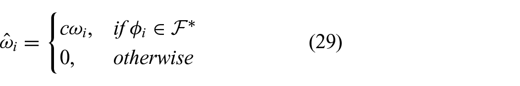
(2) additional observation data can contribute to learning the unknown objective function, or at least not degrade the learning; and irrelevant features can be identified;
(3) the IOC can be solved by incrementally incorporating the observation of each data point along the trajectory.
Based on the recovery matrix, an IOC approach based on incomplete trajectory observations is established, and an incremental IOC algorithm is developed by automatically finding the minimal required observation.
The structure of this article is as follows. Section 2 states the problem. Section 3 develops the recovery matrix and its properties. Section 4 presents the IOC method and algorithm using incomplete trajectory observations. Section 5 conducts numerical experiments, and Section 6 draws conclusions.
Notation
The column operator
2. Problem formulation
Consider an optimal control system with the following discrete-time dynamics and initial condition:

where the vector function

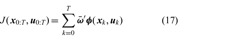
(locally) minimizes a cost function
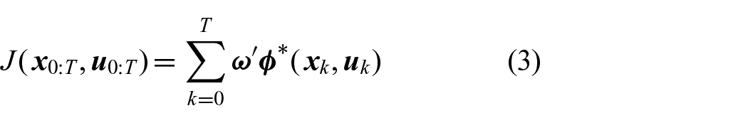
where

that is,
In IOC problems, one is given a relevant feature set
We have noted that existing IOC methods typically assume that the full trajectory data

which is a segment of
3. The recovery matrix
In this section, we introduce the key concept of the recovery matrix and show its relation to IOC process. Some properties of the recovery matrix are investigated to provide insights into the IOC process. Connections between the recovery matrix and existing methods are also discussed. The implementation of the recovery matrix is finally presented.
3.1. Definition of the recovery matrix
We first present the definition of the recovery matrix, then show its relation to the IOC problem solution, which is also the motivation of the recovery matrix.

with


Here,
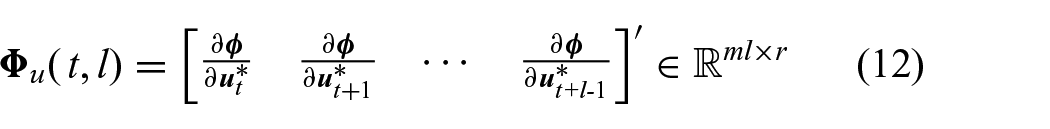
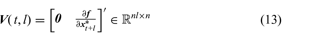
respectively.
Before showing a relationship between the recovery matrix and IOC, we impose the following assumption on the given candidate feature set
Assumption 1 requires that the relevant features

that is, the first s elements are from
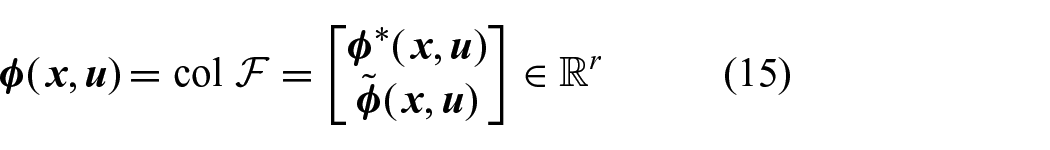
where

corresponding to (15), where
with the dynamics and initial condition in (1). Next, we distinguish the three optimal control settings, as described in the problem formulation, and then establish the relationship between the recovery matrix and the IOC problem solution.
Case I: Finite-horizon free-end optimal control. We first consider the optimal control setting with finite horizon T and free final state
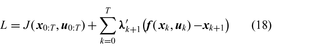
where
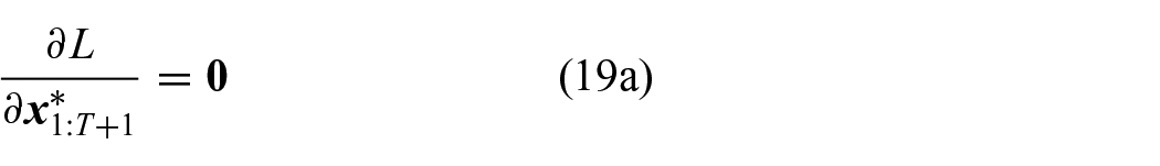
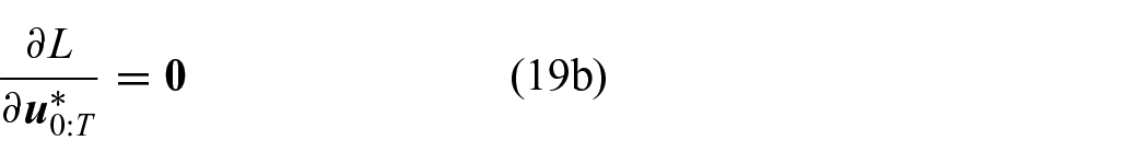
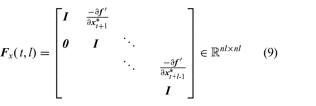
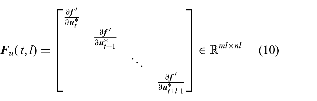
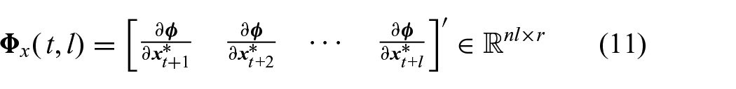
Based on the definitions in (9)–(13), Equations (19a) and (19b) can be written as


respectively, where in (20a),


respectively. For (21), we note that when
Case II: Finite-horizon fixed-end optimal control. We next consider the optimal control setting with a finite horizon T and a given fixed final state
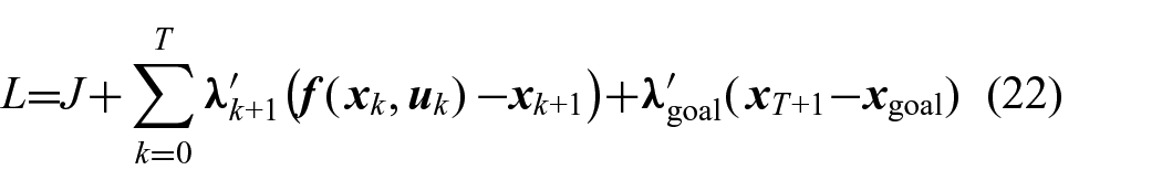
where the difference from (18) is that the term
Case III: Infinite-horizon optimal control. For the infinite-horizon optimal control setting, the optimal trajectory

where
Differentiating the Bellman optimality equation (23) on both sides with respect to
For any available trajectory segment
From the analysis, we conclude that, for any trajectory segment
By noting that
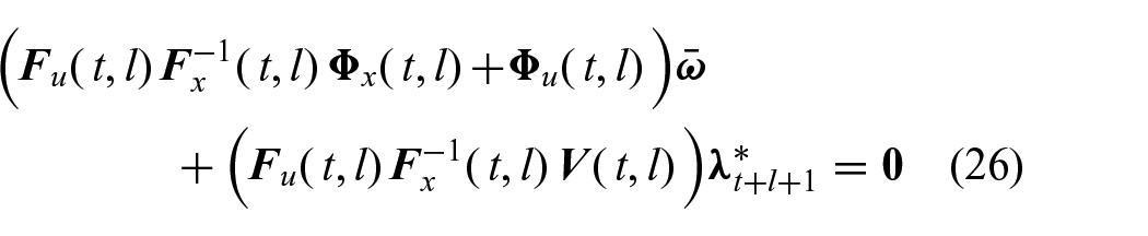
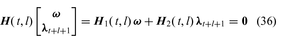
Considering the definition of the recovery matrix in (6)–(8), Equation (26) can be written as
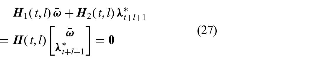
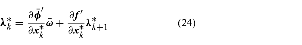
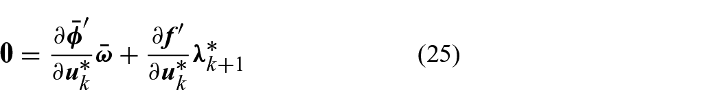
Equation (27) reveals that the weights
In IOC problems, in order to obtain an estimate of the unknown weights

then there exists a constant
and vector
Proof. Based on Equations (21), we note that for a trajectory segment
3.2. Properties of the recovery matrix
As the recovery matrix connects trajectory segment data to the unknown cost function, we next investigate the properties of the recovery matrix, which will provide us a better understanding of how the data and the selected features are incorporated in IOC process. We first present an iterative formula for the recovery matrix.
with
Proof. Please see Appendix A. □
The iterative property shows that the recovery matrix can be calculated by incrementally integrating each subsequent data point
The recovery matrix is defined on two elements: one is the segment data

if the new trajectory point
Proof. Please see Appendix B. □
We have noted in Theorem 1 that the rank of the recovery matrix is related to whether one is able to use segment data
The next lemma provides a necessary condition for the rank of the recovery matrix if the candidate feature set

always holds. If there exists another relevant feature subset

Proof. Please see Appendix C. □
Lemma 3 states that if a candidate feature set contains as a subset the relevant features under which the system trajectory
Combining Lemmas 2 and 3, we are able to show: under Assumption 1, (i) if the rank of the recovery matrix is less than
3.3. Relationship with prior work
We next discuss the relationship between the recovery matrix and existing IOC techniques (Aghasadeghi and Bretl, 2014; Englert et al., 2017; Johnson et al., 2013; Keshavarz et al., 2011;Molloy et al., 2018, 2016; Puydupin-Jamin et al., 2012). In those methods, an observation of the system’s full trajectory

where
Conversely, through the recovery matrix developed in this article, any trajectory segment
Comparing (35) with (36), we have the following comments.
(1) If we consider the segment

Comparing (37) with (35) we immediately obtain

Thus, the coefficient matrix
(2) However, as in (38), the coefficient matrix
(3) In addition to the capability of dealing with incomplete observation data, the recovery matrix can also provide insights and computational efficiency for solving IOC problems, as presented in Section 3.2. Such properties and advantages, however, cannot be achieved using the coefficient matrix
3.4. Implementation of rank evaluation
In practice, directly checking the rank of the recovery matrix is challenging due to: (i) data noise; (ii) near-optimality of demonstrations, i.e., the observed trajectory slightly deviates from the optimal one; and (iii) computational error. Thus, one can use the following strategies to evaluate the rank of the recovery matrix.
Normalization. When the observed data is of low magnitude, the recovery matrix may have the entries rather close to zeros, which may affect the matrix rank evaluation due to computing rounding error. Hence, we perform a normalization of the recovery matrix before verifying its rank,
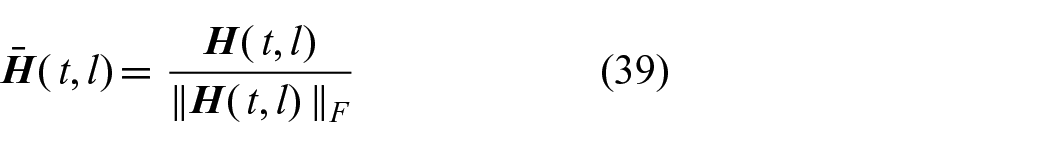
where

Rank index. As we are only interested in whether the rank of the recovery matrix satisfies
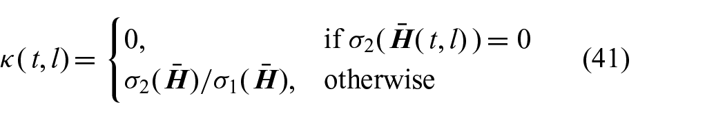
The condition

to decide whether
4. Proposed IOC approaches
Using the recovery matrix, in this section we develop the IOC techniques using incomplete trajectory observations to learn the cost function formulated in Section 2. Furthermore, we propose an incremental IOC algorithm by automatically finding the minimal required observation length.
4.1. IOC using incomplete trajectory observations
The following corollary states a method to use an observation of the incomplete trajectory to achieve a successful estimate of weights for given relevant features.

and a non-zero vector
Proof. As Corollary 1 is a special case of Theorem 1, by following a similar procedure as in proof of Theorem 1, we can show that there must exist a costate
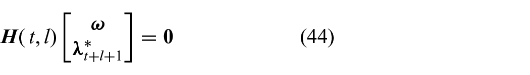
As the rank condition (43) holds, it follows that the nullity of
4.2. Incremental IOC algorithm
Combining Theorem 1 and the properties of the recovery matrix, one has the following conclusions: (i) as observations of more data points may contribute to increasing the rank of the recovery matrix (Lemma 2), which is however bounded from above (Lemma 3), thus the minimal required observation length

For any non-zero vector
Proof. Corollary 2 is a direct application of Theorem 1 and Lemmas 1–3. □
From Corollary 2, we note that starting from time t, the minimal required observation length
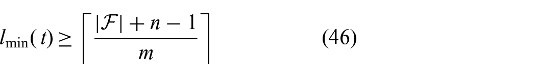
where ⌈·⌉ is the ceiling operation. Equation (46) implies that including additional irrelevant features to
In practice, directly applying Corollary 2 is challenging in the presence of data noise, near-optimality of trajectory, computing error, etc. Thus, we adopt the following strategies for implementation. First, (45) can be investigated based on the rank index (41) by checking (42) (the choice of
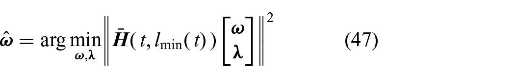
subject to
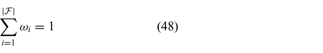
where ∥·∥ denotes the
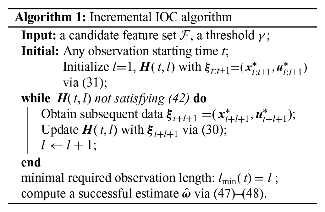
In sum, the implementation of the proposed incremental IOC approach in Corollary 2 is presented in Algorithm 1. Algorithm 1 permits arbitrary observation starting time, and the observation length is automatically found by checking the rank condition using (41) and (42). The algorithm can be viewed as an adaptive-observation-length IOC algorithm.
5. Numerical experiments
We evaluate the proposed method on two systems. First, on a linear quadratic regulator (LQR) system, we demonstrate the rank properties of the recovery matrix, show its capability of handling incomplete trajectory data by comparing with the related IOC methods, and demonstrate its capability to solve IOC for infinite-horizon LQR. Second, on a simulated two-link robot arm, we evaluate the proposed techniques in terms of observation noise, including irrelevant features, and parameter settings. Throughout evaluations, we quantify the accuracy of a weight estimate
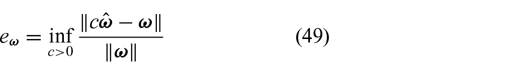
where ∥·∥ denotes the
5.1. Evaluations on LQR Systems
Consider a finite-horizon free-end LQR system where the dynamics is
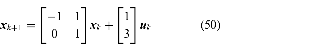
with initial

with the time horizon
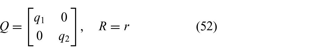
respectively. In the feature-weight form (3), the cost function (51) corresponds to the feature vector
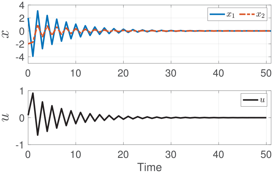
The optimal trajectory of a LQR system (50)–(51) using the weights
5.1.1. Minimal required observations for IOC
Based on the above LQR system, we here illustrate how the recovery matrix can be used to check whether incomplete trajectory data suffices for the minimal observation required for a successful estimation. Given the features
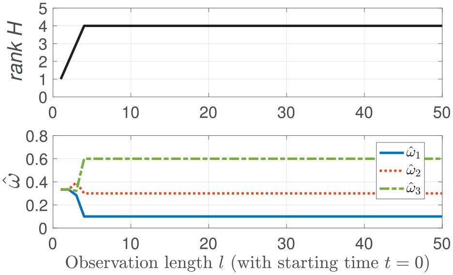
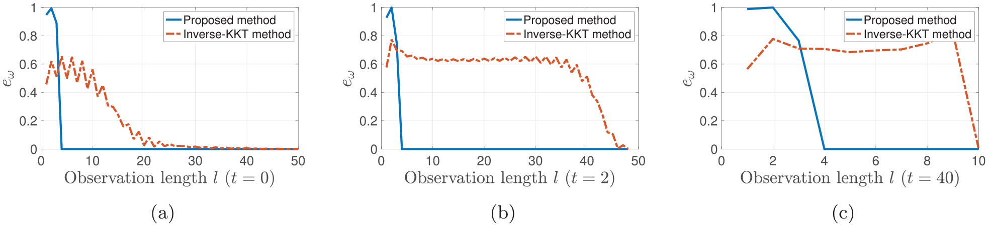
The rank of the recovery matrix and weight estimate when the observation starts at
As shown in the upper panel in Figure 2, including additional trajectory data points, i.e., increasing the observation length l (from 1), leads to an increase of the rank of the recovery matrix. When
5.1.2. Recovery matrix rank for additional observations
Based on the LQR system, we next show how additional observations affect the rank of the recovery matrix. Here, we vary the observation starting time t and use different candidate feature sets
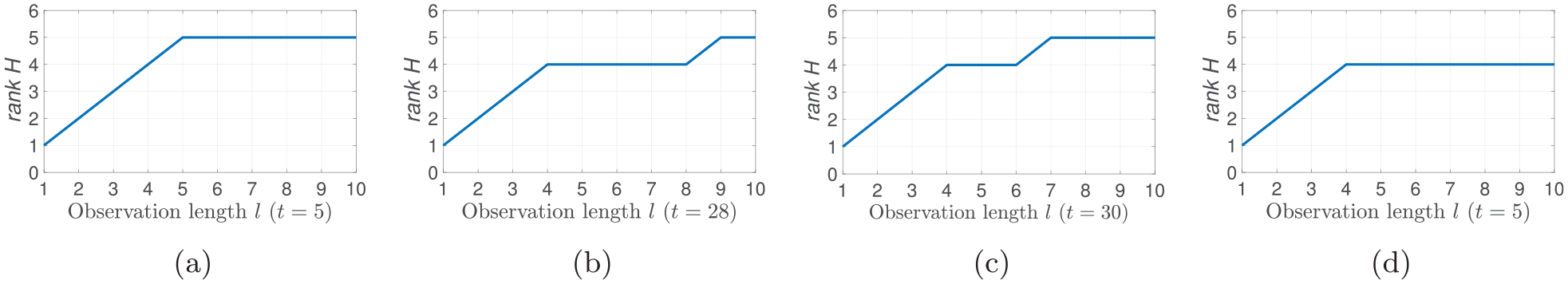
The rank of the recovery matrix versus the observation length l. For (a), (b), and (c), the observation starting time is at
(1) From Figure 3(a)–(c), we can see that additional observation (i.e., increasing observation length l) increases or maintains the rank of the recovery matrix, as stated in Lemma 2, and that continuously increasing the observation length will lead to the upper bound of the recovery matrix’s rank, as stated in Lemma 3.
(2) Comparing Figure 3(a) with Figure 3(d), we see that although the number of candidate features for both cases are the same, i.e.,
(3) Comparing Figures 3(a)–(c), we note that in some cases additional observations will not increase the rank of the recovery matrix, e.g., when the observation length is

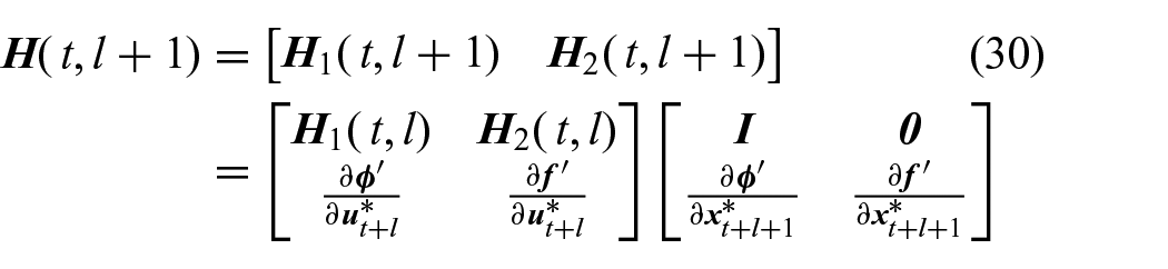
where the first two lines are directly from (30), and the last two lines are due to
5.1.3. Comparison with prior work
Here we demonstrate how the recovery matrix is able to solve IOC problems using incomplete observations. We show this by comparing with a recent inverse-KKT method developed in (Englert et al., 2017). The idea of the inverse-KKT method is based on the optimality equations similar to (35) using full trajectory data

subject to
As analyzed in Section 3.3, the coefficient matrix

Recall that this is because the LQR in (50)–(51) is a free-end optimal control system, as analyzed in Section 3.1,

with the proposed recovery matrix method
can show us how the unseen future data influences learning of the cost function.
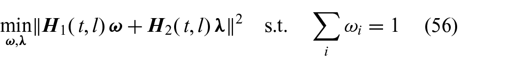
For the LQR trajectory in Figure 1, we use the feature set
Comparison between the inverse-KKT method (55) and proposed recovery matrix method (56) when given incomplete trajectory observation
(1) The inverse-KKT method is sensitive to the starting time of the observation sequence. When the observation starts from
(2) As we have analyzed in Section 3.3, the success of the inverse-KKT method requires that the given data
(3) In contrast, Figure 4 shows the effectiveness of using the recovery matrix to deal with incomplete observations. The proposed method guarantees a successful estimate after a much smaller observation length (e.g., around
In sum, we make the following conclusions. First, existing KKT-based methods generally require a full trajectory, and cannot deal with incomplete trajectory data. Second, the proposed recovery matrix method addresses this by jointly accounting for unseen future information; and the recovery matrix presents a systematic way to check whether a trajectory segment is sufficient to recover the objective function and if so, to solve it only using the segment data. Third, existing KKT-based methods can be viewed as a special case of the proposed recovery matrix method when the segment data is the full trajectory.
5.1.4. IOC for Infinite-horizon LQR
We demonstrate the ability of the proposed method to solve the IOC problem for an infinite-horizon control system. We still use the LQR system in (50)–(51) as an example, but here we set the time horizon
In IOC, suppose that we observe an arbitrary segment from the infinite-horizon trajectory; here we use the segment data within the time interval
IOC results for infinite-horizon LQR system. The observation starting time is
5.2. Evaluation on a two-link robot arm
To evaluate the proposed method on a non-linear plant, we use a two-link robot arm system, as shown in Figure 6. The dynamics of the two-link arm (Spong and Vidyasagar, 2008: p. 209) moving in the vertical plane is

where

which can be further expressed in state-space representation

with the system state and input defined as
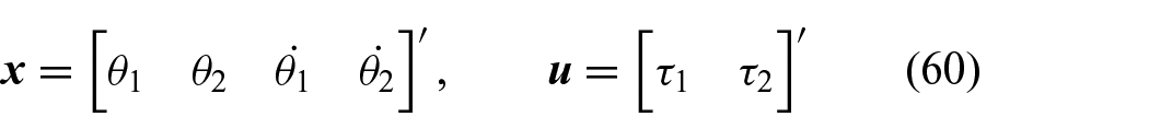
respectively. We consider the following finite-horizon fixed-end optimal control for the above robot arm system:
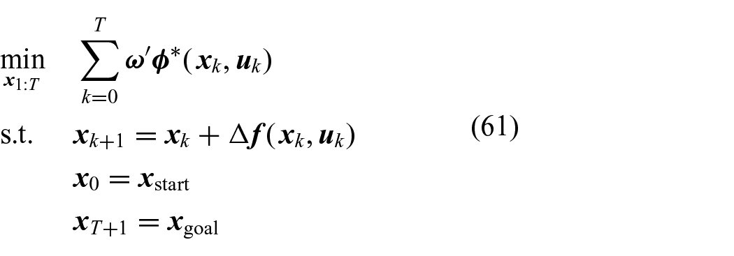
where
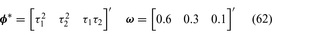
respectively. We solve the above optimal control system (61) using the CasADi software (Andersson et al., 2019) and plot the resulting trajectory in Figure 7.
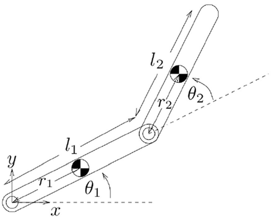
Two-link robot arm with coordinate definitions.
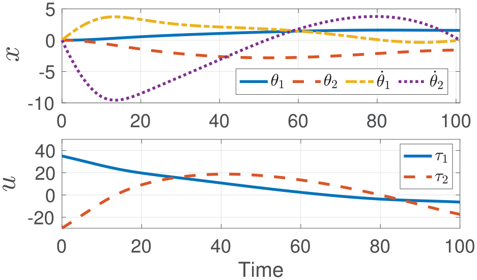
The optimal trajectory of the two-link robot arm optimal control system (61) and (62).
5.2.1. Minimal required observations for IOC
Based on the described robot arm system, we first show the use of the recovery matrix to check whether an incomplete trajectory observation suffices for the minimal observation required for successful IOC. As an example, in Figure 7, we set the observation starting time at
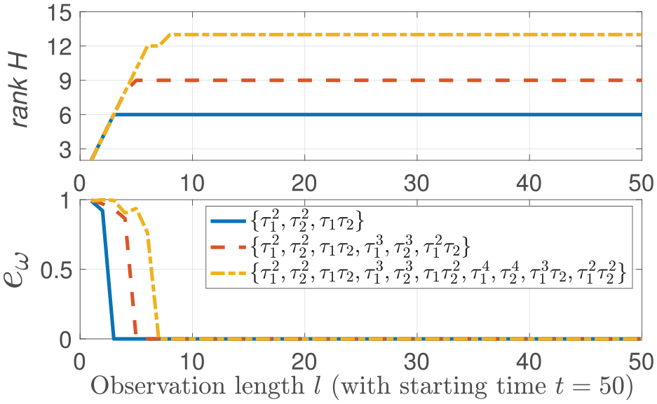
The rank of the recovery matrix and corresponding estimation error
Results in the upper panel of Figure 8 show that additional observations increase the rank of the recovery matrix. Once the additional observations lead to the upper-bound rank of the recovery matrix, i.e.,
5.2.2. Observation noise
We test the proposed incremental IOC approach (Algorithm 1) under different data noise levels. We add to the trajectory (both states and inputs) in Figure 7 Gaussian noise of different levels that are characterized by different standard deviations from
We set the observation starting time t at all time instants except for those near the trajectory end which cannot provide sufficient subsequent observation length. As an example, we present the experimental results for the case of noise level
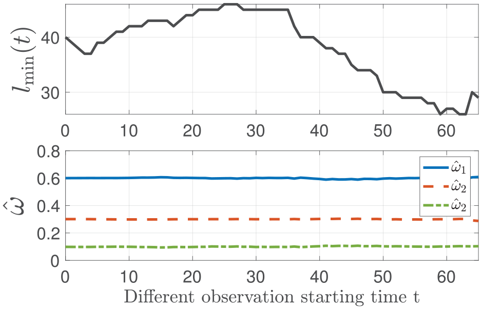
IOC by automatically finding the minimal required observation under noise level
From Figure 9, we see that the automatically found minimal required observation length
We summarize all results under different noise levels in Table 1. Here the minimal required observation length is presented in percentage with respect to the total horizon T. According to Table 1, under a fixed rank index threshold (here
Results of incremental IOC (Algorithm 1,
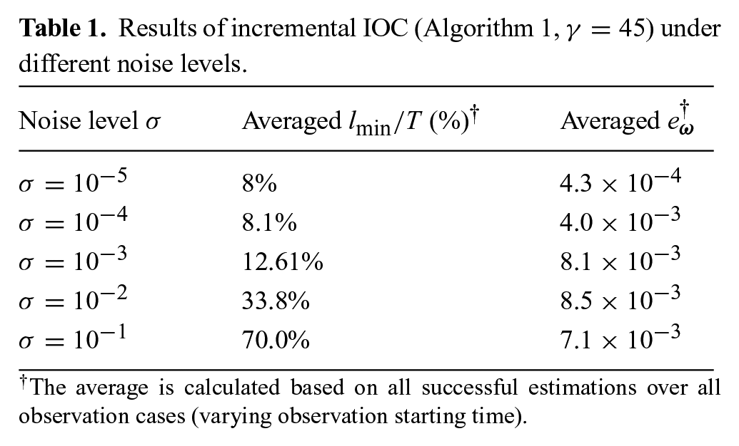
The average is calculated based on all successful estimations over all observation cases (varying observation starting time).
5.2.3. Presence of irrelevant features
We here assume that exact knowledge of relevant features is not available, and we evaluate the performance of Algorithm 1 given a feature set including irrelevant features. We add all observation data with Gaussian noise of
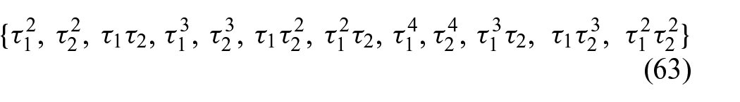
Algorithm 1 is applied the same way as in the previous experiment: by starting the observation at all time instants except for those near the trajectory end. We provide different candidate feature sets in the first column in Table 2, and for each case we compute the average of the minimal required observation length and the average of estimation error in (49). The results are summarized in second and third columns in Table 2.
Results of incremental IOC (Algorithm 1,
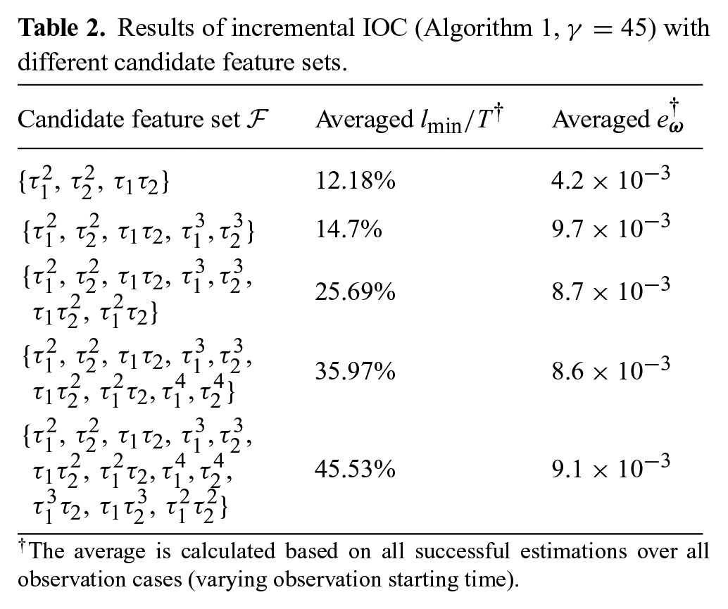
The average is calculated based on all successful estimations over all observation cases (varying observation starting time).
Table 2 indicates that on average, the minimal required observation length increases as additional irrelevant features are included to the feature set
5.2.4. Parameter setting
We now discuss how to choose the rank threshold
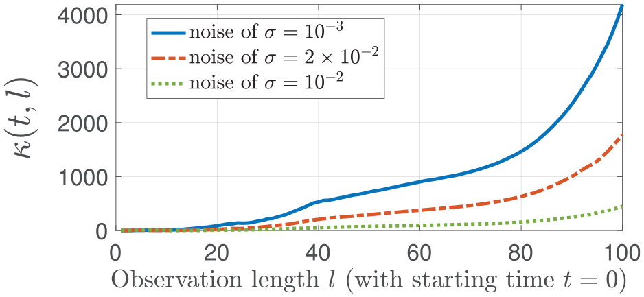
The rank index
From Figure 10, we can see that although
We add Gaussian noise
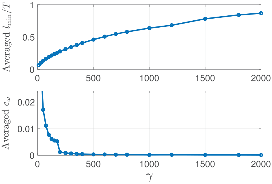
Averaged
6. Conclusions
This article has considered the problem of learning an objective function from an observation of an incomplete trajectory. To achieve this goal, we have developed the recovery matrix, which establishes a relationship between trajectory segment data and the unknown weights of given candidate features. The rank of the recovery matrix indicates whether an incomplete trajectory observation is sufficient for obtaining a successful estimate of the weights. By investigating the properties of the recovery matrix, we have further demonstrated that additional observations may increase the rank of the recovery matrix, thus contributing to enabling the successful estimation, and that the IOC can be processed incrementally. Based on the recovery matrix, a method for using incomplete trajectory observations to estimate the weights of specified features has been established, and an incremental IOC algorithm has been developed by automatically finding the minimal required observation.
Footnotes
Appendix A. Proof of Lemma 1
Consider the recovery matrix
and
Here
respectively. Here (66d) is based on the fact
with
Combining with (7)–(8), the above (67) becomes
Considering (66a)–(66d), we have
Finally joining (68) and (69) and writing them in the matrix form lead to (30).
When
Appendix B. Proof of Lemma 2
From Lemma 1, we have
If
Note that both (70) and the inequality (71) are independent of the choice of
Appendix C. Proof of Lemma 3
We first prove (33). Without losing generality, we consider the feature set in (14). For any trajectory segment
holds, where
We then prove (34). When another relevant feature subset
As
This completes the proof.
Funding
The author(s) disclosed receipt of the following financial support for the research, authorship and/or publication of this article: This research is partly supported by the ERC Consolidator Grant Safe data-driven control for human-centric systems under grant agreement 864686 at Chair of Information-oriented Control, Technical University of Munich.