Locally connected interrelated network: A forward propagation primitive

Abstract

End-to-end learning for planning is a promising approach for finding good robot strategies in situations where the state transition, observation, and reward functions are initially unknown. Many neural network architectures for this approach have shown positive results. Across these networks, seemingly small components have been used repeatedly in different architectures, which means improving the efficiency of these components has great potential to improve the overall performance of the network. This paper aims to improve one such component: The forward propagation module. In particular, we propose Locally Connected Interrelated Network (LCI-Net) – a novel type of locally connected layer with unshared but interrelated weights – to improve the efficiency of learning stochastic transition models for planning and propagating information via the learned transition models. LCI-Net is a small differentiable neural network module that can be plugged into various existing architectures. For evaluation purposes, we apply LCI-Net to VIN and QMDP-Net. VIN is an end-to-end neural network for solving Markov Decision Processes (MDPs) whose transition and reward functions are initially unknown, while QMDP-Net is its counterpart for the Partially Observable Markov Decision Process (POMDP) whose transition, observation, and reward functions are initially unknown. Simulation tests on benchmark problems involving 2D and 3D navigation and grasping indicate promising results: Changing only the forward propagation module alone with LCI-Net improves VIN’s and QMDP-Net generalisation capability by more than 3× and 10×, respectively.

Keywords

deep learning imitation learning reinforcement learning planning POMDP

1. Introduction

Stochastic planning requires stochastic models of the state transition, observation, and objective functions. However, such models are not always available, and attaining them can be difficult, especially when the dynamics of both the robot and the environment must be accounted for. To overcome this difficulty, end-to-end deep learning-based approaches for combined planning and learning have been proposed and have shown promising results. Many architectures have been proposed François-Lavet et al. (2019), Gupta et al. (2017), Karkus et al. (2017), Lee et al. (2018), Oh et al. (2015, 2017), Tamar et al. (2017), Wahlström et al. (2015). These different architectures often share common components and some of these components even appear repeatedly within a single network. Such components are akin to ‘primitives’ in planning, and therefore, we hypothesise that improving the efficiency of such components could substantially improve the capability of neural network–based combined planning and learning. This paper focuses on improving the efficiency of one such component: The forward propagation module – that is, the neural network component that propagates information on the basis of learned stochastic models of the state transition function.

A straightforward implementation of the forward propagation module often requires many parameters to be learned. Therefore, to reduce training time and data requirement, existing architectures simplify the models being learned. One commonly used approach is to transform states to abstract states and learn the transition models with respect to these abstract states, rather than states (e.g. François-Lavet et al., 2019; Oh et al., 2015; Wahlström et al., 2015). This is generally done via an auto-encoder: An encoder simplifies the current state into an abstract state, predicts the next abstract state via a fully connected layer, and then decodes the subsequent abstract state back into the original state. Transition from one abstract state to the next indeed requires a much smaller number of parameters to be learned. However, one needs to also learn the parameters for the auto-encoder. Moreover, the auto-encoder needs to be deep enough to generate a sufficiently small feature space, which generally increases the number of parameters to be learned.

Other architectures learn a state transition function with respect to the entire state space, but reduce the number of parameters to be learned by exploiting the fact that state transitions are generally local, and by assuming that they depend only on actions, rather than state–action pairs (e.g. Gupta et al., 2017; Karkus et al., 2017; Lee et al., 2018; Oh et al., 2017; Tamar et al., 2017). This is done via weight sharing in a convolution network, where the transition function for each action is represented as a kernel, whose size is much smaller than the size of the state space. This architecture substantially reduces the number of parameters to be learned but, is more constrained in its function representation.

To take the best of both worlds, in this paper, we propose a forward propagation module, called Locally Connected Interrelated Network (LCI-Net). Key to LCI-Net is a novel locally connected network layer with indirectly interrelated weights. It enables LCI-Net to exploit the locality property present in most transition functions and applies the learned transition probabilities to the original states, rather than abstract states, while learning a transition function that depends on pairs of abstract states and actions. LCI-Net is differentiable and is designed for multi-task learning, in the sense that LCI-Net learns a stochastic model of system’s dynamics for a multitude of scenarios at once.

LCI-Net is a simple module that can be plugged into various neural network architectures that require information propagation governed by learned transition functions, such as model-based reinforcement learning and Bayesian filtering. In this paper, we evaluate LCI-Net by applying it to the Value Iteration Network (VIN) Tamar et al. (2017) and QMDP-Net architectures. VIN is a neural network architecture that finds policies for Markov Decision Processes (MDPs) whose transition and reward functions are initially unknown and are learned from data in an end-to-end fashion, while QMDP-Net Karkus et al. (2017) is a counterpart of VIN for Partially Observable Markov Decision Processes (POMDPs) whose transition, observation, and reward functions are initially unknown. Specifically, we use LCI-Net to replace the Forward Propagation Module of VIN and QMDP-Net respectively. For QMDP-Net, LCI-Net is applied to both its planning and Bayesian filter modules. Since QMDP-Net’s Bayesian filter is the End-to-End learnable Histogram Filter (E2E-HF) Jonkowski and Brock (2017), our evaluation applies LCI-Net to the E2E-HF architecture too. We evaluate the performance of LCI-Net on various 2D and 3D navigation and grasping benchmarks, and evaluate the results of learning on problems of the same class but with much larger state spaces. Simulation results indicate that replacing only the forward propagation component of VIN and QMDP-Net with LCI-Net improves their generalisation capability by 3× and 10×, respectively.

LCI-Net was first presented in Collins and Kurniawati (2020). In this work, we have expanded the explanation and evaluation of LCI-Net to include extensive testing in two different neural network architectures for planning in MDPs and POMDPs. The trend of the results is similar in both cases.

2. Background and related work

2.1. Background

Although LCI-Net can be applied to various neural network architectures that require a forward propagation module, to make the explanation concrete, in this paper, we focus on applying LCI-Net to compute good MDP and POMDP policies when the underlying model is not known a priori.

Formally, an MDP Puterman (2014) is a decision-making framework for problems with non-deterministic action effects. It is described by a 5-tuple⟨S, A, T, R, γ⟩, where S is the set of states and A is the set of actions. At each step, an MDP agent is in some state s ∈ S, takes an action a ∈ A, and moves from s to state s^′ ∈ S according to a conditional probability distribution T (s, a, s^′) = P (s^′|s, a), called the transition probability. Prior to executing the action, the agent does not know the exact effect of its action, but once it performs the action, it can fully observe which state it is in. After each step, the agent receives a reward R (s, a). The solution to an MDP problem is then a mapping from states to actions, called policy π , that maximises the expected total reward, that is

V^{*} (s) = \max_{a \in A} [R (s, a) + γ \underset{J (s, a)}{\underset{⏟}{\sum_{s^{'} \in S} T (s, a, s^{'}) V^{*} (s^{'})}}]

(1)

where γ ∈ (0, 1) is a discount factor to ensure the optimisation is well defined.

A POMDP Kaelbling et al. (1998), Sondik (1971) is the partially observable version of an MDP. Similar to MDPs, in POMDPs, the exact effects of actions are not known exactly prior to execution. However, unlike MDPs, in POMDPs, the states are only partially observable, and hence are never known exactly.

Formally, a POMDP is described by a 7-tuple ⟨S, A, O, T, Z, R, γ⟩. In this paper, the context will make it clear whether one refers to a POMDP or an MDP, and therefore for simplicity, we use the same notation to describe the overlapping components of POMDPs and MDPs —that is, S refers to the set of states, A is the set of actions, T refers to the transition probability T (s, a, s^′) = P (s^′|s, a), R refers to the reward the agent receives at the end of each step, and γ refers to the discount factor. Due to partial observability, a POMDP definition has two additional components: The set of observations, denoted as O, and the observation function Z (s^′, a, o) = P (o|s^′, a) that represents uncertainty in perception.

At each step, the agent is in some hidden state s ∈ S, takes an action a ∈ A, and moves from s to state s^′ ∈ S according to a conditional probability distribution T (s, a, s^′) = P (s^′|s, a), called the transition probability. The current state s^′ is then partially revealed via an observation o drawn from a conditional probability distribution Z (s^′, a, o) = P (o|s^′, a) that represents uncertainty in sensing. After each step, the agent receives a reward R (s, a), if it takes action a from state s. Due to uncertainty in both the effects of actions and observations perceived, a POMDP agent never knows its exact state, and represents this uncertainty as distributions over states, called beliefs, and denoted as b ∈ B. The solution to a POMDP problem is then a mapping from beliefs to actions, called policy π that maximises the expected total reward, that is

\begin{matrix} V^{*} (b) = \max_{a \in A} [\sum_{s \in S} R (s, a) b (s) + γ \\ \sum_{o \in O} P (o | b, a) V^{*} (τ (b, a, o))] \\ = \max_{a \in A} \sum_{s \in S} R (s, a) b (s) + γ \sum_{o \in O} \sum_{s^{'} \in S} \sum_{s \in S} b (s) Z (s^{'}, a, o) \underset{J_{int} (b, a)}{\underset{⏟}{T (s, a, s^{'}) V^{*} (τ (b, a, o))}}] \end{matrix}

(2)

where τ(b, a, o) is the belief after action a ∈ A is applied to b and observation o ∈ O is perceived, computed as

τ (b, a, o) (s^{'}) = η Z (s^{'}, a, o) \underset{b_{i n t} (s^{'})}{\underset{⏟}{\sum_{s \in S} T (s, a, s^{'}) b (s)}}

(3)

where η is a normalisation factor.

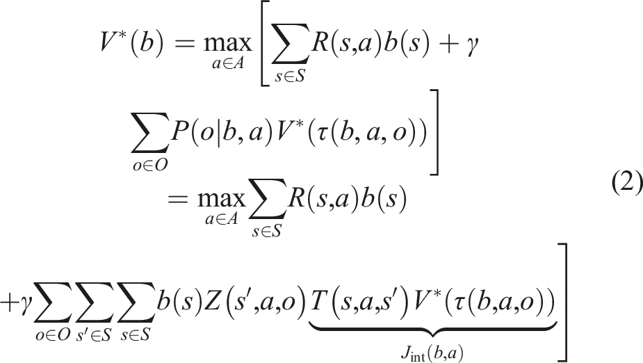
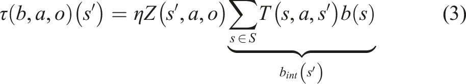
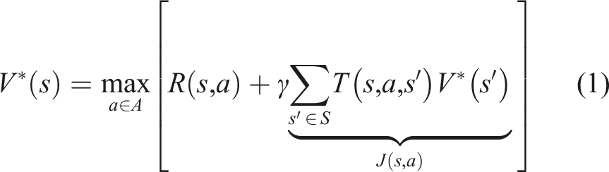
When the transition, observation, and/or reward functions are a priori unknown, one can compute an MDP or POMDP policy while learning the model, which can be formulated as an end-to-end reinforcement learning or imitation learning problem. LCI-Net can be applied as the forward propagation module, that is, J (s, a), J_int (b, a), and b_int (s^′) in equations (1), (2), and (3), respectively, in the mentioned learning approaches. In this paper, we apply LCI-Net to imitation learning.

2.2. Related work

Recently, there has been a growing body of works that apply deep learning through model-free approaches to solve large scale MDPs and POMDPs when the model is not fully known. The work in Hausknecht and Stone (2015), for instance, implemented a variation of DQN Mnih et al. (2015) which replaces the final fully connected layer with a recurrent LSTM layer to solve partially observable variants of Atari games. The work in Mirowski et al. (2016) applied convolutional neural networks with multiple recurrent layers for the task of navigating within a partially observable maze environment. The learned policy is able to generalise to different goal positions within the learned maze, but not to previously unseen maze environments.

However, more recently, success has been achieved with methods that embed specific computational structures representing a model and algorithm within a neural network and training the network end-to-end, a hybrid approach which has the potential to combine the benefits of both model-based and model-free methods. For instance, Tamar et al. (2017) developed VIN, a differentiable approximation of value iteration embedded within a convolutional neural network to solve fully observable Markov Decision Process (MDP) problems in discrete space. The work in Van der Pol et al. (2020) incorporate structures from group symmetries to solving MDP using neural network, while Okada et al. (2017) implemented a network with specific embedded computational structures to address the problem of path integral optimal control with continuous state and action spaces. These works focus only on cases where the state is fully observable.

By combining the ideas in the above work with recent work on embedding Bayesian filters in deep neural networks Haarnoja et al. (2016), Jonkowski and Brock (2017), Karkus et al. (2018), one can develop neural network architectures that combine model-free learning and model-based planning for POMDPs. For instance, Shankar et al. (2016) implemented a network which implements an approximate POMDP algorithm based on Q_MDP Littman et al. (1995) by combining an embedded value iteration module with an embedded Bayesian filter. Modules are trained separately, with a focus on learning transition and reward models over directly learning a policy. More recently, Karkus et al. (2017) developed QMDP-Net, which implements a Q_MDP approximate POMDP algorithm to predict approximately optimal policies for tasks in a parameterised domain of environments. Policies are learned end-to-end, focusing on learning an ‘incorrect but useful’ model which learns to optimise policy performance over model accuracy.

Recently, deep learning has been viewed as a new programming paradigm, called differentiable programming, where algorithms and data are implemented as differentiable neural network blocks Olah (2019), Karkus et al. (2019). Neural network ‘primitives’, such as a forward propagation module, can be viewed as one of the programming blocks, albeit one focused for stochastic planning. In this paper, we focus on improving the efficiency of this particular module.

Note that in this paper, the neural network layer we propose focuses only on a primitive computation, that is, forward propagation. This primitive can then be plugged in into multiple neural network modules for stochastic planning where the transition dynamics need to be learned. This is in contrast to neural network modules that aim to solve the entire planning problem, such as VIN and QMDP-Net for stochastic planning and MPNet Qureshi et al. (2019) for deterministic motion planning. We are of the opinion that optimising a primitive component alone is easier and will enable multiple different neural network modules for stochastic motion planning without a priori dynamic models to reap major benefits.

In prior works Haarnoja et al. (2016), Jonkowski and Brock (2017), Tamar et al. (2017), Shankar et al. (2016), Karkus et al. (2017), forward propagation has been accomplished via the use of convolutional layers, in which weights in a shared convolution kernel represent the probabilities of each possible relative change in position for each available action. Here, the channels of the convolution kernel represent available actions, while each position within the kernel represents a relative change in position from the previous state, with the centre position representing no change. A single set of kernel weights is learned via end-to-end learning, and applied universally to every state in the state space.

This forward propagation structure necessitates the use of a restricted transition model T (a, δs), where δs is a relative change in position within some local region of the current state s, as opposed to the complete transition model formulation T (s, a, s^′) introduced above. While this method of forward propagation is efficient, in that it greatly reduces the number of parameters required to be learned to represent transition dynamics and allows information learned about dynamics in one state to generalise to other states, it introduces the assumption that transition probabilities are independent of the original state. This restricts the expressiveness of the learned model, preventing key aspects of the dynamics of many systems from being represented.

This paper introduces an alternative formulation of the transition model and an accompanying module structure which relaxes this assumption, enabling significantly greater expressiveness while maintaining similar computational complexity to this existing approach.

The problem of learning a transition dynamics model in isolation has also been approached by a number of works. Lever et al. (2014) use online linear regression to transform states to an abstract feature space, building a compact representation incrementally using greedy feature selection to be used with a separate planning algorithm. Moerland et al. (2017) use deep generative models based on conditional variational inference to learn multi-modal transition dynamics models to be used by a planning algorithm. Sun et al. (2021) propose an algorithm for learning a dynamics model for multi-task learning settings based on transition templates, for use with a planning algorithm. These techniques are limited to conventional model-based learning in which learning and planning are separated, and are not applicable to the problem of end-to-end learning or the differentiable programming paradigm which are addressed by this paper.

3. LCI-Net

LCI-Net is a forward propagation layer that can be embedded into various neural network architectures that combine planning and model learning, such as François-Lavet et al. (2019), Gupta et al. (2017), Karkus et al. (2017), Lee et al. (2018), Oh et al. (2017), Tamar et al. (2017), Wahlström et al. (2015). Examples of the forward propagation component are J (s, a) in equation (1) for MDPs, and J_int (b, a) in equation (2) and b_int in equation (3) for POMDPs. Before presenting the details of LCI-Net, we will first describe the combined planning and learning problem.

3.1. Overview of the problem and LCI-Net

Let us consider the problem of learning a near optimal (PO) MDP policy, end-to-end, for acting in a parameterised set of stochastic scenarios: $W_{Θ} = {W (θ) | θ \in Θ}$ , where Θ is the set of all possible parameter values. We use similar notations to those used in Karkus et al. (2017), Tamar et al. (2017). Each parameter θ describes properties of the scenarios such as obstacle geometry and materials, position of static and dynamic obstacles, goal location, and initial belief distribution for a given task and environment. The problems of deciding how to act in the various scenarios in $W_{Θ}$ are defined as (PO) MDPs with a common state space $\underline{S}$ , action space $\underline{A}$ and observation space $\underline{O}$ but without a priori known transition, action, and observation functions.

A recent approach to solve the above problem is by using neural network to simultaneously learn the (PO) MDP models and perform value iteration using the learned model to compute the policy. In this paper, we focus on such a combined learning and planning approach too. We assume the neural network for solving the above problem embeds an internal model M(θ) = ⟨S, A, O, f_T (.|θ), f_Z (.|θ), f_R (.|θ)⟩, where S, A and O are the state space, actions space, and observation space respectively, which are manually specified, and constant across the set of tasks in the task domain. The notations f_T (.|θ), f_Z (.|θ), and f_R (.|θ) are the transition function, observation function, and reward function, respectively, and are represented by sub-networks which are trained end-to-end to maximise policy performance. LCI-Net focuses on one of these sub-networks.

Specifically, LCI-Net is a forward propagation layer that can be applied for a variety of purposes. For instance, to compute J (s, a) in the value function computation of MDPs (equation (1)) and to compute J_int (b, a) and b_int in the value function and belief update computations of POMDPs (equations (2) and (3)).

LCI-Net learns and propagates information via the transition function f_T (.|θ). It consists of two interrelated structures. The first structure represents the internal transition function, f_T (.|θ). Key in this structure is a representation suitable for robust learning, in the sense that the results of learning transfer across different tasks in the task domain and generalise beyond the training set. The second structure is designed to propagate information, such as state–action values (for value update) and beliefs (for belief update), through space over a single time step, in accordance to the transition function. These two structures are merged seamlessly within our proposed locally connected layer with indirectly interrelated weights. Details of these two structures are described in the following subsections, while the overall LCI-Net layer is illustrated in Figure 1,

Figure 1.

Transition operator based on locally connected layer with indirectly interrelated weights, shown with four shift operations, simplified to show propagation for only one action rather than all actions in the action space. Map Image is a component of θ representing properties of the environment. X(s) is a generic input which can represent value and belief.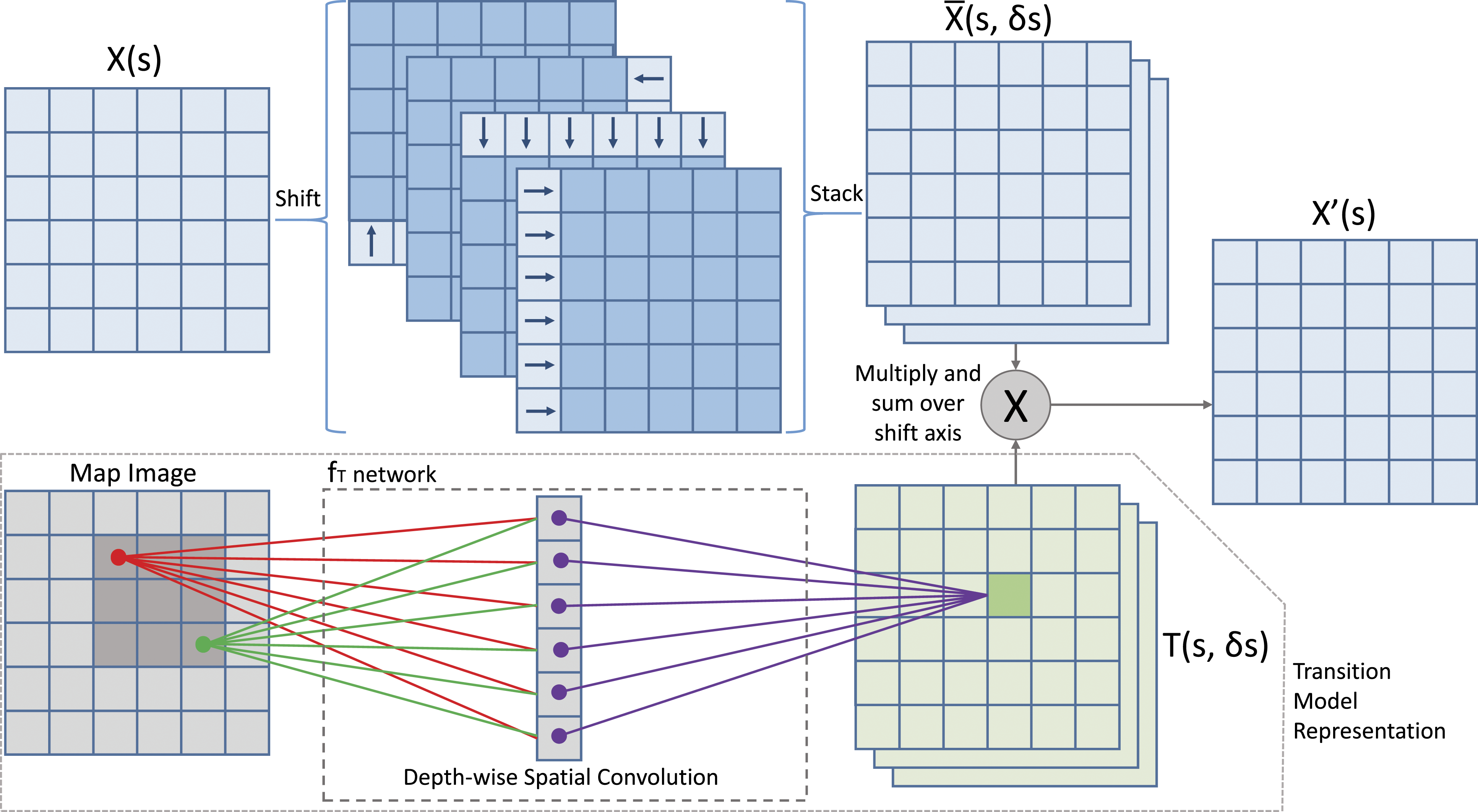

3.2. Learning the transition probability function

The transition function is parameterised by the current state s ∈ S, the action a ∈ A, and the subsequent state s^′ ∈ S. Therefore, a straightforward modelling of such a function requires |S|²|A| parameters to be learned, resulting in very large transition models for problems beyond trivial size. To reduce this learning complexity without sacrificing robustness, LCI-Net encodes known information about the problem’s structure in the neural network representation of the transition function.

To that end, LCI-Net approximates learning T (s, a, s^′) by learning T (s, a, δs), where δs ∈ D is a relative change in state within a local region D around the state s. This approximation is reasonable for many robotics problems where the support of the transition function T (s, a, s^′) is bounded within a relatively small local region around s, or the probability becomes very low outside of this small local region. However, naive implementation of the mentioned approximation requires learning parameters as many as |D‖S‖A|, where |D| is the size of the local region. Although the number of parameters to be learned has reduced from the original |S|²|A|, the size of S can be large.

To reduce the number learned parameters further, LCI-Net assumes locality and positional invariance. These assumptions mean that the transition probabilities from any state s depend only on h(s), a function which extracts the local features of s, with the property that T (s₁, a, δs) = T (s₂, a, δs) when h (s₁) = h (s₂). This assumption is appropriate because in general, only local environment features influence the effect of actions within a single time step. For instance, only surrounding obstacles (within the maximum distance an agent can traverse) matter to determine whether collision will occur within a single time step. Positional invariance is appropriate because the same pattern of local features can be expected to have the same effect on dynamics regardless of where the pattern occurs – any state where a wall blocks movement to the North produces a similar result when moving North is attempted.

Utilising the above assumptions, LCI-Net learns a set of kernel weights which allow the transition probabilities for each state–action pair to be predicted based on local environment features. It takes the scenarios $W (θ) \in W_{Θ}$ as inputs and uses a depth-wise spatial convolution network, with kernel width k to learn f_T (.|θ). The value k is set to be much smaller than |S|. For example, suppose the state space S is a 2D grid world and the support of T in each dimension of S is constrained to lie within r distance, where r is the maximum distance the agent can move in a single dimension of S within one time step, then k = 2r + 1. Each kernel weight in LCI-Net represents the probability P(S_t+1 = s + δs | h(s), A_t = a). Furthermore, the tensor produced by convolving θ with the learned kernel weights would be of dimensions (|S|, |A|, |D|). In the 2D example above, if the size of the scenario parameter θ is m × n, then the size of the tensor is (m, n, |A|, |D|). Each element of the tensor represents the conditional probability T(s, a, δs) = P(S_t+1 = s + δs | S_t = s, A_t = a). This representation means that LCI-Net learns a transition function that depends on the state, action, and subsequent state by learning only k²|D‖A| many parameters, with k < |S| being the number of kernel weights which is much smaller than the size of the state space.

Convolution layers have been used as a representation for learning transition functions in MDPs and POMDPs (e.g. Karkus et al., 2017; Tamar et al., 2017). However, LCI-Net’s approach is different from typical approaches today, where the learned kernel weights directly represent transition probabilities Haarnoja et al. (2016), Jonkowski and Brock (2017), Tamar et al. (2017), Shankar et al. (2016), Karkus et al. (2017). By using the approach above, LCI-Net relaxes assumptions on invariance of the transition function across the state space S into one that is invariant with respect to the local features of the states, without substantially increasing the number of parameters to be learned. Moreover, LCI-Net’s representation of the transition function uses the input and goal images, together with the reward and value function that are simultaneously learned, as it learns the transition function. This mechanism is in contrast to the transition function sub-network in VIN and QMDP-Net, where the input and goal images do not have a direct influence on the transition function being learned. As a result, LCI-Net is more robust to initial learning errors in the reward and value function.

Next, we must address the question of how the local region D is defined. D is composed of a set of directions specifying changes in position relative to the previous state. This set may be selected either as the complete set of all possible relative changes in position within some fixed distance, or be some restricted subset, for example, North, South, East and West in 2D space. This set of directions is common between all scenarios in $W_{Θ}$ . The type of set of directions is a hyper-parameter for the network.

An effective strategy for selecting sets of directions is estimating the maximum likelihood outcome of the transitions. For each action in the action space, the relative change in position which has the highest likelihood of resulting from performing the action should be included in the set of shift directions. For example, in the case where an agent performing a ‘drive’ action will move directly forward with probability α, and move in some other direction with probability 1−α, where α > 0.5, moving directly forward should be included in the shift direction set.

If a domain has transition behaviour which is multi-modal, then all movement directions with high likelihood should be included. While this selection depends on having some prior knowledge of the domain’s transition dynamics, estimating the most likely outcome of an action is much simpler than developing a complete ground-truth model of the system dynamics in many robotics applications, allowing the use of a restricted subset of shift directions to still be leveraged in domains without full a priori knowledge.

This strategy ensures that the directions in which transitions most frequently occur for all scenarios in $W_{Θ}$ are directly represented in the learned transition model, allowing values to be directly propagated through these directions.

3.3. Propagating information

To enable information such as state–action values or beliefs to be propagated via the learned transition probabilities in the form T(s, a, δs), LCI-Net first propagates the information without concern for probability, then scales the propagated information based on the learned transition probabilities.

Let X_t(s) be a function defined over the state space at time step t and state s ∈ S. In this work, X_t(s) may represent a set of state values V_t(s) or a belief distribution b_t(s). The transition operator of LCI-Net takes X_t(s) as input. This input is duplicated |A| times and stacked along a new axis to create channels corresponding to each possible action. For each channel (aka. each action in A), one shift operation is applied to the image for each direction δs ∈ D, where D is a set of directions (relative changes in position) – this set is the same as the set D of relative changes included in the support of the learned transition model T(s, a, δs). The resulting shifted images are stacked along an additional new axis. Let us denote this tensor as $\bar{X} (s, a, δ s)$ . In the case where |S| has two dimensions and size n × m, the shape of $\bar{X}$ is (n, m, |A|, |D|). Each element in this tensor represents propagation of information assuming the robot moves with probability one according to the shift direction δs. For instance, in value computation, the above tensor represents the expected total reward to arrive in state s after t steps if we assume the robot moves according to δs.

To account for uncertainty based on the learned transition model T(s, a, δs), LCI-Net performs element-wise multiplication of $\bar{X} (s, a, δ s)$ , followed by element-wise summation over the D-axis. The resulting tensor is the output X_t+1(s), representing the function X_t(s) propagated forward by one time step via the learned transition model.

The above network structure can be viewed as analogous to a locally connected network layer (in which locality is encoded, but weights are not shared), where the weights applied in each weighted sum are not independent trainable variables, but are instead provided by an external tensor, T(s, a, δs). This means that while the weights are not directly shared, they remain interrelated in that they are produced by f_T(.|θ), and so are each related to their local environment by the same weights (the kernel of f_T(.|θ)).

This new type of locally connected layer with indirectly interrelated weights structure provides a compromise which combines the superior generalisation capability of spatial convolution layers with the greater expressiveness of locally connected layers, while encoding algorithmic priors that are well suited to the problems of planning and state estimation. In the next subsection, we will elaborate the efficiency of LCI-Net in terms of the number of learned parameters.

3.4. Complexity analysis

To enable scaling to real world applications, it is essential that efficient time and space complexity are maintained. Compared to prior methods that use spatial convolution to learn the transition probabilities Haarnoja et al. (2016), Jonkowski and Brock (2017), Tamar et al. (2017), Shankar et al. (2016), Karkus et al. (2017), LCI-Net introduces only a small increase in the number of trainable variables and number of operations required, and has the same asymptotic complexity in terms of state and action space size.

Let r be the maximum range within which the agent can move in one time step. Equivalently, r is the maximum distance within which an environment feature such as an obstacle can influence the movement of the agent. This range corresponds to a convolution kernel width of k = 2r + 1. This kernel width applies to both the transition probability kernel in prior methods Tamar et al. (2017), Karkus et al. (2017), and the f_T(.|θ) network kernel in LCI-Net.

In LCI-Net, the number of channels is equal to the product of the size of the action space |A| and the number of shift directions, |D|, giving a total number of learnable parameters as k^dim|A||D|, where dim is the number of dimensions of the state space. Wlog, throughout the following discussions, we consider dim = 2. As a comparison, the number of channels in prior methods Tamar et al. (2017), Karkus et al. (2017) is equal to the number of available actions, which for 2D state spaces, gives a total of k²|A| parameters to be learned. Furthermore, in LCI-Net, no additional learnable parameters are introduced outside of the f_T(.|θ) component network. When D is selected to be the set of all possible shifts within the maximum range r, and the number of dimensions of S is fixed, the size of D is not directly dependent on the size of the number of states in S. This gives linear complexity in terms of the number of actions, and constant complexity in terms of the number of states, equivalent to that of prior methods.

In terms of the number of operations required, LCI-Net requires one multiplication and one addition for each combination of state, action, shift direction and kernel position. Additionally, a shift operation is required for each state. This gives a computational complexity proportional to (k²|A||D| + 1)|S|, where D can be considered constant when the number of spatial dimensions and maximum movement range are below a fixed maximum. As a comparison, prior methods Tamar et al. (2017), Karkus et al. (2017) require one multiplication and one addition for each combination of state, action and kernel position, resulting in a total number of operations proportional to k²|A||S|. This comparison shows that LCI-Net and prior methods Tamar et al. (2017), Karkus et al. (2017) have identical order of computational time complexity in terms of state and action space size.

In general, the size of |D| is linear in the transition range r and the number of dimensions, dim(S). However, scalability can be further improved by restricting D to a subset of the set of all possible shifts. Our experimental results on a diverse set of domains indicate that certain restrictions do not detrimentally affect policy performance or learning convergence speed.

4. Applying LCI-Net

In this work, we apply LCI-Net to replace the forward propagation module of an end-to-end decision-making system in fully observable scenarios (VIN Tamar et al., 2017) and partially observable scenarios (QMDP-Net Karkus et al., 2017).

4.1. Applying LCI-Net to VIN

The Value Iteration Network (VIN) implements value iteration as a recurrent neural network. This network consists of a repeating block structure, in which each block represents a single step of value iteration and blocks can be stacked to arbitrary depth to produce any desired planning horizon. Each value iteration block contains a forward propagation module that computes the intermediate value $V_{t + 1}^{'} (s, a) = \sum_{s^{'} \in S} T (s, a, s^{'}) V_{t} (s^{'})$ of equation (4). We replace this forward propagation module in each value iteration block with LCI-Net.

Each value iteration block takes as input a value image V_t(s|θ), and produces as output updated values based on one additional planning step, V_t+1 (s|θ), with the input to the first block, V₀(s|θ), taken from the prediction of the immediate reward associated with each s ∈ S provided by f_R(.|θ). In this application, LCI-Net takes V_t(s|θ) and produces $V_{t + 1}^{'} (s, a)$ . The reward image R(s, a) is then summed with $V_{t + 1}^{'} (s, a)$ to incorporate the immediate reward received at time step t + 1, yielding Q_t+1(s, a). V_t+1(s|θ) is then produced by selecting the action channel of Q_t+1 with the greatest expected return. Figure 2 illustrates this block.

Figure 2.

Value iteration network block. LCI-Net becomes its forward propagation module. Map image is a component of θ representing properties of the environment. Goal image is a component of θ representing properties of the task/objective.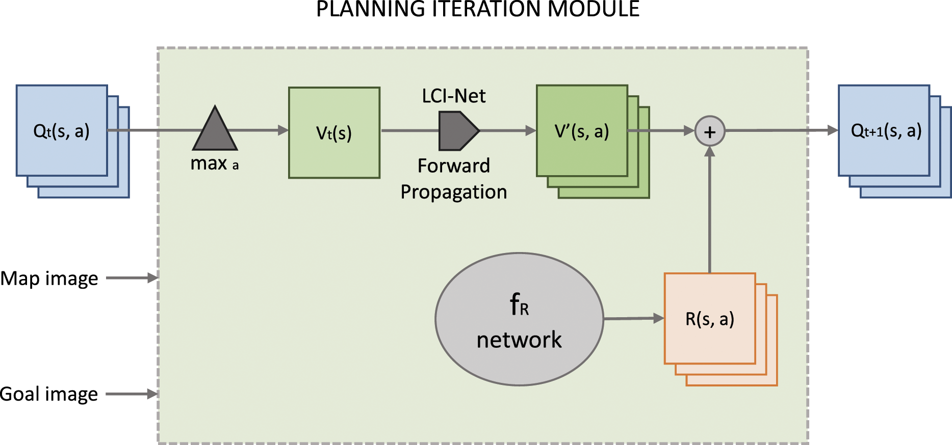

4.2. Applying LCI-Net to QMDP-Net

QMDP-Net’s overall architecture consists of two components: Planning and Belief Update. Both planning and belief update contain forward propagation operations. LCI-Net replaces the forward propagation module in both of those components.

The planning component approximates equation (2) using QMDP and is implemented similar to VIN. QMDP approximates equation (2) by assuming that the agent’s state becomes fully observable after the first step. More precisely, it computes $V^{*} (b) = \max_{a \in A} \sum_{s \in S} b (s) {R (s, a) + γ \sum_{s^{'} \in S} T (s, a, s^{'}) V^{*} (s^{'})}$ , where V*(s) is approximated via value iteration, that is, via iterative computation of

V_{t + 1} (s) = \max_{a \in A} [R (s, a) + γ \sum_{s^{'} \in S} T (s, a, s^{'}) V_{t} (s^{'})]

(4)

until t > t_max for a constant time limit t_max. QMDP-Net adopted the value iteration implementation of VIN Tamar et al. (2017), as described in the previous subsection. In this application, LCI-Net also replaces all forward propagation modules in the planning component of QMDP-Net, similar to the application of LCI-Net in VIN.

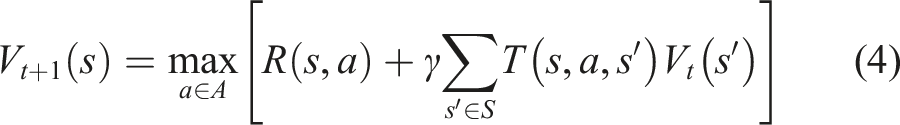
A POMDP agent maintains a belief, which is updated at each time step, as governed by equation (3). In QMDP-Net, belief update uses a neural network–based histogram filter, called E2E-HF. The forward propagation module is used in this filter to compute in the intermediate value $b_{t + 1}^{'} (s, a) = \sum_{s \in S} T (s, a, s^{'}) b (s)$ in equation (3). We replace this module in the belief update block with LCI-Net.

This belief update block takes a prior belief b_t, an action a_t and an observation o_t as input, and produces the updated belief b_t+1 as output, which is stored as the prior belief for the next action selection. In this application, LCI-Net is applied to the prior belief image to produce $b_{t + 1}^{'} (s, a)$ , the belief propagated forward by one time step after action a ∈ A is performed. This tensor is indexed based on the performed action a_t, with the channel corresponding to a_t retained, and all other channels discarded, giving b^′(s), the updated prior belief.

In parallel, the observation model Z(s|o) produced by the model component network f_Z(.|θ) is indexed based on the perceived observation o_t, with the channel corresponding to o_t selected to give Z(s), the likelihood of each state based on the perceived observation. b(s) and Z(s) are then multiplied and normalised to give the posterior belief b_t+1(s). Figure 3 illustrates this Belief Update component.

Figure 3.

Belief update network block. LCI-Net becomes its forward propagation module. Map image is a component of θ representing properties of the environment.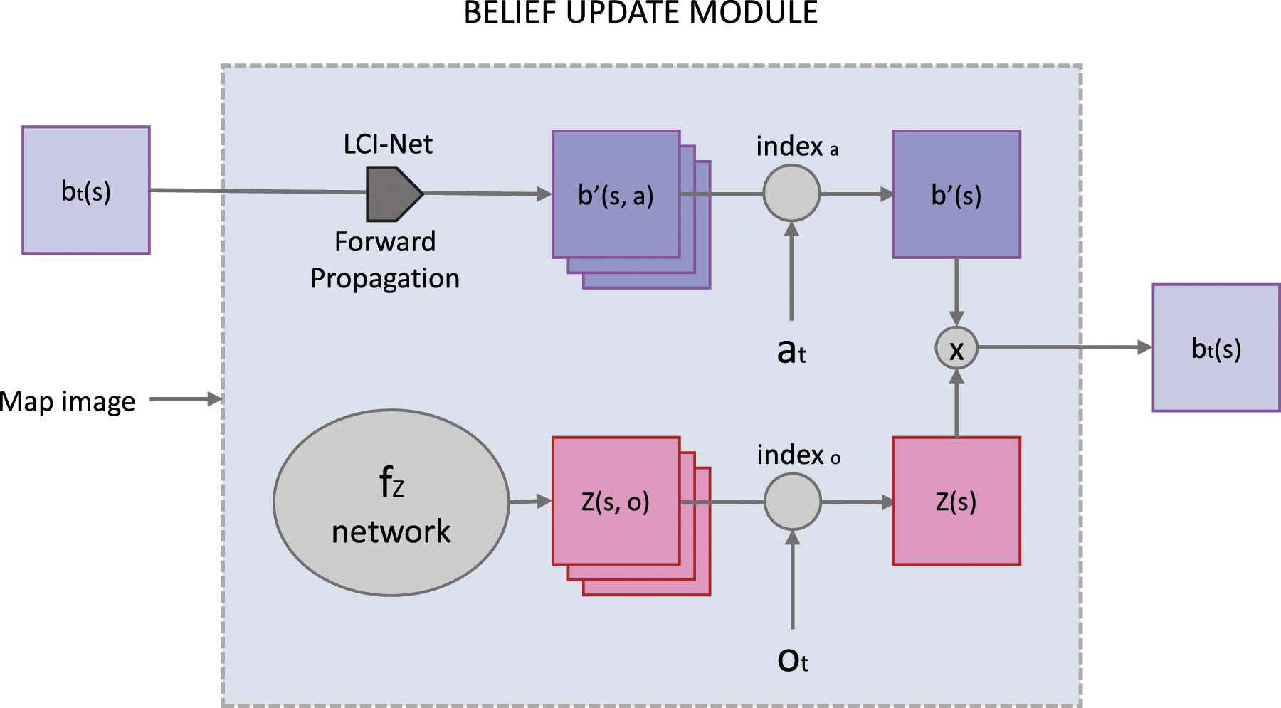

5. Experiments

5.1. Experimental setup

To evaluate the potential of LCI-Net in increasing the performance of combined learning and planning, we replace the forward propagation module of two different state-of-the-art deep learning for planning architectures – VIN Tamar et al. (2017) for fully observable planning, and QMDP-Net Karkus et al. (2017) for partially observable planning – and compared these modified variants of VIN and QMDP-Net (which we denote as LCI-Net for short) with the original VIN and QMDP-Net on a variety of fully observable (VIN) and partially observable (QMDP-Net) stochastic environments. Results of LCI-Net are based on an implementation developed on top of the software released by the authors of VIN and QMDP-Net, while VIN and QMDP-Net results are based on their released code (with VIN code modified for compatibility). The implementation of LCI-Net is available at https://github.com/RDLLab/lci-net

Both networks are trained via imitation learning using the same set of expert trajectories. In the fully observable case, expert trajectories are generated by solving ground-truth MDP models with value iteration. In the partially observable case, expert trajectories generated by applying the Q_MDP algorithm to manually constructed ground-truth POMDP models. Only trajectories where the expert was successful were included in the training set. The networks interact only with the expert trajectories and not with the ground-truth model. All hyper-parameters for both networks are set to match those used in the VIN and QMDP-Net experiments.

In all cases for both training and testing, the number of planning block repetitions is set to three times the largest dimension of the current environment. For example, for a 10 × 10, 30 repetitions of the planning block are used.

Training was conducted using GPU on an Nvidia GeForce RTX2070 GPU with 8 GB of dedicated memory. The GPU is installed in a machine equipped with an Intel Xeon Silver 4110 CPU (8 cores, 16 threads at 2.10 GHz) and 128 GB of system RAM. We tested the networks on four domain types:

5.1.1. 2D dynamic maze

A set of navigation problems in a maze environment with structure that mutates during run time in a way which qualitatively affects the optimum policy, designed to measure the robustness of a policy to dynamic environments. The robot must localise itself and navigate to the goal, while accounting for the possibility of environmental changes.

The robot is given a map of obstacle positions, a specified goal location, and initial belief distribution, which together form θ for each scenario in the set. No other environment information is given, and the POMDP model is not known a priori. At each time step, the robot selects a direction to move in: ‘move north’, ‘move south’, ‘move east’, ‘move west’ or ‘stay in position’. The outcomes of actions are probabilistic, with the support of the transition probabilities including the adjacent states in each of the four movement directions as well as the previous state. The agent moves in the chosen direction with probability p; all other outcomes have probability. Observations are received based on whether an obstacle is present in the adjacent cell in each of the ‘north’, ‘south’, ‘east’ and ‘west’ directions, with an independent fixed chance to receive an incorrect sensor reading for each direction.

To generate the dynamic maze layout, a maze is initially constructed using randomised Prim’s algorithm. The maze is divided into two partitions, with two cells from the border selected to be gates. At each time step, exactly one gate is open and the gates will swap from open to closed and vice versa with certain probability. During run time, the environment map provided to the agent is updated when a gate swap occurs. The start and goal position are selected such that a gate swap will cause the optimum solution to be qualitatively changed. Figure 4 illustrates an example. Two variations of this scenario are evaluated:

V1: The network is trained using only expert trajectories from a static maze navigation task. The environment image provided in θ shows only the positions of current free spaces and current obstacles, without special marking for open or closed gates.

V2: The network is trained using trajectories based on an expert which plans on a dynamic ground-truth POMDP model, allowing the expert to decide whether to wait for a nearby closed gate to open. The environment image received by the agent denotes the position of the gate which is currently closed. This may allow the agent to learn to intelligently decide whether to move or wait for the currently open gate to change. The open gate is not represented in the image.

Figure 4.

Example of a 9 × 9 dynamic maze environment in both possible gate states. Light grey represents an open gate, dark grey a closed gate. The agent must navigate from the red circle to the blue circle. The red line denotes the optimal trajectory.

The networks are trained on a set of 9×9 dynamic maze environments containing 2000 environments with five trajectories per environment, and evaluated on both 9×9 and 29×29 dynamic mazes. Evaluation results are based on 1250 trials composed of 50 environments, five trajectories per environment and five repetitions per trajectory. For all experiments, the action space, observation space, transition probabilities and observation probabilities are common between the training and testing environments.

5.1.2. 2D navigation with large scale realistic environments

A set of robot navigation problems in a general 2D grid setting with noisy state transitions and limited observations. The robot receives a map of obstacle positions, a specified goal location, and initial belief distribution, together forming θ. The POMDP model is not known a priori. At each time step, the robot selects a direction to move in, and receives a noisy observation indicating whether an obstacle is present in each direction. The networks are trained on artificial environments, with obstacle positions sampled at uniform random. Two different sizes of training environment are employed – 10×10 and 20×20. The 10 × 10 set contains 2000 environments with five trajectories per environment, while the 20 × 20 set contains 6000 environments with five trajectories per environment.

After training on the artificial environment set, evaluation is performed on environments modelled on the LIDAR maps from the Robotics Data Set Repository Howard and Roy (2003). The robot receives an environment floor plan, a specified goal position and a randomly initialised belief distribution. No other information or model is provided. Three different maps are evaluated in both deterministic and stochastic form, each with dimensions on the order of 100×100. For the deterministic case, evaluation results are based on 100 trials for each map. For the probabilistic case, results are based on 150 trials per map.

In the fully observable case, the action space includes movement in both axis aligned and diagonal directions, while in the partially observable case, the action space includes only axis aligned directions and remaining in the same position (e.g. to receive an additional observation when belief confidence is low). The outcome of actions is subject to probabilistic noise in both cases. The support of the transition probabilities includes the adjacent states in each of the allowed movement directions (eight directions for the fully observable case, four directions for the partially observed case) as well as the previous state. In both cases, the agent moves in its chosen direction with probability p, and all other outcomes have probability $\frac{1 - p}{| A | - 1}$ .

5.1.3. 3D navigation of multi-rotor drone

A set of three dimensional navigation problems representing the task of controlling autonomous multi-rotor drones with limited sensing through spaces with dense obstacles. State transitions are noisy, and observations are limited and unreliable. The drone is given a 3D model of obstacle positions, a specified goal location, and initial belief distribution as θ, and does not know the POMDP model a priori. The robot must localise itself and navigate to the goal. At each time step, the agent selects from the following actions: ‘move north’, ‘move south’, ‘move east’, ‘move west’, ‘move up’, ‘move down’ or ‘stay in position’. The support of the transition probabilities includes the adjacent states in each of these movement directions as well as the previous state. The agent moves in its chosen direction with probability p; all other outcomes have probability $\frac{1 - p}{| A | - 1}$ .

The networks are trained on a set of artificial 7 × 7 × 7 3D environments comprising of 6000 environments with five trajectories per environment, with evaluation performed on both 7 × 7 × 7 and 14 × 14 × 14. Evaluation results are based on 1250 trials composed of 50 environments, five trajectories and five repetitions.

5.1.4. 2D and 3D grasping

A robot gripper picks up randomly generated obstacles placed on a surface using a two-finger hand with observations received only via touch sensors mounted on the hand’s fingertips. The agent receives a 2D image or 3D model of the shape object to be grasped and an additional image or model indicating which parts of the object can feasibly be grasped for each scenario – together these form θ. The agent does not know its initial pose, and outcomes of transitions and sensor readings are probabilistic. We evaluate the networks on simplified variants of this task in both two and three dimensions. Figure 5 shows an example 3D grasping scenario. In the 2D case, the available actions are ‘move north’, ‘move south’, ‘move east’, ‘move west’ or ‘stay in position’. In the 3D case, the additional actions ‘move up’ and ‘move down’ are also available. The support of the transition probabilities includes the adjacent states in each of these movement directions as well as the previous state. In both cases, the agent moves in its chosen direction with probability p; all other outcomes have probability $\frac{1 - p}{| A | - 1}$ .

Figure 5.

Example of a 3D grasping task. Orange indicates the position of the grasping hand, and green and blue indicate an object to be grasped, where the blue areas are feasible grasp points. The left image shows a possible initial pose for the grasping hand, while the right image shows the hand grasping at feasible grasp point on the object.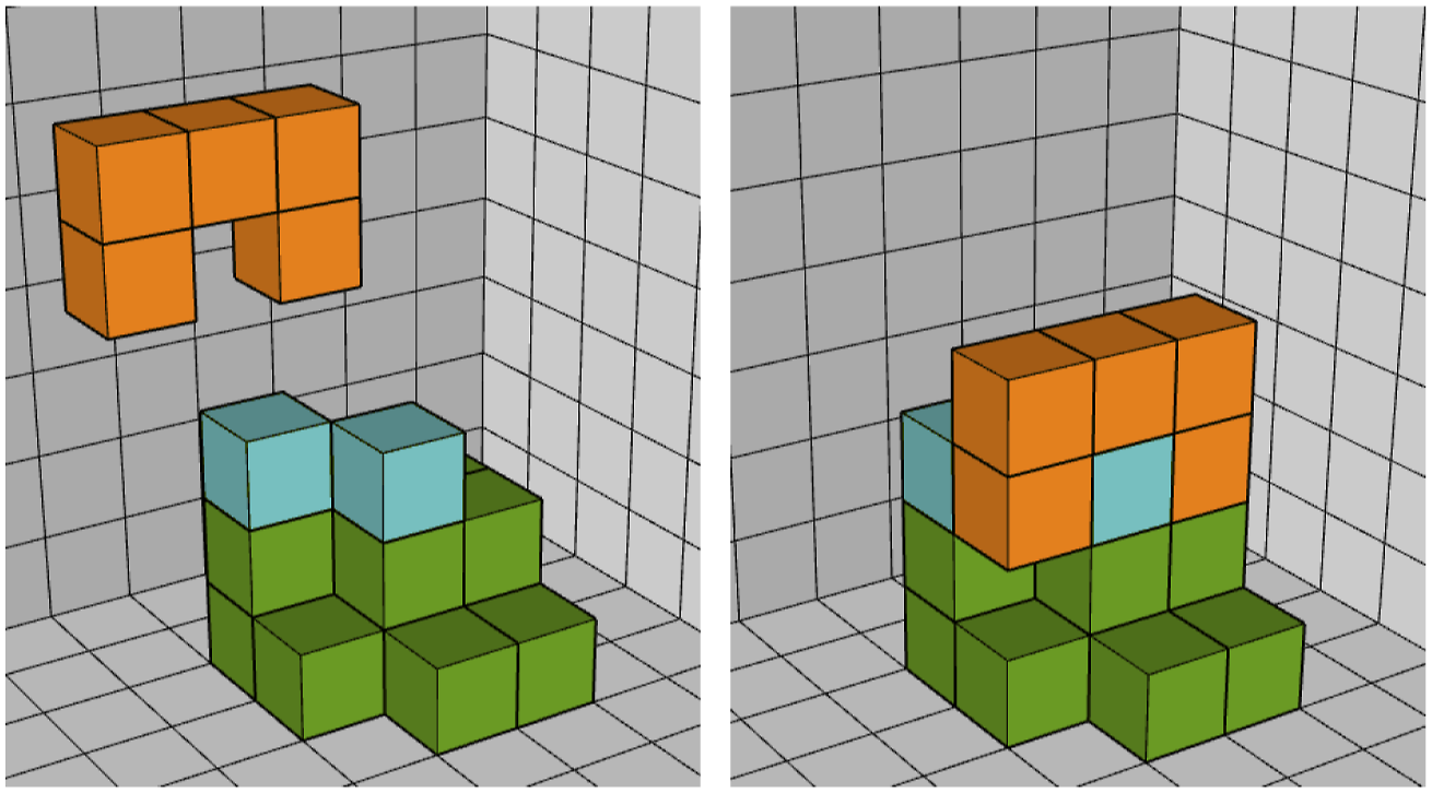

The networks are trained on a fixed set of randomly generated objects placed in random positions on a table surface, and evaluated on a new set of previously unseen objects. In the 2D case, the training set comprises 80 objects, with 125 combinations of object position and initial gripper pose. In the 3D case, the training set is composed of 6000 object shapes, with five distinct positions for the obstacle and the gripper starting pose. Evaluation results are based on 1250 trials composed of 50 environments, five trajectories and five repetitions.

6. Results and discussion

Our results demonstrate that LCI-Net, despite representing only a relatively small change in the network architectures of VIN and QMDP-Net, is able to deliver significant increases in performance and efficiency in both fully and partially observable domains.

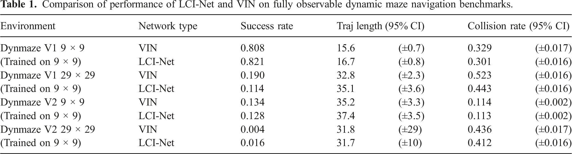
6.1. Fully observable domains

Table 1 presents a comparison of the success rate, average number of steps, and collision rate of executing the policies generated by LCI-Net and VIN on 2D navigation tasks, while Table 2 compares the same performance metrics when these trained models are evaluated on previously seen large scale realistic environments.

Table 1.

Comparison of performance of LCI-Net and VIN on fully observable dynamic maze navigation benchmarks.

Environment	Network type	Success rate	Traj length (95% CI)		Collision rate (95% CI)
Dynmaze V1 9 × 9	VIN	0.808	15.6	(±0.7)	0.329	(±0.017)
(Trained on 9 × 9)	LCI-Net	0.821	16.7	(±0.8)	0.301	(±0.016)
Dynmaze V1 29 × 29	VIN	0.190	32.8	(±2.3)	0.523	(±0.016)
(Trained on 9 × 9)	LCI-Net	0.114	35.1	(±3.6)	0.443	(±0.016)
Dynmaze V2 9 × 9	VIN	0.134	35.2	(±3.3)	0.114	(±0.002)
(Trained on 9 × 9)	LCI-Net	0.128	37.4	(±3.5)	0.113	(±0.002)
Dynmaze V2 29 × 29	VIN	0.004	31.8	(±29)	0.436	(±0.017)
(Trained on 9 × 9)	LCI-Net	0.016	31.7	(±10)	0.412	(±0.016)

Table 2.

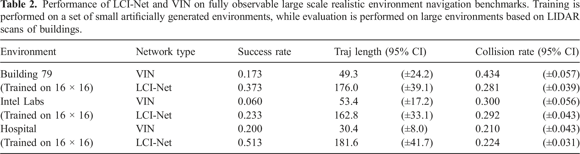
Performance of LCI-Net and VIN on fully observable large scale realistic environment navigation benchmarks. Training is performed on a set of small artificially generated environments, while evaluation is performed on large environments based on LIDAR scans of buildings.

Environment	Network type	Success rate	Traj length (95% CI)		Collision rate (95% CI)
Building 79	VIN	0.173	49.3	(±24.2)	0.434	(±0.057)
(Trained on 16 × 16)	LCI-Net	0.373	176.0	(±39.1)	0.281	(±0.039)
Intel Labs	VIN	0.060	53.4	(±17.2)	0.300	(±0.056)
(Trained on 16 × 16)	LCI-Net	0.233	162.8	(±33.1)	0.292	(±0.043)
Hospital	VIN	0.200	30.4	(±8.0)	0.210	(±0.043)
(Trained on 16 × 16)	LCI-Net	0.513	181.6	(±41.7)	0.224	(±0.031)

Several important conclusions can be taken from these results. By introducing LCI-Net to the VIN architecture, higher success rates and lower collision rates are delivered in almost all tests, with shorter average trajectory lengths in many cases even when success rate is substantially higher for LCI-Net. These results indicate that a better policy can be generated simply by replacing the forward propagation module of VIN with LCI-Net.

Additionally, the disparity in performance between the architectures increases as the size of the evaluation domain grows larger than the training domain, with LCI-Net producing significantly higher success rates in the 28 × 28, 40 × 40 and realistic environment cases. This shows that introducing LCI-Net substantially improves the generalisation capability of VIN, enabling agents to operate in large environments while only requiring trajectories produced from small artificial domains for training.

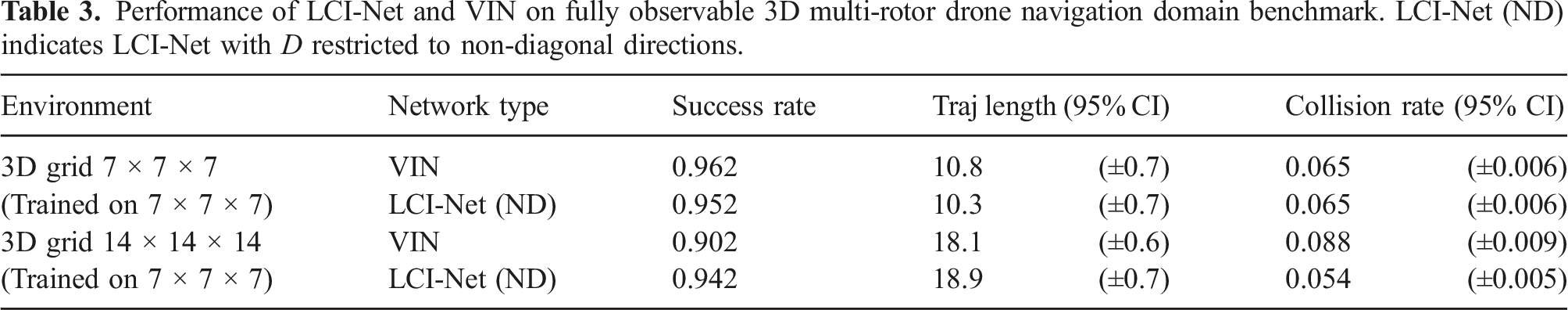
Table 3 shows comparison results for fully observable 3D multi-rotor drone navigation task. Here, performance is similar between the two networks when evaluated on the same domain size as used for training, but LCI-Net shows greater advantage in both success rate and collision rate as the evaluation environment size is increased beyond the size of the training environment.

Table 3.

Performance of LCI-Net and VIN on fully observable 3D multi-rotor drone navigation domain benchmark. LCI-Net (ND) indicates LCI-Net with D restricted to non-diagonal directions.

Environment	Network type	Success rate	Traj length (95% CI)		Collision rate (95% CI)
3D grid 7 × 7 × 7	VIN	0.962	10.8	(±0.7)	0.065	(±0.006)
(Trained on 7 × 7 × 7)	LCI-Net (ND)	0.952	10.3	(±0.7)	0.065	(±0.006)
3D grid 14 × 14 × 14	VIN	0.902	18.1	(±0.6)	0.088	(±0.009)
(Trained on 7 × 7 × 7)	LCI-Net (ND)	0.942	18.9	(±0.7)	0.054	(±0.005)

6.2. Partially observable domains

Moving to partially observable domains, where LCI-Net is able to enhance both value and state estimation, further highlights the substantial increase in performance which can be enabled by integrating LCI-Net.

Table 4 presents comparisons on the success rate, average number of steps, and collision rate of executing the policies generated by LCI-Net and by QMDP-Net for the partially observable dynamic maze environment tasks. Table 4 shows the performance of LCI-Net on the same task where D is restricted to non-diagonal shift directions.

Table 4.

Performance of LCI-Net and QMDP-Net on the partially observable 2D dynamic maze domain. LCI-Net represents our network incorporating LCI-Net with all possible shift directions included, LCI-Net (ND) represents our network with only non-diagonal shift directions included.

Environment	Network type	Success rate	Traj (95% CI)		Col rate (95% CI)
Dynmaze V1 9 × 9	QMDP-Net	0.887	23.7	(±1.1)	0.226	(±0.009)
(Trained on 9 × 9)	LCI-Net	0.942	20.2	(±0.8)	0.195	(±0.008)
	LCI-Net (ND)	0.985	18.6	(±0.7)	0.157	(±0.007)
Dynmaze V1 29 × 29	QMDP-Net	0.031	23.7	(±1.1)	0.226	(±0.009)
(Trained on 9 × 9)	LCI-Net	0.302	20.2	(±0.8)	0.195	(±0.008)
	LCI-Net (ND)	0.743	18.6	(±0.7)	0.157	(±0.007)
Dynmaze V2 9 × 9	QMDP-Net	0.808	24.1	(±1.2)	0.213	(±0.008)
(Trained on 9 × 9)	LCI-Net	0.978	18.7	(±0.8)	0.123	(±0.005)
	LCI-Net (ND)	0.971	18.6	(±0.8)	0.135	(±0.006)
Dynmaze V2 29 × 29	QMDP-Net	0.091	71.8	(±0.7)	0.412	(±0.009)
(Trained on 9 × 9)	LCI-Net	0.590	59.7	(±2.4)	0.228	(±0.011)
	LCI-Net (ND)	0.604	60.7	(±2.3)	0.148	(±0.005)

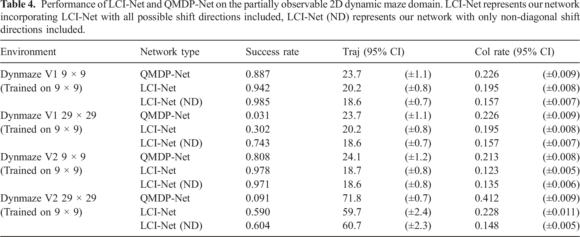
A number of key conclusions can be drawn from these results. First, by incorporating LCI-Net into QMDP-Net, we are able to produce consistently higher success rates and lower collision rates, compared to the original QMDP-Net. In the cases where success rates are closest between the networks, LCI-Net produces average trajectory lengths which are near or below those produced by QMDP-net. This applies both when D includes all possible shifts and when D is selected to contain non-diagonal shifts only, with the non-diagonal variant delivering comparable or better performance than the version which uses all possible shift directions.

Secondly, as also observed in the fully observable domains, the size of the disparity between the performance of the architectures becomes dramatic when the learned models are generalised to larger environments. In Dynamic Maze V1, the success rate of QMDP-Net drops by more than 95% when environment size is increased to 29 × 29, while the ND variant of LCI-Net has its success rate reduced by less than 25%. The V2 maze variant gives similar results - the QMDP-Net success rate drops by almost 90%, while the ND version of LCI-Net drops by less than 40%.

The results indicate that the introduction of LCI-Net greatly improves the generalisation capability of QMDP-Net, allowing effective policies to be found in large environments while requiring only expert trajectories on small environments for training. This result is likely enabled by the greater domain knowledge able to be encoded via the structure of the LCI-Net forward propagation. This represents a significant step towards making end-to-end learning for planning practical for real world applications.

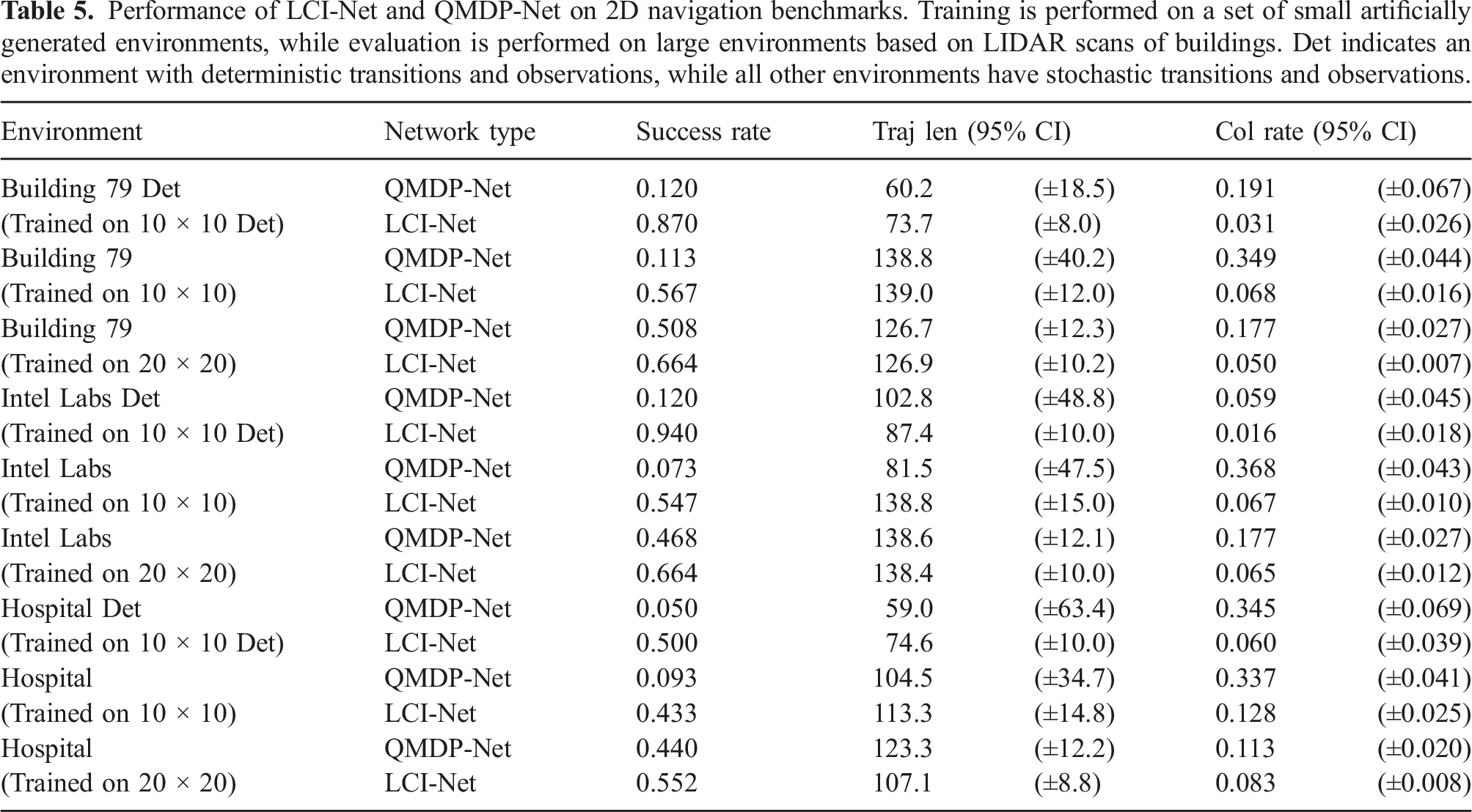
Table 5 shows a comparison of the performance of policies produced by LCI-Net and by QMDP-Net for the partially observable 2D navigation tasks. The trends from the dynamic maze tasks continue. LCI-Net consistently produces a higher overall level of policy performance, with the distinction between the networks most pronounced when training is performed on the smaller 10×10 environments. The policy produced by QMDP-Net from the 10×10 returned a success rate of below 15% in each of the trialed environments, while the policy produced by LCI-Net achieves success rates above 50% for all but one of the environments, and above 80% for two environments.

Table 5.

Performance of LCI-Net and QMDP-Net on 2D navigation benchmarks. Training is performed on a set of small artificially generated environments, while evaluation is performed on large environments based on LIDAR scans of buildings. Det indicates an environment with deterministic transitions and observations, while all other environments have stochastic transitions and observations.

Environment	Network type	Success rate	Traj len (95% CI)		Col rate (95% CI)
Building 79 Det	QMDP-Net	0.120	60.2	(±18.5)	0.191	(±0.067)
(Trained on 10 × 10 Det)	LCI-Net	0.870	73.7	(±8.0)	0.031	(±0.026)
Building 79	QMDP-Net	0.113	138.8	(±40.2)	0.349	(±0.044)
(Trained on 10 × 10)	LCI-Net	0.567	139.0	(±12.0)	0.068	(±0.016)
Building 79	QMDP-Net	0.508	126.7	(±12.3)	0.177	(±0.027)
(Trained on 20 × 20)	LCI-Net	0.664	126.9	(±10.2)	0.050	(±0.007)
Intel Labs Det	QMDP-Net	0.120	102.8	(±48.8)	0.059	(±0.045)
(Trained on 10 × 10 Det)	LCI-Net	0.940	87.4	(±10.0)	0.016	(±0.018)
Intel Labs	QMDP-Net	0.073	81.5	(±47.5)	0.368	(±0.043)
(Trained on 10 × 10)	LCI-Net	0.547	138.8	(±15.0)	0.067	(±0.010)
Intel Labs	QMDP-Net	0.468	138.6	(±12.1)	0.177	(±0.027)
(Trained on 20 × 20)	LCI-Net	0.664	138.4	(±10.0)	0.065	(±0.012)
Hospital Det	QMDP-Net	0.050	59.0	(±63.4)	0.345	(±0.069)
(Trained on 10 × 10 Det)	LCI-Net	0.500	74.6	(±10.0)	0.060	(±0.039)
Hospital	QMDP-Net	0.093	104.5	(±34.7)	0.337	(±0.041)
(Trained on 10 × 10)	LCI-Net	0.433	113.3	(±14.8)	0.128	(±0.025)
Hospital	QMDP-Net	0.440	123.3	(±12.2)	0.113	(±0.020)
(Trained on 20 × 20)	LCI-Net	0.552	107.1	(±8.8)	0.083	(±0.008)

Table 6 shows results for the partially observable 3D multi-rotor drone navigation task. Both network architectures are able to produce high rates of success and low rates of collision when evaluated on environments of the same size as used in training. Increasing the scale and complexity of the evaluation environment again shows an advantage in performance produced by LCI-Net.

Table 6.

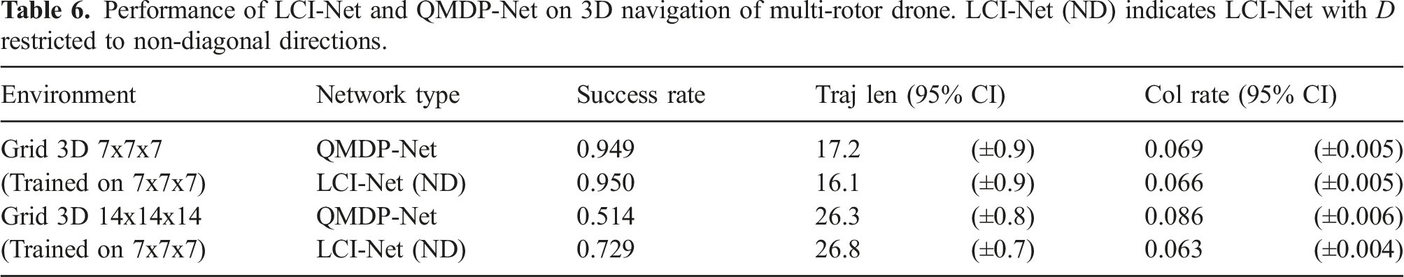
Performance of LCI-Net and QMDP-Net on 3D navigation of multi-rotor drone. LCI-Net (ND) indicates LCI-Net with D restricted to non-diagonal directions.

Environment	Network type	Success rate	Traj len (95% CI)		Col rate (95% CI)
Grid 3D 7x7x7	QMDP-Net	0.949	17.2	(±0.9)	0.069	(±0.005)
(Trained on 7x7x7)	LCI-Net (ND)	0.950	16.1	(±0.9)	0.066	(±0.005)
Grid 3D 14x14x14	QMDP-Net	0.514	26.3	(±0.8)	0.086	(±0.006)
(Trained on 7x7x7)	LCI-Net (ND)	0.729	26.8	(±0.7)	0.063	(±0.004)

Table 7 presents results for the partially observable object grasping tasks. Here, LCI-Net continues to produce higher success rates. Both networks are able to produce effective policies for 3D grasping on environments with the same dimensions as the training set, though generalising to larger environments is challenging for both architectures, with LCI-Net giving a small advantage in success rate.

Table 7.

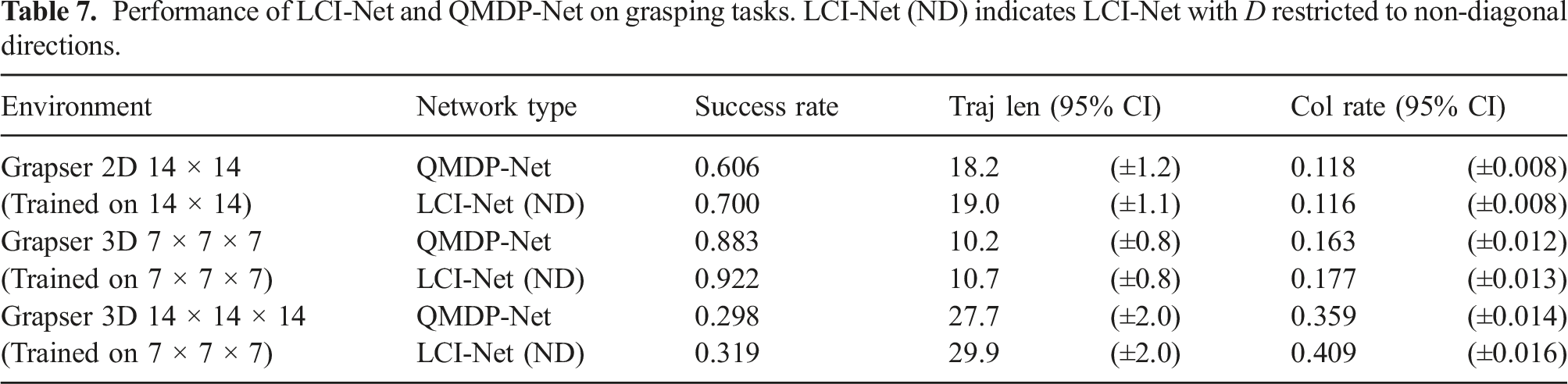
Performance of LCI-Net and QMDP-Net on grasping tasks. LCI-Net (ND) indicates LCI-Net with D restricted to non-diagonal directions.

Environment	Network type	Success rate	Traj len (95% CI)		Col rate (95% CI)
Grapser 2D 14 × 14	QMDP-Net	0.606	18.2	(±1.2)	0.118	(±0.008)
(Trained on 14 × 14)	LCI-Net (ND)	0.700	19.0	(±1.1)	0.116	(±0.008)
Grapser 3D 7 × 7 × 7	QMDP-Net	0.883	10.2	(±0.8)	0.163	(±0.012)
(Trained on 7 × 7 × 7)	LCI-Net (ND)	0.922	10.7	(±0.8)	0.177	(±0.013)
Grapser 3D 14 × 14 × 14	QMDP-Net	0.298	27.7	(±2.0)	0.359	(±0.014)
(Trained on 7 × 7 × 7)	LCI-Net (ND)	0.319	29.9	(±2.0)	0.409	(±0.016)

Table 8 provides a comparison of the time and memory required for training for each environment between LCI-Net and QMDP-Net. The more expressive transition operator incorporated in LCI-Net introduces only a small amount of extra complexity. The additional time required per epoch of training is small in most cases, and is often compensated for by a decrease in the number of epochs of training required to reach convergence.

Table 8.

Comparison of time and resources required for training in each environment between our network with LCI-Net and QMDP-Net. LCI-Net represents our network incorporating LCI-Net with all possible shift directions included, LCI-Net (ND) represents our network with only non-diagonal shift directions included. Time per epoch is in mm:ss format, while total train time is in hh:mm:ss format. Memory usage refers to the amount of GPU memory consumed-this is the only memory used for training.

Environment	Network	# Shift	Time per	Epochs to	Total train	Memory
Environment	Type	Directions	Epoch	Converge	Time	Usage (MiB)
Grid 2D 20 × 20	QMDP-Net		3:08	612	31:57:36	2333
	LCI-Net	9	3:46	678	42:33:48	2609
	LCI-Net (ND)	5	2:44	624	28:25:36	2333
Dynmaze V1 9 × 9	QMDP-Net		0:20	997	5:32:20	785
	LCI-Net	9	0:28	996	7:44:48	789
	LCI-Net (ND)	5	0:21	828	4:49:48	789
Dynmaze V2 9 × 9	QMDP-Net		0:26	920	6:38:40	1553
	LCI-Net	9	0:31	613	5:16:43	1557
	LCI-Net (ND)	5	0:26	463	3:20:38	1557
Grid 3D 7 × 7 × 7	QMDP-Net		2:48	451	21:02:48	4893
Grid 3D 7 × 7 × 7	LCI-Net (ND)	7	2:26	609	24:41:54	4913
Grasper 2D 14 × 14	QMDP-Net		5:43	544	51:49:52	527
Grasper 2D 14 × 14	LCI-Net (ND)	5	5:57	329	32:37:33	529
Grasper 3D 7 × 7 × 7	QMDP-Net		3:33	371	21:57:03	5405
Grasper 3D 7 × 7 × 7	LCI-Net (ND)	7	3:10	304	16:02:40	5421

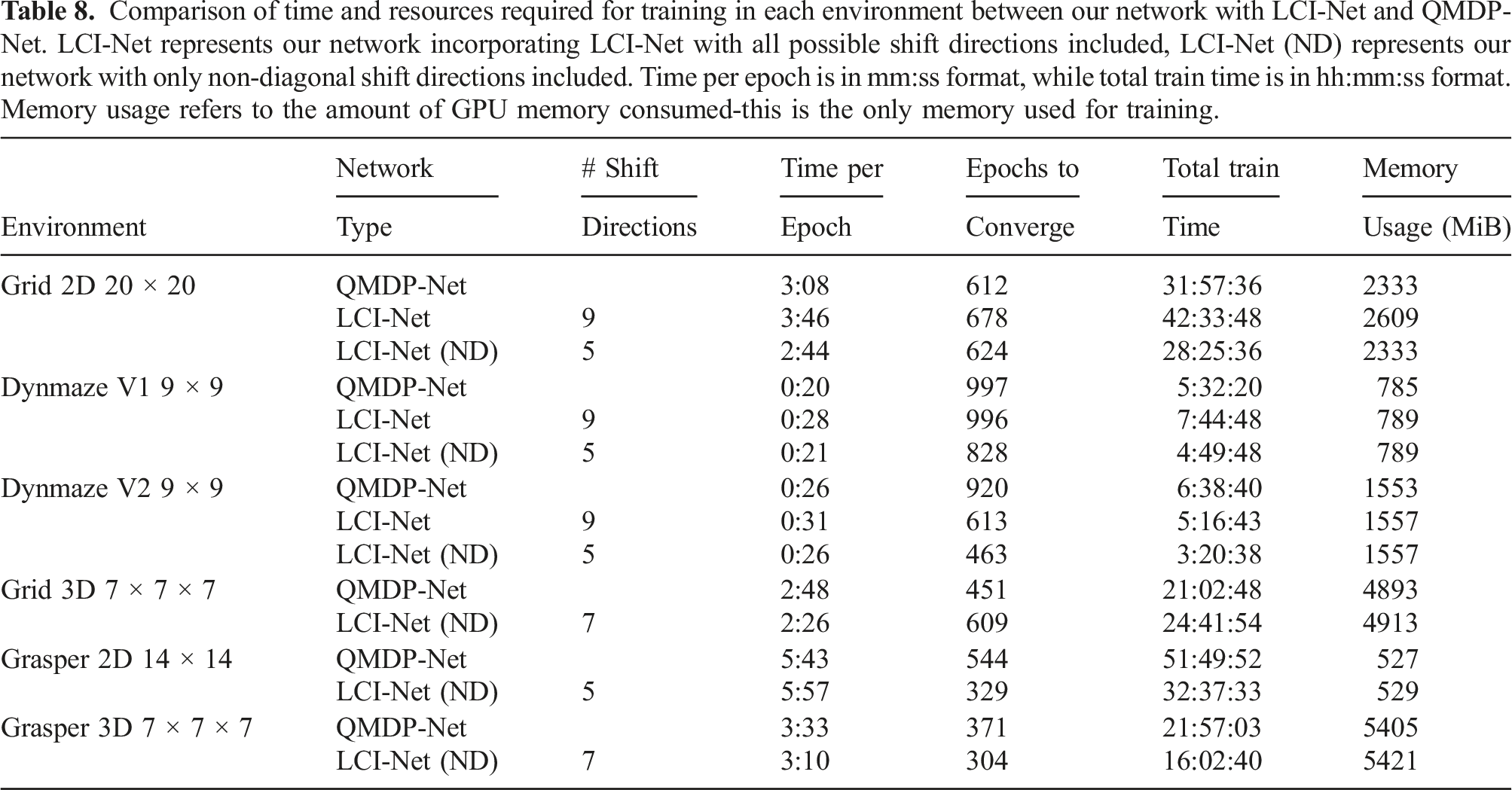
When only non-diagonal shifts are included in D, the complexity results are particularly promising. In some cases, LCI-Net with only non-diagonal shifts requires less time per epoch of training than QMDP-Net while converging in fewer epochs, resulting in a significant reduction in the total amount of time for training, while still producing policies which perform at a higher level than QMDP-Net policies.

In most cases, the additional amount of memory consumed by LCI-Net is negligible relative to total memory consumption. While scaling to larger environments results in an increase in required memory, the rate of growth in memory consumption is very close to that of QMDP-Net.

7. Summary

Many neural network architectures for solving stochastic planning with partially unknown models based on end-to-end learning have been proposed. Across these architectures, there are a number of seemingly small components that have been used repeatedly, creating a great potential benefit in improving the efficiency of these components. Improvements in these components will likely improve the overall performance, similar to how improvement in ‘primitive’ computations in motion planning improves the performance of the overall planning capability. Taking a step in this direction, this paper presents LCI-Net, a neural network module that computes one-step information propagation governed by a learned stochastic model of the system’s dynamics. It is a simple neural network module that can be plugged into various neural network architectures. Evaluating LCI-Net on VIN Tamar et al. (2017) and QMDP-Net Karkus et al. (2017) (and hence on E2E-HF Jonkowski and Brock, 2017), on 2D and 3D navigation and grasping benchmarks indicate that LCI-Net creates significant gains in performance, with generalisation capability increased by multiple folds.

Footnotes

Funding

The author(s) disclosed receipt of the following financial support for the research, authorship, and/or publication of this article: This work is supported by the ANU Futures Scheme. Nicholas Collins is supported by an Australian Government Research Training Program (RTP) scholarship provided by the University of Queensland.

ORCID iD

Nicholas Collins

References

Collins

Kurniawati

(2020) Locally-connected interrelated network: a forward propagation primitive. In: Proceedings of the Fourteenth Workshop on the Algorithmic Foundations of Robotics, Oulu, Finland, 21–23 June 2021.

François-Lavet

Bengio

Precup

, et al. (2019) Combined reinforcement learning via abstract representations. Association for the Advancement of Artificial Intelligence 33: 3582–3589.

Gupta

Davidson

Levine

, et al. (2017) Cognitive mapping and planning for visual navigation. In: IEEE Conference on Computer Vision and Pattern Recognition (CVPR), Honolulu, HI, 21–26 July 2017. DOI: 10.1109/cvpr.2017.769.

Haarnoja

Ajay

Levine

, et al. (2016) Backprop KF: learning discriminative deterministic state estimators. In: NIPS Conference, Barcelona, Spain, 5–10 December 2016.

Hausknecht

Stone

(2015) Deep recurrent Q-learning for partially observable MDPs. In: AAAI 2015 Fall Symposium, Arlington, VI, 12–14 November 2015.

Howard

Roy

(2003) The robotics data set repository (radish). Available at: http://radish.sourceforge.net/

Jonkowski

Brock

(2016) End-to-End Learnable Histogram Filters. In Workshop on Deep Learning for Action and Interaction at NIPS, Barcelona, Spain, 5-10 December 2016.

Kaelbling

Littman

Cassandra

(1998) Planning and acting in partially observable stochastic domains. Artificial Intelligence 101(1–2): 99–134.

Karkus

Hsu

Lee

(2017) QMDP-net: deep learning for planning under partial observability. In: NIPS Conference, Long Beach, CA, 4–9 December 2017.

10.

Karkus

Hsu

Lee

(2018) Particle filter networks with application to visual localization. In: CoRL Conference, Zürich, Switzerland, 29–31 October 2018.

11.

Karkus

Hsu

, et al. (2019) Differentiable algorithm networks for composable robot learning. In: Robotics: Science and Systems, Breisgau, Germany, 22–26 June 2019.

12.

Lever

Stafford

Shawe-Taylor

(2014) Learning transition dynamics in MDPs with online regression and greedy feature selection. In: Neural Information Processing Systems Conference Workshop on Autonomously Learning Robots, Montreal, Canada, 12 December 2014.

13.

Lee

Parisotto

Chaplot

, et al. (2018) Gated path planning networks. In: ICML Conference, Stockholm, Sweden, 10–15 July 2018.

14.

Littman

Cassandra

Kaelbling

(1995) Learning policies for partially observable environments: scaling up. In: International Conference on Machine Learning, Tahoe City, CA, 9–12 July 1995.

15.

Mirowski

Pascanu

Viola

, et al. (2016) Learning to navigate in complex environments. In: ICLR Conference, San Juan, Puerto Rico, 2–4 May 2016.

16.

Mnih

Kavukcuoglu

Silver

, et al. (2015) Human-level control through deep reinforcement learning. Nature 518: 529–533. DOI: 10.1038/nature14236.

(2017) Learning multimodal transition dynamics for model-based reinforcement learning. In: European Conference on Machine Learning, Skopje, Macedonia, 18–22 September 2017.

18.

Guo

Lee

, et al. (2015) Action-conditional video prediction using deep networks in atari games. In: NIPS Conference, Montreal, Canada, 7–12 December 2015, pp. 2863–2871.

19.

Singh

Lee

(2017) Value prediction network. In: NIPS Conference, , Long Beach, CA, 4–9 December 2017, pp. 6118–6128.

(2017) Pathe Integral Networks: Ennd-To-End Differentiable Optimal Control. arXiv preprint arXiv:1706.09597.

21.

Olah

(2019) Neural networks, types, and functional programming. Available at: http://colah.github.io/posts/2015-09-NN-Types-FP/

22.

Puterman

(2014) Markov Decision Processes: Discrete Stochastic Dynamic Programming. Hoboken, NJ: John Wiley & Sons.

23.

Qureshi

Simeonov

Bency

, et al. (2019) Motion planning networks. In: 2019 International Conference on Robotics and Automation (ICRA), Montreal, Canada, 20–24 May 2019, pp. 2118–2124. IEEE.

24.

Shankar

Dwivedy

Guha

(2016) Reinforcement learning via recurrent convolutional neural networks. In: ICPR Conference, Cancún, Mexico, 4–8 December 2016, pp. 2592–2597. DOI: 10.1109/ICPR.2016.7900026.

25.

Sondik

(1971) The Optimal Control of Partially Observable Markov processes. PhD Thesis, Stanford University: Stanford, CA.

26.

Sun

Yin

Huang

(2021) Temple: Learning template of transitions for sample efficient multi-task rl. In: AAAI Conference on Artificial Intelligence, Vancouver, Canada, 2–9 February 2021.

27.

Tamar

Thomas

, et al. (2017) Value iteration networks. In: IJCAI Conference, Melbourne, Australia, 19–25 August 2017.

28.

van der Pol

Worrall

van Hoof

, et al. (2020) Mdp homomorphic networks: group symmetries in reinforcement learning. Advances in Neural Information Processing Systems 33; 2146–2154.

29.

Wahlström

Schön

Deisenroth

(2015) Learning deep dynamical models from image pixels. In: The 17th IFAC Symposium on System Identification (SYSID), Beijing, China, 19–21 October 2015.