Linear-time quasi-static stability detection for modular self-reconfigurable robots

Abstract

We address the problem of detecting potential instability in the planned motion of modular self-reconfigurable robots. Previous research primarily focused on determining the system’s unique physical state but overlooked the mutual compensation effects of connection constraints. We introduce a linear-time quasi-static stability detection method for modular self-reconfigurable robots. The internal connections, non-connected contacts, and environmental contacts are considered, and the problem is modeled as a second-order cone program problem, whose solving time linearly increases with the number of modules. We aim to determine the critical stable state of the system and that is achieved by finding the required minimum characteristic connection strength. By analyzing the critical stable state, we can assess the system’s stability and identify potential broken connection points. Furthermore, the internal stability margin is defined to evaluate the configuration’s stability level. The suspension and object manipulation configurations are first demonstrated in simulation to analyze the effectiveness of the proposed algorithm. Subsequently, a series of physical experiments based on FreeSN were carried out. The calculated stable motion ranges of manipulator configurations are highly consistent with the actual sampling boundaries. Moreover, the proposed algorithm successfully predicts stability and identifies broken connections in diverse configurations, encompassing quadruped and closed-chain configurations on both even and uneven terrains. The load experiment further demonstrates that the impacts from unmodeled factors and input errors under normal conditions can be on a small scale. By combining the proposed detection method and stability margin, we open the door to realizing real-time motion planning on modular self-reconfigurable robots.

Keywords

Modular robot self-reconfigurable force optimization second-order cone program (SOCP)

1. Introduction

The modular self-reconfigurable robot (MSRR) system (Dokuyucu and Özmen, 2023; Seo et al., 2019; Yim et al., 2007; Alberto et al., 2017) is a type of swarm robot system composed of many identical robot modules that need to be physically connected. These modules can realize self-reconfiguration by attaching and detaching thereby altering the connection topology, promising to execute challenging tasks in unknown and unstructured environments. Many versions of reconfigurable robots, as surveyed in Liang et al. (2024), have been developed. These robots can be divided into six categories, lattice type, chain type, hybrid type, mobile structure, truss structure, and freeform. These systems have exhibited a wide variety of locomotion and manipulation, including legged walking (Hamlin and Sanderson, 1996), snake gaits (Jing et al., 2018), rolling (Sastra et al., 2009); (Shen et al., 2006), manipulation of objects (Zhao and Lam, 2022; Tu et al., 2022), climbing (Liang et al., 2020), self-reconfiguration between dozens of shapes (Butler and Rus, 2003; Suh et al., 2002), and others (Zong et al., 2023).

The diversity and flexibility of MSRR stem from its creative hardware design, namely the connector and driving mode between modules. Once the connection relationship is established, the relative motion between modules through the driver can be seen as the joint motion process. The change of connection topology can be realized by the reconfiguration process, which typically consists of three steps: (1) releasing some intermodular connections; (2) shifting modules by joint motion or independent motion; (3) creating new connections at the new location. The MSRR system must consider geometric and mechanical constraints during the motion, whether it performs the self-reconfiguration process or pure joint motion. If the MSRR system can track the planned trajectory and maintain kinematic relationships between modules to form the desired geometric shape, it meets the geometric constraints. Numerous self-reconfiguration algorithms exist to handle geometric constraints (Luo and Lam, 2023; Yao et al., 2019; Varshavskaya et al., 2008; Pan et al., 2023; Yoshida et al., 2002). However, algorithms that address mechanical constraints are relatively rare.

The connectors must provide sufficient constraints to limit the relative motion between modules to form a stable connection. However, when the load carried by the connector is too large or even exceeds the limits of the connector, geometric deformation or connection breakage will occur, which brings severe damage to the mechanism and even results in mission failure (Yim et al., 2001). We regard the unexpected connection breakage and whole-body instability as violating the mechanical constraints of MSRR. Real-time mechanical stability detection, whose invocation times are similar to obstacle avoidance algorithm and will be executed by modules using limited computation resources, is the prerequisite for performing self-reconfiguration and joint motion. We aim to find an effective modeling method for the detection of mechanical connection stability, taking into account the balance between accuracy and computational efficiency. This problem involves the following aspects: (1) how to effectively model the connector and account for its anisotropic strength; (2) how to model the whole-body stability of the system; (3) how to know the stability of internal connections given the configuration, external active forces and environmental information; (4) how to achieve a balance between model accuracy and computational cost. We limit the research scope of this paper to the quasi-static field, which means the motions are slow enough and inertial, Coriolis and centrifugal effects can be negligible.

1.1. Related work

If the stiffness of the module body significantly exceeds the stiffness of the connector, which is often the case, any configuration of MSRR can be represented as a multi-body system connected by connectors. By assessing whether the connector can provide a sufficient reaction force, one can determine the stability of the connection under quasi-static conditions. However, determining the required internal reaction force is challenging due to the presence of redundant constraints, which originate from two possible sources. One source comes from external contacts. For example, in a 2D environment, the presence of more than two environmental frictional contact points can yield infinite solutions to the equilibrium equations, resulting in an infinite number of possible internal stress distributions for MSRR. On the other hand, a module may be connected to multiple modules or form non-connected contacts, potentially leading to internal redundant constraints.

By introducing the flexible model, the reaction force can be uniquely determined (Hiller and Lipson, 2014, 2012). However, these results can be recognized as unique and credible only when the flexibility of the real system is properly reflected by the model (Wojtyra, 2017; García De Jalón and Gutiérrez-López, 2013). Paul J. White et al. (White et al., 2011) pioneered a detailed analysis of the mechanical constraints in programmable matter and MSRR, introducing a general stiffness model to characterize the strength of the connector. They utilized potential functions in Zhang and Fasse (2000) to model the wrench on the elastic connector, and the proposed non-linear model can be solved in O (n^1.4) time complexity as the number of modules n increases. Their method has been verified on CKBot (Sastra et al., 2009), Rubik’s snake, and RATChET7mm (White et al., 2011). Jakub Lengiewicz et al. proposed a distributed algorithm based on a linear-elastic finite element (FE) model to predict the unstable reconfiguration scenarios of densely MSRR systems and some numerical results are shown (Hołobut et al., 2020; Hołobut and Lengiewicz, 2017). Further, this method was applied to the Blinky Blocks and experimental results demonstrate this method can predict the unstable scenarios successfully in some cases (Piranda et al., 2021). However, to facilitate model simplicity, the prediction accuracy of this method appears to be relatively low, as demonstrated by a failure case presented by the authors. Additionally, none of the aforementioned studies accounted for the influence of friction and diverse terrains. Fully accounting for the influence of flexibility on the system will enhance the accuracy of predictions, yet it will also increment the computational complexity of the model, which is detrimental for real-time detection. Conversely, a simplified model may limit accuracy as its results may not fully capture the system’s state. Besides, the FE-based methods neglect the mutual complement effects of connection constraints. This prompts us to explore alternative approaches to achieve a more optimal balance between model accuracy and computational cost.

The amplitude of internal reaction forces is significantly influenced by external forces, including active applied forces and environmental reaction forces, necessitating concurrent consideration of whole-body balance and internal connection stability. The quasi-static whole-body balance algorithms of multi-body systems have been extensively researched and these are expected to provide valuable insights for us. Quasi-static equilibrium postures received considerable attention in the early multi-legged locomotion literature (Marhefka and Orin, 1997; McGhee and Frank, 1968; Or and Várkonyi, 2021; Or and Rimon, 2010) and humanoid robots field (Khatib et al., 2022). The support polygon principle is the leading concept to quickly check the stability of legged robots, which is also utilized to detect the whole-body stability of MSRR (Piranda et al., 2021; Luo and Lam, 2022). However, when the multi-body system is exploring the unstructured environment, this criterion fails (Bretl and Lall, 2008). For a multi-body system with multiple environmental contact points, if a set of contact forces exists that meets the equilibrium equations and friction constraints, this system is said to be weakly stable (Pang and Trinkle, 2000), which means the system may lose stability under minor external disturbances. A contact model considering the contact surface can assist us in obtaining a more precise estimation of the system state (Rimon et al., 2008; Or and Rimon, 2017). Nevertheless, this also means extra model complexity. Proving the existence of weakly stable solutions and calculating the stability margin of the system are more commonly applied methods (Grand et al., 2004; McGhee, 1967; McGhee and Frank, 1968; Ju et al., 2024; Park et al., 2019). A fast algorithm is proposed to test the static equilibrium of legged robots and deal with the contact error in Del Prete et al. (2016). Xuan Lin et al. (Lin et al., 2019) planned the contact force of legged robots and used safety factors to prevent slipping.

The quasi-static stability problem of MSRR can be regarded as a further development of these problems, with two main distinctions. Firstly, unlike traditional legged robots with only two or three internal joints for each leg, the internal connections of MSRR can be numerous and their stability must be assessed. Secondly, two types of stability margins need to be taken into account: the whole-body stability margin and the internal stability margin, which refers to the weakest connection points.

1.2. Contributions

In this paper, a linear-time quasi-static stability detection method for MSRR is proposed, which can provide stability detection of any configuration in uneven frictional terrain under known external wrenches. We consider each module as an independent entity. As long as each module can maintain stability, the entire system is stable. Each module may be subject to three types of interactions: connection, non-connected contact with neighboring modules, and environmental frictional contact. The connectors between modules are modeled to provide complete six-dimensional constraints, thus rendering the entire system passive under external wrenches. We aim not only to determine whether a system is stable, but also to calculate the internal stability margin for the stable configurations. For unstable configurations, we seek to ascertain the required minimum connection constraints to achieve this configuration. This problem is modeled as a second-order cone program (SOCP) problem, which can be easily solved by modern solver, by considering the equilibrium equations of each module, contact constraints and connector constraints. The characteristic connection strength is first defined and by modifying the weight values, the anisotropic stiffness of connectors can be reflected. We set the minimum characteristic connection strength as the main optimization objective to obtain the critical stable state of the system. This critical stable state reflects the minimum internal connection wrench required for maintaining system stability, as well as the contact state and potential broken connection points. By comparing the maximum connection wrench of the physical system, we can easily know whether the system is stable and calculate the internal stability margin. FreeSN (Tu et al., 2022) is used to verify the method we proposed. We constructed different configurations of FreeSN and confirmed the performance of the proposed model through comprehensive simulation and physical experiments, demonstrating the usability and accuracy of the method.

The main contributions contain:

1. A linear-time method for detecting the quasi-static stability of MSRR on uneven terrain is proposed. This method fully takes into account connector constraints, environmental frictional contacts, and non-connected contacts. It enables fast and reliable stability detection and identification of potential broken connection points.

2. An internal stability margin calculation model for MSRR is proposed based on the stability detection method, which serves as a reliable indicator for assessing the stability level of MSRR configurations.

3. A series of simulation and physical experiments conducted on FreeSN verified the prediction accuracy and computation efficiency of our method. These experiments further demonstrate that the proposed method effectively accounts for the geometric distribution of the system and accurately identifies potential broken connection points.

According to the knowledge of the authors, this is the first paper to propose a non-FE model for the detection of MSRR stability, while also considering the influence of uneven frictional terrains. Additionally, the internal stability margin for MSRR is also the first time to be discussed.

1.3. Structure

The remainder of this paper is organized as follows: Section 2 models the quasi-static stability constraints for MSRR, including equilibrium constraints and inequality constraints. Section 3 introduces the connector constraints and further systematically proposes the SOCP detection model and stability theorem for MSRR. The characteristic connection strength, internal stability margin and potential broken connection points are also discussed in this part. Section 4 presents the complete stability algorithm based on the aforementioned framework, detailing the algorithm’s execution flow and specifics. In Section 5, we introduce the connection characteristic of FreeSN and further derive the stability detection model for FreeSN, considering the coupling relationships in connector constraints. This section also includes simulation analysis of two configurations with numerous modules. Physical experiments and algorithm computation complexity analysis are detailed in Section 6. We conclude our work and discuss the future work in Section 7.

2. Quasi-static stability constraints for MSRR

2.1. Connector model and unstable situations

The entire MSRR system can be seen as the combination of rigid modules and connectors as shown in Figure 1(a). Typically, the module body can be abstracted as a simple geometry such as a sphere (Hołobut and Lengiewicz, 2017), a cube (Piranda et al., 2021), or others, depending on its specific geometrical features. In this paper, we discuss a general method for detecting the quasi-static stability of MSRR; therefore, the geometric features of the modules are expressed abstractly. Numerous connection methods have been explored for constructing MSRR systems, including latch, lock, hooks, electrical magnets, permanent magnets, and others (Chennareddy et al., 2017). In general, these can be divided into two categories: mechanical connections, which are more rigid, and magnetic connections. During the reconfiguration process and joint motion, each transient state of the MSRR system must be statically stable, meaning the connectors can provide all degrees of freedom constraints to limit the motion of the module.

Figure 1.

(a) The modules in an MSRR system maintain the stability through connections, non-connected contacts, and environmental contacts under known external wrenches. (b) The coordinate systems of a module i include four types: child connection coordinate tsystem ΣA, parent connection coordinate system ΣP, non-connected contact coordinate system 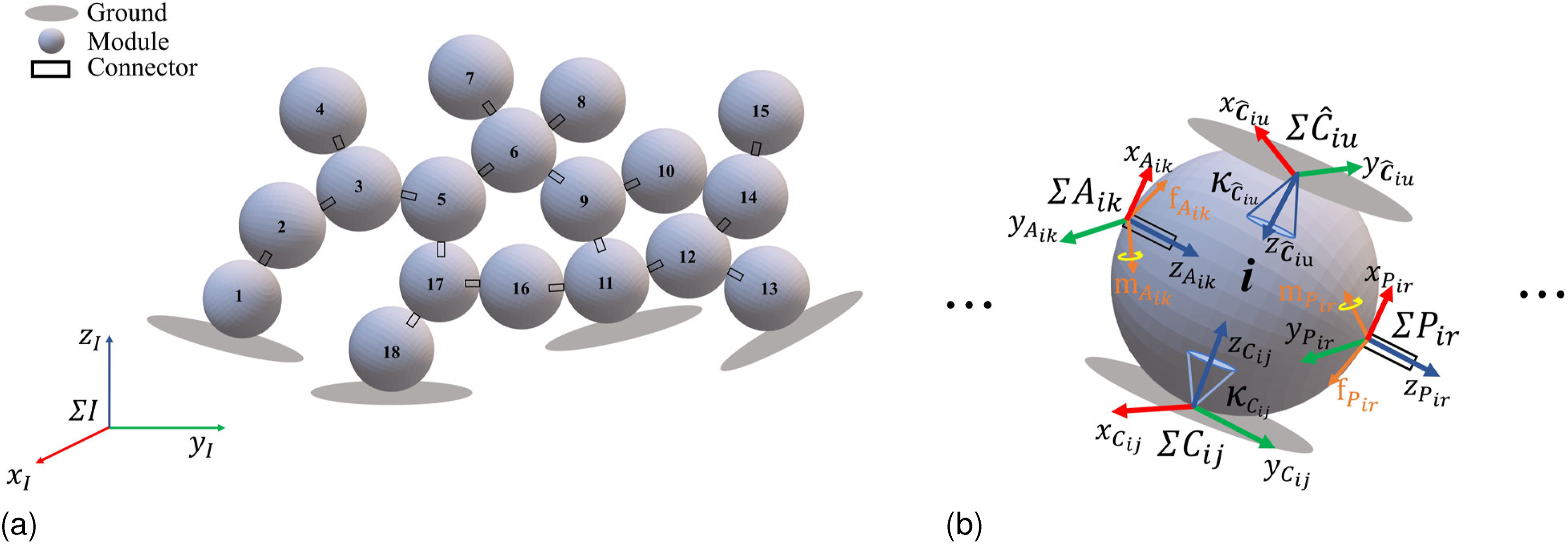$Σ \hat{C}$ , and environmental contact coordinate system ΣC. Among these, the z-axis of ΣP always points to the exterior region, while those of ΣA, $Σ \hat{C}$ , and ΣC point to the interior region of the module.

Theoretically, any type of connector can be modeled as a provider of fixed constraints. They provide constraints in all six dimensions, including displacement in the x, y, z axes and rotation around these axes. However, their capabilities in each dimension are different. We further divide the directions along the x, y, z axes into the tangential direction in the x-y plane, and the normal direction, corresponding to the z-axis. The connectors can provide force and torque in both directions to independently hinder the displacement and rotational motion of the module, corresponding to four types of unstable situations. Furthermore, considering whole-body stability, there are a total of five unstable situations.

2.2. Connection and contact

Each module is seen as an independent rigid body and can interact with the environment and other modules in three ways: connection, environmental contact, and non-connected contact. Among these, the connections are further divided into child connections and parent connections to distinguish between the two connected modules, allowing the z-axis direction of the local coordination system to be uniquely defined. The z-axis direction of the connection coordination system always points from the connection point to the geometric center of the child module. Some modules contact the external environment, and the z-axis direction of the contact coordination system also points to the interior region of the module. Additionally, a module may contact other modules without being connected, like modules 10 and 14 in Figure 1(a).

Therefore, four types of coordinate systems may simultaneously exist for one module in the MSRR system as shown in Figure 1(b): child connection, parent connection, non-connected contact and environmental contact. For the entire MSRR system to be stable, each module must be stable, and their connections and contacts must provide sufficient resultant force and torque to counteract external wrenches. The effect of external wrenches on a single module is transmitted to the surrounding modules through connections and contacts.

2.3. Equilibrium constraints

We model the stability problem based on the following assumption:

Assumption 1

The stiffness of the connector is much weaker than that of the body.

This assumption ensures that the module body will not be destroyed before instability occurs. In this paper, point contact is utilized, but the proposed method can be easily extended to surface contact (Bouyarmane et al., 2019; Nikolić et al., 2018). We first define the notations as shown in Table 1. Scalars are represented in italic lowercase letters. Vectors are denoted in lowercase bold characters, matrices in bold uppercase characters, and coordinate systems in italic uppercase characters.

Table 1.

Nomenclature.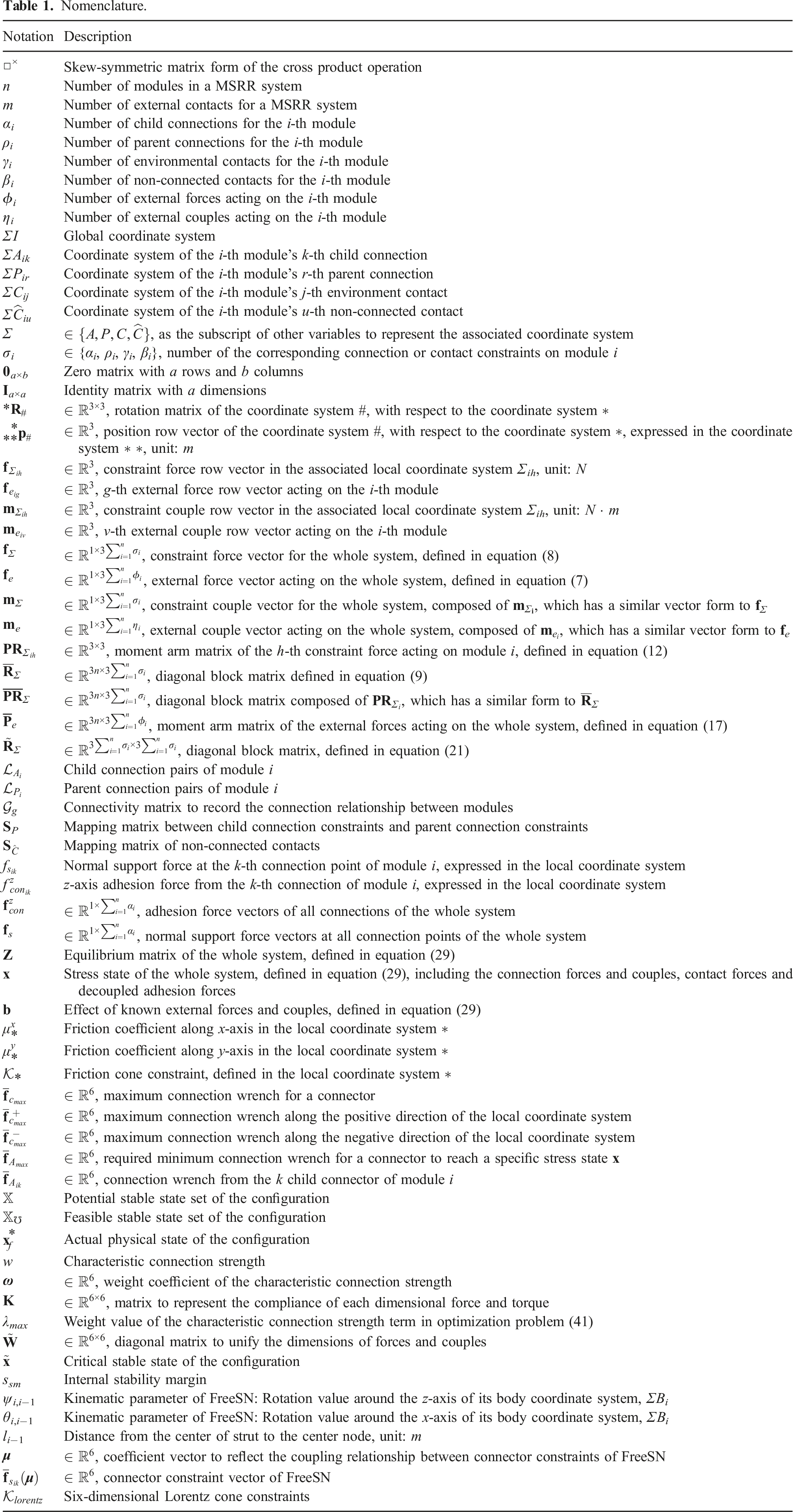

Notation	Description
□^×	Skew-symmetric matrix form of the cross product operation
n	Number of modules in a MSRR system
m	Number of external contacts for a MSRR system
α _i	Number of child connections for the i-th module
ρ _i	Number of parent connections for the i-th module
γ _i	Number of environmental contacts for the i-th module
β _i	Number of non-connected contacts for the i-th module
ϕ _i	Number of external forces acting on the i-th module
η _i	Number of external couples acting on the i-th module
ΣI	Global coordinate system
ΣA _ik	Coordinate system of the i-th module’s k-th child connection
ΣP _ir	Coordinate system of the i-th module’s r-th parent connection
ΣC _ij	Coordinate system of the i-th module’s j-th environment contact
$Σ {\hat{C}}_{i u}$	Coordinate system of the i-th module’s u-th non-connected contact
Σ	$\in {A, P, C, \hat{C}}$ , as the subscript of other variables to represent the associated coordinate system
σ _i	∈ {α_i, ρ_i, γ_i, β_i}, number of the corresponding connection or contact constraints on module i
0 _a×b	Zero matrix with a rows and b columns
I _a×a	Identity matrix with a dimensions
*R_#	$\in R^{3 \times 3}$ , rotation matrix of the coordinate system #, with respect to the coordinate system ∗
$\overset{}{*} p_{#}$	$\in R^{3}$ , position row vector of the coordinate system #, with respect to the coordinate system ∗, expressed in the coordinate system ∗ ∗, unit: m
$f_{Σ_{i h}}$	$\in R^{3}$ , constraint force row vector in the associated local coordinate system Σ_ih, unit: N
$f_{e_{i g}}$	$\in R^{3}$ , g-th external force row vector acting on the i-th module
$m_{Σ_{i h}}$	$\in R^{3}$ , constraint couple row vector in the associated local coordinate system Σ_ih, unit: N ⋅ m
$m_{e_{i v}}$	$\in R^{3}$ , v-th external couple row vector acting on the i-th module
f _Σ	$\in R^{1 \times 3 \sum_{i = 1}^{n} σ_{i}}$ , constraint force vector for the whole system, defined in equation (8)
f _e	$\in R^{1 \times 3 \sum_{i = 1}^{n} ϕ_{i}}$ , external force vector acting on the whole system, defined in equation (7)
m _Σ	$\in R^{1 \times 3 \sum_{i = 1}^{n} σ_{i}}$ , constraint couple vector for the whole system, composed of $m_{Σ_{i}}$ , which has a similar vector form to f_Σ
m _e	$\in R^{1 \times 3 \sum_{i = 1}^{n} η_{i}}$ , external couple vector acting on the whole system, composed of $m_{e_{i}}$ , which has a similar vector form to f_e
${P R}_{Σ_{i h}}$	$\in R^{3 \times 3}$ , moment arm matrix of the h-th constraint force acting on module i, defined in equation (12)
${\bar{R}}_{Σ}$	$\in R^{3 n \times 3 \sum_{i = 1}^{n} σ_{i}}$ , diagonal block matrix defined in equation (9)
${\bar{P R}}_{Σ}$	$\in R^{3 n \times 3 \sum_{i = 1}^{n} σ_{i}}$ , diagonal block matrix composed of ${P R}_{Σ_{i}}$ , which has a similar form to ${\bar{R}}_{Σ}$
${\bar{P}}_{e}$	$\in R^{3 n \times 3 \sum_{i = 1}^{n} ϕ_{i}}$ , moment arm matrix of the external forces acting on the whole system, defined in equation (17)
${\tilde{R}}_{Σ}$	$\in ℝ^{3 \sum_{i = 1}^{n} σ_{i} \times 3 \sum_{i = 1}^{n} σ_{i}}$ , diagonal block matrix, defined in equation (21)
$L_{A_{i}}$	Child connection pairs of module i
$L_{P_{i}}$	Parent connection pairs of module i
$G_{g}$	Connectivity matrix to record the connection relationship between modules
S _P	Mapping matrix between child connection constraints and parent connection constraints
$S_{\hat{C}}$	Mapping matrix of non-connected contacts
$f_{s_{i k}}$	Normal support force at the k-th connection point of module i, expressed in the local coordinate system
$f_{c o n_{i k}}^{z}$	z-axis adhesion force from the k-th connection of module i, expressed in the local coordinate system
$f_{con}^{z}$	$\in R^{1 \times \sum_{i = 1}^{n} α_{i}}$ , adhesion force vectors of all connections of the whole system
f _s	$\in R^{1 \times \sum_{i = 1}^{n} α_{i}}$ , normal support force vectors at all connection points of the whole system
Z	Equilibrium matrix of the whole system, defined in equation (29)
x	Stress state of the whole system, defined in equation (29), including the connection forces and couples, contact forces and decoupled adhesion forces
b	Effect of known external forces and couples, defined in equation (29)
$μ_{*}^{x}$	Friction coefficient along x-axis in the local coordinate system ∗
$μ_{*}^{y}$	Friction coefficient along y-axis in the local coordinate system ∗
$K_{*}$	Friction cone constraint, defined in the local coordinate system ∗
${\bar{f}}_{c_{\max}}$	$\in R^{6}$ , maximum connection wrench for a connector
${\bar{f}}_{c_{\max}}^{+}$	$\in R^{6}$ , maximum connection wrench along the positive direction of the local coordinate system
${\bar{f}}_{c_{\max}}^{-}$	$\in R^{6}$ , maximum connection wrench along the negative direction of the local coordinate system
${\bar{f}}_{A_{\max}}$	$\in R^{6}$ , required minimum connection wrench for a connector to reach a specific stress state x
${\bar{f}}_{A_{i k}}$	$\in R^{6}$ , connection wrench from the k child connector of module i
$X$	Potential stable state set of the configuration
$X_{℧}$	Feasible stable state set of the configuration
$x_{f}^{*}$	Actual physical state of the configuration
w	Characteristic connection strength
ω	$\in R^{6}$ , weight coefficient of the characteristic connection strength
K	$\in R^{6 \times 6}$ , matrix to represent the compliance of each dimensional force and torque
λ _max	Weight value of the characteristic connection strength term in optimization problem (41)
$\tilde{W}$	$\in R^{6 \times 6}$ , diagonal matrix to unify the dimensions of forces and couples
$\tilde{x}$	Critical stable state of the configuration
s _sm	Internal stability margin
ψ _i,i−1	Kinematic parameter of FreeSN: Rotation value around the z-axis of its body coordinate system, ΣB_i
θ _i,i−1	Kinematic parameter of FreeSN: Rotation value around the x-axis of its body coordinate system, ΣB_i
l _i−1	Distance from the center of strut to the center node, unit: m
μ	$\in R^{6}$ , coefficient vector to reflect the coupling relationship between connector constraints of FreeSN
${\bar{f}}_{s_{i k}} (μ)$	$\in R^{6}$ , connector constraint vector of FreeSN
$K_{lorentz}$	Six-dimensional Lorentz cone constraints

As shown in Figure 1(b), ΣA_ik represents the coordinate system of the i-th module’s k-th child connection, and ΣP_ir represents the coordinate system of the i-th module’s r-th parent connection, where k ∈ [1, α_i] and r ∈ [1, ρ_i], respectively. Similarly, ΣC_ij denotes the coordinate system of the i-th module’s j-th environmental frictional contact, and $Σ {\hat{C}}_{i u}$ denotes the coordinate system of the i-th module’s u-th non-connected contact, where j ∈ [1, γ_i] and u ∈ [1, β_i], respectively. α_i is the number of child connections for the i-th module. Similarly, ρ_i, γ_i and β_i denote the number of parent connections, environmental contacts, and non-connected contacts, respectively. We use $Σ \in {A, P, C, \hat{C}}$ as the subscript for other variables to represent the associated coordinate systems, where A, P, C, and $\hat{C}$ correspond to the child, parent, environmental contact, and non-connected contact coordinate systems, respectively. The right subscript of Σ, such as Σ_ih, represents the corresponding i-th module’s h-th constraint coordinate system. σ_i ∈ {α_i, ρ_i, γ_i, β_i} represents the maximum number of the corresponding constraint type on module i, with h ∈ [1, σ_i]. $f_{Σ_{i h}}$ and $m_{Σ_{i h}}$ represent the constraint force and couple, respectively, in the local coordinate system Σ_ih. In connection coordinate systems, both the constraint force and couple exist, while only the constraint force exists in contact coordinate systems. The z-axis direction of the parent connection coordinate systems always points to the exterior region of the module, whereas that of the other coordinate systems points to the interior region.

2.3.1. Force equilibrium

Based on the above definitions, we can write down the force equilibrium condition for module i in the global coordinate system ΣI,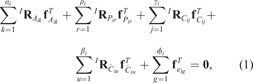

\begin{matrix} \sum_{k = 1}^{α_{i}} {}^{I}R_{A_{i k}} f_{A_{i k}}^{T} + \sum_{r = 1}^{ρ_{i}} {}^{I}R_{P_{i r}} f_{P_{i r}}^{T} + \sum_{j = 1}^{γ_{i}} {}^{I}R_{C_{i j}} f_{C_{i j}}^{T} + \\ \sum_{u = 1}^{β_{i}} {}^{I}R_{{\hat{C}}_{i u}} f_{{\hat{C}}_{i u}}^{T} + \sum_{g = 1}^{ϕ_{i}} f_{e_{i g}}^{T} = 0 \end{matrix},

(1)

where

{}^{I}R_{Σ_{i h}} \in R^{3 \times 3}

represents the rotation matrix that transforms from the local coordinate system, denoted by the right subscript Σ_ih, to the global coordinate system.

f_{e_{i g}}

is the g-th external force applied to module i. The action of gravity is also considered one type of external force. Equation (1) can be written in matrix form,

\begin{matrix} {\underset{̲}{R}}_{A_{i}} f_{A_{i}}^{T} + {\underset{̲}{R}}_{P_{i}} f_{P_{i}}^{T} + {\underset{̲}{R}}_{C_{i}} f_{C_{i}}^{T} + {\underset{̲}{R}}_{{\hat{C}}_{i}} f_{{\hat{C}}_{i}}^{T} + I_{e f_{i}} f_{e_{i}}^{T} = 0, \end{matrix}

(2)

where

{\underset{̲}{R}}_{Σ_{i}} = [{}^{I}R_{Σ_{i 1}}, {}^{I}R_{Σ_{i 2}}, \dots, {}^{I}R_{Σ_{i σ_{i}}}] \in R^{3 \times 3 σ_{i}},

(3)

f_{Σ_{i}} = [f_{Σ_{i 1}}, f_{Σ_{i 2}}, \dots, f_{Σ_{i σ_{i}}}] \in R^{1 \times 3 σ_{i}},

(4)

f_{e_{i}} = [f_{e_{i 1}}, f_{e_{i 2}}, \dots, f_{e_{i ϕ_{i}}}] \in R^{1 \times 3 ϕ_{i}},

(5)

and

I_{e f_{i}} = [I_{3 \times 3}, I_{3 \times 3}, \dots, I_{3 \times 3}] \in R^{3 \times 3 ϕ_{i}}

. Each module i ∈ [1, n] meets equation (2). The system’s force equilibrium equation can be written as

{\bar{R}}_{A} f_{A}^{T} + {\bar{R}}_{P} f_{P}^{T} + {\bar{R}}_{C} f_{C}^{T} + {\bar{R}}_{\hat{C}} f_{\hat{C}}^{T} + I_{e f} f_{e}^{T} = 0,

(6)

where

f_{e} = [f_{e_{1}}, f_{e_{2}}, \dots, f_{e_{n}}] \in R^{1 \times 3 \sum_{i = 1}^{n} ϕ_{i}},

(7)

f_{Σ} = [f_{Σ_{1}}, f_{Σ_{2}}, \dots, f_{Σ_{n}}] \in R^{1 \times 3 \sum_{i = 1}^{n} σ_{i}} .

(8)

{\bar{R}}_{Σ}

is the diagonal block matrix composed of

{\underset{̲}{R}}_{Σ_{i}}

{\bar{R}}_{Σ} = [\begin{matrix} {\underset{̲}{R}}_{Σ_{1}} & 0 & 0 & 0 \\ 0 & {\underset{̲}{R}}_{Σ_{2}} & 0 & 0 \\ 0 & 0 & ⋱ & 0 \\ 0 & 0 & 0 & {\underset{̲}{R}}_{Σ_{n}} \end{matrix}] \in R^{3 n \times 3 \sum_{i = 1}^{n} σ_{i}} .

(9)

Similarly,

I_{e f} = [\begin{matrix} I_{e f_{1}} & 0 & 0 & 0 \\ 0 & I_{e f_{2}} & 0 & 0 \\ 0 & 0 & ⋱ & 0 \\ 0 & 0 & 0 & I_{e f_{n}} \end{matrix}] \in R^{3 n \times 3 \sum_{i = 1}^{n} ϕ_{i}} .

(10)

2.3.2. Torque equilibrium

The torque equilibrium condition for module i in the global coordinate system ΣI is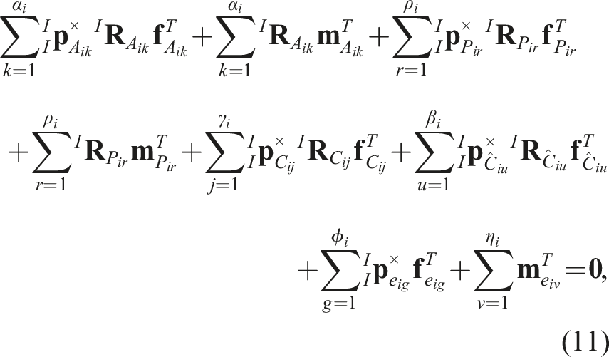

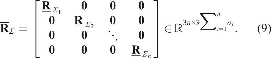
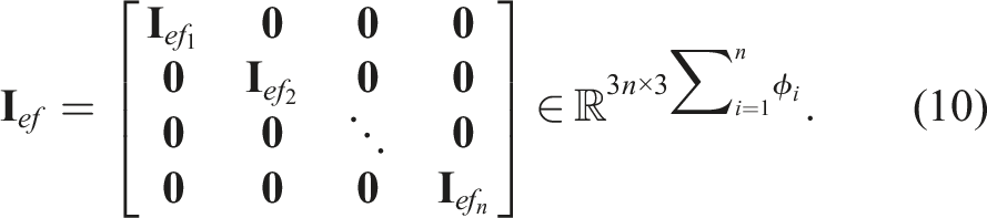
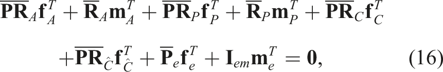
\begin{matrix} \sum_{k = 1}^{α_{i}} {}_{I}^{I}p_{A_{i k}}^{\times} {}^{I}R_{A_{i k}} f_{A_{i k}}^{T} + \sum_{k = 1}^{α_{i}} {}^{I}R_{A_{i k}} m_{A_{i k}}^{T} + & \sum_{r = 1}^{ρ_{i}} {}_{I}^{I}p_{P_{i r}}^{\times} {}^{I}R_{P_{i r}} f_{P_{i r}}^{T} \\ + \sum_{r = 1}^{ρ_{i}} {}^{I}R_{P_{i r}} m_{P_{i r}}^{T} + \sum_{j = 1}^{γ_{i}} {}_{I}^{I}p_{C_{i j}}^{\times} {}^{I}R_{C_{i j}} f_{C_{i j}}^{T} + & \sum_{u = 1}^{β_{i}} {}_{I}^{I}p_{{\hat{C}}_{i u}}^{\times} {}^{I}R_{{\hat{C}}_{i u}} f_{{\hat{C}}_{i u}}^{T} \\ + \sum_{g = 1}^{ϕ_{i}} {}_{I}^{I}p_{e_{i g}}^{\times} & f_{e_{i g}}^{T} + \sum_{v = 1}^{η_{i}} m_{e_{i v}}^{T} = 0 \end{matrix},

(11)

where

{}_{I}^{I}p_{Σ_{i h}}

is the position vector of the coordinate system Σ_ih with respect to, and expressed in, the global coordinate system. p^× is the skew-symmetric matrix form of the cross product vector p.

{}_{I}^{I}p_{e_{i g}}

is the action position vector of the g-th external force

f_{e_{i g}}

, with respect to the global coordinate system.

m_{e_{i v}}

is the v-th external couple acting on module i. We define

{P R}_{Σ_{i h}} = {}_{I}^{I}p_{Σ_{i h}}^{\times} {}^{I}R_{Σ_{i h}}, h \in [1, σ_{i}] .

(12)

Thus, we can write the above equation (11) in a more compact matrix form,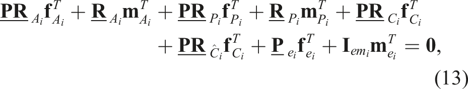

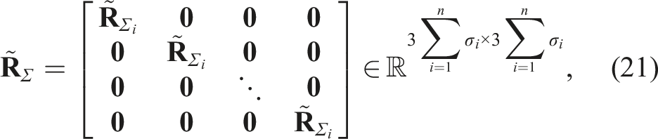
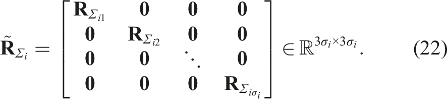
\begin{matrix} {\underset{̲}{P R}}_{A_{i}} f_{A_{i}}^{T} + {\underset{̲}{R}}_{A_{i}} m_{A_{i}}^{T} + {\underset{̲}{P R}}_{P_{i}} f_{P_{i}}^{T} + {\underset{̲}{R}}_{P_{i}} m_{P_{i}}^{T} + {\underset{̲}{P R}}_{C_{i}} f_{C_{i}}^{T} \\ + {\underset{̲}{P R}}_{{\hat{C}}_{i}} f_{C_{i}}^{T} + {\underset{̲}{P}}_{e_{i}} f_{e_{i}}^{T} + I_{e m_{i}} m_{e_{i}}^{T} = 0 \end{matrix},

(13)

where

{\underset{̲}{P R}}_{Σ_{i}}

is composed of

{P R}_{Σ_{i h}}

and have a same form to

{\underset{̲}{R}}_{Σ_{i}} \cdot

m_{Σ_{i}} \in R^{1 \times 3 σ_{i}}

and

m_{e_{i}} \in R^{1 \times 3 η_{i}}

have the same form as

f_{Σ_{i}}

and

f_{e_{i}}

, respectively. Further,

{\underset{̲}{P}}_{e_{i}} = [{}_{I}^{I}p_{e_{i 1}}^{\times}, {}_{I}^{I}p_{e_{i 2}}^{\times}, \dots, {}_{I}^{I}p_{e_{i ϕ_{i}}}^{\times}] \in R^{3 \times 3 ϕ_{i}},

(14)

and

I_{e m_{i}} = [I_{3 \times 3}, I_{3 \times 3}, \dots, I_{3 \times 3}] \in R^{3 \times 3 η_{i}} .

(15)

For each module in a MSRR system, we have the equation (13). Thus, the torque equilibrium equation of the system is

\begin{matrix} {\bar{P R}}_{A} f_{A}^{T} + {\bar{R}}_{A} m_{A}^{T} + {\bar{P R}}_{P} f_{P}^{T} + {\bar{R}}_{P} m_{P}^{T} + {\bar{P R}}_{C} f_{C}^{T} \\ + {\bar{P R}}_{\hat{C}} f_{\hat{C}}^{T} + {\bar{P}}_{e} f_{e}^{T} + I_{e m} m_{e}^{T} = 0 \end{matrix},

(16)

where

m_{Σ} \in R^{1 \times 3 \sum_{i = 1}^{n} σ_{i}}

and

m_{e} \in R^{1 \times 3 \sum_{i = 1}^{n} η_{i}}

have the same form as f_Σ and f_e.

{\bar{P R}}_{Σ} \in R^{3 n \times 3 \sum_{i = 1}^{n} σ_{i}}

and

I_{e m} \in R^{3 n \times 3 \sum_{i = 1}^{n} η_{i}}

share the diagonal block matrix form similar to that of

{\bar{R}}_{Σ}

and I_ef, and

{\bar{P}}_{e} = [\begin{matrix} {\underset{̲}{P}}_{e_{1}} & 0 & 0 & 0 \\ 0 & {\underset{̲}{P}}_{e_{2}} & 0 & 0 \\ 0 & 0 & ⋱ & 0 \\ 0 & 0 & 0 & {\underset{̲}{P}}_{e_{n}} \end{matrix}] \in R^{3 n \times 3 \sum_{i = 1}^{n} ϕ_{i}} .

(17)

2.3.3. Mutual action equilibrium of connection

If one module exerts a force or a couple on another module, then the second module exerts an equal and opposite reaction force or reaction couple on the first one. We construct S_P to describe the relationship between [f_A, m_A] and [f_P, m_P]. Because each child connection corresponds uniquely to a parent connection, we can traverse each child connection module and find the corresponding parent connection to establish an equality relationship.

As shown in Figure 1(a), each module has a unique ID, and the connection relationship between all modules in an MSRR system are recorded by a connectivity graph, which is expressed as $G_{g} \in R^{n \times n}$ . In $G_{g}$ , the i-th row represents the connections of the i-th module with other modules, where “1” indicates a child connection and “2” denotes a parent connection. The child connection pairs of module i are denoted as $L_{A_{i}}$ , and the parent connection pairs are denoted as $L_{P_{i}}$ . For example, in Figure 1(a), the connection relationship for module “5” is represented by the fifth row vector [0,0,1,0,0,2,0,0,0,0,0,0,0,0,0,0,2,0] of the matrix $G_{g}$ . Thus, $L_{A_{5}} = {< 5,3 >}$ , and $L_{P_{5}} = {< 5,6 >, < 5,17 >}$ . Based on the above definitions, we execute the following steps to create S_P.

Step 1: Let

$S_{P} = 0_{3 \sum_{i = 1}^{n} ρ_{i} \times 3 \sum_{i = 1}^{n} ρ_{i}},$

where S_P has the same row size of $f_{A}^{T}$ because

\sum_{i = 1}^{n} α_{i} = \sum_{i = 1}^{n} ρ_{i} .

(18)

Step 2: For each child connection of module i, the k-th child connection pair is represented as $< i, l_{A_{i} k} >$ within $L_{A_{i}}$ , where $l_{A_{i} k}$ is the ID number of another module. Similarly, $L_{P_{j}}$ lists all parent connection pairs for module j. Within this list, $< j, l_{P_{j} r} >$ represents the r-th parent connection pair. If the connection between module i and module j exists, the conditions $j = l_{A_{i} k}$ and $i = l_{P_{j} r}$ can always be met by traversing $L_{P_{j}}$ ; accordingly, we record the indices k, j and r.

Step 3: Letting

\begin{matrix} S_{P} (3 \sum_{h = 1}^{i - 1} α_{h} + 3 k - 2 : 3 \sum_{h = 1}^{i - 1} α_{h} + 3 k, 3 \sum_{g = 1}^{j - 1} ρ_{g} + 3 r - 2 \\ : 3 \sum_{g = 1}^{j - 1} ρ_{g} + 3 r) = I_{3 \times 3}, \end{matrix}

(19)

we establish the equality relationship between the k-th child connection of module i and the r-th parent connection of module j. The notation (a : b, c : d) specifies the selection of a submatrix from rows a to b and columns c to d.

We redo the Step 2 and Step 3 until all equality relationship are saved in S_P.

Step 4: Considering the connection constraints expressed in the local coordinate system, we can obtain the mutual action equilibrium of connection as

\begin{matrix} [\begin{matrix} {\tilde{R}}_{A} & 0 & S_{P} {\tilde{R}}_{P} & 0 \\ 0 & {\tilde{R}}_{A} & 0 & S_{P} {\tilde{R}}_{P} \end{matrix}] [\begin{matrix} f_{A}^{T} \\ m_{A}^{T} \\ f_{P}^{T} \\ m_{P}^{T} \end{matrix}] = 0 \end{matrix},

(20)

where

{\tilde{R}}_{Σ} = [\begin{matrix} {\tilde{R}}_{Σ_{i}} & 0 & 0 & 0 \\ 0 & {\tilde{R}}_{Σ_{i}} & 0 & 0 \\ 0 & 0 & ⋱ & 0 \\ 0 & 0 & 0 & {\tilde{R}}_{Σ_{i}} \end{matrix}] \in ℝ^{3 \sum_{i = 1}^{n} σ_{i} \times 3 \sum_{i = 1}^{n} σ_{i}},

(21)

{\tilde{R}}_{Σ_{i}} = [\begin{matrix} R_{Σ_{i 1}} & 0 & 0 & 0 \\ 0 & R_{Σ_{i 2}} & 0 & 0 \\ 0 & 0 & ⋱ & 0 \\ 0 & 0 & 0 & R_{Σ_{i σ_{i}}} \end{matrix}] \in ℝ^{3 σ_{i} \times 3 σ_{i}} .

(22)

If the child connection and parent connection utilize the same coordinate system, then the rotation matrices ${\tilde{R}}_{A}$ and ${\tilde{R}}_{P}$ , as shown in equation (20) can be substituted with identity matrices.

An example can be helpful to digest this process. For the configuration shown in Figure 1(a), when we consider the mutual action effect between module “5” and module “3,” we have i = 5, $l_{A_{5} 1} = 3$ , and $L_{P_{3}} = {< 3,4 >, < 3,5 >}$ . Thus, k = 1, j = 3 and r = 2. The forces exerted by the k-th child connection of module i and the r-th parent connection of module j are equal in magnitude and opposite in direction in the global coordinate system. S_P represents the mapping relationship between the child and parent connections.

2.3.4. Mutual action equilibrium of non-connected contact

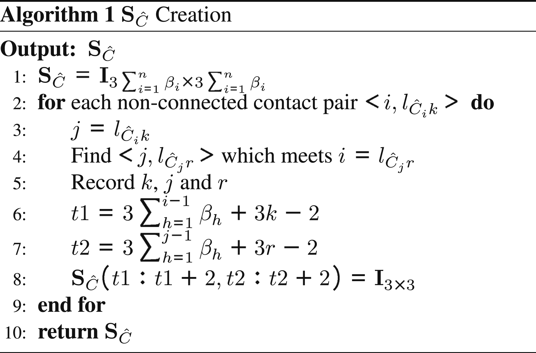
A non-connected contact between modules creates two local coordinate systems, each pointing from the contact point to the geometric center of its respective module. A matching matrix is required to constrain the forces following the Newton’s laws. Similarly to the connection, we create a matrix $S_{\hat{C}}$ to map the relationship between contact forces in different coordinate systems.

The creation algorithm has been shown in the Algorithm 1. For each non-connected contact pair, we locate the order number of the corresponding module by traversing all non-connected contact pairs and then adjust the $S_{\hat{C}}$ matrix. Since the contacts are mutual, the $S_{\hat{C}}$ matrix is symmetric. The simplest case involves only two non-connected contact modules. The two contact pairs are $< 1,2 >$ and $< 2,1 >$ . We take the two contact pairs into the “for” loop in Algorithm 1. The first contact pair $< 1,2 >$ makes t1 = 1 and t2 = 4, while the second contact pair $< 2,1 >$ makes t1 = 4 and t2 = 1. Thus, the $S_{\hat{C}}$ for only two non-connected contact modules is 2 × 2 block matrix, with each elements being I_3×3.

Considering the transformation of contact forces from the local coordinate system to the global coordinate system, we can conclude the mutual action equilibrium of non-connected contacts as

S_{\hat{C}} {\tilde{R}}_{\hat{C}} f_{\hat{C}}^{T} = 0 .

(23)

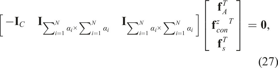
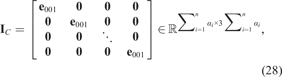
2.3.5. Decoupling equations of normal support force and adhesion force

Connectors provide an adhesion force that prevents the separation of connected modules, while the normal support force between the modules prevents their penetration. By decoupling the adhesion force and normal support force, we can isolate the connection force exerted solely by the connectors. This isolation is crucial for analyzing the required minimum connection strength to maintain configuration stability, as discussed in Section 3. Due to the mutual action equilibrium of connections, it is sufficient to consider the decoupling equations for child connections. We decouple the normal support force $f_{s_{i k}}$ at the connection point and z-axis adhesion force $f_{c o n_{i k}}^{z}$ from the connector in the local coordinate system. We use the subscript ik to indicate the k-th child connection of module i. Because the z-axis of the child connection coordinate system always points to the module’s interior region, $f_{s_{i k}}$ is always non-negative, while $f_{c o n_{i k}}^{z}$ is non-positive. For each child connection,

f_{A_{i k}}^{z} = f_{s_{i k}} + f_{c o n_{i k}}^{z},

(24)

where

f_{A_{i k}}^{z}

is the connection force along the z-axis direction. We note

f_{c o n_{i}}^{z} = [f_{c o n_{i 1}}^{z}, f_{c o n_{i 2}}^{z}, \dots, f_{c o n_{i α_{i}}}^{z}] \in R^{1 \times α_{i}},

(25)

and

f_{con}^{z} = [f_{c o n_{1}}^{z}, f_{c o n_{2}}^{z}, \dots, f_{c o n_{n}}^{z}] \in R^{1 \times \sum_{i = 1}^{n} α_{i}} .

(26)

f_s have the similar form as

f_{con}^{z}

. For each connection, we have the equation (24). Thus, the whole decoupling equation is

\begin{matrix} [\begin{matrix} - I_{C} & I_{\sum_{i = 1}^{N} α_{i} \times \sum_{i = 1}^{N} α_{i}} & I_{\sum_{i = 1}^{N} α_{i} \times \sum_{i = 1}^{N} α_{i}} \end{matrix}] [\begin{matrix} f_{A}^{T} \\ {f_{con}^{z}}^{T} \\ f_{s}^{T} \end{matrix}] = 0, \end{matrix}

(27)

where

I_{C} = [\begin{matrix} e_{001} & 0 & 0 & 0 \\ 0 & e_{001} & 0 & 0 \\ 0 & 0 & ⋱ & 0 \\ 0 & 0 & 0 & e_{001} \end{matrix}] \in R^{\sum_{i = 1}^{n} α_{i} \times 3 \sum_{i = 1}^{n} α_{i}},

(28)

\underset{Z}{\underset{⏟}{[\begin{matrix} {\bar{R}}_{A} & 0 & {\bar{R}}_{P} & 0 & {\bar{R}}_{C} & {\bar{R}}_{\hat{C}} & 0 & 0 \\ {\bar{P R}}_{A} & {\bar{R}}_{A} & {\bar{P R}}_{P} & {\bar{R}}_{P} & {\bar{P R}}_{C} & {\bar{P R}}_{\hat{C}} & 0 & 0 \\ {\tilde{R}}_{A} & 0 & S_{P} {\tilde{R}}_{P} & 0 & 0 & 0 & 0 & 0 \\ 0 & {\tilde{R}}_{A} & 0 & S_{P} {\tilde{R}}_{P} & 0 & 0 & 0 & 0 \\ 0 & 0 & 0 & 0 & 0 & S_{\hat{C}} {\tilde{R}}_{\hat{C}} & 0 & 0 \\ - I_{C} & 0 & 0 & 0 & 0 & 0 & I_{\sum_{i = 1}^{n} α_{i} \times \sum_{i = 1}^{n} α_{i}} & I_{\sum_{i = 1}^{n} α_{i} \times \sum_{i = 1}^{n} α_{i}} \end{matrix}]}} \underset{x}{\underset{⏟}{[\begin{matrix} f_{A}^{T} \\ m_{A}^{T} \\ f_{P}^{T} \\ m_{P}^{T} \\ f_{C}^{T} \\ f_{\hat{C}}^{T} \\ {f_{con}^{z}}^{T} \\ f_{s}^{T} \end{matrix}]}} = \underset{b}{\underset{⏟}{[\begin{matrix} - I_{e f} f_{e}^{T} \\ - {\bar{P}}_{e} f_{e}^{T} - I_{e m} m_{e}^{T} \\ 0 \\ 0 \\ 0 \\ 0 \end{matrix}]}}

(29)

and

e_{001} = [\begin{matrix} 0 & 0 & 1 \end{matrix}]

. All equilibrium equations have been considered above and we can conclude equations (6), (16), (20), (23), and (27) to form the compact matrix form as shown in equation (29). We use Zx = b to simplify the expression. It is worth noting that if each module is stable, the whole body must be stable. Therefore, we do not need to add extra constraints to ensure whole-body stability.

2.4. Friction cone constraints

The point contact model requires the contact forces to satisfy the friction cone constraints. The environmental contact friction cone is defined as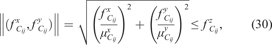

‖(f_{C_{i j}}^{x}, f_{C_{i j}}^{y})‖ = \sqrt{{(\frac{f_{C_{i j}}^{x}}{μ_{C_{i j}}^{x}})}^{2} + {(\frac{f_{C_{i j}}^{y}}{μ_{C_{i j}}^{y}})}^{2}} \leq f_{C_{i j}}^{z},

(30)

where

f_{C_{i j}}^{x}

f_{C_{i j}}^{y}

and

f_{C_{i j}}^{z}

are the x-axis, y-axis and z-axis components of

f_{C_{i j}}

in the local coordinate system ΣC_ij, respectively.

μ_{C_{i j}}^{x}

and

μ_{C_{i j}}^{y}

are the friction coefficient along the x-axis and y-axis in the local coordinate system, respectively. To simplify notation, we use

f_{C_{i j}} \in K_{C_{i j}} (μ_{C_{i j}}^{x}, μ_{C_{i j}}^{y}), i \in [1, n], j \in [1, γ_{i}],

(31)

to indicate that all environmental contact forces meets the friction cone condition.

K_{C_{i j}}

represents the friction cone constraint in the coordinate system. Similarly, the non-connected contacts are also expressed by the point contact model, the friction cone constraints are

f_{{\hat{C}}_{i u}} \in K_{{\hat{C}}_{i u}} (μ_{{\hat{C}}_{i u}}^{x}, μ_{{\hat{C}}_{i u}}^{y}), i \in [1, n], u \in [1, β_{i}],

(32)

where

K_{{\hat{C}}_{i u}}

is the friction cone constraint in the coordinate system

Σ {\hat{C}}_{i u}

μ_{{\hat{C}}_{i u}}^{x}

and

μ_{{\hat{C}}_{i u}}^{y}

are the corresponding friction coefficient in local coordinate system. The surface contacts can also be discretized into finite point contacts, so using the point contact model has general significance.

3. SOCP model and internal stability margin

In this section, we analyze the impact of the internal connector on the stability of MSRR. By formulating the SOCP problem, the critical stable state and internal stability margin can be obtained.

3.1. Connector constraint

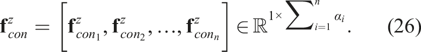
In Section 2, we derive the equilibrium equations and inequalities for the entire MSRR system to maintain stable. The solutions that satisfy equation (29) and the friction cone constraints (31)-(32) can ensure the system’s stability, provided that the internal connection constraints are sufficient. We first define the potential stable state set $X$ as follows.

Definition 1

Let an MSRR system composed of n modules be supported by frictional contacts against gravity and other known external wrenches in $R^{3}$ . The pot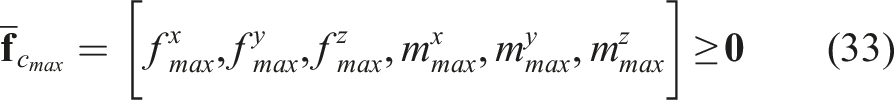ential stable state set $X$ comprises all solutions that satisfy the equilibrium equation (29) and friction cone conditions (31) and (32).

Note that $x \in X$ encompasses all connection wrenches and contact forces, as specified in equation (29). $X$ does not account for connector constraints, implying that all connection are assumed to be fixed. Under these conditions, the stability problem of MSRR degenerates into the problem of whole-body stability. The direct method to address connector constraints involves comparing whether solutions within $X$ meet the actual connector constraint range. We consider that the connector constraints in different dimensions are relatively uncoupled, as is often the case with mechanical connectors (White et al., 2011; Piranda et al., 2021). In cases where the coupling of connector constraints in different dimensions is strong, such as with magnetic connectors, further modeling of these coupling relationships can be conducted. The details of this modeling process are demonstrated in Section 5. We define

{\bar{f}}_{c_{\max}} = [f_{\max}^{x}, f_{\max}^{y}, f_{\max}^{z}, m_{\max}^{x}, m_{\max}^{y}, m_{\max}^{z}] \geq 0

(33)

as the maximum connection wrench for one specific connector. The six elements in

{\bar{f}}_{c_{\max}}

can be independently measured by appropriate experimental equipment, as illustrated in Figure 4. We further define

{\bar{f}}_{A_{i k}} = [f_{A_{i k}}^{x}, f_{A_{i k}}^{y}, f_{c o n_{i k}}^{z}, m_{A_{i k}}^{x}, m_{A_{i k}}^{y}, m_{A_{i k}}^{z}]

(34)

as the connection wrench of the k-th connection of module i. The symbols x, y and z in the top right corner represent the components of

f_{A_{i k}}

along different axes. It is worth noting that the third element in

{\bar{f}}_{A_{i k}}

is the adhesion force

f_{c o n_{i k}}^{z}

, rather than

f_{A_{i k}}^{z}

. Thus, the connector constraint can be denoted as

{\bar{f}}_{c_{\max}}^{-} \leq {\bar{f}}_{A_{i k}} \leq {\bar{f}}_{c_{\max}}^{+}, \forall i \in [1, n], k \in [1, α_{i}],

(35)

where

{\bar{f}}_{c_{\max}}^{-} = - {\bar{f}}_{c_{\max}} \leq 0

(36)

and

{\bar{f}}_{c_{\max}}^{+} = [f_{\max}^{x}, f_{\max}^{y}, 0, m_{\max}^{x}, m_{\max}^{y}, m_{\max}^{z}] \geq 0 .

(37)

[{\bar{f}}_{c_{\max}}^{-}, {\bar{f}}_{c_{\max}}^{+}]

is the connection wrench range for one connector. We follow the definition of the child connection coordinate system, where the z-axis points to the interior region of the module. The connector cannot provide a repulsive force along the z-axis. Thus, the third element of

{\bar{f}}_{c_{\max}}^{+}

is zero, while the third element of

{\bar{f}}_{c_{\max}}^{-}

cannot be zero because the connector can provide a adhesion force. Due to the mutual action equilibrium of the connection, there is no need to consider the parent connection. By incorporating these connector constraints into the original problem in Definition 1, we obtain the feasible stable state set as follows.

Definition 2

The feasible stable state set $X_{℧}$ comprises all potential stable states that satisfy the connector constraints (37).

Based on the above derivation and definitions, we can conclude Theorem 1.

Theorem 1

Let an MSRR system be supported by frictional contacts against gravity and other known external wrenches in $R^{3}$ . If the system is stable, $X_{℧}$ must not be empty, and the actual physical stable state $x_{f}^{*}$ must be in $X_{℧}$ . Conversely, if $X_{℧}$ is empty, the system must be unstable. Under quasi-static conditions, if $X_{℧}$ is not empty, the system is stable.

Proof. If the physical system is stable, it must satisfy the equilibrium equations, friction cone constraints, and connector constraints. Consequently, its actual physical stable state, $x_{f}^{*}$ , must be an element within $X_{℧}$ . As its converse proposition, if $X_{℧}$ is empty, the physical system must be unstable. Under quasi-static conditions, the passive connection constraints and contact forces accumulate from zero. Therefore, the system can maintain an equilibrium state only if the $X_{℧}$ is not empty.

Each feasible stable state $x_{f} \in X_{℧}$ is regarded as a weakly stable state in Pang and Trinkle (2000), because this state may be easily affected by minor external disturbances. For MSRR systems, since the recoverable nature of connector deformation, the connections between modules do not increase the system’s weak stability property; instead, the weak stability property still primarily depends on the external contact environment. A simple example is a sphere placed directly above a fixed sphere. Initially, the system is stable; however a minor external disturbance can cause the upper sphere to move. If the upper sphere is connected to the lower sphere by a connector, the system will remain stable under limited external forces due to the recoverability of the connection. Considerable research has been conducted on the stability of legged robots, including studies on contact surfaces (Rimon et al., 2008; Or and Rimon, 2017) and stability margin methods (Park et al., 2019). These research methods can be directly applied to the whole-body stability analysis of MSRR systems, as internal connections do not introduce additional weak stability property.

3.2. SOCP model

In the following part, we analyze how to evaluate the stability level of internal connections for MSRR systems, referred to as the internal stability margin. During this process, a systematic approach for stability detection of MSRR systems is proposed. We aim to achieve the following two goals by further analyzing the internal stability problem:

1. For stable configurations, we aim to maintain the system with strong internal stability to resist disturbances.

2. For unstable configurations, we can determine the required minimum connection wrench to maintain stability, allowing us to specifically enhance the connector’s capability or strengthen the structural rigidity at weak points.

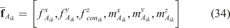
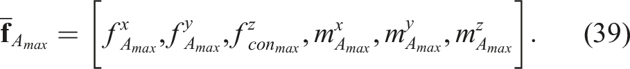
Without loss of generality, we assume that the modules in the MSRR system are all isomorphic, so the maximum connection wrench of the connectors is the same. We denote

f_{A_{\max}}^{x} = \max_{\binom{n \in [1, n]}{k \in [1, α_{i}]}} | f_{A_{i k}}^{x} |

(38)

as the maximum value of force along x-axis direction at all connection points. Similarly, the maximum values of forces or couples in other dimensions can also been obtained. Those values determine the minimum connection wrench required for the connector to reach the system’s state. Those values can be summarized as

{\bar{f}}_{A_{\max}} = [f_{A_{\max}}^{x}, f_{A_{\max}}^{y}, f_{c o n_{\max}}^{z}, m_{A_{\max}}^{x}, m_{A_{\max}}^{y}, m_{A_{\max}}^{z}] .

(39)

For each

x \in X

{\bar{f}}_{A_{\max}}

exists. Note that

{\bar{f}}_{c_{\max}}

in equation (33) is the actual values to express the maximum connection wrench for one specific connector, while

{\bar{f}}_{A_{\max}}

is the abstract mathematical concept to express the required minimum connection wrench to reach this state. If the actual connection wrench from the connector cannot exceed the required minimum connection wrench, the state cannot reach. The reachable state in

X

for the specific connector forms the feasible stable state set

X_{℧}

. We can plot the distribution of the required minimum connection wrench of each state x in a figure, using six dimensions of

{\bar{f}}_{A_{\max}}

as the coordinate. A two-dimensional case is shown in Figure 2, and we set

f_{A_{\max}}^{x}

and

m_{A_{\max}}^{y}

as variables. The red point in the Figure 2(a) represents the maximum connection wrench of the actual physical system. If the required minimum connection wrench of x exceed the red point at any dimension, this state is unreachable; otherwise, the state is reachable.

Figure 2.

The illustration of the internal stability margin.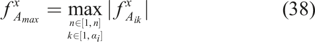

We move the red points and observe changes of $X_{℧}$ . When the red point moves toward the upper right corner, the number of elements in $X_{℧}$ increases. Conversely, when it moves towards the lower left corner, its number decreases rapidly. We use the black curve to denote the boundary where $X_{℧}$ will be empty if the red point falls below it. Due to the multidimensional nature of connector constraints, the curve is actually the Pareto frontier. When the system state moves on the boundary from left to right, the internal stress distribution within the system is also adjusting. The high requirement of $f_{A_{\max}}^{x}$ gradually decreases, shifting towards the demands on $m_{A_{\max}}^{y}$ , which demonstrates the mutual compensation effects of connections. It should be noted that when the red point is on the boundary, the number of elements in $X_{℧}$ can still be infinite if a null space exists for internal stress adjustments. All elements in the null spaces share the same values of ${\bar{f}}_{A_{\max}}$ .

If an MSRR system is stable in the absence of external disturbances, the actual state of the system, $x_{f}^{*}$ , is one element belonging to a corresponding feasible stable state set on the boundary. When external disturbances are present, the system deviates from the boundary state, requiring greater constraints to maintain stability. Thus, the distance from the boundary to the red point determines the anti-disturbance ability of the configuration. However, determining the shortest distance from the boundary to the red points is cumbersome and time-consuming, which is not conducive to the rapid calculation of internal stability margin.

In fact, physical systems in the real world converge towards a unique stable state, which is realized by harmonizing the displacements and deformations. When the constraints imposed by the connectors approach infinity, the actual state of the system is governed by the stiffness matrix of the connectors, placing the system in an optimally balanced load distribution state. Conversely, when the constraints of the connectors are insufficient, the system achieves the most balanced load distribution within the limits permitted by the connectors. We refer to this state as the critical stability state, which serves as our estimation of the system’s actual state. We define characteristic connection strength to evaluate the load distribution level of the system state.

Definition 3

The characteristic connection strength of a connection is given by

ω = {‖ω K {\bar{f}}_{A}‖}_{2},

(40)

where

{\bar{f}}_{A} \in R^{6}

is the 6-DOF connection wrench defined in equation (34),

K \in R^{6 \times 6}

is the matrix to represent the compliance of each dimensional force and torque.

ω \in R^{6}

is the weight coefficient to unify the dimension.

Note that ω and K are constant to represent the characteristics of a specific connector. The modeling method of ωK is not unique, as long as it can reflect the coupling relationship between connector constraints. For mechanical connectors, a typical choice of K is using the compliant matrix, which can be estimated by using the method in White et al. (2011). Thus, $K {\bar{f}}_{A}$ is the minor deformation of the connector under the connection wrench. ω can be set as the vector to unify the dimensions of displacement and rotation. For example, we can set ω = [1, 1, 1, ω₄, ω₅, ω₆] and the last three values equal to the moment arm to resist rotation along different axes. ω represents the resultant minor displacements. In Section 5, we demonstrate another method to determine ωK for magnetic connectors. Combing all we have defined and analyzed, we model the second-order cone program problem (41) to find the critical stable state.

\begin{aligned} \min λ_{\max} w_{A}^{\max} + λ_{1} \sum_{i = 1}^{n} \sum_{k = 1}^{α_{i}} w_{A_{i k}}^{\max} + λ_{2} \sum_{i = 1}^{n} \sum_{u = 1}^{β_{i}} f_{{\hat{C}}_{i u}}^{z} \\ + λ_{3} \sum_{i = 1}^{n} \sum_{j = 1}^{γ_{i}} f_{C_{i j}}^{z} \\ \begin{matrix} s . t . & Z x & = b, \\ - f_{s}^{T} & \leq 0, \\ {\bar{f}}_{A_{i k}} & \leq {\bar{f}}_{c_{\max}}^{+}, \\ - {\bar{f}}_{A_{i k}} & \leq - {\bar{f}}_{c_{\max}}^{-}, \\ w_{A_{i k}}^{\max} & \leq w_{A}^{\max}, \\ ‖ ω K {\bar{f}}_{A_{i k}} & ‖_{2} \leq w_{A_{i k}}^{\max}, \\ f_{C_{i j}} \in K_{C_{i j}} & (μ_{C_{i j}}^{x}, μ_{C_{i j}}^{y}), \\ f_{{\hat{C}}_{i u}} \in K_{{\hat{C}}_{i u}} & (μ_{{\hat{C}}_{i u}}^{x}, μ_{{\hat{C}}_{i u}}^{y}), \\ \forall i \in [1, n], j \in [1, γ_{i}], & u \in [1, β_{i}], k \in [1, α_{i}] . \end{matrix} \end{aligned}

(41)

The first term in the optimization objective is to minimize the maximum characteristic connection strength of all connections, fundamentally aiming to obtain the required minimum connection wrench to keep connection stable. The weight value of the first term, λ_max, is significantly larger than the other weights λ₁, λ₂, and λ₃. The second, third, and fourth terms in the objective function aim to minimize the sum of all characteristic connection strength, the sum of the non-connected contact forces along normal direction, and the sum of the environmental contact forces along normal direction, respectively. The last three terms are used for optimization within the null space of the vector space determined by the first term. The objective function can effectively eliminate the meaningless loss of internal constraints in the critical stable state but may lead to more potential broken connection points. When we are not concerned with the internal stress distribution within the configuration and only focus on the required minimum connection strength and stability margin, the optimization of the latter three terms can be omitted. The equilibrium equations, friction cone constraints and connector constraints are all incorporated in the optimization problem (41).

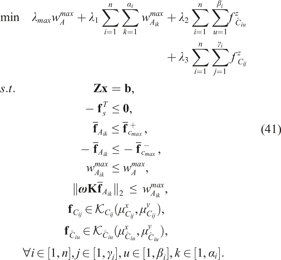
We denote $\tilde{x}$ to represent the critical stable state of the MSRR system. If the optimization problem (41) is solvable, $\tilde{x}$ is the optimal solution of it. Otherwise, $\tilde{x}$ is the optimal solution of the original optimization problem (41) removing the connector constraints. Based on $\tilde{x}$ , we can calculate the internal stability margin of the system and predict the broken connection points. The problem (41) can be quickly solved by modern solvers. Some specific adjustments of solvers can accelerate this process (Boyd and Wegbreit, 2007). Based on this, we can conclude Theorem 2.

Theorem 2

If an optimal solution for optimization problem ( 41 ) exists, the configuration of the MSRR system is stable. If the original optimization problem is infeasible and remains infeasible after removing the connector constraints, the configuration exhibits whole-body instability. Otherwise, the configuration exhibits internal instability.

Proof. If $X_{℧}$ is not empty, an optimal solution for problem (41) must exist. Using the Theorem 1, the system is stable. If we remove the connector constraints from the optimization problem (41), the search space is the potential stable state set $X$ . If the new problem is infeasible, the whole-body is unstable because the connection wrench is assumed to be infinitely rigid. Otherwise, the maximum connection wrench provided by the connector is insufficient to maintain the internal stability.

3.3. Internal stability margin

Once the critical stable state of the MSRR system is obtained, we can define the internal stability margin:

Definition 4

The internal stability margin for an MSRR system is given by

s_{s m} = m i n {\tilde{W} {\bar{f}}_{c_{\max}} - \tilde{W} {\tilde{f}}_{A_{\max}}},

(42)

where

{\bar{f}}_{c_{\max}}

is the maximum connection wrench for the specific connector and

{\tilde{f}}_{A_{\max}}

is the minimum connection wrench to reach the critical stable state

\tilde{x}

\tilde{W}

is the diagonal matrix to unify the dimensions of forces and couples.

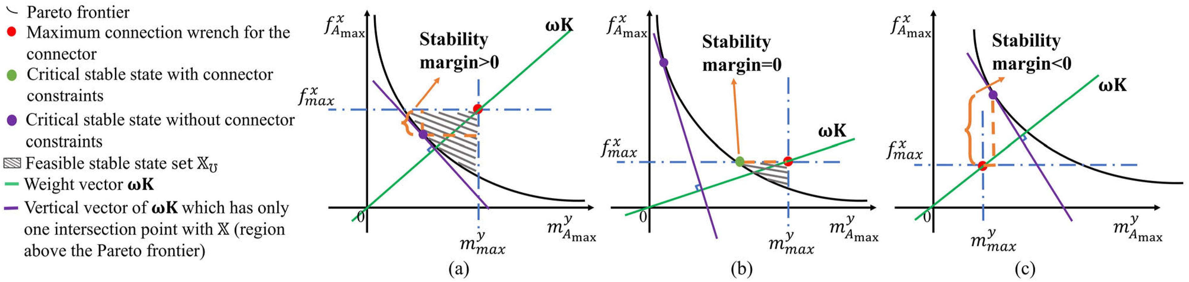
The internal stability margin is defined conservatively, which can ensure the effectiveness of indicators. We further illustrate the definition of internal stability margin combining Figure 2. Because only two variables are considered in Figure 2, the first term of optimization objective in problem (41) is:

\min ω_{1} m_{A_{\max}}^{y} + ω_{2} f_{A_{\max}}^{x},

(43)

where ω₁ and ω₂ are the weight values corresponding to

m_{A_{\max}}^{y}

and

f_{A_{\max}}^{x}

in ωK. Formula (43) essentially represents the inner product of two vectors, specifically the projection of the minimum connection wrench vector onto the weight vector. In Figure 2, the weight vector is depicted with a green line. Consequently, the point on the boundary line that has the shortest projection onto the weight vector, measured from the origin, corresponds to the solution set with the minimal maximum characteristic connection strength. If

X_{℧}

has unique solution, this state is the critical stable state. Otherwise, the critical stable state is determined by optimizing the last three terms in problem (41). When the connector constraints are not considered, the optimal solution takes into account the whole-body stability of the system and optimizes the load distribution based on the deformation characteristics of the connectors, as indicated by the purple point in Figure 2. When the actual connector constraints are considered, the optimal solution is marked with green points. It is evident that the green points are strictly confined within the region of

X_{℧}

In Figure 2(a), the green and purple points coincide, and according to Definition 4, the internal stability margin is the shorter of the two orange dashed lines. In Figure 2(b), the purple point does not lie within $X_{℧}$ , indicating that the state represented by the purple point is unreachable. In this case, the green point corresponds to the solution set that is closest to the purple point within $X_{℧}$ . The internal stability margin is defined as zero because the constraints in certain dimensions are at their limits. In Figure 2(c), we consider the case where the actual connection constraints are insufficient, resulting in $X_{℧} = \emptyset$ . If the configuration is whole-body stable, we can obtain the critical stable state without considering the connector constraints. The internal stability margin can be obtained by measuring the maximum difference between the red and purple points in all constraint dimensions, and its value is negative. In Definition 4, $\tilde{W}$ is used to unify the dimensions of forces and couples; its diagonal elements can be set to [1,1,1,1/ω₄,1/ω₅,1/ω₆] for mechanical connectors, where the last three values are the reciprocals of the moment arm of couples. To discuss the internal stability margin more intuitively, the influence of the weight is not shown in Figure 2. Further, we define potential broken connection points as follows.

Definition 5

For each connection in the critical stable state $\tilde{x}$ , if

w_{A}^{\max} - ‖ ω K {\bar{f}}_{A_{i k}} ‖_{2} \leq ϵ, i \in [1, n], k \in [1, α_{i}],

(44)

where ϵ is positive and close to 0, this connection is the potential broken connection point.

4. Quasi-static stability algorithm

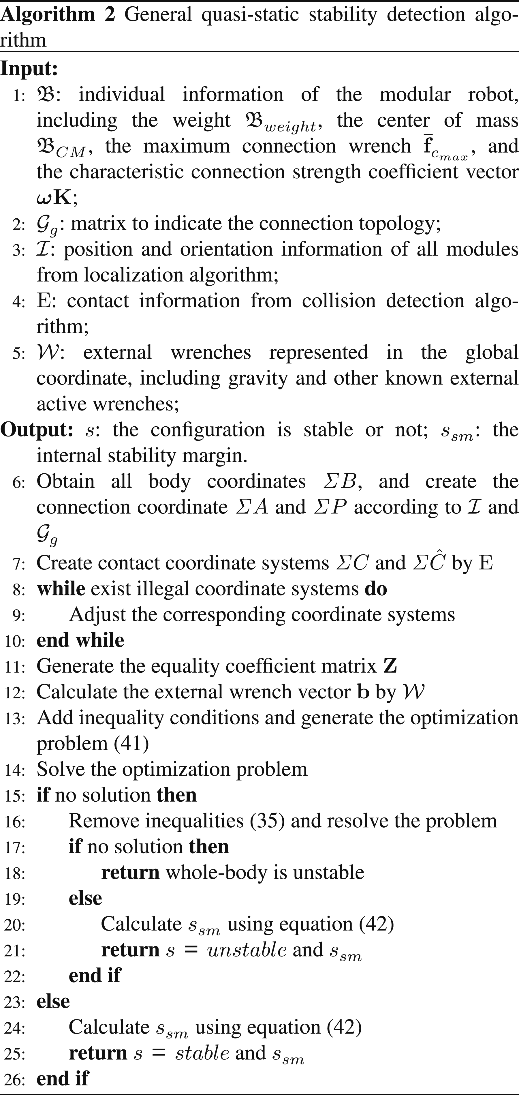
The general quasi-static stability detection algorithm is proposed here in order to completely present how to use the above model to realize fast stability detection. The algorithm is concluded in Algorithm 2.

4.1. Model construction and algorithm input

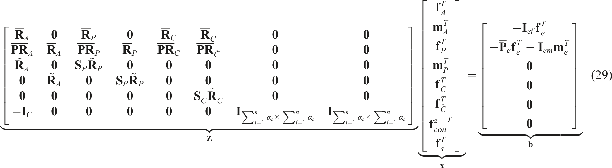
The core of the detection algorithm proposed in this paper is to construct the SOCP problem (41). This optimization problem can be quickly solved by modern solvers, as demonstrated in section 6.4. Therefore, we do not engage in extensive discussion regarding the problem solving. The SOCP problem (41) involves a considerable number of parameters, but fortunately, most of the information can be obtained in advance. In this subsection, the inputs required for the algorithm are first discussed.

We first observe the equation (29). The constant matrix Z on the left side of the equation includes the position and orientation information of the body coordinate system, the connection coordinate system, and the contact coordinate system. The constant vector b on the right side of the equation describes the external wrenches acting on each module, including gravitational forces and torques. Additional required parameters include the maximum connection wrench range ${\bar{f}}_{c_{\max}}$ for the specific connector and the coefficient vector ωK for characteristic connection strength. The values of ${\bar{f}}_{c_{\max}}$ can be determined using instruments similar to those shown in Figure 4, while ωK can obtained through experimental methods as shown in White et al. (2011) or other method as if it can reflect the coupling relationships between connector constraints. Therefore, the reminder problem is how to construct Z and b. We introduce the steps involved in constructing the equation (29) and discuss the relevant algorithm inputs during this process.

Step 1: Define the body coordinate system and the connection coordinate system of two connected module. Typically, the body coordinate system is positioned at the geometric center of the module, while the connection coordinate system is established at the connection point.

Step 2: Allocate IDs to the modules and construct a connection relationship matrix $G_{g}$ to represent the connectivity topology. The value in the i-th row and j-th column of the matrix represents the relationship between module i and module j. For module i, the parent connection of module j is marked as “2,” and the child connection as “1.”

Step 3: Based on the localization algorithm or forward kinematic model, obtain the transformation matrix of the module body coordinate system and the connection coordinate system in the global coordinate system for the configuration.

Step 4: Based on collision detection method to generate the corresponding contact coordinate systems.

Step 5: Check that all connection and contact coordinate systems conform to the direction definitions provided in Section 2 and create the matrix Z.

Step 6: Consider known external forces, such as gravity, to construct vector b.

As shown in Algorithm 2, although the input includes multiple types, the quasi-static stability detection algorithm, which runs subsequent to the localization and collision detection algorithms, can easily obtain the necessary kinematic and contact relationships. Even for modular robots with complex, irregular shapes, the positions of contact points can be identified through effective collision detection algorithms. Therefore, it does not require excessive effort to implement this algorithm. Furthermore, inaccuracies in the positioning and orientation of coordinate systems can lead to deviations in the acting positions of constraints, which in turn can result in shifts in the predicted outcomes. Additionally, imprecise measurements of connector constraints may also yield inaccurate results. Therefore, configurations with a larger stability margin are preferred, as they enhance the system’s ability to tolerate input errors and external disturbances.

Note that the system’s interactions with different objects are distinct in the model, and here we make specific distinctions. The first type involves interactions with the environment, including the ground and walls. These interactions are represented through environmental friction cones. The second type involves interactions with objects subjected to gravity, where such objects can be considered as one type of module, maintained in stability solely through non-connected contacts, such as the box in Figure 6(b). The third type involves interactions with targets that actively exert wrenches. The wrench source could be the weight of a point mass or a device capable of applying a constant wrench. Gravity is considered a typical known external force, whereas forces exerted by human fingers or other mechanical manipulators are difficult to predict. An effective approach is to assume an external force at a certain point in the configuration and repeatedly solve optimization problems using a method similar to binary search to determine the acceptable range of external forces at that point.

4.2. Algorithm output

The optimization problem (41) can be easily solved using a commercial solver. If the solution exists, the internal stability margin is not negative and the configuration is stable. We can get all connection wrenches at each connection point. Otherwise, the configuration is unstable, and we can remove the connector constraints to further determine the unstable reasons. If the solution also does not exist, the whole-body is unstable. Otherwise, the maximum connection wrench provided by the connector is not enough and we can know the internal stress distribution of the configuration based on the critical stable state, which can guide us in designing the hardware and choosing suitable configurations.

5. Algorithm application

The quasi-static stability detection algorithm we proposed is applied to the FreeSN system. We introduce the hardware platform utilized in our experiments and further address the coupling relationships among FreeSN connector constraints. Simulation analysis of two configurations composed of numerous FreeSN modules are also carried out in this section.

5.1. FreeSN mechanism and forward kinematics

The modular reconfigurable robot, FreeSN, depicted in Figure 3, consists of two main components: node and strut. The node is an iron spherical shell equipped with a magnetic sensor array, while the strut, a two-wheeled vehicle, connects to the node via bottom magnets (Tu et al., 2022). Unlike the node, which cannot move by itself, the strut can attach to any point on the node and move across its surface by controlling an internal motor. Additionally, the strut features a magnet lifting mechanism that facilitates the attachment and detachment of the node. Collectively, the FreeSN system can configure into various serial or parallel mechanical structures, supporting multiple locomotion types.

Figure 3.

The coordinate system of FreeSN.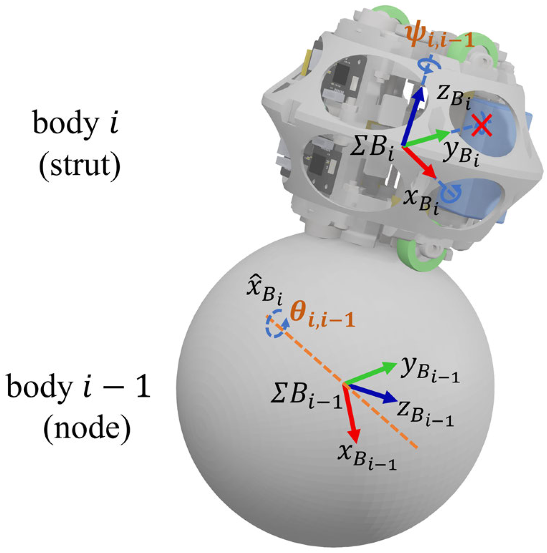

We develop the forward kinematic model for FreeSN in the position domain, which facilitates the generation of coordinate systems and form different MSRR configurations. Specifically, we consider a configuration where one node is connected to a strut. As depicted in Figure 3, ΣB_i and ΣB_i−1 represent the coordinate systems attached to module i and module i − 1, respectively. The z-axis of ΣB_i consistently points from the geometric center of module i − 1 to the geometric center of module i. The initial rotation matrix of the coordinate system ΣB_i with respect to ΣB_i−1 is denoted as ${}^{B_{i - 1}}R_{B_{i}}$ . The strut can realize the rotation around the $z_{B_{i}}$ direction by the differential wheels and rotate around the $x_{B_{i}}$ direction. The new orientation and position of the strut can be calculated by the equations (45) and (46):

{}^{B_{i - 1}}{\tilde{R}}_{B_{i}} = {}^{B_{i - 1}}R_{B_{i}} R_{z} (ψ_{i, i - 1}) R_{x} (θ_{i, i - 1}),

(45)

{}_{B_{i - 1}}^{B_{i - 1}}{\tilde{p}}_{B_{i}} = l_{i - 1} {\tilde{z}}_{B_{i}},

(46)

where

{}^{B_{i - 1}}{\tilde{R}}_{B_{i}}

represents the rotation matrix of ΣB_i with respect to ΣB_i₋₁ after movement. The strut first rotates ψ_i,i₋₁ around the z-axis of the coordinate system ΣB_i, followed by a rotation of θ_i,i₋₁ around the x-axis of the new coordinate system. R_z and R_x denote the elementary rotation matrices about the z-axis and x-axis of the frame, respectively. The new position of ΣB_i, denoted by

{}_{B_{i - 1}}^{B_{i - 1}}{\tilde{p}}_{B_{i}}

, is uniquely determined by its rotation matrix, where

{\tilde{z}}_{B_{i}}

is the third column of

{}^{B_{i - 1}}{\tilde{R}}_{B_{i}}

and l_i₋₁ represents the distance from the center of the node to the center of the strut.

5.2. Connection mode and model construction

For connectors with relatively decoupling relationship between constraints, the connector constraints are represented as in inequality (35), which actually defines a six-dimensional cube. For connectors like FreeSN, complex coupling relationship exists between connector constraints. Further modeling and analysis of its connectors are required. The strut and node are connected by magnets. The magnetic force strengthens the attachment along the z-axis in the local coordinate system, providing powerful constraints to impede the position and rotation of modules. Therefore, the connection method of FreeSN can be seen as a magnetically enhanced contact model, and we can model the coupling relationships between its constraints based on a six-dimensional Lorentz cone. The definition of the Lorentz cone is as follows,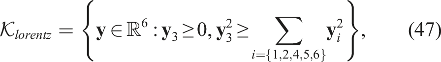

K_{lorentz} = \{y \in R^{6} : y_{3} \geq 0, y_{3}^{2} \geq \sum_{i = {1,2,4,5,6}} y_{i}^{2}\},

(47)

where y represents a parameter vector, and the subscript denotes the element’s position within the vector. For each connection of FreeSN, the inequality (47) holds and can be written as

\begin{matrix} {\bar{f}}_{s_{i k}} (μ) \in K_{lorentz}, \forall i \in [1, n], k \in [1, α_{i}], \end{matrix}

(48)

where

{\bar{f}}_{s_{i k}} (μ) = [\frac{f_{A_{i k}}^{x}}{μ_{1}}, \frac{f_{A_{i k}}^{y}}{μ_{2}}, f_{s_{i k}}, \frac{m_{A_{i k}}^{x}}{μ_{4}}, \frac{m_{A_{i k}}^{y}}{μ_{5}}, \frac{m_{A_{i k}}^{z}}{μ_{6}}]

(49)

is the connector constraint vector of FreeSN, and μ = [μ₁, μ₂, μ₄, μ₅, μ₆] is the coefficient vector to reflect the coupling relationship between connector constraints of FreeSN. It is worth noting that the third element in

{\bar{f}}_{s_{i k}}

is the normal support force

f_{s_{i k}}

. The connector constraints of FreeSN can be represented by inequalities (48). We set ωK = [1/μ₁, 1/μ₂, 1, 1/μ₄, 1/μ₅, 1/μ₆]. According to formula (24) and (48), we obtain

\begin{matrix} {‖ω K {\bar{f}}_{A_{i k}}‖}_{2}^{2} \leq {(f_{A_{i k}}^{z} - f_{c o n_{i k}}^{z})}^{2} + {(f_{c o n_{i k}}^{z})}^{2} \end{matrix},

(50)

where

f_{c o n_{i k}}^{z}

is negative and

f_{A_{i k}}^{z}

is the value determined by the external wrenches. Thus, the inequality (50) shows that minimizing

w_{A}^{\max}

in problem (41) is same as minimizing

- f_{c o n_{i k}}^{z}

for FreeSN. The minimum characteristic connection strength optimization problem for FreeSN can be reorganized as (51)

\begin{aligned} \min λ_{\max} f_{\max} + λ_{1} \sum_{i = 1}^{n} \sum_{k = 1}^{α_{i}} (- f_{c o n_{i k}}^{z}) + λ_{2} \sum_{i = 1}^{n} \sum_{u = 1}^{β_{i}} f_{{\hat{C}}_{i j}}^{z} \\ + λ_{3} \sum_{i = 1}^{n} \sum_{j = 1}^{γ_{i}} f_{C_{i j}}^{z} \\ \begin{matrix} s . t . & Z x & = b, \\ - f_{c o n_{i k}}^{z} & \leq f_{\max}, \\ {\bar{f}}_{s_{i k}} (μ) & \in K_{lorentz}, \\ f_{C_{i j}} \in K_{C_{i j}} & (μ_{C_{i j}}^{x}, μ_{C_{i j}}^{y}), \\ f_{{\hat{C}}_{i u}} \in K_{{\hat{C}}_{i u}} & (μ_{{\hat{C}}_{i u}}^{x}, μ_{{\hat{C}}_{i u}}^{y}), \\ \forall & i \in [1, n], j \in [1, γ_{i}], & u \in [1, β_{i}], k \in [1, α_{i}] . \end{matrix} \end{aligned}

(51)

Note that the value of λ_max is significantly larger than other weights. The internal stability margin equation is

s_{s m} = f_{\max}^{z} - f_{\max}^{*},

(52)

where

f_{\max}^{z}

is maximum connection force from FreeSN connectors and

f_{\max}^{*}

is the minimum value of f_max in problem (51).

5.3. Experimental devices and parameter measurement

We demonstrate the method we used to measure the connector parameters. The platform to measure related parameters is shown in Figure 4. A white shell is installed on a strut module. Some drawstrings can through the shell to apply external force. A hemisphere base is the node module and the strut is connected with it. The location of the strut and node is varied according to the parameter we want to measure. A force gauge is fixed on the slide rail, which is controlled by a handle.

Figure 4.

Experimental equipment to obtain 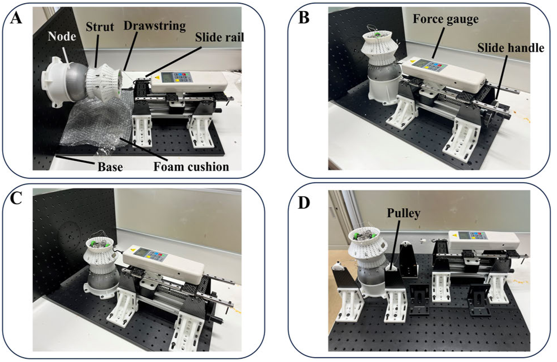${\bar{f}}_{c_{\max}}$ of FreeSN. (A) normal force measurement, corresponding variable $f_{\max}^{z}$ in equation (33); (B) shear force measurement, corresponding variables $f_{\max}^{x}$ and $f_{\max}^{y}$ ; (C) bending moment measurement, corresponding variables $m_{\max}^{x}$ and $m_{\max}^{y}$ ; (D) torsional moment measurement, corresponding variable $m_{\max}^{z}$ .

In Figure 4(a), the maximum connection force along the z-axis, $f_{\max}^{z}$ , can be measured by rotating the handle and recording the value on the screen when the connection breaks. The height of the base node is different in the Figure 4(b) and (c). We test the shear force along different directions in the tangential plane in (B) and test the bending torque in (C). Thus, the values, $f_{\max}^{x}$ , $f_{\max}^{y}$ , $m_{\max}^{x}$ and $m_{\max}^{y}$ , can be obtained. Extra pulley blocks are utilized in (D) to calculate the value of $m_{\max}^{z}$ which represents the resistance capacity of the connector when a pure torsional moment is applied. Thus, the maximum connection wrench of FreeSN, ${\bar{f}}_{c_{\max}}$ , is obtained and the coefficient vector μ of the Lorentz cone can be obtained as

μ = [\frac{f_{\max}^{x}}{f_{\max}^{z}}, \frac{f_{\max}^{y}}{f_{\max}^{z}}, \frac{m_{\max}^{x}}{f_{\max}^{z}}, \frac{m_{\max}^{y}}{f_{\max}^{z}}, \frac{m_{\max}^{z}}{f_{\max}^{z}}] .

(53)

5.4. Simulation analysis

In this section, we conduct the simulation analysis of the algorithm. The MSRR system, constituted by FreeSN, forms suspension and object manipulation configurations. We use the parameters from the actual physical system in the simulation process. The weight and height of a strut module are 492 g and 87 mm, respectively. The weight and radius of a node module are 361 g and 60 mm. The parameter of the characteristic connection strength for FreeSN, as shown in equation (53), can be measured by the equipment in Figure 4. Each strut is the same with μ = [0.2838, 0.2483, 0.0071, 0.0083, 0.0043]. We set λ_max = 10,000 and λ₁ = λ₂ = λ₃ = 1 in optimization problem (51). FreeSN achieves connection through pure magnetic forces. The optimization of characteristic connection strength of FreeSN is equivalent to minimize the magnetic force, as shown in formula (50). In the following part, we use “connection force” to represent the required magnetic forces at connection points. As shown in Figures 5 and 6, the algorithm proposed in this paper is applied to analyze two configurations: suspension and object manipulation. The internal stress distribution depicted in the figures represents the system’s critical stable state obtained by solving the optimization problem (51). We use different colors to illustrate the required connection force at each connection point. All optimization problems are solved using the CVX solver (Michael Grant and Stephen Boyd).

Figure 5.

The stress distribution at the connection points of a suspension configuration composed of 76 FreeSN modules. (a) Before the disconnection, the configuration is uniformly stressed under gravity and requires a maximum of only 76.5 N of magnetic force to maintain stability. (b) After the disconnection, at least 948.4 N magnetic forces are required to maintain stability. (c) Normal force distribution after the disconnection. (d) Shear force distribution after the disconnection.

Figure 6.

The stress distribution at the connection points in an object manipulator configuration, which is composed of 73 FreeSN modules, under the influence of load gravity and external force.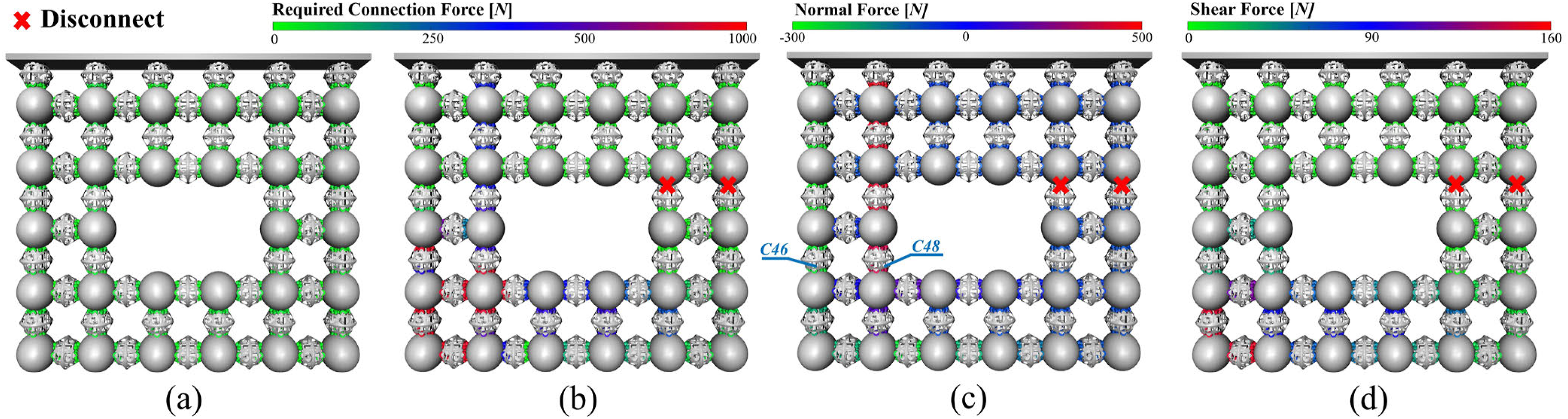

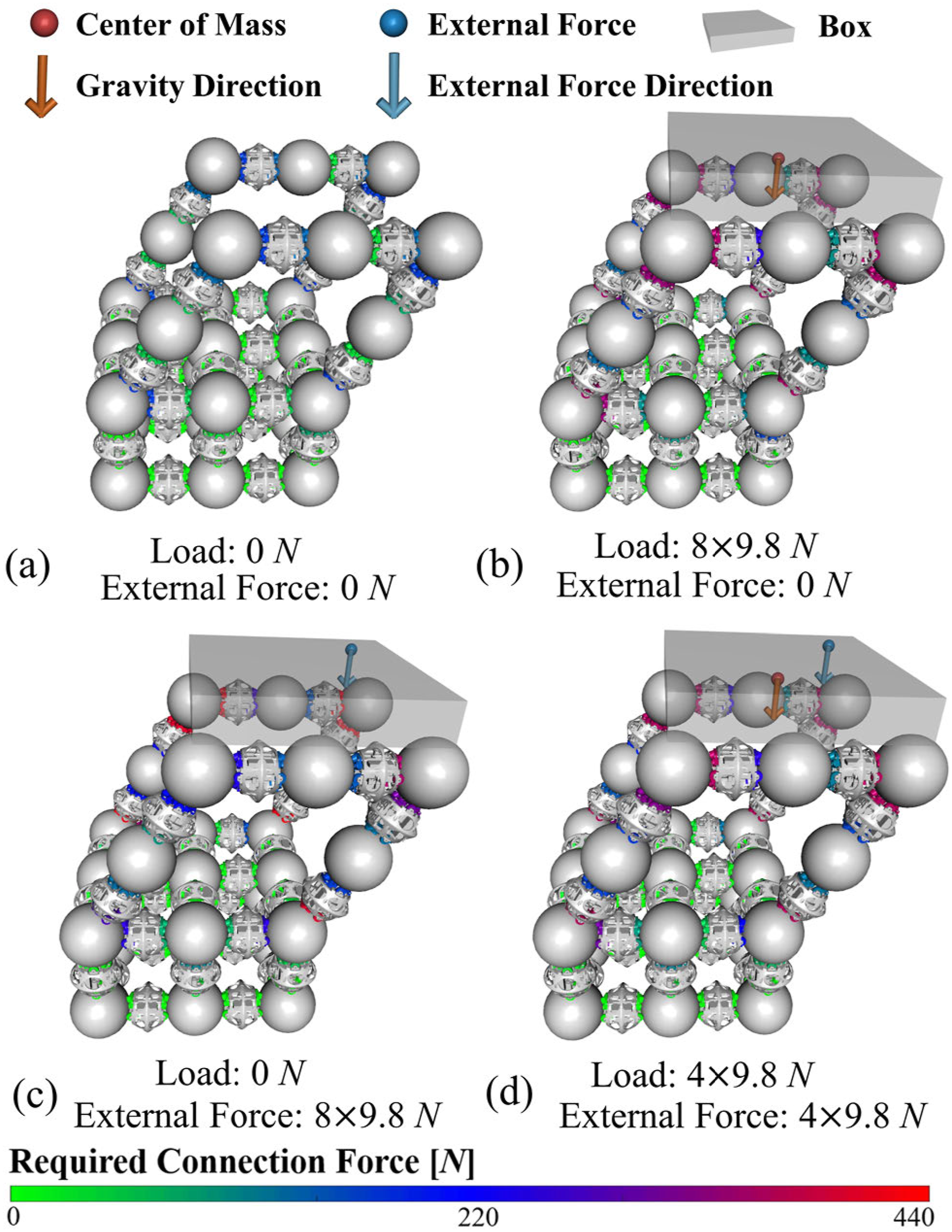
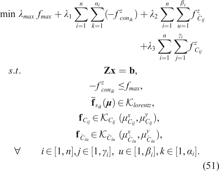
Figure 5 shows a suspension configuration composed of 76 FreeSN modules under gravity, with the top struts fixedly connected to the wall. By solving the optimization problem (51), the critical stable state of the system can be obtained, and the required connection force at each connection point can be obtained. In Figure 5(a), the gravity of the modules is uniformly distributed, and the entire configuration can be stable with just 76.5 N of connection force. In Figure 5(b), after disconnecting the two connection points, the modules in the lower left corner are required to provide substantial shear forces and rotational torques to resist the gravity. The required minimum connection force increases to 948.4 N. The red connections in Figure 5(b) indicate potential broken connection points. In Figure 5(c), we illustrate the magnitude of the normal forces at each connection point. Notably, the column that includes the connection point “C48” demands a significantly higher normal force, in contrast to the relatively lower requirement at connection point “46.” The normal forces at these two connection points are in opposite directions, providing a couple to resist the rotation of the rest modules. In Figure 5(d), the modules in the lower left corner need to exert a substantial shear force to counteract the gravity of the modules on the right.

Figure 6 illustrates an object manipulation configuration consisting of 73 FreeSN modules, where the bottom layer’s nodes are fixed. This configuration facilitates the manipulation of an external object via a supporting platform at the top. During the modeling process, the load box is considered as one of the modules comprising the configuration, with considerations for force equilibrium, torque equilibrium, friction cone constraints, unconnected contacts and minimization of contact forces. This approach enables the configuration to interact with static external objects. We also demonstrate the effects of external active forces applied to the system. The action points, directions, and magnitudes of the active external forces are given and are incorporated into vector b of equation (29). Figure 6(a) displays the system configuration and the distribution of required connection forces under conditions without load and external forces. The system requires a minimum of 171.48 N of magnetic force to maintain stability. In Figure 6(b), an 8 kg box is placed on top of the system, and it can be observed that the gravitational force of the load is evenly distributed to the internal connections, with the largest compression occurring at the four connection corners. The system requires a minimum 355.1 N magnetic force to maintain the connections. In Figure 6(c), we assume the box is light enough to be negligible; applying external force at a point on the box shows that the internal stress is more heavily loaded on the side closer to the action point of the external force. The required minimum connection force is 425.39 N. In Figure 6(d), the box gravity and external force are the same, and the required minimum connection force is 364.01 N.

The simulation experiments presented above demonstrate the application and effectiveness of the algorithm in complex scenarios. The critical stable states achieved are consistent with the natural properties of load distribution.

6. Experiments

We carried out comprehensive physical experiments to test the modeling accuracy and algorithm usability, including motion range comparison, configuration experiments, and a load experiment. We also analyze the calculation efficiency of our method in this section. We use the same parameters of FreeSN as introduced in Section 5.4, unless otherwise specified.

6.1. Motion range comparison

A series of FreeSN modules compose a manipulator as shown in Figure 7. By moving the bottom strut on the node, we can obtain the stable motion range of the bottom strut. Comparing it with our numerical results, we can know the accuracy of our modeling. The coefficients μ varies with the change of the height of magnets. We tested the connection strengths of the bottom strut, and then obtained μ = [0.2413, 0.2201, 0.0054, 0.0064, 0.0023]. The maximum magnetic force is 104.5 N.

Figure 7.

(a), (b), and (c) show the motion range comparisons between the numerical results and the physical samples for different manipulator configurations. The bright blue region represents the calculated stable region, while the gray region indicates instability. Blue triangles denote stable samples, and red triangles represent unstable samples in physical systems.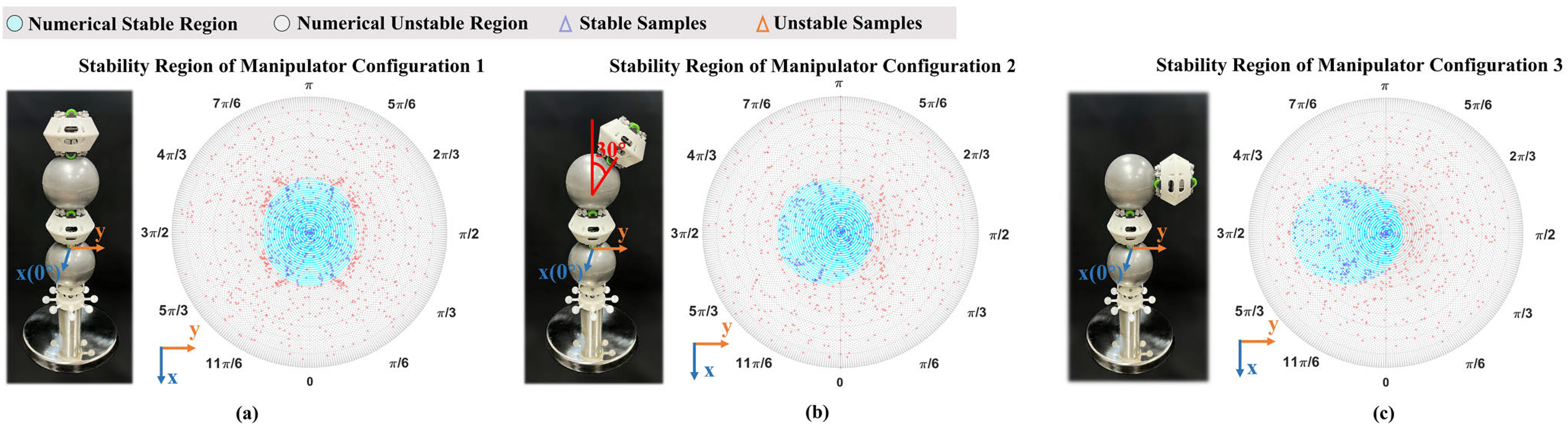

As shown in Figure 7, a base node was connected by two struts and one node. We fixed the top strut and its angles related to its connected node were set as 0°, 30°, and 90°, respectively. We controlled the bottom strut moving on the node and kept its y-axis of the contact coordinate system aligned with its original direction. The numerical prediction results obtained from the proposed model are represented by bright blue and gray points in Figure 7. The bright blue point indicates stable configurations, while the gray points denote instability. In Figure 7(a), the blue region is elliptical because the rubber tires in the x direction have a higher coefficient of friction compared to the universal wheels in the y direction, which have a lower friction coefficient. In Figure 7(b)-(c), the shape of the bright blue region becomes irregular due to the positional change of the top strut. The region to the right of the base node is prone to falling.

We sampled many points by keeping the top strut fixed and moving the bottom strut randomly. The connection positions of the bottom strut in the polar coordinate system were recorded using the localization method introduced in Tu and Lam (2023). The orientation error of this method is approximately 1°. If the system was unstable, we recorded it as 0; if stable, it was recorded as 1. In Figure 7, the blue triangles represent stable samples, and the red triangles indicate unstable ones. Theoretically, the blue triangles should be located within the bright blue region, while the red triangles lie within the gray region. We sampled a total of 1128, 867, and 880 points for three different manipulator configurations, respectively. We found that the boundaries between the red and blue sampling points are close to the numerical calculation boundaries. Few outliers exist around the boundary, resulting from localization errors and possible wear of the rubber tires. Although this is the simplest configuration, we can conclude that the point contact model, Lorentz cone model, and other settings are sufficiently accurate, and our modeling and algorithm process have been effectively verified.

6.2. Configuration experiments

A series of physical experiments utilizing FreeSN were conducted to demonstrate the usability of the method proposed in this paper. The MSRR system, constructed by FreeSN, formed different configurations, including open-chain and closed-chain types on both even and uneven floors. By analyzing those experiments, we find that although the method proposed in this paper is based on simple criteria, it still provides sufficient prediction accuracy and instability information. Details of the dynamic process involved in the configuration experiments are available in the supplemental video.

As shown in Figure 8, six different configurations were constructed using FreeSN, and our method was utilized to predict the stability of each configuration and identify the unstable connection points. We only optimize the maximum characteristic connection strength of the configuration, which is the first optimization objective in problem (51). By adjusting the height of magnets, we ensured that the connection strength of each strut was uniform, with μ = [0.2838, 0.2483, 0.0071, 0.0083, 0.0043], and the maximum magnetic force was 109.2 N. The friction coefficient of the ground and steps are 0.8 and 0.26, respectively. Those parameters were also used in Section 6.3. The position and orientation of all modules were recorded by a motion capture system, and the relative motion between modules can help us analyze the real unstable connections. The mean error of the motion capture system is 0.312 mm during the calibration, which decides the measurement uncertainty. In Figure 8, column (a) illustrates the initial configuration. The color of each connection point, labeled as “C#,” represents the degree of stress. By solving the optimization problem (51), we can obtain the required minimum connection force $(f_{\max}^{*})$ of this configuration, and obtain the required connection wrench at each connection point. We can determine whether the configuration is stable by using s_sm or Theorem 2. The external contact friction margins were also calculated by subtracting the left side of inequality (30) from its right side, which is labeled as “S#” in Figure 8. Column (b) shows the stress distribution of the configuration after adding the new module or loads. If the required minimum connection force exceeds the connection force provided by the struts, the configuration is unstable, and the overstressed connection points are marked by colors ranging from purple to red. Column (c) shows the outcomes of the physical experiments, and the entire motion process was recorded by the motion capture system. We obtained the relative motion of the modules, allowing us to identify which connection points were broken. We extracted the motion at one instantaneous moment. The relative motion between modules is shown in column (d) of Figure 8 and is marked using orange bars. Since the accelerations at the broken points are very small, the breaking process is relatively slow. The light blue bars and dark blue bars represent the required connection wrench at each connection point before and after adding loads, respectively. The orange line represents the physical connection force from the connector. We can find the required minimum connection force is always higher than the physical connection force after adding the new module or loads, indicating that the configuration is unstable. We summarize the comparison results between predictions and experiments in Table 2.

Figure 8.

Six configuration experiments on FreeSN. (a) The theoretical results calculated using the proposed method before adding loads are shown. Colors at connection points represent the required connection forces; (b) the theoretically calculated results using our method after adding loads; (c) the states of the physical system after adding loads; (d) the required connection force at each connection point obtained from our model and the relative motion between modules after adding loads, as captured by a motion capture system.

Table 2.

The Numerical Results and Stability State of Different Configurations in Figure 8.

	Add loads	Theoretical results				Experimental results
	Add loads	Status	MCF (N)	s_sm (N)	Unstable point	Status	Unstable point
Con.#1	Before	Stable	105.228	3.972	∖	Stable	∖
	After	Unstable	122.357	−13.157	C8, C10, C11	Unstable	C8, C10
Con.#2	Before	Stable	88.4167	20.7833	∖	Stable	∖
	After	Unstable	124.619	−15.419	C8, C10, C11	Unstable	C8, C10
Con.#3	Before	Stable	104.886	4.314	∖	Stable	∖
	After	Unstable	134.753	−25.553	C3, C4, C7, C8, C12, C15	Unstable	C4, C7
Con.#4	Before	Stable	104.568	4.632	∖	Stable	∖
	After	Unstable	137.1	−27.9	C5, C7, C11	Unstable	C5, C11
Con.#5	Before	Stable	91.9152	17.2848	∖	Stable	∖
	After	Unstable	114.062	−4.862	C4, C8, C9,C12, C13	Unstable	C8, C12
Con.#6	Before	Stable	104.689	4.511	∖	Stable	∖
	After	Unstable	111.8591	−2.6591	C20, C22	Unstable	C20, C22

Con.# is consistent with the configuration in Figure 8. MCF means the required minimum connection force to maintain stability.

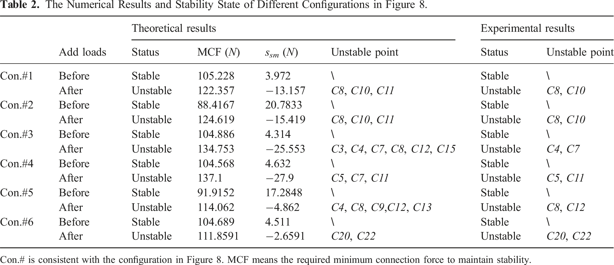
The initial configuration 1 was stable with a small stability margin. After adding the extra node, we can observe the instability of the configuration in Figure 8-#1c. We use Figure 8-#1c to represent the first row of column (c) and #1 is the abbreviation of Configuration#1. We follow this rule to refer to the specific figure. The relative motion in Figure 8-#1d points out that the connections “C8” and “C10” are first broken. In Figure 8-#1b, the connection “C8,” “C10,” and “C11” are predicted to be the most vulnerable broken points, consistent with the physical system. The potential broken connection points for Configuration#1 do not change before and after adding the new module as shown in Figure 8-#1d. Configuration#2 is similar to Configuration#1 and only the position of the added module is different. Before adding the extra module, Configuration#2 is stable, with 88.4167 N required minimum connection force, as shown in Figure 8-#2a. After adding one module, several overstressed connection points are shown in Figure 8-#2b. “C8,” “C10,” and “C11” are the easiest broken connection points and this can be verified from the orange bar in Figure 8-#2d, where the relative motion “C9” was caused by the motion of “C8” and “C10.” The real broken points observed by the motion capture are always included in the predicted potential broken points which can be observed in Table 2.

Compared the Configuration#1 and Configuration#2, we can find that the position of the extra module can greatly affect the distribution of internal stress. In Configuration#1, the extra module is added along the gravity direction which requires the bending torque. But in Configuration#2, the torsional constraint is required due to the positional change of the added module. Even though only one extra module is added in Configuration#2, the required minimum connection force increases from 88.4167 N to 124.619 N, and the required connection forces at “C1” and “C2” also greatly increase. It shows that the position of added modules has a large effect on configuration.

Configuration#3 is a closed-loop configuration and has a similar topology with the Test#6 in Piranda et al. (2021), where their proposed method failed to predict the broken connection points. Before adding the new module, Configuration#3 was predicted to be stable with the required minimum connection force 104.886 N. The addition of the new module caused the configuration instability because the required minimum connection force 134.753 N is greater than the connection force 109.2 N provided by the physical system. The experimental outcomes in Figure 8-#3c verified the result. In Figure 8-#3b, the connection points “C3,” “C4,” “C7,” “C8,” “C12” and “C15” have close stress levels, and connection points “C4” and “C7” are the real broken points according to Figure 8-#3d. Besides, we can also observe the “Unstable Point” columns in Table 2. This demonstrates that the theoretical results always contain more overstressed connection points compared with the real broken points. This can be seen as one feature of our method. The optimization objective aims to fully utilize the redundant constraints to reduce the required connection force. Thus multiple overstressed points may exist, especially in closed-loop configurations. The real broken connection points are always included in the theoretical results and that can show the effectiveness of our method. In fact, adding the new module causes more weight on “C4” and “C7” first. If the connection force is not enough, then “C4” and “C7” are broken as shown in Figure 6-#3d. However, if the connection forces at “C4” and “C7” are enough, “C3” and “C8” are easy to be broken. Also, if “C3,” “C4,” “C7,” and “C8” are all stable, “C12” and “C15” are the weakest connection points. From this point, theoretically, “C4” and “C7” are the weakest connection points in all warning positions. However, this corollary is based on that each module is identical. Considering the installation deviations of each module, each overstressed connection point is possible to be broken in the physical system and reminds us to strengthen those connection points. This feature is one of the good properties of our method.

An interesting phenomenon is that when the critical stable state is achieved, the stress distribution is symmetric if the configuration is geometrically symmetric, like Configurations#1 and Configurations#3. This shows that the optimization goal to minimize the maximum connection force is essentially a uniform distribution of external pressure globally, so its solution automatically takes into account the geometric distribution of the configuration. This can be seen as another good property of our method.

We further explore the effectiveness of our method on uneven planes as Configuration#4 and Configuration#5. In Figure 8-#4b, the friction coefficient of “S3” is 0.26 while others are 0.8. Before adding the new module, the required minimum connection force is 104.568 N and the external contact point “S1” is nearly overstressed in Figure 8-#4a. Then, in Figure 8-#4b, the new module was added under the same contact conditions and the required minimum connection force is 137.1 N, which means the configuration is predicted to be unstable. The instability can be observed in Figure 8-#4c and the relative rotations of connection points are shown in Figure 8-#4d. In Figure 8-#4b, “C5,” “C7,” and “C11” are overstressed and this is consistent with the orange bar in Figure 8-#4d. Further, the external contact point “S3” is also overstressed. “S1,” “S2,” and “S3” rotated a lot due to the weak friction coefficient of “S3” in Figure 8-#4c. That demonstrates our proposed method is also effective on steps and the model can reflect the effects of the environment. From this case, we can find that external friction can help to maintain the stability of the configuration. If the external friction forces are not sufficient, higher connection force is required to keep the system stable, like people standing on an ice plane.

In Figure 6-#5a, the four legs of the configuration stood on slopes. Before adding the new module, the required minimum connection force is 91.9152 N. When the extra module is added, the required minimum connection force rises to 114.062 N, which shows the configuration is unstable. This prediction is verified in Figure 8-#5c. “C4,” “C8,” “C9,” “C12” and “C13” are the predicted broken connection points, and “C8” and “C12” are the real broken connection points. The above five experiments in Figure 8 contain different configurations and environmental conditions. Our model is successful in predicting all configurations and pointing out the broken connection points, which demonstrates the effectiveness of our method. Further, by analyzing those configurations, we find that our proposed model can provide more possible broken connection points and consider the geometric distribution of the configuration, which are two good features.

6.3. Load experiment

The proposed method can provide the lower bound of the required connection force to maintain system’s stability, which is guaranteed by the convex form of the optimization problem (51). However, the unmodeled factors and input error can greatly affect the prediction results, including the material wear, the localization error of modules and environmental contacts, the measurement error of friction coefficient, and so on. In Section 6.2, we have shown that under normal conditions, our method is effective on various configurations. In this part, the load experiment was carried out to further quantify the possible impacts from the unmodeled factors and input errors under the same conditions. Configuration#6 was constructed as shown in Figure 8 and the weights were hung under the end module. We gradually added weights from 0 g to 900 g. Each time we only added extra 100 g weight. When the load was 800 g, the physical system was stable with limited deformations and the configuration was close to be unstable. We observed the continuous sliding at “C20” and “C22” when a 900 g weight was loaded as shown in Figure 8-#6c. Thus, we can concluded the instability happened when the load was in [800, 900] g.

We calculated the required minimum connection force under different loads using our method, from 0 g to 1000 g, as the blue line shown in Figure 9. The configuration was predicted to be overstressed at “C20” and “C22” when the load was 863 g, which was the same with real broken connection points in Figure 8-#6d. Because the broken conditions of this configuration are simple. The broken connection points are always “C20” and “C22,” and thus the minimum connection force linearly increases with the weights. The ground truth of critical instability loads are between 800 g and 900 g. We can conclude that the maximum value of prediction derivation can be lower than 63 g under the localization and measurement conditions used in this paper for Configuration#6.

Figure 9.

The prediction results of the proposed method on Configuration#6. The dark blue line is the calculated required minimum connection force under different weights. The system is predicted to be unstable when the weight exceeds 863 g. The gray region and the yellow region illustrate the physical experiment results.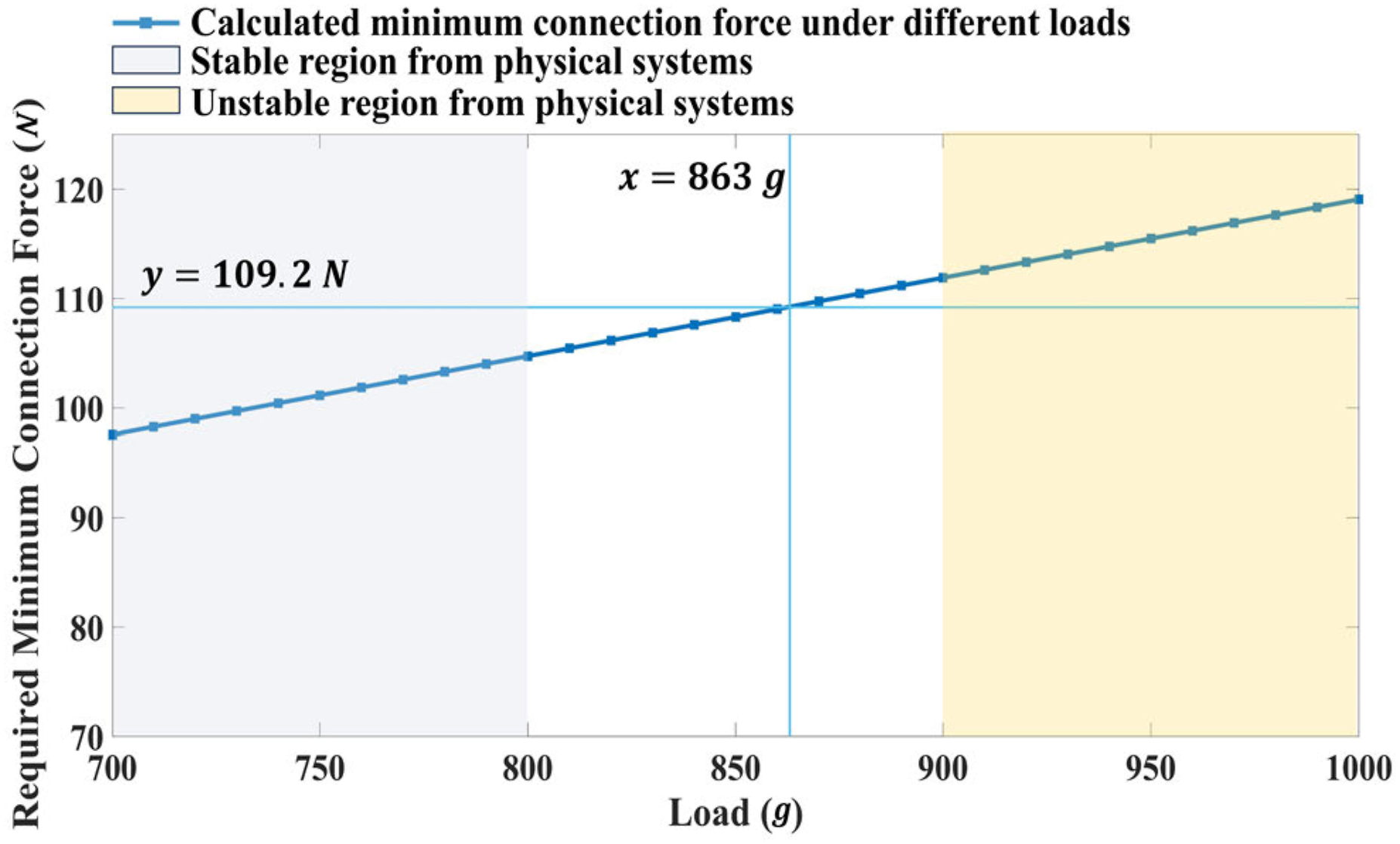

The impacts of unmodeled factors and input errors are varied for different configurations. The Configuration#1-5 have proved that the prediction derivation caused by the input is small enough to realize self-reconfiguration stability prediction. The load experiment further quantified the scale of this value.

6.4. Performance analysis

The quasi-static stability detection algorithm is anticipated to be executed on the module, with its invocation frequency being comparable to that of the obstacle avoidance algorithm. In previous research, taking into account the small deformations of the system, FE-based method are often utilized. A general stiffness model is proposed in Rimon et al. (2008) and the non-linear equation solver was used. The computation complexity of this method for n modules is about O(n^1.4) without collision detection. A linear-elastic FE model is used in Hołobut et al. (2020) and the computation cost is further decreased. However, the simplified model caused lower accuracy. The computation cost will further increase if friction and uneven planes are included in their model. We model the quasi-static stability problem of MSRR as a SOCP problem, which can be quickly solved using the interior point method. Frictional contact conditions and uneven terrains are also included in our model. We consider more factors, and the form of models is conducive to real-time computation.

For MSRR, the specific solving time depends on the system’s configuration, and the number of modules and contacts. We used FreeSN to randomly construct configurations with different number of modules. The proposed method was used to compute the minimum connection force. As shown in Figure 10, the average solution time of the algorithm linearly increases with the increase in the number of modules. The computation complexity of our method is about O(n + m), where n is the number of modules and m is the number of contacts. The proposed method greatly reduces the impact of the number of modules and is promising to be used in the real system to realize online planning.

Figure 10.

The average computation time of our proposed method for configurations with different number of modules.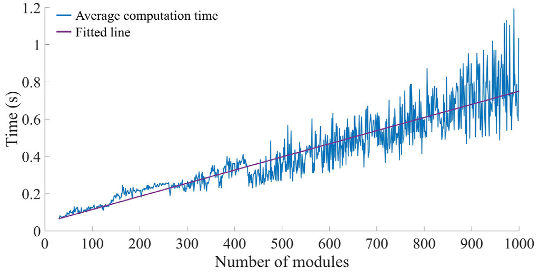

7. Conclusion

MSRR can form different configurations to perform tasks. They have strong task versatility, functionality, and self-repair ability. However, the mechanical connection stability between modules restricts their applications. In this paper, we model the mechanical stability problem as a SOCP problem. By minimizing the characteristic connection strength, we can obtain the critical stable state and potential broken connection points. By comparing the required minimum connection wrench with the physical connector constraints, we can detect this configuration’s stability under given external wrenches, including internal stability and whole-body stability. We also demonstrate two methods to determine the weight of the characteristic connection strength, for mechanical connection and magnetic connection respectively. However, obviously, the guaranteed stability does not exist. A system will be unstable as long as the external disturbances are strong enough. Therefore, a stability margin to evaluate the system’s anti-disturbance ability is important. Previous research has extensively discussed the whole-body stability margin (Bretl and Lall, 2008). Those research can directly be used for an MSRR system. In this paper, we propose the internal stability margin to evaluate the internal connection, which can be set as the indicator to realize robust reconfiguration and joint motion process.

We applied our method to the FreeSN system and did a series of simulation and physical experiments to test the accuracy and usability of this method, including two simulation analysis, one motion range experiment, five configuration experiments, one load experiment, and one time complexity experiment. The two simulation configurations show the effectiveness and applications of our method. The motion range experiment demonstrates that the point contact assumption and Lorentz cone are sufficient to model the connection coupling relationship of FreeSN. Configuration experiments show the proposed method can successfully predict the stability state of the system and can accurately point out the potential broken connection points. The load experiment further confirms the high prediction accuracy. Finally, we show that the solving time of the optimization problem increases linearly with the increase in the number of modules and contacts. In general, the model proposed in this paper is lightweight and can be solved quickly. We have reduced the impact of the number of modules to the greatest extent while algorithms can also provide accurate prediction results.

In the future, this detection method can be further improved by considering the influence of dynamic factors in MSRR.

Supplemental Material

Footnotes

Declaration of conflicting interests

The author(s) declared no potential conflicts of interest with respect to the research, authorship, and/or publication of this article.

Funding

The author(s) disclosed receipt of the following financial support for the research, authorship, and/or publication of this article: This work was supported by the Basic and Applied Basic Research Foundation of Guangdong Province (2023B1515020089), National Natural Science Foundation of China (62073274) and Shenzhen Institute of Artificial Intelligence and Robotics for Society (AC01202101103).

ORCID iDs

Di Wu

Guanqi Liang

Yuxiao Tu

Lijun Zong

Tin Lun Lam

Supplemental Material

Supplemental material for this article is available online.

References

Alberto

Avinash

Sergio

, et al. (2017) Current trends in reconfigurable modular robots design. International Journal of Advanced Robotic Systems 14(3): 1–21.

Bouyarmane

Caron

Escande

, et al. (2019) Multi-contact Motion Planning and Control. In: Goswami

Vadakkepat

(eds). Humanoid Robotics: A Reference. Dordrecht: Springer. doi: 10.1007/978-94-007-6046-2_32.

Boyd

Wegbreit

(2007) Fast computation of optimal contact forces. IEEE Transactions on Robotics 23(6): 1117–1132.

Bretl

Lall

(2008) Testing static equilibrium for legged robots. IEEE Transactions on Robotics 24(4): 794–807.

Butler

Rus

(2003) Distributed planning and control for modular robots with unit-compressible modules. The International Journal of Robotics Research 22(9): 699–715.

Chennareddy

SSR

Agrawal

Karuppiah

(2017) Modular self-reconfigurable robotic systems: a survey on hardware architectures. Journal of Robotics 2017: 1–19.

Del Prete

Tonneau

Mansard

(2016) Fast algorithms to test robust static equilibrium for legged robots In: 2016 IEEE International Conference on Robotics and Automation (ICRA), Stockholm Sweden, 16-21 May 2016, 1601–1607.

Dokuyucu

Özmen

(2023) Achievements and future directions in self-reconfigurable modular robotic systems. Journal of Field Robotics 40(3): 701–746.

García de Jalón

Gutiérrez-López

(2013) Multibody dynamics with redundant constraints and singular mass matrix: existence, uniqueness, and determination of solutions for accelerations and constraint forces. Multibody System Dynamics 30(3): 311–341.

10.

Grand

Benamar

Plumet

, et al. (2004) Stability and traction optimization of a reconfigurable wheel-legged robot. The International Journal of Robotics Research 23(10-11): 1041–1058.

11.

Hamlin

Sanderson

(1996) Tetrobot modular robotics: prototype and experiments In: 1996 IEEE/RSJ International Conference on Intelligent Robots and Systems (IROS),

Osaka Japan, 8

Nov. 1996, (Vol. 2)390–395.

12.

Hiller

Lipson

(2012) Automatic design and manufacture of soft robots. IEEE Transactions on Robotics 28(2): 457–466.

13.

Hiller

Lipson

(2014) Dynamic simulation of soft multimaterial 3d-printed objects. Soft Robotics 1(1): 88–101.

14.

Hołobut

Bordas

SPA

Lengiewicz

(2020) Autonomous model-based assessment of mechanical failures of reconfigurable modular robots with a conjugate gradient solver. In: 2020 IEEE/RSJ International Conference on Intelligent Robots and Systems (IROS),

Las

Vegas USA, 25 Oct – 25 Nov 2020, 11696–11702.

15.

Hołobut

Lengiewicz

(2017) Distributed computation of forces in modular-robotic ensembles as part of reconfiguration planning. In: 2017 IEEE International Conference on Robotics and Automation (ICRA), Singapore, 29 May-3 June 2017, 2103–2109.

16.

Jing

Tosun

Yim

, et al. (2018) Accomplishing high-level tasks with modular robots. Autonomous Robots 42: 1337–1354.

17.

Wei

Jin

, et al. (2024) Investigating stability outcomes across diverse gait patterns in quadruped robots: a comparative analysis. IEEE Robotics and Automation Letters 9(1): 795–802.

18.

Khatib

Jorda

Park

, et al. (2022) Constraint-consistent task-oriented whole-body robot formulation: task, posture, constraints, multiple contacts, and balance. The International Journal of Robotics Research 41(13-14): 1079–1098.

19.

Liang

Luo

, et al (2020) Freebot: a freeform modular self-reconfigurable robot with arbitrary connection point - design and implementation. In: 2020 IEEE/RSJ International Conference on Intelligent Robots and Systems (IROS),

Las

Vegas USA, 25 Oct - 25 Nov 2020, 6506–6513.

20.

Liang

, et al. (2024) Decoding modular reconfigurable robots: A survey on mechanisms and design. The International Journal of Robotics Research. doi: 10.1177/02783649241283847.

21.

Lin

Zhang

Shen

, et al (2019) Optimization based motion planning for multi-limbed vertical climbing robots. In: 2019 IEEE/RSJ International Conference on Intelligent Robots and Systems (IROS), Macau China, 3-8 Nov 2019, 1918–1925.

22.

Luo

Lam

(2022) Adaptive flow planning of modular spherical robot considering static gravity stability. IEEE Robotics and Automation Letters 7(2): 4228–4235.

23.

Luo

Lam

(2023) Auto-optimizing connection planning method for chain-type modular self-reconfiguration robots. IEEE Transactions on Robotics 39(2): 1353–1372.

24.

Marhefka

Orin

(1997) Gait planning for energy efficiency in walking machines. In: 1997 IEEE International Conference on Robotics and Automation (ICRA),

Albuquerque NM

USA, 25 April 1997, Vol. 1, 474–480.

25.

McGhee

(1967) Finite state control of quadruped locomotion. Simulation 9(3): 135–140.

26.

McGhee

Frank

(1968) On the stability properties of quadruped creeping gaits. Mathematical Biosciences 3: 331–351.

27.

Michael Grant and Stephen Boyd . Graph implementations for nonsmooth convex programs, Recent Advances in Learning and Control (a tribute to M. Vidyasagar). In: Blondel

Boyd

Kimura

(eds). Lecture Notes in Control and Information Sciences. Springer, 95–110.

28.

Nikolić

Borovac

Raković

(2018) Dynamic balance preservation and prevention of sliding for humanoid robots in the presence of multiple spatial contacts. Multibody System Dynamics 42: 197–218.

29.

Rimon

(2010) Analytic characterization of a class of three-contact frictional equilibrium postures in three-dimensional gravitational environments. The International Journal of Robotics Research 29(1): 3–22.

30.

Rimon

(2017) Characterization of frictional multi-legged equilibrium postures on uneven terrains. The International Journal of Robotics Research 36(1): 105–128.

31.

Várkonyi

(2021) Experimental verification of stability theory for a planar rigid body with two unilateral frictional contacts. IEEE Transactions on Robotics 37(5): 1634–1648.

32.

Pan

Liu

Gao

, et al. (2023) Joint search of optimal topology and trajectory for planar linkages. The International Journal of Robotics Research 42(4-5): 176–195.

33.

Pang

Trinkle

(2000) Stability characterizations of rigid body contact problems with coulomb friction. Journal of Applied Mathematics and Mechanics 80(10): 643–663.

34.

Park

Yim

, et al. (2019) Optimization-based nonimpact rolling locomotion of a variable geometry truss. IEEE Robotics and Automation Letters 4(2): 747–752.

35.

Piranda

Chodkiewicz

Hołobut

, et al. (2021) Distributed prediction of unsafe reconfiguration scenarios of modular robotic programmable matter. IEEE Transactions on Robotics 37(6): 2226–2233.

36.

Rimon

Mason

Burdick

, et al. (2008) A general stance stability test based on stratified morse theory with application to quasi-static locomotion planning. IEEE Transactions on Robotics 24(3): 626–641.

37.

Sastra

Chitta

Yim

(2009) Dynamic rolling for a modular loop robot. The International Journal of Robotics Research 28(6): 758–773.

38.

Seo

Paik

Yim

(2019) Modular reconfigurable robotics. Annual Review of Control, Robotics, and Autonomous Systems 2(1): 63–88.

39.

Shen

Krivokon

Chiu

, et al. (2006) Multimode locomotion via superbot reconfigurable robots. Autonomous Robots 20: 165–177.

40.

Suh

Homans

Yim

(2002) Telecubes: mechanical design of a module for self-reconfigurable robotics. 2002 International Conference on Robotics and Automation (ICRA) 4: 4095–4101.

41.

Lam

(2023) Configuration identification for a freeform modular self-reconfigurable robot - freesn. IEEE Transactions on Robotics 39: 4636–4652.

42.

Liang

Lam

(2022) Freesn: a freeform strut-node structured modular self-reconfigurable robot - design and implementation. In: 2022 International Conference on Robotics and Automation (ICRA), Philadelphia PA USA, 23 - 27 May 2022, 4239–4245.

43.

Varshavskaya

Kaelbling

Rus

(2008) Automated design of adaptive controllers for modular robots using reinforcement learning. The International Journal of Robotics Research 27(3-4): 505–526.

44.

White

Revzen

Thorne

, et al. (2011) A general stiffness model for programmable matter and modular robotic structures. Robotica 29(1): 103–121.

45.

Wojtyra

(2017) Modeling of static friction in closed-loop kinematic chains—uniqueness and parametric sensitivity problems. Multibody System Dynamics 39: 337–361.

46.

Yao

Belke

Cui

, et al. (2019) A reconfiguration strategy for modular robots using origami folding. The International Journal of Robotics Research 38(1): 73–89.

47.

Yim

Duff

Zhang

(2001) Closed-chain motion with large mechanical advantage. In: 2001 IEEE/RSJ International Conference on Intelligent Robots and Systems (IROS), Maui HI USA, 29 Oct - 3 Nov 2001, Vol. 1, 318–323.

48.

Yim

Shen

Salemi

, et al. (2007) Modular self-reconfigurable robot systems [grand challenges of robotics]. IEEE Robotics and Automation Magazine 14(1): 43–52.

49.

Yoshida

Murata

Kamimura

, et al. (2002) A self-reconfigurable modular robot: reconfiguration planning and experiments. The International Journal of Robotics Research 21(10-11): 903–915.

50.

Zhang

Fasse

(2000) Spatial compliance modeling using a quaternion-based potential function method. Multibody System Dynamics 4: 75–101.

51.

Zhao

Lam

(2022) Snailbot: a continuously dockable modular self-reconfigurable robot using rocker-bogie suspension. In: 2022 International Conference on Robotics and Automation (ICRA), Philadelphia PA USA, 23 - 27 May 2022, 4261–4267.

52.

Zong

Liang

Lam

(2023) Kinematics modeling and control of spherical rolling contact joint and manipulator. IEEE Transactions on Robotics 39(1): 738–754.

Supplementary Material

Please find the following supplemental material available below.

For Open Access articles published under a Creative Commons License, all supplemental material carries the same license as the article it is associated with.

For non-Open Access articles published, all supplemental material carries a non-exclusive license, and permission requests for re-use of supplemental material or any part of supplemental material shall be sent directly to the copyright owner as specified in the copyright notice associated with the article.

0.00 MB