Recursive model-agnostic inverse dynamics of serial soft-rigid robots

Abstract

Robotics is shifting from rigid, articulated systems to more sophisticated and heterogeneous mechanical structures. Soft robots, for example, have continuously deformable elements capable of large deformations. The flourishing of control techniques developed for this class of systems is fueling the need of efficient procedures for evaluating their inverse dynamics (ID), which is challenging due to the complex and mixed nature of these systems. As of today, no single ID algorithm can describe the behavior of generic (combinations of) models of soft robots. We address this challenge for generic series-like interconnections of possibly soft structures that may require heterogeneous modeling techniques. Our proposed algorithm requires as input a purely geometric description (forward-kinematics-like) of the mapping from configuration space to deformation space. With this information only, the complete equations of motion can be given an exact recursive structure which is essentially independent from (or “agnostic” to) the underlying reduced-order kinematics. We achieve this by exploiting Kane’s method to manipulate the equations of motion, showing then their recursive structure. The resulting ID algorithms have optimal computational complexity within the proposed setting, that is, linear in the number of distinct modules. Further, a variation of the algorithm is introduced that can evaluate the generalized mass matrix without increasing computation costs. We showcase the method applicability to robot models involving a mixture of rigid and soft elements, described via possibly heterogeneous reduced order models (ROMs), such as Volumetric FEM, Cosserat strain-based, and volume-preserving deformation primitives. None of these systems can be handled using existing ID techniques.

Keywords

Modeling and control of soft robots serial soft-rigid robots inverse dynamics recursive Kane’s equations theoretical foundations soft robotics

1. Introduction

In recent years, robotic systems have undergone a remarkable transformation, evolving from assemblies of rigid links and joints to articulated mechanical architectures built from complex modules. These include serial interconnections of parallel mechanisms (Lee et al., 2009), flexible link and joint manipulators (De Luca and Book, 2016), robots made of meta-materials (Bevilacqua et al., 2022; Hu et al., 2020), continuum and soft arms (Hoeijmakers et al., 2022; Liu et al., 2023a; Rus and Tolley, 2015; Russo et al., 2023; Yin et al., 2021), bio-hybrid robots (Lin et al., 2022; Sun et al., 2020; Wang et al., 2021), and rigid robots manipulating deformable objects (Tiburzio et al., 2024; Zhu et al., 2022). In this work, we specifically focus on one such class of systems: soft robots. Unlike rigid robots, where motion originates from the joints, soft robots leverage their compliant and highly deformable bodies to move (Della Santina et al., 2020a).

However, the advantages of the soft body come with substantial challenges in modeling and control (Della Santina et al., 2023) due to the infinite dimensionality of the dynamics. The control of infinite-dimensional mechanical systems is still an emerging field of research (Chang et al., 2023; Han et al., 2021; Zheng and Lin, 2022). Reduced order models (ROMs) have been thoroughly investigated as an alternative to PDE descriptions (Boyer et al., 2020; Dinev et al., 2018; Grazioso et al., 2019; Qin et al., 2024; Renda et al., 2018). These range from volumetric FEM (Dubied et al., 2022; Ferrentino et al., 2023; Ménager et al., 2023), possibly combined with model order reduction techniques, to strain-based Cosserat descriptions (Boyer et al., 2020; Caasenbrood et al., 2023; Renda et al., 2020), to other techniques specifically tailored to soft robots–like quasi-rigid models (Sfakiotakis et al., 2014) or volume-preserving primitives (Xu and Chirikjian, 2023). Despite the vast heterogeneity, all these techniques follow the principles of Lagrangian mechanics and are described by ordinary differential equations of the form

M (q) \ddot{q} + c (q, \dot{q}) + g (q) + s (q, \dot{q}) = ν (q, u),

(1)

where symbols are defined in Table 1. The Inverse Dynamics (ID) problem refers to the challenge of computing the left-hand side of (1). The ID problem plays a pivotal role in various applications that are crucial for the advancement of autonomous and intelligent robotic systems, including real-time control (Boyer et al., 2020; Buondonno and De Luca, 2016; Liu et al., 2023b), system identification (Gaz et al., 2019), trajectory generation (Longhini et al., 2023) and optimization (Ferrolho et al., 2021; Saunders et al., 2010), and mechanical design (Chen and Wang, 2020; Pinskier and Howard, 2022). For example, in case of full actuation, it is a common control approach to feedback linearize the system via direct application of the ID law:

ν = M (q) α + c (q, \dot{q}) + g (q) + s (q, \dot{q})

, where α is a control acceleration. In all these contexts, the ID must be executed in real-time or faster. Thus, computational efficiency becomes essential, especially when the dynamics has many DoFs.¹ In this context, recursive formulations of the ID have been imposed themselves as a way of solving the ID problem with minimal computational time (Featherstone, 2014). Indeed, recursive ID algorithms scale linearly with the number of bodies, whereas non-recursive algorithms scale quadratically. As a result, the former require less resources and offer faster computation times, particularly in systems with many bodies.

Table 1.

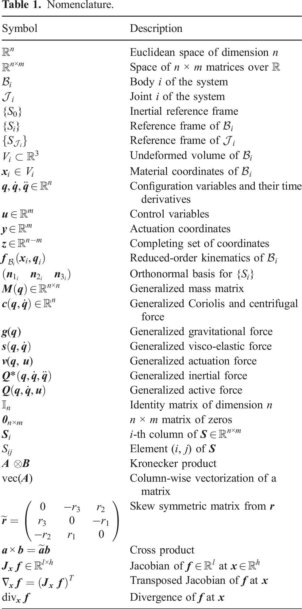
Nomenclature.

Symbol	Description
$R^{n}$	Euclidean space of dimension n
$R^{n \times m}$	Space of n × m matrices over $R$
$B_{i}$	Body i of the system
$J_{i}$	Joint i of the system
{S₀}	Inertial reference frame
{S_i}	Reference frame of $B_{i}$
${S_{J_{i}}}$	Reference frame of $J_{i}$
$V_{i} \subset R^{3}$	Undeformed volume of $B_{i}$
x _i ∈ V_i	Material coordinates of $B_{i}$
$q, \dot{q}, \ddot{q} \in R^{n}$	Configuration variables and their time derivatives
$u \in R^{m}$	Control variables
$y \in R^{m}$	Actuation coordinates
$z \in R^{n - m}$	Completing set of coordinates
$f_{B_{i}} (x_{i}, q_{i})$	Reduced-order kinematics of $B_{i}$
$(n_{1_{i}} n_{2_{i}} n_{3_{i}})$	Orthonormal basis for {S_i}
$M (q) \in R^{n \times n}$	Generalized mass matrix
$c (q, \dot{q}) \in R^{n}$	Generalized Coriolis and centrifugal force
g ( q )	Generalized gravitational force
$s (q, \dot{q})$	Generalized visco-elastic force
ν ( q , u )	Generalized actuation force
$Q^{*} (q, \dot{q}, \ddot{q})$	Generalized inertial force
$Q (q, \dot{q}, u)$	Generalized active force
$I_{n}$	Identity matrix of dimension n
0 _n×m	n × m matrix of zeros
S _i	i-th column of $S \in R^{n \times m}$
S _ij	Element (i, j) of S
A ⊗ B	Kronecker product
vec( A )	Column-wise vectorization of a matrix
$\tilde{r} = (\begin{matrix} 0 & - r_{3} & r_{2} \\ r_{3} & 0 & - r_{1} \\ - r_{2} & r_{1} & 0 \end{matrix})$	Skew symmetric matrix from r
$a \times b = \tilde{a} b$	Cross product
$J_{x} f \in ℝ^{l \times h}$	Jacobian of $f \in R^{l}$ at $x \in R^{h}$
$\nabla_{x} f = {(J_{x} f)}^{T}$	Transposed Jacobian of f at x
div_x f	Divergence of f at x

Substantial research has been done on recursive ID for non-conventional robotic structures, as discussed in Section 1.1, with some focused attention already being devoted to continuum soft robots (Boyer et al., 2020; Godage et al., 2019; Jensen et al., 2022). However, all existing recursive methods have the disadvantage of being specifically tailored to a single ROM technique, thus severely constraining the range of systems that can be dealt with.

This work proposes a more holistic recursive formulation of soft-rigid systems. Being agnostic to the underlying reduced order kinematic modeling technique, it can deal with a vast range of systems and is readily applicable to novel kinds of structures or models, including existing methods as sub-cases. A key enabling idea of our approach is to treat kinematics as an input to the procedure rather than a predefined information. In particular, the robot is seen as an assembly of kinematic modules (joints or deformable bodies) whose relative motion is parameterized by a generic kinematics-like function of material and configuration variables. Beside assuming that the kinematics belongs to a finite-dimensional space, the only hypothesis is that the contact area between two adjacent modules does not deform. The proposed derivations build on the Kane method (Banerjee, 2022; Kane and Levinson, 1983), which is an equivalent form of the virtual work principle. For the first time, we demonstrate that the Kane equations can be manipulated to obtain a recursive formulation of the dynamics, independent of the soft body kinematics. This result has two implications. First, both existing and new kinematic models can be seamlessly integrated into our framework. Second, it enables the efficient computation of the ID. The resulting equations of motion (EoM) can be viewed as a recursive form of the Euler–Lagrange (EL) equations and a generalization to the seminal results of Hollerbach (1980) and Book (1984). These works derived a recursive EL equations with linear complexity for serial rigid (Hollerbach, 1980) and flexible link robots (Book, 1984). Analogous to the Newton–Euler approach for rigid systems, our proposed method has a cost that is linear in the number of bodies or, equivalently, in the number of DoFs. However, as we shall see, treating the kinematics as a black-box function limits recursivity to the system bodies, preventing its extension to the material domain—unlike ID algorithms designed for specific kinematic models.

The main contributions of the paper are summarized below.

(1) We derive a model-agnostic recursive formulation of the EoM for generic (i.e., agnostic to discretization technique) serial soft-rigid robots whose bodies are rigidly connected to the joints.

(2) By exploiting this recursive representation of the dynamics, we introduce two novel algorithms for computing the generalized active and actuation forces. In both cases, we prove that the computational complexity grows linearly with the number of DoFs.

(3) We demonstrate how the algorithms solving the ID problem can be minimally modified to evaluate the mass matrix without affecting computational complexity. Additionally, we propose embedding such computation within the ID algorithms, as it provides greater flexibility for control purposes.

The findings are supported by numerical results on multiple robotic systems—which cannot be handled using current recursive methods. We present for the first time a dynamic simulation with the control of a trimmed helicoid robot using the locally volume preserving (LVP) primitives method (Xu and Chirikjian, 2023) for 3D continua. In a second simulation, we consider a hybrid arm consisting of a rigid manipulator, a slender soft body modeled using the geometric variable strain (GVS) approach (Boyer et al., 2020), and a soft gripper with LVP kinematics. We show then how the proposed recursive equations scale with the number of bodies compared to the EL approach, which is the only framework that currently can describe the class of robotic systems considered in this paper.

1.1. State of the art on ID problem

Numerous studies have explored the computation of the ID problem for slender flexible link robots, that is, under the small deformations assumption, using different approaches. These include the EL method (Book, 1984; Chen, 2001; Zhang, 2009; My et al., 2019), the generalized Newton–Euler (NE) equations (Boyer and Khalil, 1998; Khalil et al., 2017; Shabana, 1990), the Gibb–Appell equations (Korayem et al., 2014), and the Kane equations (Amirouche and Xie, 1993; Banerjee and Dickens, 1990; Singh et al., 1985). All the mentioned works share three main assumptions: (i) small deflections, (ii) slender bodies, and (iii) the possibility to approximate the deformable motion, that is, changes in shape and size, as a linear function of the configuration variables—a set of independent parameters that uniquely define the body relative position. Unfortunately, assumptions (i) and (iii) are seldom verified by ROMs of soft robotic systems. Consequently, new ID algorithms have been developed to relax the above assumptions to some extent.

Under a rigid-body discretization and the piecewise constant curvature kinematic model, Rone and Ben-Tzvi (2013) present a procedure based on the Kane method to evaluate the ID of slender continuum manipulators. Later, under the same kinematic assumptions, Godage et al. (2019) follow a Lagrangian approach to compute the dynamic matrices with a O(n²) cost, where n is the total number of DoFs. Although not explicitly stated, this procedure can also be used to evaluate the ID. In Jensen et al. (2022), the authors apply the recursive Newton–Euler algorithm for rigid body systems to a lumped mass model of a six-DoFs slender soft arm with piecewise constant curvature. Under the Cosserat rod hypothesis, Renda et al. (2018) propose an ID procedure for robots with piecewise constant strain (PCS). By leveraging the rigidity of the robot cross sections, the authors derive a recursive ID algorithm that generalizes the Newton–Euler procedure for rigid arms. This algorithm has computational complexity linear in the number of bodies, making it optimal. The method was extended in Renda and Seneviratne (2018) to consider hybrid systems consisting of PCS soft and rigid bodies. Later, Boyer et al. (2020) relaxed the PCS hypothesis in favor of a modal Ritz reduction of the strain. Recently, Mathew et al. (2024) introduced a state- and time-dependent basis of the strain. These recursive methods are limited to bodies satisfying the Cosserat rod assumption, that is, thin bodies (hypothesis (ii)) with rigid cross sections, and, consequently, are inapplicable to kinematic models of non-slender soft robotic systems (Sharp et al., 2023; Xu and Chirikjian, 2023). Nonetheless, it is important to note that ID algorithms for discrete Cosserat rods enable a more efficient computation compared to our method. Specifically, the degree of recursivity applies not only between the bodies of the system—as in our approach—but also within the soft material domain. This advantage arises because the kinematics of Cosserat rods can be leveraged to obtain recursivity also within the soft material domain and, consequently, improve the speed of the algorithm.

Finally, Sadati et al. (2021) introduced the TMT method for soft bodies. This approach enables the derivation of (1) in vector form, reducing the number of required steps compared to the EL method. While it facilitates a more efficient implementation of the dynamics, it still maintains the quadratic computational cost of a non-recursive formulation. Moreover, although the TMT method has been successfully applied to compute the ID of various reduced-order kinematic models for soft robots, its extension to 2D and 3D geometries assumes that these bodies can be modeled as wire meshes, where edges correspond to 1D Euler–Bernoulli beams and connections are point masses. Consequently, its applicability to the generic kinematic models considered in this work remains unexplored.

To summarize, the main benefits of our approach are as follows:

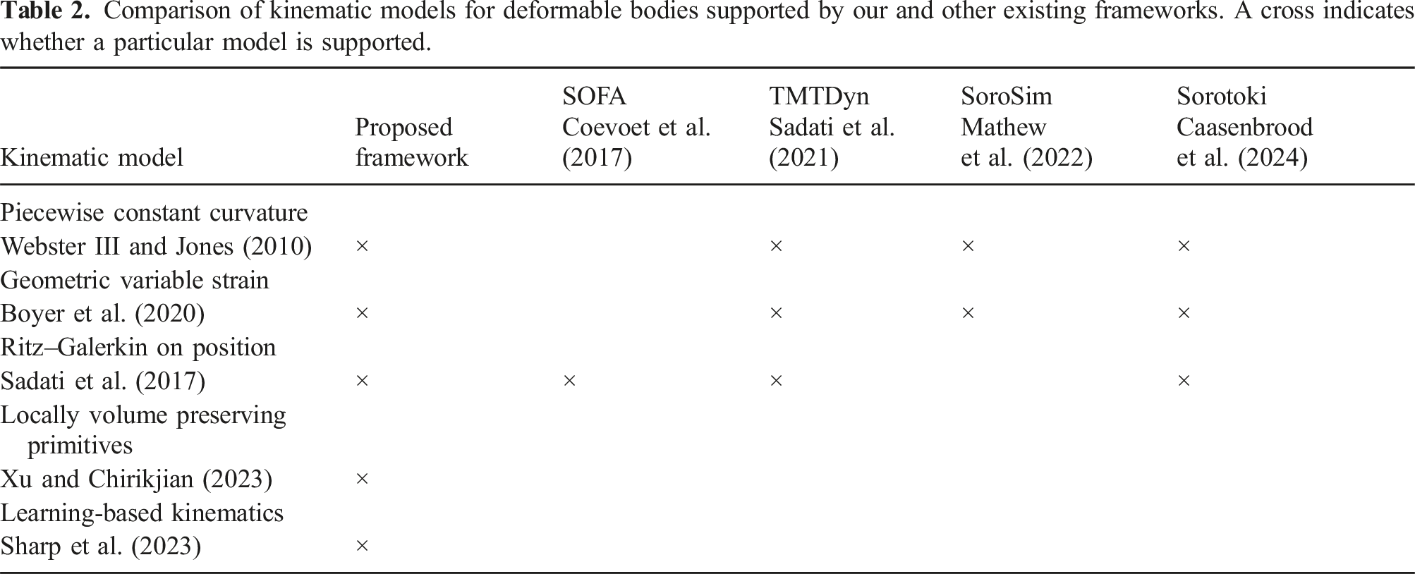
• It is possible to evaluate the ID for robots with arbitrarily deformable bodies, such as rigid arms with soft grippers and non-slender soft manipulators. Table 2 provides a non-exhaustive list of models supported by our framework compared to other existing solutions.

• In view of the recursive formulation, the computation of the ID scales linearly with number of bodies.

• Since the method is agnostic to the kinematics, new models can be easily conceptualized and applied in control tasks.

On the other hand, the following limitations exist:

• It is not possible to exploit recursivity within the soft material domain. As a result, for certain subclasses of kinematic models, more efficient algorithms may be available.

• The derivations rely on the assumption that the soft bodies kinematics is purely geometrical.

• The introduction of an abstraction layer on the kinematics could make the model more difficult to understand and interpret.

Table 2.

Comparison of kinematic models for deformable bodies supported by our and other existing frameworks. A cross indicates whether a particular model is supported.

Kinematic model	Proposed framework	SOFACoevoet et al. (2017)	TMTDynSadati et al. (2021)	SoroSimMathew et al. (2022)	SorotokiCaasenbrood et al. (2024)
Piecewise constant curvature
Webster III and Jones (2010)	×		×	×	×
Geometric variable strain
Boyer et al. (2020)	×		×	×	×
Ritz–Galerkin on position
Sadati et al. (2017)	×	×	×		×
Locally volume preserving primitives
Xu and Chirikjian (2023)	×
Learning-based kinematics
Sharp et al. (2023)	×

1.2. Notation

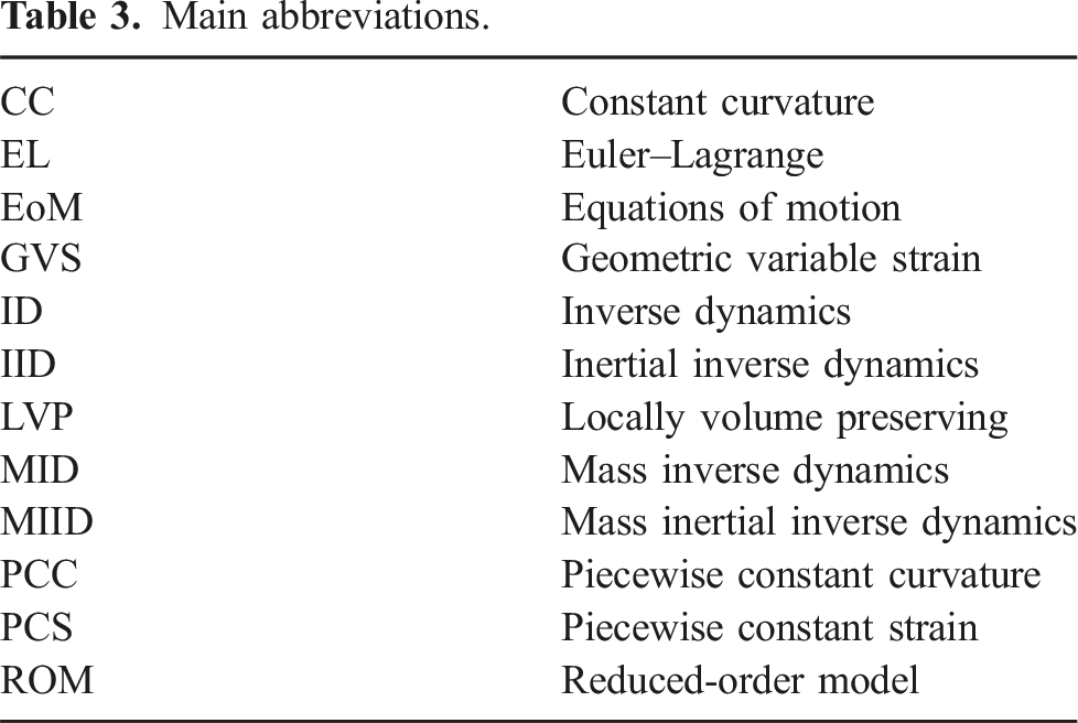
We denote vectors and matrices with bold letters. Arguments of the functions are omitted when clear from the context. Beside the notation adopted in the paper (see Table 1), Table 3 summarizes also the main abbreviations used in the text.

Table 3.

Main abbreviations.

CC	Constant curvature
EL	Euler–Lagrange
EoM	Equations of motion
GVS	Geometric variable strain
ID	Inverse dynamics
IID	Inertial inverse dynamics
LVP	Locally volume preserving
MID	Mass inverse dynamics
MIID	Mass inertial inverse dynamics
PCC	Piecewise constant curvature
PCS	Piecewise constant strain
ROM	Reduced-order model

1.3. Code

We also provide in a GitHub repository an expandable object-oriented MATLAB library with full C/C++ code generation functionality implementing all the algorithms presented in the following.

1.4. Supplementary material

In this paper, we show numerical results on recently introduced kinematic models of soft robots. However, the proposed strategy can be seamlessly applied to more conventional robots, such as Cosserat rods. The interested reader can find supplementary material detailing the application of the method to other systems at the link Supplementary Material.

1.5. Structure of the paper

The rest of the paper is organized as follows. In Section 2, we formally introduce the goal of the paper. In Section 3, we discuss the proposed kinematics-as-an-input setting and establish the configuration space that characterizes the considered class of systems. Herein, we introduce the direct and the first- and second-order differential kinematics. Section 4 presents the Kane equations for the system. Their recursive form is obtained in Section 5, offering immediate utility in assessing generalized active forces with cost linear in the number of bodies. We also demonstrate how this recursive structure can be exploited to evaluate the mass matrix without affecting computational complexity. In Section 6, we expand the active forces to derive a recursive procedure for evaluating only the actuation forces in the ID problem. Section 7 presents simulations results, and Section 8 draws the main conclusions of the paper and includes future work.

2. Problem statement

In this section, we define the ID problem for the class of robots under consideration and introduce the two hypotheses under which it is addressed: (i) the kinematics of deformable bodies can be described geometrically using a finite number of configuration variables and (ii) the bodies are connected through rigid joints.

Consider a holonomically constrained² serial chain with fixed base constituted by N moving bodies $B_{i}$ , each connected to its predecessor by a joint $J_{i}$ , for i = 1, …, N. From now on, if not explicitly stated, the subscript (⋅)_i refers to a quantity of body or joint i.

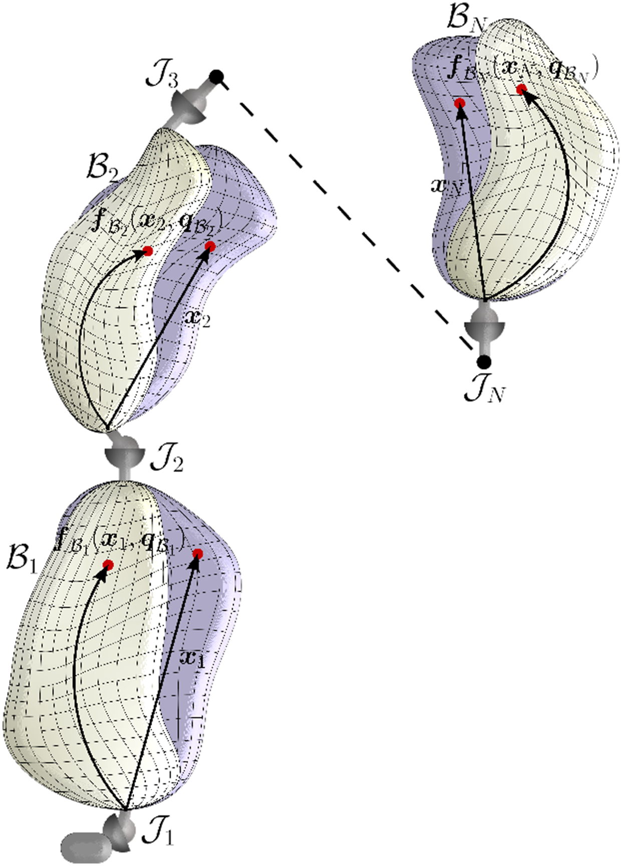
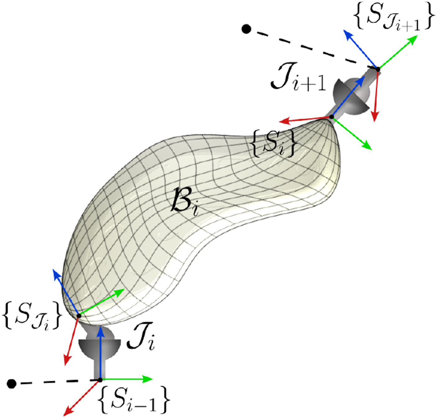
Assume that the following conditions hold, as illustrated in Figure 1.

Assumption 1

The kinematics of each body $B_{i}$ belongs to a finite-dimensional configuration space.

Mathematically, Assumption 1 requires that the position $p_{B_{i}} \in R^{3}$ of each body point relative to the distal end of its joint takes the form

p_{B_{i}} = f_{B_{i}} (x_{i}, q_{B_{i}}),

(2)

where

x_{i} \in V_{i} \subset R^{3}

collects the Cartesian material coordinates of

B_{i}

in the reference (stress-free) configuration V_i,

q_{B_{i}} \in R^{n_{B_{i}}}

parameterizes the body motions, and

f_{B_{i}}

is a generic function, possibly highly nonlinear in both arguments. The previous equation implicitly requires that the kinematics can be described purely geometrically. In other words, the dependence of

p_{B_{i}}

on external forces, such as those of actuation u , is not modeled explicitly. Instead, this dependence arises through the dynamic influence of u on

q_{B_{i}}

, as expressed in (1). This simplification, which is widely adopted in the reduced-order modeling of soft robots, Boyer et al., 2020; Caasenbrood et al., 2024; Della Santina et al., 2020b; Sadati et al., 2021; Xu and Chirikjian, 2023, can be motivated as follows. The instantaneous effects of u on the kinematics can be reasonably captured by introducing additional configuration variables, which are then influenced by u through the EoM. Examples of this approach can be found in Simulation 2 of the paper and Simulation 4 in the supplementary material.

Assumption 2

For each body, the contact areas at the joints do not deform.

This assumption reasonably holds for the majority of soft robotic systems since a joint typically introduces some degree of rigidity at the contact areas. As we shall see, Assumption 2 is not required from the perspective of the dynamics equations and does not effect the recursion, but it is necessary for describing the robot kinematics in presence of non-fixed joints. As a matter of fact, when the bodies are linked through fixed joints, it can be removed. Relaxation of the above assumption will be considered in one of the simulations.

Remark 1

We do not assume any specific structure for (2) and consider it an input to the ID procedure, similar to the approach of Featherstone (2014) for rigid robots. This allows us to decouple the kinematic assumption typically made to solve the ID problem for specific sub-classes of soft robots from the algorithm itself. For the purposes of this paper, the reader should consider $f_{B_{i}}$ as a black-box function, which could be obtained in various ways (Sharp et al., 2023; Xu and Chirikjian, 2023). This structure also encompasses popular kinematic functions used in soft robot modeling (Sadati et al., 2020), such as reduced-order FEM (Ménager et al., 2023) and discrete Cosserat models (Della Santina et al., 2023; Renda et al., 2020).

Assumption 1 implies that the robot dynamics follows the principles of Lagrangian mechanics, thus taking the form of (1) and leading to the following problems.

Problem 1

Inertial Inverse Dynamics Problem. Under Assumption 1 and 2, find an algorithm $I I D (q, \dot{q}, \ddot{q})$ with O(N) complexity such that

I I D (q, \dot{q}, \ddot{q}) = M (q) \ddot{q} + c (q, \dot{q}) .

Problem 2

Inverse Dynamics Problem. Under the same hypotheses of Problem 1, find an algorithm $I D (q, \dot{q}, \ddot{q})$ with O(N) complexity such that

I D (q, \dot{q}, \ddot{q}) = M (q) \ddot{q} + c (q, \dot{q}) + g (q) + s (q, \dot{q}) .

It is worth remarking that we consider the output of the ID as the generalized actuation force ν ( q , u ), rather than the control variables u , as done for rigid fully-actuated robots. This choice is motivated by two considerations. First, the expression of ν depends on the type of actuation and how it is modeled. Consequently, deriving a general method to compute u from ν is not straightforward. As shown in Section 7, when ν ( q , u ) = A ( q ) u and A ( q ) satisfies certain integrability conditions (Pustina et al., 2024), a change of coordinates allows u to directly influence the dynamics, making it possible to compute u directly through the ID algorithm. However, this is a relatively specific case and does not universally apply. Second, the actuation forces commonly used in soft robotics are often subject to constraints (Bruder et al., 2021; Tonkens et al., 2021). For example, a tendon can only generate a pulling force, which must be taken into account when computing u from ν (Della Santina et al., 2019).

Another important aspect to discuss is the relationship between the inputs to the IID and ID procedures, namely q , $\dot{q}$ and $\ddot{q}$ , the generalized actuation force ν ( q , u ), and the control variables u . Even in finite-dimensional models of soft robotic systems, the number of control variables is typically less than the number of generalized coordinates, that is, m < n. This implies that u can only directly control the evolution of a subset of the configuration variables q or, in general, a vector of output variables y of dimension m (assuming all control inputs are independent). Consequently, n − m configuration variables do not evolve freely. As a result, if the ID algorithm in a given state $(q, \dot{q})$ is supplied with an arbitrary acceleration value $\ddot{q}$ , there is no guarantee that a command u exists such that (1) holds. In other words, at any given instant t, there may not exist a u such that $ν (q (t), u) = I D (q (t), \dot{q} (t), \ddot{q} (t))$ . This issue can potentially be resolved if there exists a set of generalized coordinates $θ = {(y^{T} z^{T})}^{T}$ such that $y \in R^{m}$ —referred to hereinafter as actuation coordinates—can be directly controlled through u , and $z \in R^{n - m}$ is the complement to y of coordinates not directly actuated by u . In this scenario, the unactuated coordinates z satisfy a set of second-order differential constraints that takes the form $\ddot{z} = - M_{z z}^{- 1} (M_{z y} \ddot{y} + c_{z} + g_{z} + s_{z}),$ with suitable sub-blocks of the dynamic terms in (1) rewritten in the θ coordinates. Thus, for any generic state $(y, z, \dot{y}, \dot{z})$ and arbitrary $\ddot{y}$ , selecting $\ddot{z}$ according to the previous equation ensures that the output ν ( θ , u ) of the ID algorithm can be achieved by an appropriate choice of u . The existence of such actuation coordinates in generic soft robotic systems remains an open question and has only been explored so far when the dynamics is linear in the input (Pustina et al., 2024).

Note also that in addition to the ID problem (Problem 2), we introduce another problem to be solved, namely the Inertial Inverse Dynamics (IID) problem (Problem 1), for three reasons. First, active forces on the robot may also differ from those considered in (1)—despite $g (q) + s (q, \dot{q})$ is the most common case, or some of them may be absent, such as when the robot is moving on a horizontal plane. This approach allows us to initially focus on computing the inertial forces in IID, and only later distinguish the actuation forces (the unknowns) from the active forces. Second, by addressing Problem 1, we can concentrate on the inertial terms alone, which are the most challenging to compute. Third, the Kane equations yield naturally a distinction between inertial and active forces, driving us naturally to consider Problem 1 as well. Although we differentiate between these two problems, their solutions will be developed almost in parallel.

Remark 2

Because we are considering robots with a serial topology, the ID problem cannot be solved in less than O(N) steps (Featherstone, 2014). Additionally, since the number of DoFs n is a multiple of the number of bodies N, in terms of computational complexity one has O(N) = O(n).

Toy Example. To facilitate the understanding of our algorithms, throughout the paper we present the computation of the main terms required by our procedures for a planar soft body modeled under the Constant Curvature (CC) assumption (Della Santina et al., 2020b). This body is connected to its predecessor via a fixed joint and has a cylindrical shape with unitary radius and length. We choose a CC body for three main reasons. First, the CC kinematics is a well-known and widely used model in soft robotics. Second, despite its relative simplicity, the CC model exhibits significant nonlinearities, making the solution of the ID problem non trivial, even when the system has only a few bodies. Finally, Simulation 3 is a natural continuation of this example.

For the ease of reading, the short notation c_x and s_x stands for cos(x) and sin(x), respectively. Moreover, to avoid unnecessary use of subscripts, in this example only, we use the notation $q_{B_{i}} = q$ .

For the CC model, the reduced-order kinematics ( 2 ) reads

p_{B_{i}} = (\begin{matrix} \frac{c_{q x_{3}} - 1}{q} + x_{1} c_{q x_{3}} \\ x_{2} \\ \frac{s_{q x_{3}} (q x_{1} + 1)}{q} \end{matrix}),

where x₁ and x₂ parametrize a circle of unitary radius, namely the robot cross section, and x₃ ∈ [0, 1], that is, x₃ represents the distance from the base.

3. Kinematics

As a preliminary step towards solving Problem 1, this section characterizes the forward kinematics for a robot whose bodies kinematics take the generic form (2). We also briefly introduce the first and second-order differential kinematics, which will be used later in the solution of the ID.

A complete description of the kinematics requires introducing two types of reference frames: a reference frame {S_i} at the pivot point between $B_{i}$ and $J_{i + 1}$ with the same orientation of their rigid contact area, and another one ${S_{J_{i}}}$ at the distal end of $J_{i}$ with the same orientation of the area between $J_{i}$ and $B_{i}$ , as illustrated in Figure 2. Note that other choices are possible, but still a pair of reference frames is needed for each body as explained below. An inertial reference frame {S₀} is also attached to the robot base, where the dynamics will be formulated.

The frame {S_i} is used in conjunction with ${S_{J_{i}}}$ to track the relative motion between adjacent bodies as a consequence of the joint presence. Indeed, the relative position and orientation between $J_{i}$ and $J_{i + 1}$ changes not only because of the joint motion but also because of $B_{i}$ deformability, thus requiring a reference frame ({S_i}) attached to $B_{i}$ as well. In other words, at the kinematic level only, $B_{i}$ can be seen as a distributed joint that requires as such its own reference frame. This is also the reason why Assumption 2 is taken. As we shall see, this hypothesis allows us to describe the orientation of {S_i} starting from $f_{B_{i}}$ . On the other hand, if the robot contains some bodies connected by fixed joints, one can adopt three possible strategies: (i) remove Assumption 2 for the bodies connected by fixed joints and describe the kinematics using only the pairs {S_i} and ${S_{J_{i}}}$ associated to bodies connected by non-fixed joints; (ii) retain Assumption 2 and introduce a single reference frame {S_i} for bodies connected by fixed joints; or (iii) maintain all reference frames and let ${S_{i}} = {S_{J_{i + 1}}}$ . In the following, to consider the more general case, that is, the case of a robot with moving joints, we adopt the third strategy. Note also that because of the same above reason, for the last body $B_{N}$ , one does not need in principle to introduce {S_N} but only ${S_{J_{N}}}$ . We now move to the computation of the homogeneous transformation matrices describing the relative motion between the above frames.

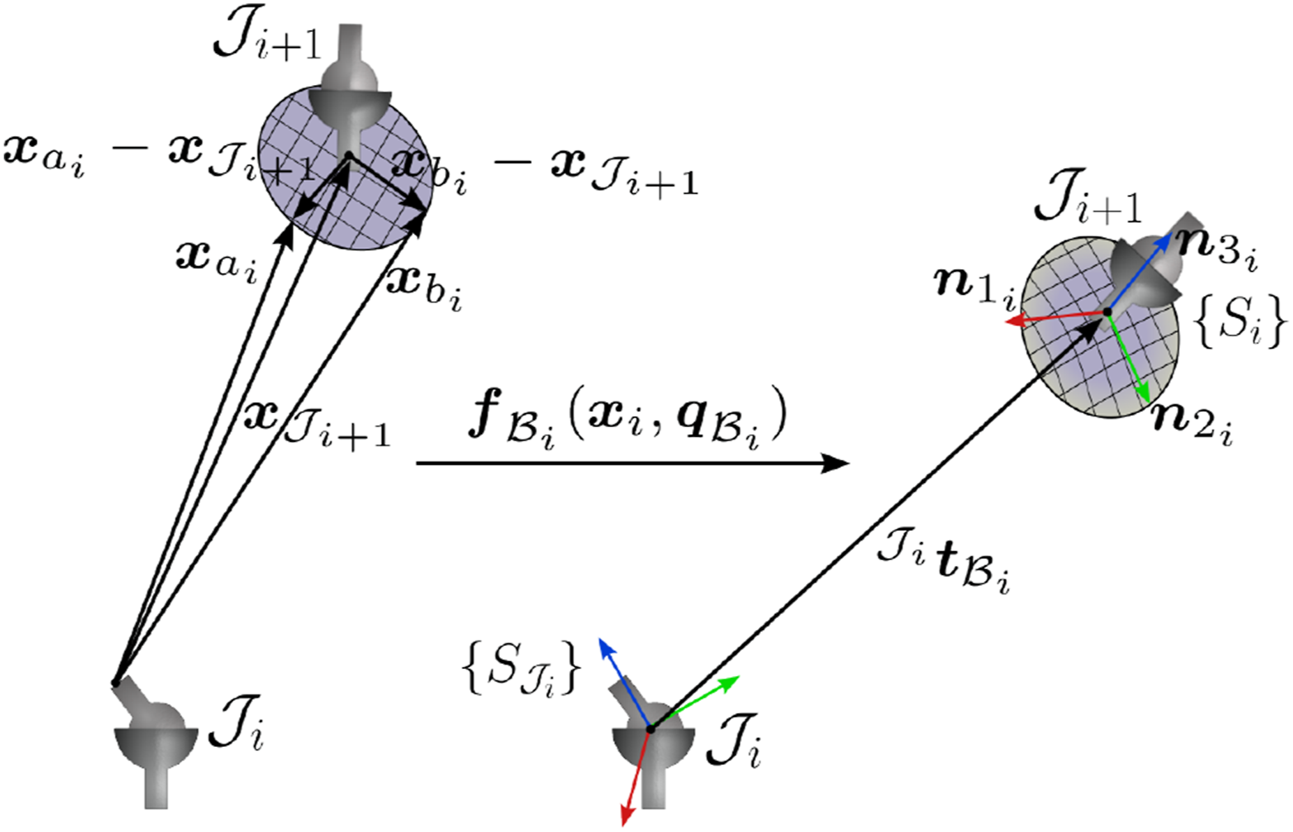
Let $x_{J_{i + 1}}$ be the pivot point of joint $J_{i + 1}$ at body $B_{i}$ , and $x_{a_{i}}$ and $x_{b_{i}}$ two points of $B_{i}$ belonging to the contact area with $J_{i + 1}$ such that

{(x_{a_{i}} - x_{J_{i + 1}})}^{T} (x_{b_{i}} - x_{J_{i + 1}}) = 0 .

(3)

By leveraging Assumption 2, it is possible to construct the homogeneous transformation matrix from {S_i} to

{S_{J_{i}}}

{}^{J_{i}}T_{B_{i}} (q_{B_{i}}) = (\begin{matrix} n_{1_{i}} & n_{2_{i}} & n_{3_{i}} & {}^{J_{i}}t_{B_{i}} \\ 0 & 0 & 0 & 1 \end{matrix}),

(4)

where

\begin{aligned} n_{1_{i}} (q_{B_{i}}) & = \frac{f_{B_{i}} (x_{a_{i}}, q_{B_{i}}) - f_{B_{i}} (x_{J_{i + 1}}, q_{B_{i}})}{‖ f_{B_{i}} (x_{a_{i}}, q_{B_{i}}) - f_{B_{i}} (x_{J_{i + 1}}, q_{B_{i}}) ‖}, \\ n_{2_{i}} (q_{B_{i}}) & = \frac{f_{B_{i}} (x_{b_{i}}, q_{B_{i}}) - f_{B_{i}} (x_{J_{i + 1}}, q_{B_{i}})}{‖ f_{B_{i}} (x_{b_{i}}, q_{B_{i}}) - f_{B_{i}} (x_{J_{i + 1}}, q_{B_{i}}) ‖}, \\ n_{3_{i}} (q_{B_{i}}) & = n_{1_{i}} \times n_{2_{i}}, \end{aligned}

(5)

and

{}^{J_{i}}t_{B_{i}} (q_{B_{i}}) = f_{B_{i}} (x_{J_{i + 1}}, q_{B_{i}}) .

(6)

The above transformation contains the information about the position and orientation of the rigid contact area between

B_{i}

and

J_{i + 1}

as seen from

J_{i}

. Figure 3 illustrates how the elements of (4) are built starting from the body kinematics (2) and the three points

x_{a_{i}}, x_{b_{i}}

and

x_{J_{i + 1}}

. Note that, without loss of generality, we choose

n_{3_{i}}

as the unit normal vector to the body-joint contact area.

It is also worth observing that (4) is a function of $q_{B_{i}}$ only because it encodes the information due to deformability. When the body is rigid, (2) reduces to the identity, that is, $p_{B_{i}} = x_{i}$ , and (4)–(6) is indeed constant. Because of Assumption 2, the orthogonality between $x_{a_{i}} - x_{J_{i + 1}}$ and $x_{b_{i}} - x_{J_{i + 1}}$ implies that between the unitary norm vectors $n_{1_{i}}$ and $n_{2_{i}}$ . Consequently, the triad ${n_{1_{i}} n_{2_{i}} n_{3_{i}}}$ forms an orthonormal basis. Moreover, (5) is always well defined since the denominators are never zero and, from Assumption 2, it holds

‖ f_{B_{i}} (x_{a_{i}}, q_{B_{i}}) - f_{B_{i}} (x_{J_{i + 1}}, q_{B_{i}}) ‖ = ‖ x_{a_{i}} - x_{J_{i + 1}} ‖,

and

‖ f_{B_{i}} (x_{b_{i}}, q_{B_{i}}) - f_{B_{i}} (x_{J_{i + 1}}, q_{B_{i}}) ‖ = ‖ x_{b_{i}} - x_{J_{i + 1}} ‖,

which are constants.

Remark 3

In some modeling approaches, such as the geometric variable strain or lumped mass models, the above transformation matrix is readily available since each point of the body is associated with a transformation matrix. However, this is not always the case as in the locally volume preserving method or reduced-order FEM.

The relative motion between $B_{i - 1}$ and $B_{i}$ due to $J_{i}$ has not been considered yet. This effect on the kinematics is modeled by the joint homogeneous transformation

{}^{B_{i - 1}}T_{J_{i}} (q_{J_{i}}) = (\begin{matrix} {}^{B_{i - 1}}R_{J_{i}} (q_{J_{i}}) & {}^{B_{i - 1}}t_{J_{i}} (q_{J_{i}}) \\ 0_{1 \times 3} & 1 \end{matrix}),

(7)

where

q_{J_{i}} \in R^{n_{J_{i}}}

is the configuration vector of the joint and

n_{J_{i}}

its number of DoFs. Note that

{}^{B_{i - 1}}T_{J_{i}} (q_{J_{i}})

is specified only by the joint type, as for rigid bodied systems (Featherstone, 2014).

For the sake of convenience, we define the vectors

q_{i} = (\begin{matrix} q_{J_{i}} \\ q_{B_{i}} \end{matrix}) \in R^{n_{i}},

with

n_{i} = n_{B_{i}} + n_{J_{i}}

, and

q = (\begin{matrix} q_{1} \\ ⋮ \\ q_{N} \end{matrix}) \in R^{n},

with

n = \sum_{i = 1}^{N} n_{i}

, which group the generalized coordinates of each body and of the entire system, respectively.

Toy Example (Continuation). We can now proceed with the computation of ${}^{J_{i}}T_{B_{i}}$ . To this end, we take the tip along the backbone as pivot point, that is, $x_{J_{i + 1}} = {(0 0 1)}^{T}$ . Moreover, the choice $x_{a_{i}} = {(1 0 1)}^{T}$ and $x_{b_{i}} = {(0 1 1)}^{T}$ guarantees the orthogonality condition (3).

Applying (4)–(6) to the CC kinematics yields

{}^{J_{i}}T_{B_{i}} = (\begin{matrix} c_{q x_{3}} & 0 & - s_{q x_{3}} & \frac{c_{q x_{3}} - 1}{q} \\ 0 & 1 & 0 & 0 \\ s_{q x_{3}} & 0 & c_{q x_{3}} & \frac{s_{q x_{3}}}{q} \\ 0 & 0 & 0 & 1 \end{matrix}),

which corresponds to the well-known transformation matrix from the tip to the base of a CC segment (Della Santina and Rus, 2019). Since the body is assumed to be connected to a fixed joint, we have

{}^{B_{i - 1}}T_{J_{i}} = I_{4} .

In the rest of the section, we present the robot forward and differential kinematics. Although the derivation introduces little new information, it is included as a necessary starting point for formulating the dynamics. We use the superscript ${}^{i}{(\cdot)}$ to indicate that a vector is expressed in the reference frame {S_i}. For ease of presentation, the superscript is omitted when the quantity is expressed in {S₀}.

3.1. Forward kinematics

Using (2), (4)–(6) and (7), we can compute the forward kinematics for all robot points. To this end, define the relative transformation from {S_i} to {S_i−1}

\begin{aligned} {}^{i - 1}T_{i} (q_{i}) & = {}^{B_{i - 1}}T_{J_{i}} (q_{J_{i}}) {}^{J_{i}}T_{B_{i}} (q_{B_{i}}) \\ = (\begin{matrix} {}^{i - 1}R_{i} & {}^{i - 1}t_{i} \\ 0_{1 \times 3} & 1 \end{matrix}), \end{aligned}

(8)

and, by concatenation, that from {S_i} to {S₀}

\begin{aligned} T_{i} (q_{1}, \dots, q_{i}) & = {}^{0}T_{1} (q_{1}) {}^{1}T_{2} (q_{2}) \dots {}^{i - 1}T_{i} (q_{i}) \\ = (\begin{matrix} R_{i} & t_{i} \\ 0_{1 \times 3} & 1 \end{matrix}) . \end{aligned}

(9)

Denote, respectively, with

{}^{i}p_{i}

and

{}^{i}p_{{C o M}_{i}} \in R^{3}

the position of a point of

B_{i}

relative to

J_{i}

and of

B_{i}

center of mass, both expressed in {S_i}. These can be computed from (2) and (4) as

\begin{aligned} {}^{i}p_{i} (x_{i}, q_{B_{i}}) & = {}^{J_{i}}T_{B_{i}}^{- 1} (\begin{matrix} f_{B_{i}} \\ 1 \end{matrix}), \end{aligned}

and

{}^{i}p_{{C o M}_{i}} (q_{B_{i}}) = \frac{1}{m_{i}} \int_{V_{i}} {}^{i}p_{i} (x_{i}, q_{B_{i}}) ρ_{i} (x_{i}) d V,

where

m_{i} = \int_{V_{i}} ρ_{i} (x_{i}) d V

is the body mass and ρ_i( x _i) its mass density. Since

{}^{i}p_{i}

and

{}^{i}p_{{C o M}_{i}}

are elements of

R^{3}

, there always exists a unique vector

{}^{i}r_{i} \in R^{3}

such that

{}^{i}p_{i} = {}^{i}r_{i} + {}^{i}p_{{C o M}_{i}},

(10)

where

{}^{i}r_{i}

satisfies the notable property

\int_{V_{i}} {}^{i}r_{i} ρ_{i} d V = \int_{V_{i}} {}^{i}p_{i} ρ_{i} d V - {}^{i}p_{{C o M}_{i}} \int_{V_{i}} ρ_{i} d V = 0_{3} .

(11)

Remark 4

In the flexible link case, ${}^{i}r_{i}$ is typically approximated following a modal-Ritz approach, that is,

{}^{i}r_{i} (q_{B_{i}}, x_{i}) = Φ_{r_{i}} (x_{i}) q_{B_{i}} .

(12)

In this work, we never consider such hypothesis. In fact, the function

f_{B_{i}}

defines a generic and possibly highly nonlinear functional dependence of

{}^{i}r_{i}

q_{B_{i}}

and x _i.

Toy Example (Continuation). Recalling that ${}^{J_{i}}T_{B_{i}} = I_{4}$ the transformation from $B_{i}$ to $B_{i - 1}$ is given by

{}^{i - 1}T_{i} =^{B_{i - 1}} T_{J_{i}} {}^{J_{i}}T_{B_{i}} =^{J_{i}} T_{B_{i}} .

Moreover, after some computations, the position vectors

{}^{i}p_{i}

{}^{i}p_{{C o M}_{i}}

and

{}^{i}r_{i}

in the body frame are

{}^{i}p_{i} = (\begin{matrix} \frac{c_{q} - 1}{q} + x_{1} c_{q} \\ x_{2} \\ - \frac{s_{q} (q x_{1} + 1)}{q} \end{matrix}), {}^{i}p_{{C o M}_{i}} = (\begin{matrix} - \frac{q - s_{q}}{q^{2}} \\ 0 \\ \frac{c_{q} - 1}{q^{2}} \end{matrix}),

and

{}^{i}r_{i} = (\begin{matrix} \frac{q c_{q} - s_{q} + q^{2} x_{1} c_{q}}{q^{2}} \\ x_{2} \\ - \frac{c_{q} - 1 + q s_{q} (q x_{1} + 1)}{q^{2}} \end{matrix}) .

We can now use (9) and (10) to describe the forward kinematics, which reads

p_{i} = p_{{C o M}_{i}} + R_{i} {}^{i}r_{i},

(13)

with

p_{{C o M}_{i}} = t_{i} + R_{i} {}^{i}p_{{C o M}_{i}} .

(14)

3.2. First- and second-order forward differential kinematics

As we will see later in Section 4, the equations of motion depend on the first- and second-order time derivatives of p _i, which we briefly introduce below. To keep the presentation concise, we provide only a minimal overview, as the derivation of the differential kinematics follows standard arguments. For a detailed derivation, we refer the interested reader to Appendix A.1.

From (13) and (14), it follows that ${\dot{p}}_{i}$ depends on the time derivatives of $t_{i}, {}^{i}p_{{C o M}_{i}}, {}^{i}r_{i}$ , namely

v_{i} = \frac{d t_{i}}{d t}, {}^{i}{\dot{p}}_{{C o M}_{i}} = \frac{d {}^{i}p_{{C o M}_{i}}}{d t}, {}^{i}{\dot{r}}_{i} = \frac{d {}^{i}r_{i}}{d t},

along with the angular velocity of {S_i}, denoted as ω _i in the following.

Similarly, the acceleration ${\ddot{p}}_{i}$ can be expressed using the terms

a_{i} = \frac{d v_{i}}{d t}, {}^{i}{\ddot{p}}_{{C o M}_{i}} = \frac{d {}^{i}{\dot{p}}_{{C o M}_{i}}}{d t}, {}^{i}{\ddot{r}}_{i} = \frac{d {}^{i}{\dot{r}}_{i}}{d t},

and

{\dot{ω}}_{i} = \frac{d ω_{i}}{d t} .

From the expression of

{\dot{p}}_{i}

and

{\ddot{p}}_{i}

(see Appendix A.1), the following lemma holds.

Lemma 1

Given $q, \dot{q}$ and $\ddot{q}$ , the first- and second-order differential kinematics expressed in the body frame, that is, ${}^{i}v_{i}, {}^{i}ω_{i}, {}^{i}v_{{C o M}_{i}}, {}^{i}a_{i}, {}^{i}{\dot{ω}}_{i}$ and $a_{{C o M}_{i}}$ , can be computed recursively forward in space from $B_{1}$ to $B_{N}$ by initializing ${}^{0}v_{0} = 0_{3} [m s^{- 1}], {}^{0}ω_{0} = 0_{3} [r a d s^{- 1}], {}^{0}a_{0} = 0_{3} [m s^{- 2}]$ and ${}^{0}{\dot{ω}}_{0} = 0_{3} [r a d s^{- 2}]$ . In addition, the computational complexity for such evaluation is O(N).

Proof. The result follows immediately by observing the recursive structure of (54)–(56) and (58)–(59).

Toy Example (Continuation). Since the expression for the differential kinematics is quite complex even in this elementary example, we omit its presentation. However, the reader can verify that velocities and accelerations in the body frame can be readily obtained from ${}^{i - 1}T_{i}$ , and the time derivatives of ${}^{i}p_{{C o M}_{i}}$ and ${}^{i}r_{i}$ .

4. Kane equations

Here, we briefly present the Kane equations for the class of robotic systems introduced in Section 2. In a nutshell, the Kane method projects the weak form of the dynamics in the configuration space by exploiting the system holonomic nature, specifically the fact that all constraints depend only on time and configuration variables, but never on their time derivatives. While the content of this section is not new per se, we believe it can be of interest to the soft robotics community, which is mostly familiar with the EL approach. We also demonstrate that the Kane and EL approach are indeed equivalent. However, as we shall see later in Section 5, the Kane equations can be manipulated to obtain a recursive form of the dynamics that can be directly used to solve Problems 1 and 2.

According to the weak form of the EoM for a continuum (Lacarbonara, 2013), for every body of the robot, one has

\int_{V_{i}} δ p_{i}^{T} (f_{{int}_{i}} + f_{{ext}_{i}} - \frac{d ({\dot{p}}_{i} ρ_{i})}{d t}) d V = 0 .

(15)

Here,

f_{{int}_{i}}

is the vector modeling internal forces per unit volume, such as the mechanical stress and actuation forces (when the system is internally actuated). The vector

f_{{ext}_{i}}

represents the resultant external force per unit volume, including, for example, gravity. Furthermore,

\frac{d ({\dot{p}}_{i} ρ_{i})}{d t}

is the time derivative of the linear momentum per unit volume.

According to the Kane method, in the computations, it suffices to consider among $f_{{int}_{i}}$ and $f_{{ext}_{i}}$ the only forces that perform work on the body in the course of a virtual displacement, that is, the forces for which $\int_{V_{i}} δ p_{i}^{T} f_{{int}_{i}} d V \neq 0$ and $\int_{V_{i}} δ p_{i}^{T} f_{{ext}_{i}} d V \neq 0$ . Thanks to the holonomic nature of the system, the reaction forces at the contact area between two bodies are non-working (Whittaker, 1964). As a result, they have no effect in the above balance equation. In other words, the internal reaction forces between adjacent bodies, either rigidly connected or in relative motion due to a joint, can be completely neglected in (15). While this equation already describes the dynamics of the body, it cannot be used in this form to compute the dynamics because it contains the virtual displacement δ p _i.

Recalling that p _i depends on q , it follows that $δ p_{i} = {(\nabla_{q} p_{i})}^{T} δ q$ . Substituting this into the above equation and rearranging the terms yields

\int_{V_{i}} δ q^{T} \nabla_{q} p_{i} (d f_{i} - \frac{d ({\dot{p}}_{i} ρ_{i})}{d t} d V) = 0,

where we have defined for compactness the net force

d f_{i} = (f_{{int}_{i}} + f_{{ext}_{i}}) d V

. Since the system is holonomic, each generalized coordinate can experience a virtual displacement independently of the others, which implies

\int_{V_{i}} \nabla_{q} p_{i} (d f_{i} - \frac{d ({\dot{p}}_{i} ρ_{i})}{d t} d V) = 0_{n} .

Summing the contributions for all body gives the reduced-order dynamics

\begin{aligned} \sum_{j = 1}^{N} \int_{V_{j}} \nabla_{q} p_{j} (d f_{j} - \frac{d ({\dot{p}}_{j} ρ_{j})}{d t} d V) = 0_{n}, \end{aligned}

and the Kane equations for the system

\begin{matrix} Q = \sum_{j = 1}^{N} \int_{V_{j}} \nabla_{\dot{q}} {\dot{p}}_{j} d f_{j}, \end{matrix}

(16)

\begin{matrix} Q^{*} = - \sum_{j = 1}^{N} \int_{V_{j}} \nabla_{\dot{q}} {\dot{p}}_{j} \frac{d ({\dot{p}}_{j} ρ_{j})}{d t} d V, \end{matrix}

(17)

\begin{matrix} Q + Q^{*} = 0_{n}, \end{matrix}

(18)

where the identity

\nabla_{q} p_{j} = \nabla_{\dot{q}} {\dot{p}}_{j}

has been used. The terms Q and Q * are called, respectively, the generalized active and inertia force because

Q = - g (q) - s (q, \dot{q}) + ν (q, u),

and

Q^{*} = - M (q) \ddot{q} - c (q, \dot{q}) .

In a nutshell, Q models all external forces, while Q * the inertia of the system. In this paper, we restrict the analysis to systems for which the variation of the mass density is negligible, that is,

{\dot{ρ}}_{i} = 0

, i ∈ {1, …, N}. This way, we can simplify the second term in the integrand of (17) to

\frac{d ({\dot{p}}_{i} ρ_{i})}{d t} d V = {\ddot{p}}_{i} ρ_{i} d V = {\ddot{p}}_{i} d m_{i},

(19)

where we defined the infinitesimal mass dm_i = ρ_idV. From (11) and the Reynolds transport theorem³, this also implies

\int_{V_{i}} {}^{i}{\dot{r}}_{i} ρ_{i} d V = \frac{d}{d t} (\int_{V_{i}} {}^{i}r_{i} ρ_{i} d V) = 0_{3},

(20)

and

\int_{V_{i}} {}^{i}{\ddot{r}}_{i} ρ_{i} d V = \frac{d}{d t} (\int_{V_{i}} {}^{i}{\dot{r}}_{i} ρ_{i} d V) = 0_{3} .

(21)

Proposition 1

Equations (16)–(19) are equivalent to (1), that is,

- Q^{*} (q, \dot{q}, \ddot{q}) = M (q) \ddot{q} + c (q, \dot{q}) = Q (q, \dot{q}, u) .

Proof. See Appendix A.2.

For the sake of the following derivations, it proves advantageous to expand Q and Q * into the rows associated to the single bodies, namely to consider the EoM (16)–(18) in the equivalent form

\begin{matrix} Q_{i} = \sum_{j = 1}^{N} \int_{V_{j}} \nabla_{{\dot{q}}_{i}} {\dot{p}}_{j} d f_{j}, \end{matrix}

(22)

\begin{matrix} Q_{i}^{*} = - \sum_{j = 1}^{N} \int_{V_{j}} \nabla_{{\dot{q}}_{i}} {\dot{p}}_{j} {\ddot{p}}_{j} d m_{j}, \end{matrix}

\begin{matrix} Q_{i} + Q_{i}^{*} = 0_{n_{i}}, \end{matrix}

(23)

with i ∈ {1, …, N}.

5. Recursive formulation of the equations of motion

This section presents the main result of the paper, that is, a recursive formulation of (22)–(23), which immediately yields a procedure for the solution of the ID problem. We provide a pseudo-code for implementing the algorithm, encompassing all necessary terms. We also show how this procedure can be modified to evaluate the mass matrix.

To this end, rewrite the left-hand side of (23) as

Q_{i} + Q_{i}^{*} = \sum_{j = 1}^{N} \int_{V_{j}} \nabla_{{\dot{q}}_{i}} {\dot{p}}_{j} (d f_{j} - {\ddot{p}}_{j} d m_{j}) .

For j < i, one has

\nabla_{{\dot{q}}_{i}} {\dot{p}}_{j} = 0_{n_{i} \times 3}

because p _j depends only on q ₁, …, q _j−1 and q _j. Thus, the lower bound (j = 1) of the above summation can be replaced with the index associated to

B_{i}

(j = i), leading to a more concise form

Q_{i} + Q_{i}^{*} = \sum_{j = i}^{N} \int_{V_{j}} \nabla_{{\dot{q}}_{i}} {\dot{p}}_{j} (d f_{j} - {\ddot{p}}_{j} d m_{j}) .

By leveraging (51), the previous equation can be rewritten as

\begin{aligned} Q_{i} + Q_{i}^{*} & = \sum_{j = i}^{N} \nabla_{{\dot{q}}_{i}} v_{{C o M}_{j}} \int_{V_{j}} d f_{j} - {\ddot{p}}_{j} d m_{j} \\ + \nabla_{{\dot{q}}_{i}} ω_{j} \int_{V_{j}} (R_{j} {}^{j}r_{j}) \times (d f_{j} - {\ddot{p}}_{j} d m_{j}) \\ + \int_{V_{j}} \nabla_{{\dot{q}}_{i}} {}^{j}{\dot{r}}_{j} R_{j}^{T} (d f_{j} - {\ddot{p}}_{j} d m_{j}) . \end{aligned}

Given that

{}^{i}r_{i}

depends only on the configuration variables of the corresponding body

B_{i}

, it holds

\nabla_{{\dot{q}}_{i}} {}^{j}{\dot{r}}_{j} = 0_{n_{i} \times 3}; j \neq i

, which simplifies the above expression to

\begin{aligned} Q_{i} + Q_{i}^{*} & = \int_{V_{i}} \nabla_{{\dot{q}}_{i}} {}^{i}{\dot{r}}_{i} R_{j}^{T} (d f_{i} - {\ddot{p}}_{i} d m_{i}) \\ + \sum_{j = i}^{N} \nabla_{{\dot{q}}_{i}} v_{{C o M}_{j}} \int_{V_{j}} d f_{j} - {\ddot{p}}_{j} d m_{j} \\ + \nabla_{{\dot{q}}_{i}} ω_{j} \int_{V_{j}} d τ_{j} - (R_{j} {}^{j}r_{j}) \times {\ddot{p}}_{j} d m_{j}, \end{aligned}

(24)

being

d τ_{j} = (R_{j} {}^{j}r_{j}) \times d f_{j}

. At this stage, it is useful to summarize what we have achieved so far. In essence, we have simplified the Kane equations in two key ways. First, we have demonstrated that the reduced-order dynamics of the i-th body does not directly depend on its predecessors, as indicated by the summation index j starting from i. Second, we have shown that the dynamics relies on three distinct types of terms. The first term captures effects local to the body. The other two account for the balance of forces and momenta with respect to the center of mass, and propagate also to the previous bodies through the summation. We now proceed with a further manipulation of the equations that will allow to obtain a recursive form.

By exploiting the invariance of the scalar product under rotations, it is possible to express (24) in the body frame {S_i} as

\begin{aligned} Q_{i} + Q_{i}^{*} & = \int_{V_{i}} \nabla_{{\dot{q}}_{i}} {}^{i}{\dot{r}}_{i} (d {}^{i}f_{i} - {}^{i}{\ddot{p}}_{i} d m_{i}) \\ + \sum_{j = i}^{N} \nabla_{{\dot{q}}_{i}} {}^{j}v_{{C o M}_{j}} \int_{V_{j}} d {}^{j}f_{j} - {}^{j}{\ddot{p}}_{j} d m_{j} \\ + \nabla_{{\dot{q}}_{i}} {}^{j}ω_{j} \int_{V_{j}} d {}^{j}τ_{j} - {}^{j}r_{j} \times {}^{j}{\ddot{p}}_{j} d m_{j}, \end{aligned}

(25)

where

d {}^{i}f_{i} = R_{i}^{T} d f_{i}

and

d {}^{i}τ_{i} = R_{i}^{T} d τ_{i}

denote the force and torque in {S_i}, respectively. For the sake of readability, we introduce the following definitions:

{}^{i}F_{i} = \int_{V_{i}} d {}^{i}f_{i}, {}^{i}{F_{i}^{*}} = - \int_{V_{i}} {}^{i}{\ddot{p}}_{i} d m_{i}, {}^{i}T_{i} = \int_{V_{i}} d {}^{i}τ_{i},

(26)

and

{}^{i}{T_{i}^{*}} = - \int_{V_{i}} {}^{i}r_{i} \times {}^{i}{\ddot{p}}_{i} d m_{i} .

(27)

Henceforth, the terms active force and torque of

B_{i}

are used to denote

{}^{i}F_{i}

and

{}^{i}T_{i}

, respectively. Similarly,

{}^{i}{F_{i}^{*}}

and

{}^{i}{T_{i}^{*}}

are its inertial force and torque. Examining the previous equations, the two active terms can be interpreted as the net external force and torque averaged over the entire body. Analogously, the inertial terms represent the time derivatives of the linear and angular momentum.

Note also that the dimension of all the above vectors is three, independently of the number of generalized coordinates.

Substituting (26) into (25) leads to the compact form

\begin{aligned} Q_{i} + Q_{i}^{*} & = \int_{V_{i}} \nabla_{{\dot{q}}_{i}} {}^{i}{\dot{r}}_{i} (d {}^{i}f_{i} - {}^{i}{\ddot{p}}_{i} d m_{i}) \\ + \sum_{j = i}^{N} \nabla_{{\dot{q}}_{i}} {}^{j}v_{{C o M}_{j}} ({}^{j}F_{j} + {}^{j}{F_{j}^{*}}) \\ + \nabla_{{\dot{q}}_{i}} {}^{j}ω_{j} ({}^{j}T_{j} + {}^{j}{T_{j}^{*}}) . \end{aligned}

(28)

The previous expression can be further simplified recalling (56), which implies that, for j = i,

\begin{aligned} \nabla_{{\dot{q}}_{i}} {}^{j}v_{{C o M}_{j}} & = \nabla_{{\dot{q}}_{i}} {}^{j}v_{j} + \nabla_{{\dot{q}}_{i}} {}^{j}ω_{j} {}^{j}{\tilde{p}}_{{C o M}_{j}} \\ + \nabla_{{\dot{q}}_{i}} {}^{j}{\dot{p}}_{{C o M}_{j}}, \end{aligned}

and, for j > i,

\begin{aligned} \nabla_{{\dot{q}}_{i}} {}^{j}v_{{C o M}_{j}} = \nabla_{{\dot{q}}_{i}} {}^{j}v_{j} + \nabla_{{\dot{q}}_{i}} {}^{j}ω_{j} {}^{j}{\tilde{p}}_{{C o M}_{j}} . \end{aligned}

Indeed, the position of the center of mass in the body frame, and consequently also its time derivative, depends only on the configuration variables of the body. The substitution of the above identities into (28) gives

Q_{i} + Q_{i}^{*} = {}^{i}π_{i} + {}^{i}{π_{i}^{*}} + M_{i},

(29)

with

\begin{align} \begin{aligned} {}^{i}π_{i} & = \int_{V_{i}} \nabla_{{\dot{q}}_{i}} ({}^{i}{\dot{r}}_{i} + {}^{i}{\dot{p}}_{{C o M}_{i}}) d {}^{i}f_{i} \\ = \int_{V_{i}} \nabla_{{\dot{q}}_{i}} {}^{i}{\dot{p}}_{i} d {}^{i}f_{i}, \end{aligned} \end{align}

(30)

\begin{align} \begin{aligned} {}^{i}{π_{i}^{*}} & = - \int_{V_{i}} \nabla_{{\dot{q}}_{i}} ({}^{i}{\dot{r}}_{i} + {}^{i}{\dot{p}}_{{C o M}_{i}}) {}^{i}{\ddot{p}}_{i} d m_{i} \\ = - \int_{V_{i}} \nabla_{{\dot{q}}_{i}} {}^{i}{\dot{p}}_{i} {}^{i}{\ddot{p}}_{i} d m_{i}, \end{aligned} \end{align}

(31)

and

\begin{aligned} M_{i} = \sum_{j = i}^{N} \nabla_{{\dot{q}}_{i}} {}^{j}v_{j} ({}^{j}F_{j} + {}^{j}{F_{j}^{*}}) + \nabla_{{\dot{q}}_{i}} {}^{j}ω_{j} \\ ({}^{j}T_{j} + {}^{j}{T_{j}^{*}} + {}^{j}{\dot{p}}_{{C o M}_{j}} \times ({}^{i}F_{j} + {}^{j}{F_{j}^{*}})) . \end{aligned}

(32)

It is easy to observe that

{}^{i}π_{i}

and

{}^{i}{π_{i}^{*}}

contain terms that depend only on

B_{i}

. As such, these terms can be computed without any recursion. In contrast,

M_{i}

involves the forces and torques of

B_{i}

as well as those of all subsequent bodies in the chain. We thus need a way to compute recursively the latter. The following theorem formalizes the main contribution of this work, namely that

M_{i}

can indeed be expressed in a recursive form.

Theorem 1

Given $q, \dot{q}$ and $\ddot{q}$ , $M_{i}; i \in {N, \dots, 1}$ , admits the following backward recursive expression

\begin{aligned} M_{i} & = \nabla_{{\dot{q}}_{i}} {}^{i}v_{i} ({}^{i}F_{i} + {}^{i}{F_{i}^{*}}) \\ + \nabla_{{\dot{q}}_{i}} {}^{i}ω_{i} ({}^{i}T_{i} + {}^{i}{T_{i}^{*}}), \end{aligned}

(33)

where

\begin{aligned} {}^{i}F_{i} + {}^{i}{F_{i}^{*}} & = {}^{i}F_{i} + {}^{i}{F_{i}^{*}} \\ + {}^{i}R_{i + 1} ({}^{i + 1}F_{i + 1} + {}^{i + 1}F_{i + 1}^{*}), \\ {}^{i}T_{i} + {}^{i}{T_{i}^{*}} & = {}^{i}T_{i} + {}^{i}{T_{i}^{*}} + {}^{i}p_{{C o M}_{i}} \times ({}^{i}F_{i} + {}^{i}{F_{i}^{*}}) \\ + {}^{i}R_{i + 1} ({}^{i + 1}T_{i + 1} + {}^{i + 1}T_{i + 1}^{*}) \\ + {}^{i}t_{i + 1} \times {}^{i}R_{i + 1} ({}^{i + 1}F_{i + 1} + {}^{i + 1}F_{i + 1}^{*}), \end{aligned}

(34)

with

{}^{N + 1}F_{N + 1} = {}^{N + 1}F_{N + 1}^{*} = 0_{3} [N]

and

{}^{N + 1}T_{N + 1} = {}^{N + 1}T_{N + 1}^{*} = 0_{3} [N m]

Proof. See Appendix A.3.

In (34), the terms ${}^{i}F_{i}$ and ${}^{i}T_{i}$ account for the total effects of the linear and angular active forces on $B_{i}$ due to $B_{i}$ itself and all its successor bodies. Similarly, ${}^{i}{F_{i}^{*}}$ and ${}^{i}{T_{i}^{*}}$ are the corresponding inertial forces. It is worth remarking that the active and inertial terms can be computed alone by setting the dual terms to zero. For example, we can obtain ${}^{i}{F_{i}^{*}}$ setting ${}^{i}F_{i} = {}^{i + 1}F_{i + 1} = 0_{3}$ in (34). Additionally, note that $\nabla_{{\dot{q}}_{i}} {}^{i}v_{i}$ and $\nabla_{{\dot{q}}_{i}} {}^{i}ω_{i}$ project the system dynamics in the direction of q _i. These projectors can be obtained seamlessly from the kinematic model because they depend only on quantities of the body. Indeed, (54) and (55) imply

\begin{aligned} \nabla_{{\dot{q}}_{i}} {}^{i}v_{i} = \nabla_{{\dot{q}}_{i}} {}^{i - 1}F_{i - 1, i} {}^{i + 1}R_{i} (q_{i}), \end{aligned}

and

\begin{aligned} \nabla_{{\dot{q}}_{i}} {}^{i}ω_{i} = \nabla_{{\dot{q}}_{i}} {}^{i - 1}ω_{i - 1, i} {}^{i + 1}R_{i} (q_{i}) . \end{aligned}

(35)

Toy Example (Continuation). Using the kinematics derived in the previous section, the projectors for a CC body are given by

\nabla_{{\dot{q}}_{i}} {}^{i}v_{i} = (\begin{matrix} \frac{c_{q} - 1}{q^{2}} \\ 0 \\ \frac{q - s_{q}}{q^{2}} \end{matrix}),

and

\nabla_{{\dot{q}}_{i}} {}^{i}ω_{i} = (\begin{matrix} 0 \\ - 1 \\ 0 \end{matrix}) .

Remark 5

Equations (29)–(35) represent a recursive form of the dynamics, parameterized by ${}^{i}π_{i}, {}^{i}{π_{i}^{*}}, {}^{i}F_{i}, {}^{i}{F_{i}^{*}}, {}^{i}T_{i}$ and ${}^{i}{T_{i}^{*}}$ . These equations hold for any soft robotic system satisfying Assumption 1.

Observe also that $M_{i}$ satisfies an important property that is useful for solving the ID problem.

Property 1

The operator $M_{i}$ is linear in all its arguments.

Proof. The property follows from (32) (or, equivalently, (34)) since the matrix and cross products are linear operators.

The above result is quite useful for our derivation since it allows isolating the contributions of the generalized active forces. In turn, this implies that Q _i and $Q_{i}^{*}$ can be computed by nullifying the inertial and active terms, respectively, that is,

Q_{i} = {}^{i}π_{i} + M_{i} ({}^{i}F_{i}, 0_{3}, {}^{i}T_{i}, 0_{3}) = - Q_{i}^{*},

(36)

and

Q_{i}^{*} = {}^{i}{π_{i}^{*}} + M_{i} (0_{3}, {}^{i}{F_{i}^{*}}, 0_{3}, {}^{i}{T_{i}^{*}}) = - Q_{i},

(37)

where the last identity in (36) and (37) arises from

Q_{i} + Q_{i}^{*} = 0_{n_{i}}

. Using the last equation and the recursive form of

M_{i}

in (33), the inertial inverse dynamics can be computed as

Q_{i} = - {}^{i}{π_{i}^{*}} - \nabla_{{\dot{q}}_{i}} {}^{i}v_{i} {}^{i}{F_{i}^{*}} - \nabla_{{\dot{q}}_{i}} {}^{i}ω_{i} {}^{i}{T_{i}^{*}} .

(38)

This expression represents the core of our ID algorithms.

5.1. Evaluation of the inertial force and torque

In this section, we address the evaluation of ${}^{i}{F_{i}^{*}}$ , ${}^{i}{T_{i}^{*}}$ and ${}^{i}{π_{i}^{*}}$ . Indeed, if these terms are known, (38) and Theorem 1 provide a way to recursively calculate Q _i, thereby solving Problem 1. In other words, thanks to Theorem 1, we can immediately solve the IID problem once the expression of the body inertial terms is available.

Using (57), ${}^{i}{F_{i}^{*}}$ takes the form

\begin{aligned} {}^{i}{F_{i}^{*}} = - {}^{i}a_{{C o M}_{i}} m_{i}, \end{aligned}

(39)

where (11) and (20)–(21) have been employed.

A similar computation for ${}^{i}{T_{i}^{*}}$ leads to

\begin{aligned} {}^{i}{T_{i}^{*}} = - \int_{V_{i}} \frac{d}{d t} ({}^{i}r_{i} \times R_{i}^{T} \frac{d}{d t} (R_{i} {}^{i}r_{i})) d m_{i} . \end{aligned}

(40)

Note that the integrand of the right-hand side represents the time derivative of the angular momentum about the center of mass. Now, using the identity

\frac{d}{d t} (R_{i} {}^{i}r_{i}) = ω_{i} \times R_{i} {}^{i}r_{i} + R_{i} {}^{i}{\dot{r}}_{i},

after some computations, (40) becomes

\begin{aligned} {}^{i}{T_{i}^{*}} & = - {}^{i}I_{i} {}^{i}{\dot{ω}}_{i} - {}^{i}ω_{i} \times {}^{i}I_{i} {}^{i}ω_{i} - {}^{i}{\dot{I}}_{i} ω_{i} - {}^{i}ω_{i} \\ \times \int_{V_{i}} {}^{i}r_{i} \times {}^{i}{\dot{r}}_{i} d m_{i} - \int_{V_{i}} {}^{i}r_{i} \times {}^{i}{\ddot{r}}_{i} d m_{i}, \end{aligned}

(41)

where we defined the body inertia

{}^{i}I_{i} = \int_{V_{i}} {}^{i}{\tilde{r}}_{i} T {}^{i}{\tilde{r}}_{i} d m_{i},

and its time derivative

{}^{i}{\dot{I}}_{i} = \frac{d {}^{i}I_{i}}{d t} = \int_{V_{i}} {}^{i}{\tilde{\dot{r}}}_{i} T {}^{i}{\tilde{r}}_{i} + {}^{i}{\tilde{r}}_{i} T {}^{i}{\tilde{\dot{r}}}_{i} d m_{i} .

Indeed, recall that, when the body is deformable,

{}^{i}r_{i}

is a function of time through q _i(t). Note also that the first two terms in the right-hand side of (41) model the rigid motion, while the remaining arise because of deformability, as expected (Stramigioli, 2024).

Now consider ${}^{i}{π_{i}^{*}}$ . By substituting (60) into (31) and performing some computations, one obtains

\begin{aligned} {}^{i}{π_{i}^{*}} = - \nabla_{{\dot{q}}_{i}} (\int_{V_{i}} {}^{i}r_{i} \times {}^{i}{\dot{r}}_{i} d m_{i}) {}^{i}{\dot{ω}}_{i} \\ + \frac{1}{2} (I_{n_{i}} \otimes ({}^{i}ω_{i}^{T} ({}^{i}ω_{i}^{T} \otimes I_{3}))) \\ v e c ({(\nabla_{q_{i}} v e c ({}^{i}{\dot{I}}_{i}))}^{T}) \\ - 2 (\int_{V_{i}} {}^{i}{\dot{r}}_{i} \times \nabla_{{\dot{q}}_{i}} {}^{i}{\dot{r}}_{i} d m_{i}) {}^{i}ω_{i} \\ - \int_{V_{i}} \nabla_{{\dot{q}}_{i}} {}^{i}{\dot{r}}_{i} {}^{i}{\ddot{r}}_{i} d m_{i} + \nabla_{{\dot{q}}_{i}} {}^{i}{\dot{p}}_{{C o M}_{i}} {}^{i}{F_{i}^{*}}, \end{aligned}

(42)

which can be computed using the differential kinematics and

F_{i}^{*}

Remark 6

All the inertial terms are functions of $q_{i}, {\dot{q}}_{i}$ and ${\ddot{q}}_{i}$ and their functional expression can be computed offline once the kinematic model of the body and its mass density are known. When a closed-form expression for the above integrals is not available, numerical integration techniques, such as the Gaussian quadrature rule, must be used. Since the numerical approximation of integrals is a distinct research area and not the focus of this work, we refer the reader to Davis and Rabinowitz (2007) and the references therein for an introduction to the topic. For the numerical results presented in the following, the integrals have been implemented through Gaussian quadrature rules with Legendre polynomials bases.

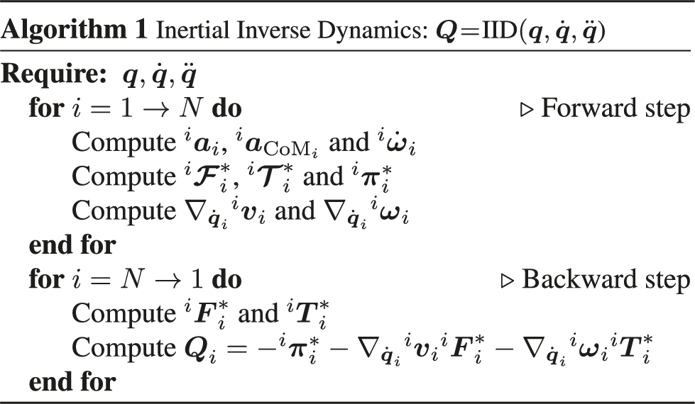
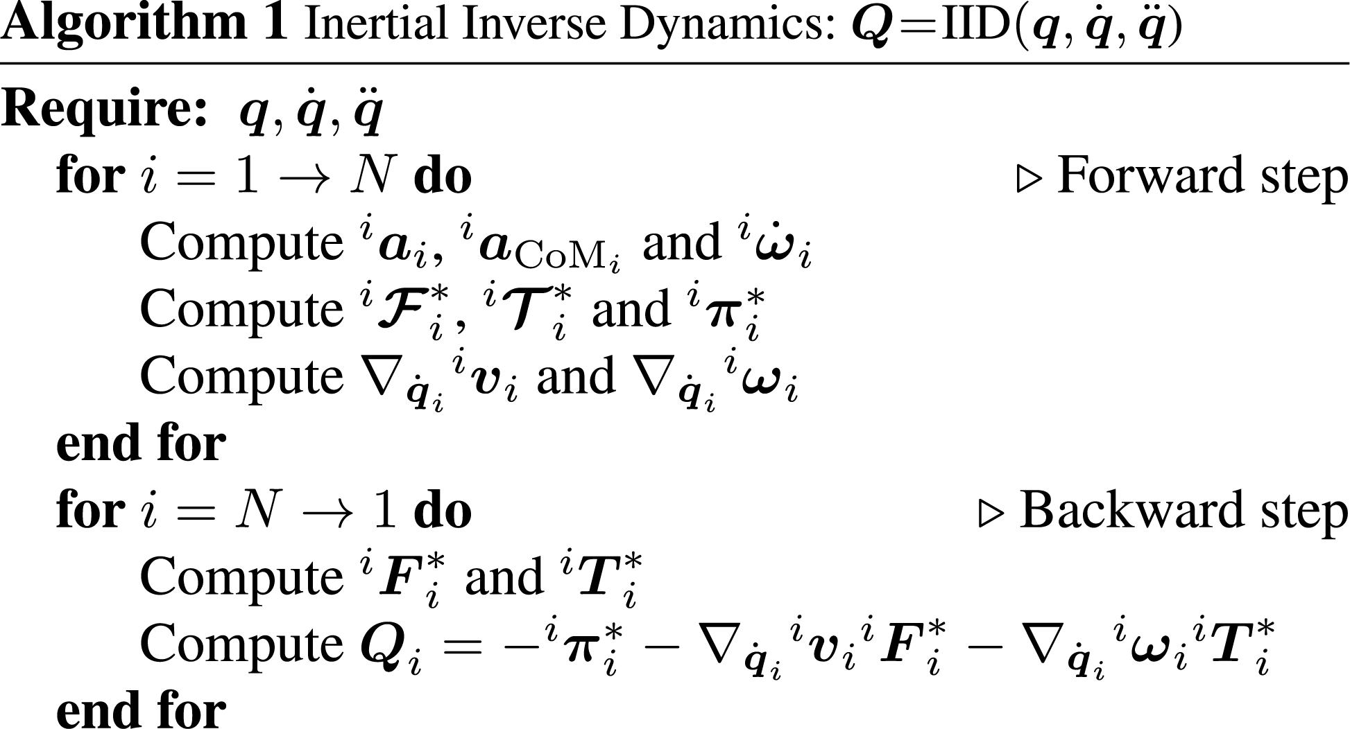
Combining all the above results, Q can be computed—and so Problem 1 solved—recursively using Algorithm 1. Analogous to the rigid body case (Featherstone, 2014), the procedure involves a forward and a backward step. In the forward step, q and its time derivatives are used to compute velocities and accelerations, enabling the evaluation of ${}^{i}{F_{i}^{*}}$ , ${}^{i}{T_{i}^{*}}$ and ${}^{i}{π_{i}^{*}}$ . At the same time, also the configuration space projectors $\nabla_{{\dot{q}}_{i}} {}^{i}v_{i}$ and $\nabla_{{\dot{q}}_{i}} {}^{i}ω_{i}$ are computed. In the backward step, the generalized inertial force is computed by projecting the inertial terms in the configuration space. This is achieved using (38) and the recursive expression for ${}^{i}{F_{i}^{*}}$ and ${}^{i}{T_{i}^{*}}$ given by (34). The computational complexity grows linearly with the number of bodies, as formalized below.

Corollary 1

The computational complexity of Algorithm 1 is O(N).

Proof. From Lemma 1, (39) and (41)–(42), the cost of the forward step in Algorithm 1 is O(N). Similarly, given the recursive form of $M_{i}$ in Theorem 1 the computational complexity of the backward step is O(N). Recall indeed that $M_{i}$ can be evaluated backward through $F_{i}^{*}$ and $T_{i}^{*}$ , which are in turn computed from the differential kinematics, $F_{i}^{*}$ and $T_{i}^{*}$ .

To better illustrate Algorithm 1 and its computational advantages over the EL approach, we present flow diagrams for both methods in Appendix A.4.

Toy Example (Continuation). According to ( 39 ) and ( 41 )–( 42 ), the inertial terms required by Algorithm 1 are derived from the kinematics and the body mass density. Assuming the latter has a unitary value, and after some simplifications, the inertial force and torque can be expressed as

{}^{i}{F_{i}^{*}} = (\begin{matrix} \frac{π (\ddot{q} q^{2} (1 - c_{q}) + 2 q s_{q} (\ddot{q} - {\dot{q}}^{2}) + 6 {\dot{q}}^{2} s_{q} - 4 {\dot{q}}^{2} q)}{q^{4}} \\ 0 \\ \frac{π ({\dot{q}}^{2} (q^{2} + 6 c_{q} - 6) + q s_{q} (2 {\dot{q}}^{2} - \ddot{q} q) - 2 \ddot{q} q c_{q})}{q^{4}} \end{matrix}),

{}^{i}{T_{i}^{*}} = (\begin{matrix} 0 \\ \frac{π}{2 q^{5}} \begin{aligned} \ddot{q} q (6 - q^{2} - 6 c_{q} - 2 q s_{q}) \\ + {\dot{q}}^{2} (- 16 + 4 q^{2} + 16 c_{q} + 4 q s_{q}) \end{aligned} \\ 0 \end{matrix}) .

Proceeding similarly for the local inertial forces yields

\begin{aligned} {}^{i}{π_{i}^{*}} = \frac{π}{6 q^{6}} (18 \ddot{q} q^{2} - \ddot{q} q^{4} + 60 {\dot{q}}^{2} s_{q} - 24 \ddot{q} q s_{q} \\ + 6 \ddot{q} q^{2} c_{q} - 12 {\dot{q}}^{2} q c_{q} - 48 {\dot{q}}^{2} q + 4 {\dot{q}}^{2} q^{3}) . \end{aligned}

All the necessary terms needed to compute the IID for a robot containing CC bodies connected are now available. Indeed, the forward step of Algorithm 1 computes ${}^{i}{F_{i}^{*}}$ , ${}^{i}{T_{i}^{*}}$ , and ${}^{i}{π_{i}^{*}}$ . These are then projected in the configuration space by $\nabla_{{\dot{q}}_{i}} {}^{i}v_{i}$ and $\nabla_{{\dot{q}}_{i}} {}^{i}ω_{i}$ during the backward step.

Note also that we have derived closed-form expressions for all terms. This implies that, for a robot with planar CC bodies, the ID can be computed analytically for an arbitrary number of bodies using Algorithm 1.

In the case where the system contains only rigid bodies, the IID for rigid robots are immediately recovered, as one might expect.

In assessing the computational complexity of Algorithm 1, we do not account for the cost of evaluating the intra-body terms, that is, those that depend on the body kinematics (8). However, in practice, the computational resources required for their evaluation may be significant. For an analysis of how kinematics affects the computation of the ID, the interested reader is referred to Appendix A.5.

Remark 7

Similar to ID algorithms for rigid robots (Featherstone, 2014), Algorithm 1 is well-suited for parallelization. Indeed, the relative kinematic and dynamic terms, such as $\nabla_{{\dot{q}}_{i}} {}^{i}v_{i}$ and ${}^{i}{π_{i}^{*}}$ , can be evaluated in a parallel loop prior to executing the forward and backward steps of Algorithm 1. Their computation typically accounts for the majority of the processing time. This is primarily due to the need for repeated evaluations of highly nonlinear functions that depend on the kinematics (2), which cannot be accelerated since the latter is treated as a black-box. Therefore, significant attention should be devoted to implementing these terms as efficiently as possible.

5.2. O(N) computation of M(q)

We now discuss how Algorithm 1 can be modified to compute the generalized mass matrix M ( q ) alongside the generalized active force Q in O(N) steps.

First, observe that

M (q) \ddot{q} = IID (q, 0_{n}, \ddot{q}),

which implies

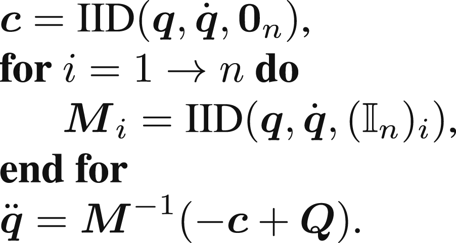
M (q) = J_{\ddot{q}} IID (q, 0_{n}, \ddot{q}) = - J_{\ddot{q}} {π^{*}}^{0} - J_{\ddot{q}} M^{0},

(43)

where the superscript ⁰ on π * and

M

indicates that these terms are computed with zero velocity. In other words, the evaluation of M ( q ) can be performed by setting the velocities to zero and differentiating both π * and

M

with respect to

\ddot{q}

. It is worth noting that the idea of exploiting the linearity of the dynamics in the accelerations to evaluate the mass matrix has already been proposed for rigid manipulators, both in configuration space (Pu et al., 1996; Rodriguez and Kreutz-Delgado, 1992) and task space (Lilly and Orin, 1990). However, to the best of our knowledge, this is the first time such a method is discussed for robots with deformable bodies. We also propose embedding the computation of M directly into the ID process because it has minimal impact on computation time while providing greater flexibility for control purposes. In Appendix A.6, we detail how M can be computed alongside Q and present a new algorithm called Mass Inertial Inverse Dynamics (MIID) for this computation.

Having a procedure that allows evaluating also M while solving the ID offers two benefits. First, it enables the computation of nonlinear control techniques for underactuated mechanical systems (Spong, 1994), such as continuum soft robots, and variable gain PD control (Della Santina and Albu-Schaeffer, 2020; Santibañez and Kelly, 2001; Wotte et al., 2023) with a single call to the ID. Second, it provides a means of solving the FD problem, that is, given $q, \dot{q}$ and $Q (q, \dot{q}, u)$ compute $\ddot{q}$ , with a significant speedup over the inertia-based algorithm (IBA) (Featherstone, 2014). Computing forward dynamics using an ID procedure, whether the MIID or the IBA, is never optimal. Nonetheless, it is worth mentioning this class of approaches because they are almost effortless to implement and have been used in the simulations of this paper.

Given the MIID, one can solve the FD in two steps

$(c, M) = M I I D (q, \dot{q}, 0_{n})$ ,

$\ddot{q} = M^{- 1} (- c + Q)$ .

Recall that, in the above algorithm, Q is known because we are solving the FD problem. On the other hand, in the IBA, $\ddot{q}$ is computed in three stages

Because of the mass matrix inversion, the complexity for solving the FD with the MIID is the same as that of the IBA, namely O(N³). However, in the IBA, the computation of M requires n calls to the ID, resulting in a O(N²) cost. Additionally, the kinematic and inertial terms must be re-evaluated at every call with an obvious waste of computational resources. When the body geometry is complex, the computation of these terms can easily become a bottleneck and exceed the time required for matrix inversion, especially if the total number of DoFs remains in the order of tens, as is customary in ROMs for control purposes.

6. Inverse dynamics

After solving Problem 1, we now demonstrate how to solve the ID problem (Problem 2). At this stage, the ID can be conceptually addressed by leveraging the IID algorithm and Property 1 to separate, without affecting computational complexity, the effects of the actuators from those of other active forces, such as the gravitational load and the interaction forces due to body deformability.

Specifically, being elements of vector spaces, $d {}^{i}f_{i}$ and $d {}^{i}τ_{i}$ can be decomposed in the forces and torques acting on the body. This paper considers, other than actuation, two additional types of active forces, namely gravitational and visco-elastic forces. Thus, the active force and torque take the form

d {}^{i}f_{i} = d^{i} f_{i}^{g} + d^{i} f_{i}^{s} + d^{i} f_{i}^{a},

(44)

and

d {}^{i}τ_{i} = d^{i} τ_{i}^{s} + d^{i} τ_{i}^{a},

(45)

where

d^{i} f_{i}^{g}

d^{i} f_{i}^{s}

and

d^{i} f_{i}^{a}

denote the force due to gravity, stress and actuation, respectively. The vectors

d^{i} τ_{i}^{s}

and

d^{i} τ_{i}^{a}

represent their rotational counterparts. Note that the effect of gravity appears only as a linear force, namely

d^{i} τ_{i}^{g} = 0_{3}

. Recalling the definition of Q _i in (22) and the subsequent derivations, the generalized active force is

Q_{i} (q, \dot{q}, u) = - g_{i} (q) - s_{i} (q, \dot{q}) + ν_{i} (q, u),

(46)

where each term in the right-hand side of the equation is obtained by replacing d f _i and d τ _i with the corresponding force and torque as in (44) and (45). We can now compute the ID replacing (46) into (23) as

ν_{i} = g_{i} (q) + s_{i} (q, \dot{q}) - Q_{i}^{*},

or, equivalently by using (36)–(37) and the linearity of

M_{i}

(Property 1),

\begin{aligned} ν_{i} = - {}^{i}{π_{i}^{*}} - {}^{i}π_{i}^{g} - {}^{i}π_{i}^{s} \\ - M_{i} ({}^{i}F_{i}^{g} + {}^{i}F_{i}^{s}, {}^{i}{F_{i}^{*}}, {}^{i}T_{i}^{s}, {}^{i}{T_{i}^{*}}), \end{aligned}

with

{}^{i}F_{i}^{{g, s}}

and

{}^{i}T_{i}^{s}

obtained recursively by using

{}^{i}F_{i}^{{g, s}}

and

{}^{i}T_{i}^{s}

in (34). The last two terms and

{}^{i}π_{i}^{{g, s}}

are obtained replacing the respective infinitesimal forces and torques into (26)–(27) and (30), respectively. We address their computation in the following subsections.

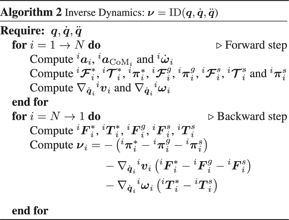
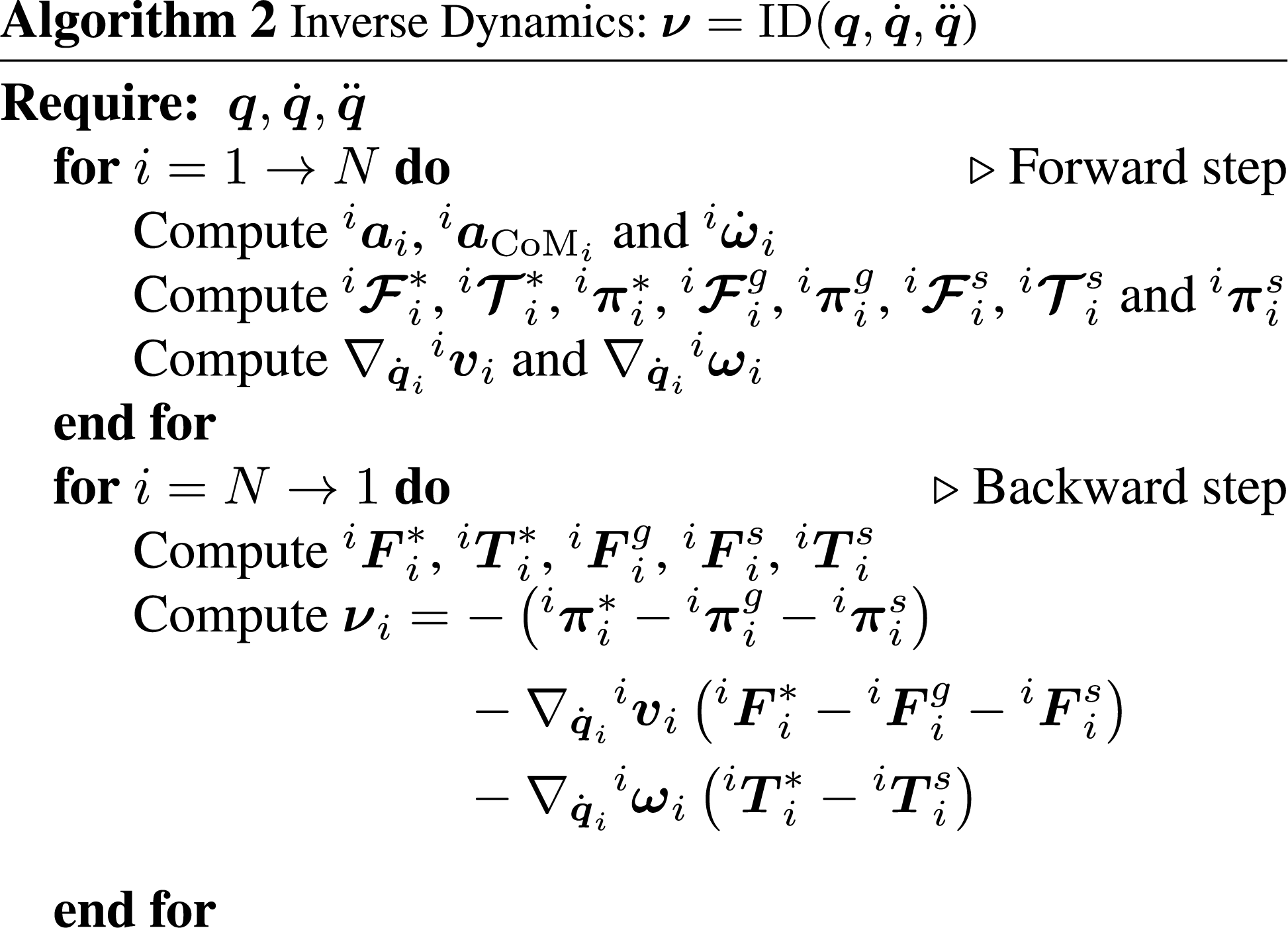
The pseudo-code for the computation of ν _i is given in Algorithm 2, which is similar to that of the IID. The difference lies in accounting for the terms that correspond to active forces which are not those generated by actuation. Note that it is possible to embed the computation of the mass matrix also in Algorithm 2 by using the same recursive formulas of the Jacobians presented in Appendix A.6 for Algorithm 1 and leading to an algorithm analogous to the MIID, denoted later as Mass Inverse Dynamics (MID).

6.1. Gravitational force

In the following, we focus on computing the gravitational load, which is obtained by considering the gravitational force acting on an infinitesimal volume element of the body and by integrating over the entire body volume.

Specifically, the gravitational active force performing work on $B_{i}$ is

F_{i}^{g} = \int_{V_{i}} R_{i}^{T 0} g d m_{i} = R_{i}^{T 0} g m_{i} = {g m}_{i}^{i},

(47)

being ⁰

g \in R^{3}

the gravity vector in {S₀} and ⁱ g its representation in body coordinates. Similarly, we have

{}^{i}π_{i}^{g} = \nabla_{{\dot{q}}_{i}} {}^{i}{\dot{p}}_{{C o M}_{i}} {}^{i}{g m}_{i} .

(48)

The computation of

{}^{i}F_{i}^{g}

can be performed sequentially from the first body to the last. However, by comparing (47) with (39) and (48) with (42), it is possible to see that the effect of gravity can be incorporated into the calculations by setting the acceleration of the base to

{}^{0}a_{0} = -^{0} g

Toy Example. (Continuation). Under the assumption that the robot base is rotated so that the gravitational force acts along the Z direction, that is, ⁰ $g = {(0 0 g_{0})}^{T}$ , the above terms become

{}^{i}F_{i}^{g} = (\begin{matrix} - π g_{0} s_{q} \\ 0 \\ - π g_{0} c_{q} \end{matrix}),

and

{}^{i}π_{i}^{g} = - \frac{π g_{0} (2 c_{q} + q s_{q} - 2)}{q^{3}} .

6.2. Visco-elastic force

As final step in evaluating the ID, we assess visco-elastic generalized forces, which model the tendency of a continuum to return in its undeformed configuration. The derivation of these force requires necessarily further hypotheses because a stress-strain model is required. In the following, we assume that $s_{i} (q, \dot{q}) = k_{i} (q) + d_{i} (q, \dot{q})$ , and denote the corresponding infinitesimal forces (torques) as $d^{i} f_{i}^{e}$ $(d^{i} τ_{i}^{e})$ and $d^{i} f_{i}^{d}$ $(d^{i} τ_{i}^{d})$ , respectively. Furthermore, let

{}^{i}B_{i} = J_{x_{i}} f_{B_{i}} {(J_{x_{i}} f_{B_{i}})}^{T},

the Green strain tensor. Assuming an incompressible Neo-Hookean solid one has

d^{i} f_{i}^{e} = 2 C_{i} {div}_{x_{i}} {}^{i}B_{i} d V,

and

d^{i} τ_{i}^{e} = {}^{i}r_{i} \times d^{i} f_{i}^{e},

where C_i is a material parameter. Note that the divergence operator projects the internal stress into the dynamic equations (Lacarbonara, 2013). Similarly, considering a Kelvin–Voigt model for the viscous forces leads to

d^{i} f_{i}^{d} = η_{i} C_{i} {div}_{x_{i}} {}^{i}{\dot{B}}_{i} d V,

and

d^{i} τ_{i}^{d} = {}^{i}r_{i} \times d^{i} f_{i}^{d},

being η_i the material damping factor.

Finally, ${}^{i}F_{i}^{{e, d}}$ , ${}^{i}T_{i}^{{e, d}}$ and ${}^{i}π_{i}^{{e, d}}$ can be obtained by proper integration over the body domain using (26)–(27) and (30).

Toy Example. (Continuation). It can be shown that (Armanini et al., 2023), for the above stress-strain model, the visco-elastic force is linear and takes the form $s_{i} = π / 4 (q - \dot{q})$ , assuming again unitary values for elastic and damping parameters.

Remark 8

Many different stress-strain models could have been considered. Indeed, from Property 1, a different model of these forces will affect only the computation of s _i.

7. Numerical results

The main contribution of this work is a unified and model-agnostic procedure to evaluate the ID of soft robots ROMs for control purposes. The previous algorithms are validated through numerical simulations, which are illustrated below. Experimental validation is beyond the scope of this paper and will be considered in future work. Additionally, it is important to keep in mind that the derived ID procedures, by design, do not depend on the specific kinematic model used and produce dynamics equivalent to the EL equations, as proven in Appendix A.2. Therefore, the accuracy of the dynamic models obtained with our algorithms is equivalent, up to numerical precision, to that of the EL approach, which primarily depends on the accuracy of the underlying kinematic model. For the same reasons mentioned above, we decided not to validate our method using open-source datasets available in the literature, such as Grassmann et al. (2022).⁴

Below, we utilize the MID algorithm described in Section 5.2 to simulate—despite this is not its intended use—and control a soft continuum robot with 3D bodies and a hybrid rigid-soft manipulator. In both simulations, we use a kinematic model based on LVP primitives (Xu and Chirikjian, 2023). It is the first time such model is used for dynamic simulation and thus also this section presents a (small) contribution of the paper. Through these simulations we also show the benefit from a control perspective of including the computation of M in the solution of the ID problem. In a third simulation, we compare the computation time of the IID algorithm with that of the EL equations to show the scalability of the recursive EoM.

The same ID algorithm is used in all the following simulations. Every simulation is implemented by providing a different robot model to the procedure. The simulations are implemented in MATLAB through Jelly, an object-oriented library offering C/C++ code generation functionality both in the MATLAB and Simulink environment.

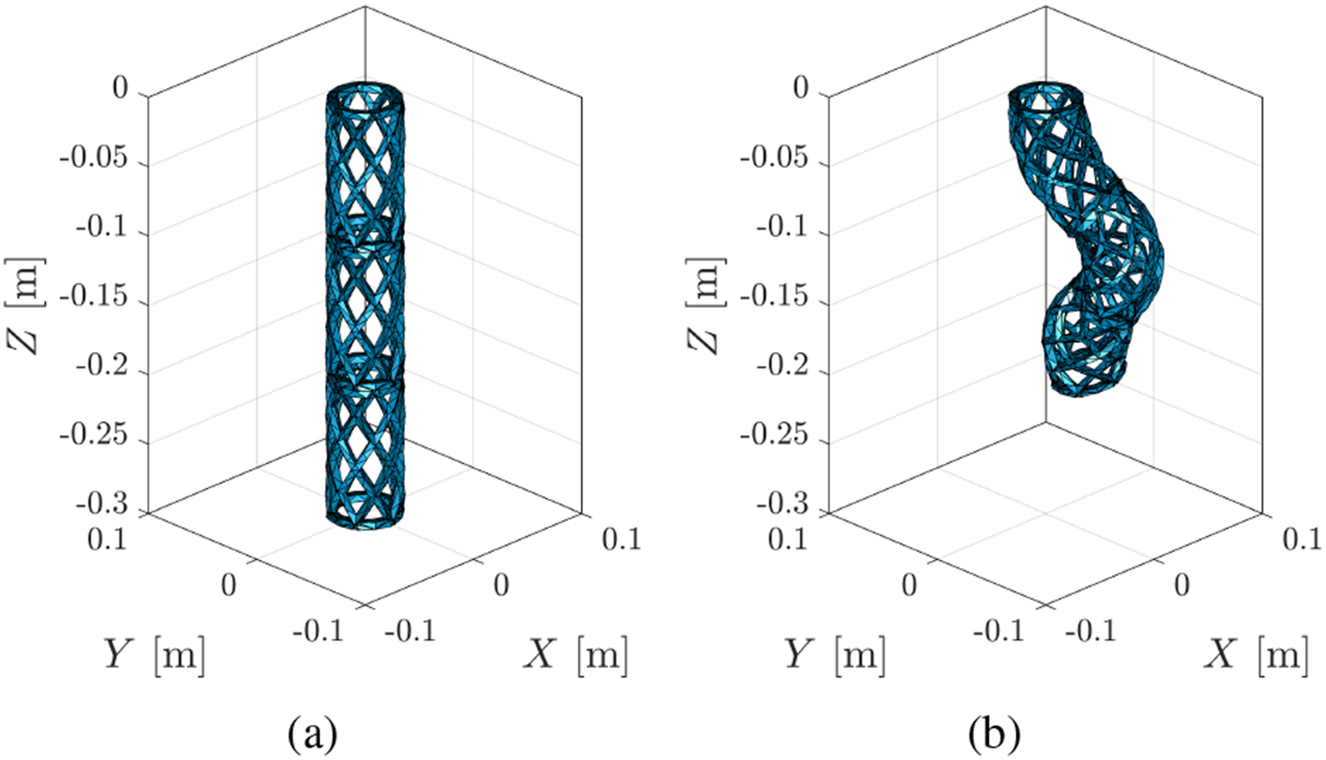
7.1. Simulation 1: Trimmed helicoid continuum soft robot

We consider the task of controlling a trimmed helicoid continuum soft robot inspired by Guan et al. (2023) and illustrated in Figure 4. These soft robotic systems do not satisfy the Cosserat rod assumption because they deform in all directions. As a consequence, other kinematic models should be considered to capture the system motion. The robot consists of three helical bodies of rest length L_i = 10 ⋅ 10⁻² [m] and radius 2 ⋅ 10⁻² [m]. The base is rotated so that the arm is aligned with the gravitational field in the straight configuration. Each body has uniform mass distribution ρ_i = 960 [kg m⁻³], elastic parameter C_i = 0.178 [MPa] and damping coefficient η_i = 0.05 [s]. The robot is actuated through nine straight tendons, running in triplets from one body to its successor and routed along their external perimeters. The kinematics is modeled using LVP primitives (Xu and Chirikjian, 2023), a new reduced-order FEM-like approach for modeling soft robots that has been simulated only in static conditions. The primitives are functions $h_{p} (x_{i}, q_{B_{i}}) \in R^{3}; p \in {1, \dots, P}$ modeling elementary types of deformation and satisfying the property that det( J _x h _p) = 1 so that volume is locally preserved. Given a set of primitives, the body kinematics is obtained by function composition leading to

f_{B_{i}} (x_{i}, q_{B_{i}}) = h_{P} (h_{P - 1} (\dots h_{1} (x_{i}, q_{B_{i}}), q_{B_{i}}), q_{B_{i}}),

which is a highly nonlinear function in both arguments. It is worth remarking that ID algorithms for flexible bodies or discrete Cosserat rods are not suitable for solving the ID problem for such kinematics. We consider six different types of LVP primitives, namely elongation, bending, shear and twist.

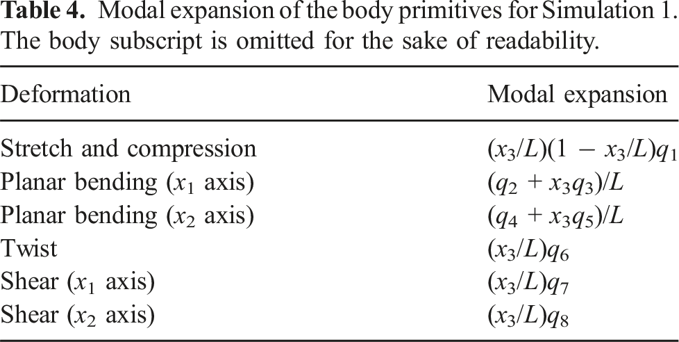
Table 4 summarizes, for each primitive, the modes functions used, which provide eight DoFs to each body. We refer the reader to Xu and Chirikjian (2023) for the functional structures of the primitives and more details on this modeling approach. Given that the motion of the system is parameterized by a finite number of configuration variables, the dynamics takes the form of (1), namely

M (q) \ddot{q} + c (q, \dot{q}) + g (q) + s (q, \dot{q}) = ν (q, u) = A (q) u,

where

q \in R^{24}

A (q) \in R^{24 \times 9}

is the actuation matrix projecting the control inputs into the configuration space and

u \in R^{9}

denotes the vector of actuation inputs, that is, the tendons tensions. The actuation matrix is computed using the principle of virtual work, following steps similar to those of Renda et al. (2022), as

δ q^{T} ν (q, u) = δ l {(q)}^{T} u = δ q^{T} A (q) u,

where l ( q ) is the actuator length in the given configuration. Thus, the robot is highly underactuated with a 15 degree of underactuation. We use the stress-strain model described in Section 6.2. More accurate and sophisticated actuation and stress-strain models could have been considered. Here, we choose a reasonable balance between fidelity and applicability for control purposes. The volume integrals appearing in the ID algorithms are computed numerically using meshes of 2749 tetrahedrons for each body.

Table 4.

Modal expansion of the body primitives for Simulation 1. The body subscript is omitted for the sake of readability.

Deformation	Modal expansion
Stretch and compression	(x₃/L)(1 − x₃/L)q₁
Planar bending (x₁ axis)	(q₂ + x₃q₃)/L
Planar bending (x₂ axis)	(q₄ + x₃q₅)/L
Twist	(x₃/L)q₆
Shear (x₁ axis)	(x₃/L)q₇
Shear (x₂ axis)	(x₃/L)q₈

The control problem consists in following three circular trajectories assigned at the bodies tips. The commanded references in the robot base coordinates are (in [m])

t_{1_{d}} = (\begin{matrix} 0.02 \cos (\frac{2 π}{5} t) \\ 0.02 \sin (\frac{2 π}{5} t) \\ 0.08 \end{matrix}), t_{2_{d}} = (\begin{matrix} 0.025 \cos (\frac{2 π}{5} t) \\ 0.025 \sin (\frac{2 π}{5} t) \\ 0.15 \end{matrix}),

and

t_{3_{d}} = (\begin{matrix} 0.030 \cos (\frac{2 π}{5} t) \\ 0.030 \sin (\frac{2 π}{5} t) \\ 0.24 \end{matrix}) .

Given the highly underactuation, the derivation of a Cartesian controller with proven stability guarantees is not straightforward and not addressed yet in the control literature. We thus solve the control problem in two steps. First, the Cartesian trajectory $t_{d} = {(t_{1_{d}}^{T} t_{2_{d}}^{T} t_{3_{d}}^{T})}^{T}$ is sampled and used to solve a static problem, which provides the unique equilibrium compatible with the unactuated dynamics for the given reference. Remarkably, the ID procedure offers a mean of efficiently solving also the statics since, in a robot equilibrium, the following holds

g (q_{e q}) + s (q_{e q}, 0) + A (q_{e q}) u_{e q} (q_{e q}) = 0_{n},

(49)

where u _eq( q _eq) is the actuation force—here obtained from a Cartesian regulator—and q _eq the unknown equilibrium. Specifically, the above equation can be solved numerically with a Newton–Raphson routine calling iteratively Algorithm 2. The equilibria, obtained by solving (49) at the sampled time instants, are then interpolated into a twice differential trajectory and converted into a smooth reference y _d(t) for the actuation coordinates (the tendons elongation inside the robot), which are then commanded through a Partial Feedback Linearization (PFBL) on the collocated dynamics (Pustina et al., 2024). Thanks to the stability of the zero dynamics (Pustina et al., 2022), the controller guarantees proven global exponential stability and takes the form

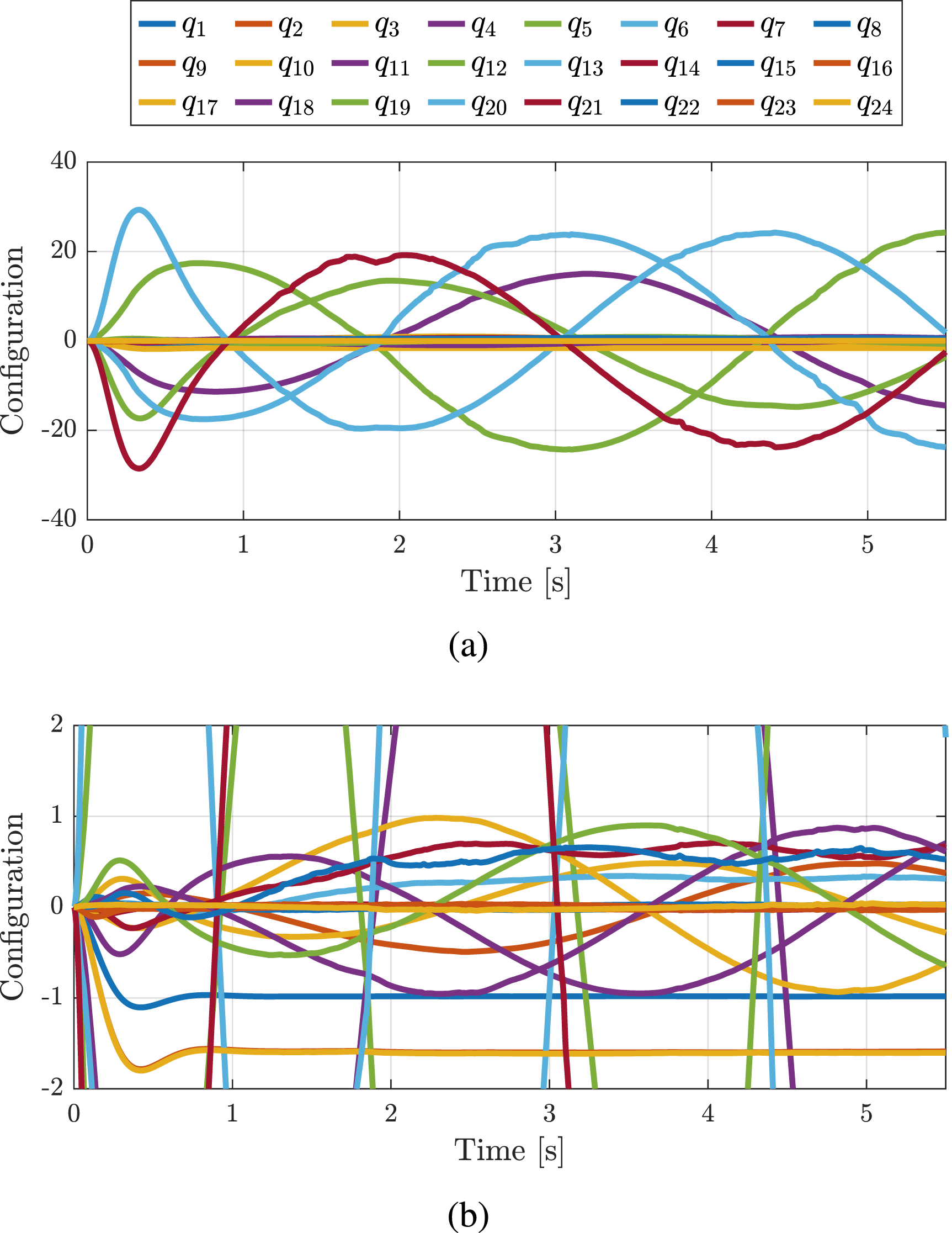
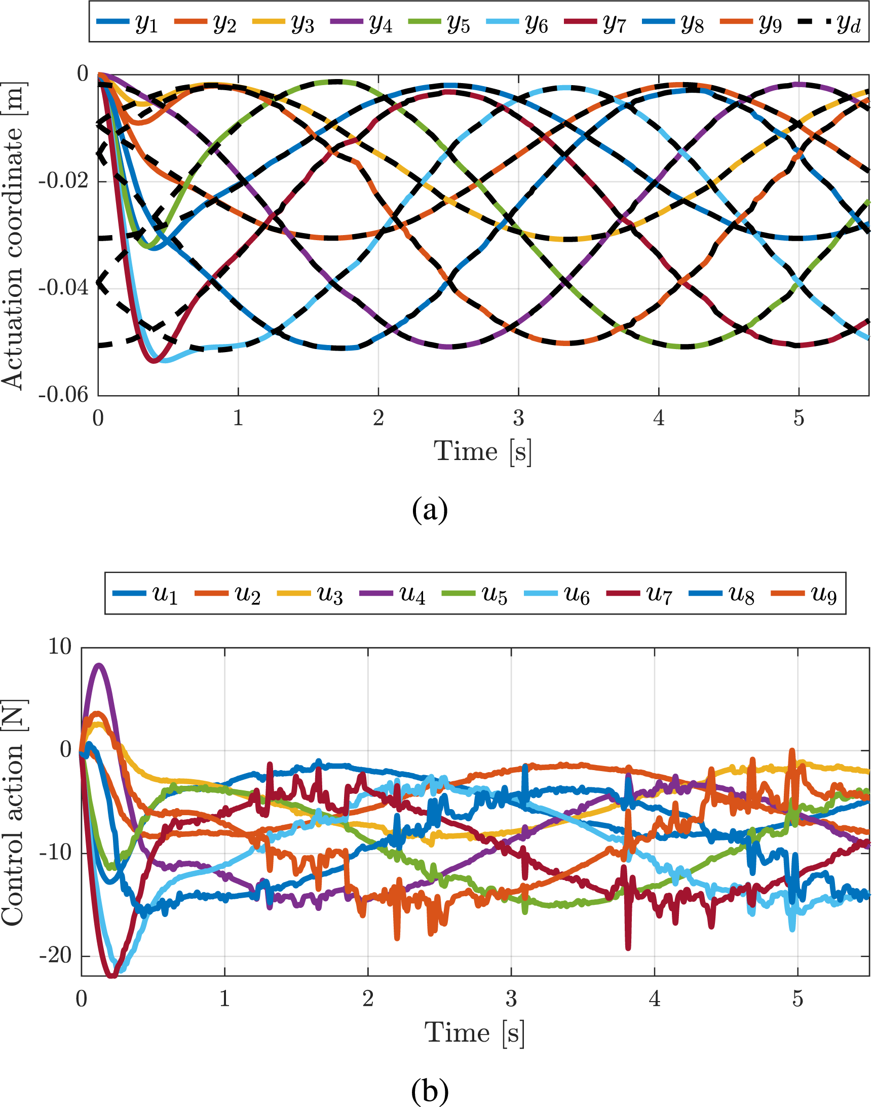
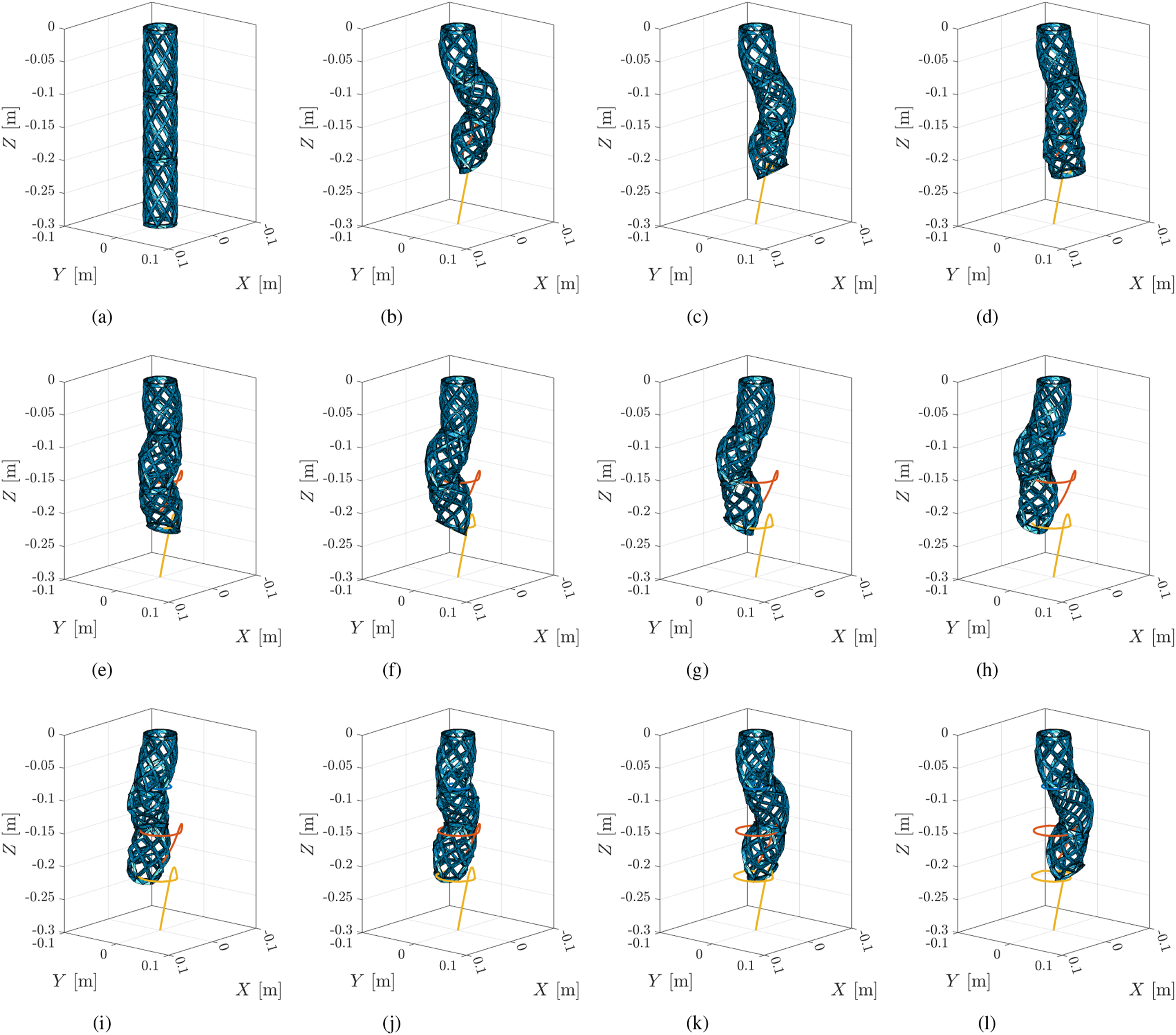
\{\begin{aligned} u & = (M_{a a}^{θ} - M_{a u}^{θ} {M_{u u}^{θ}}^{- 1} M_{u a}^{θ}) a + c_{a}^{θ} \\ - M_{a u}^{θ} {M_{u u}^{θ}}^{- 1} (c_{u}^{θ} + g_{u}^{θ} + s_{u}^{θ}), \\ a & = {\ddot{y}}_{d} + K_{D} ({\dot{y}}_{d} - \dot{y}) + K_{P} (y_{d} - y), \end{aligned}

where the system dynamics—expressed through the superscript (⋅)^θ in the decoupling coordinates θ = ( y ^T z ^T) with

z \in R^{n - m}

a complement to y —has been partitioned in actuated and unactuated part, and

K_{P} = 10 \cdot I_{9} [N]

and

K_{D} = 1 \cdot I_{9} [Ns]

are the control gains. The dynamic terms needed for the computation of the control action can be obtained with a single call to the MID as

M I D (q (θ), \dot{q} (θ, \dot{θ}), 0_{n})

. Note the appearance of M in the above control law and so the utility of having a ID procedure that allows the computation of M as well. Figures 5 and 6 show the time evolution of the configuration variables, and of the actuation coordinates and of the control action, respectively. As expected, y converges exponentially fast to y _d. In Figure 7, we illustrate snapshots of the robot motion in its workspace during the execution of the task.

7.2. Simulation 2: Hybrid rigid-soft robotic arm

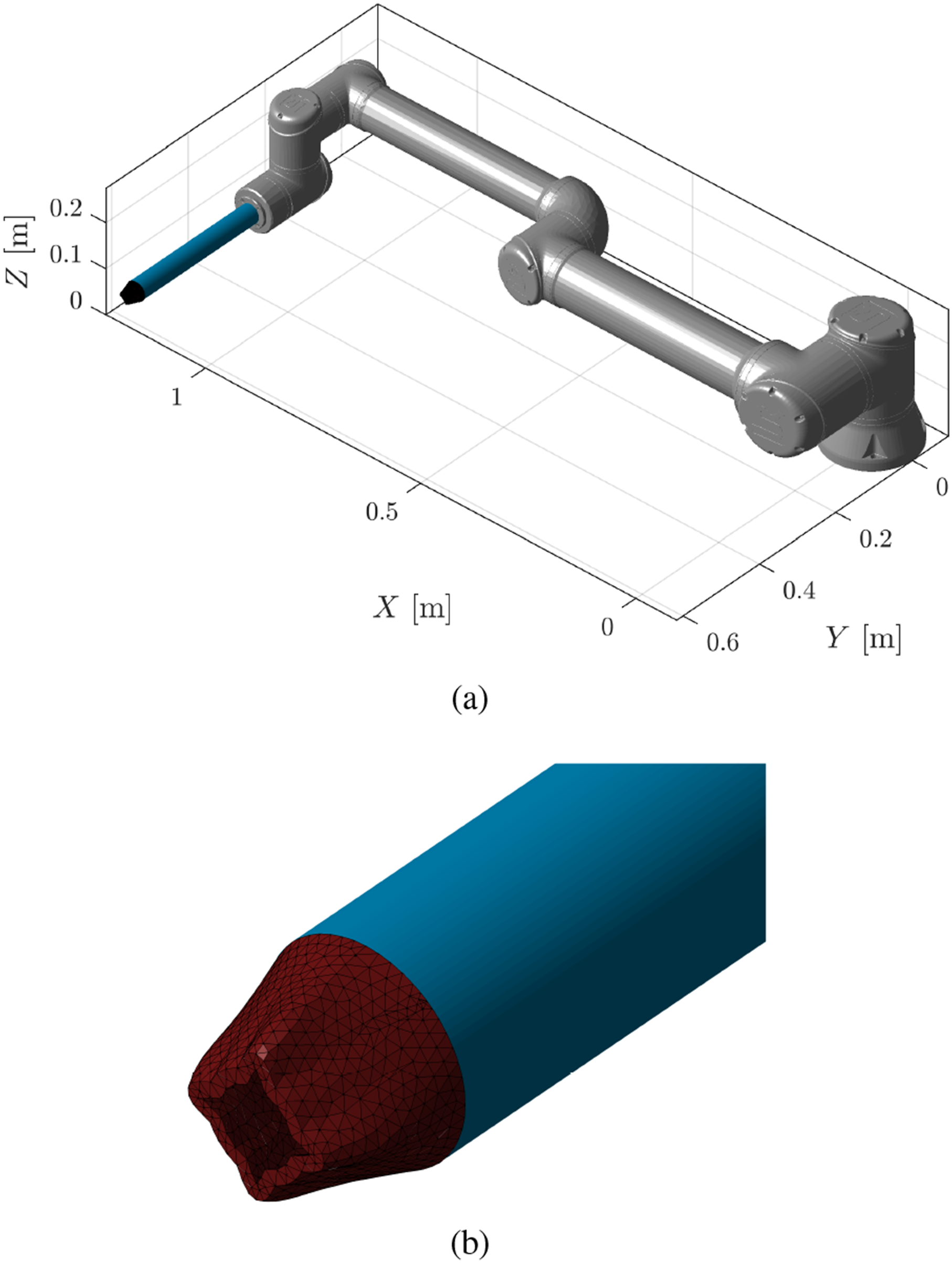
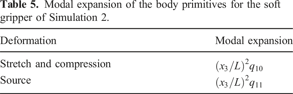
In this simulation, we demonstrate how the proposed approach can handle robots with rigid and soft bodies, each possibly modeled using different kinematics. We consider a hybrid manipulator including a Universal Robot UR10e, a slender continuum soft arm modeled as a Cosserat rod with the GVS approach (Boyer et al., 2020), and a soft gripper modeled as a 3D continuum with LVP primitives. The setup, which consists of N = 8 bodies, is illustrated in Figure 8. The gravitational force acts along the negative direction of the z-axis. The soft arm has radius 0.02 [m], rest length 0.3 [m], mass density 1070 [kg m⁻³]. The material elastic and damping coefficients are 0.17857 [MPa] and 0.1 [s], respectively. Three tendons displaced by an angle of 120° and at a distance from the center backbone of 0.015 [m] actuate the Cosserat segment. For the sake of simplicity, its backbone strain is modeled under the piecewise constant curvature hypothesis with elongation, thus resulting in three DoFs for this body. The effect of actuation is modeled as in Renda et al. (2022). On the other hand, the soft gripper has mass density 960 [kg m⁻³], elastic coefficient 22.2 [MPa], and damping factor 0.05 [s]. The gripper kinematics is modeled with two LVP primitives: an elongation primitive and a cavity primitive. The first accounts for the compression when the gripper closes and the second for the radial change due to inflation of the inner air chamber. The mode functions used by these primitives are reported in Table 5.

Table 5.

Modal expansion of the body primitives for the soft gripper of Simulation 2.

Deformation	Modal expansion
Stretch and compression	${(x_{3} / L)}^{2} q_{10}$
Source	${(x_{3} / L)}^{2} q_{11}$

Because the gripper is the last body in the chain, Assumption 2 can be relaxed to allow deformation of the top area. Thus, we allow for the mode functions of both primitives to be nonzero at the body distal end, that is, when x₃ = L. The gripper is actuated by applying a pressure difference with respect to the atmospheric one. This input is projected into the configuration space using the top and lateral surface area of the pressurized chamber.

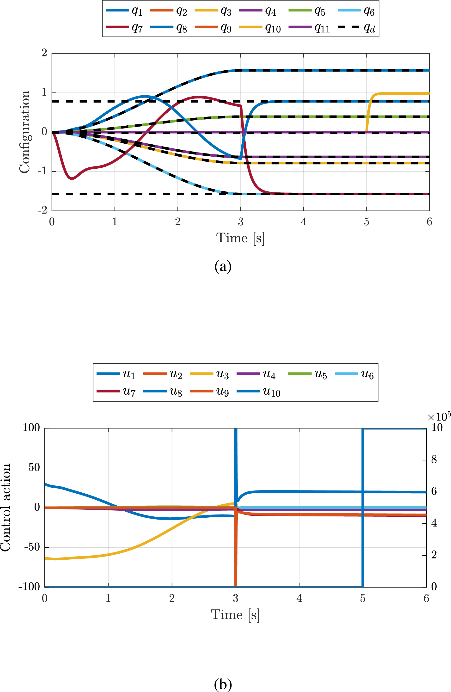
The control task involves using both rigid and deformable bodies to navigate the environment and grasp an object with the end-effector. This task is divided into three sub-tasks: (i) track a rest-to-rest cubic joint trajectory for the UR10e between

q_{i_{UR 10 e}} = {(\begin{matrix} 0 & 0 & 0 & 0 & 0 & 0 \end{matrix})}^{T},

and

q_{f_{UR 10 e}} = {(\begin{matrix} π / 2 & - π / 4 & - π / 4 & - π / 5 & π / 8 & - π / 2 \end{matrix})}^{T},

while keeping the soft bodies passive, (ii) perform a swing-up motion with the soft segment to the final configuration

q_{f_{GVS}} = {(\begin{matrix} - π / 2 & π / 4 & - 0.02 \end{matrix})}^{T},

and (iii) close the gripper. Each task is executed sequentially within three time windows t₁ ∈ [0, 3) [s], t₂ ∈ [3, 5) [s], and t₃ ∈ [5, 6] [s]. Sub-task (i) is solved with a PFBL similar to that of Simulation 1. However, in this case, the controller can be implemented directly into the configuration space since the actuation coordinates correspond to the joint angles. The control gains are chosen as

K_{P_{UR 10 e}} = 100 \cdot I_{6} [Nm]

and

K_{D_{UR 10 e}} = 10 \cdot I_{6} [Nms]

. Sub-task (ii) is accomplished through a PD regulator with cancellation of gravitational and stress elastic forces, namely

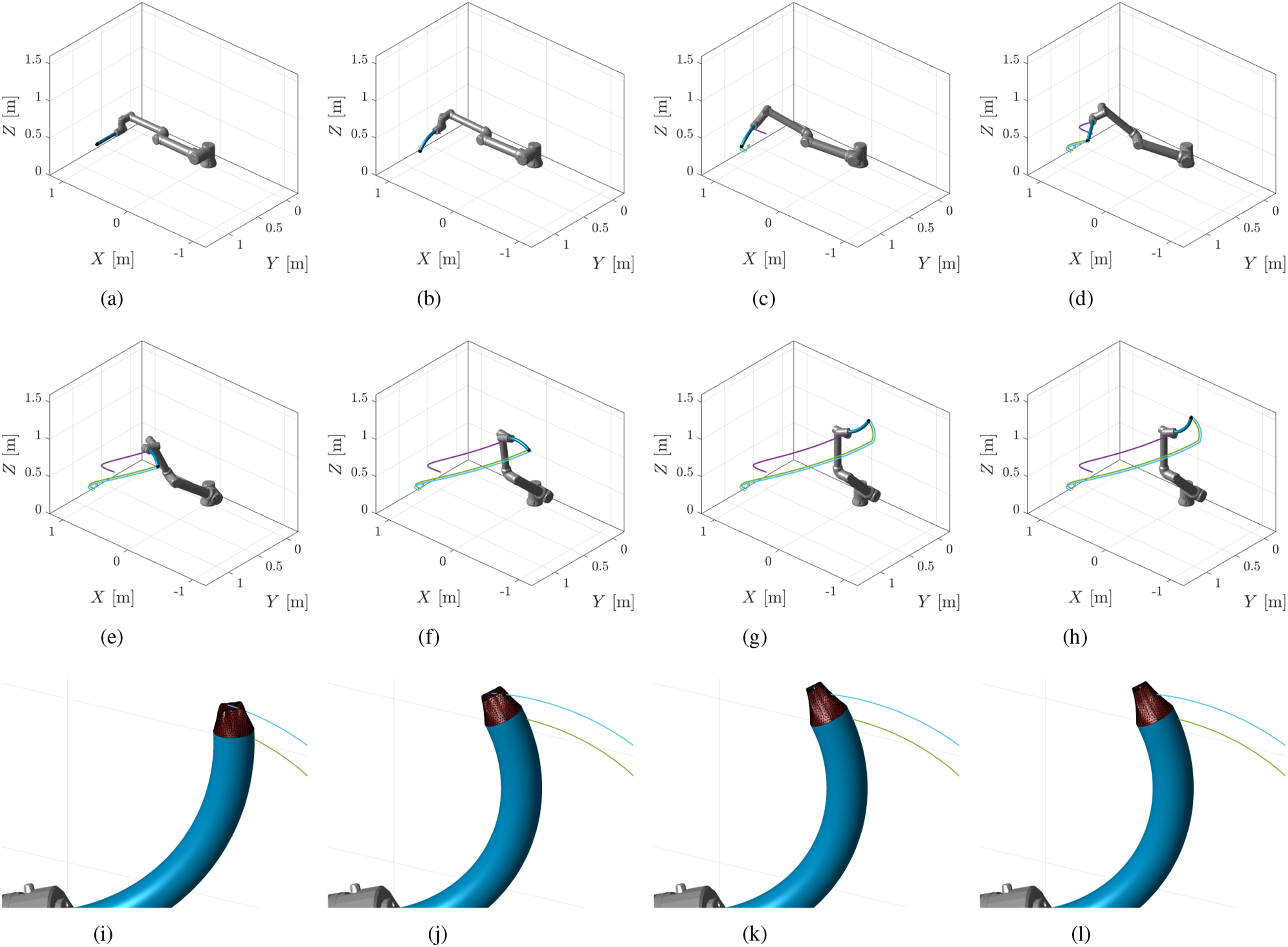
\begin{aligned} u_{GVS} & = A_{GVS}^{- 1} [K_{P_{GVS}} (q_{f_{GVS}} - q_{GVS}) - K_{D_{GVS}} \dot{q} \\ + g_{GVS} (q) + s_{GVS} (q_{GVS}, 0_{n_{GVS}})] . \end{aligned}

Also the model-based term of this controller can be implemented with a single call to the ID as ID( q , 0_n, 0_n). Finally, sub-task (iii) is solved by commanding a feedforward pressure of 2 [MPa]. We do not use any feedback controller in this case since it would require the gripper state which cannot be easily measured through proprioceptive sensors. Figure 9 shows the time evolution of the (a) configuration variables and (b) control action (note the different scale in [Pa] for the gripper input). The two feedback controllers guarantee tracking of the desired references while keeping the closed loop system provably stable. During the execution of sub-task (i), namely when the soft bodies are not actuated, the system state and input remain bounded thanks to the stability of the zero dynamics. In Figure 10, it is possible to see some snapshots of the robot motion in its workspace together with the trajectories of the distal ends of the UR10e, soft arm and gripper.

7.3. Simulation 3

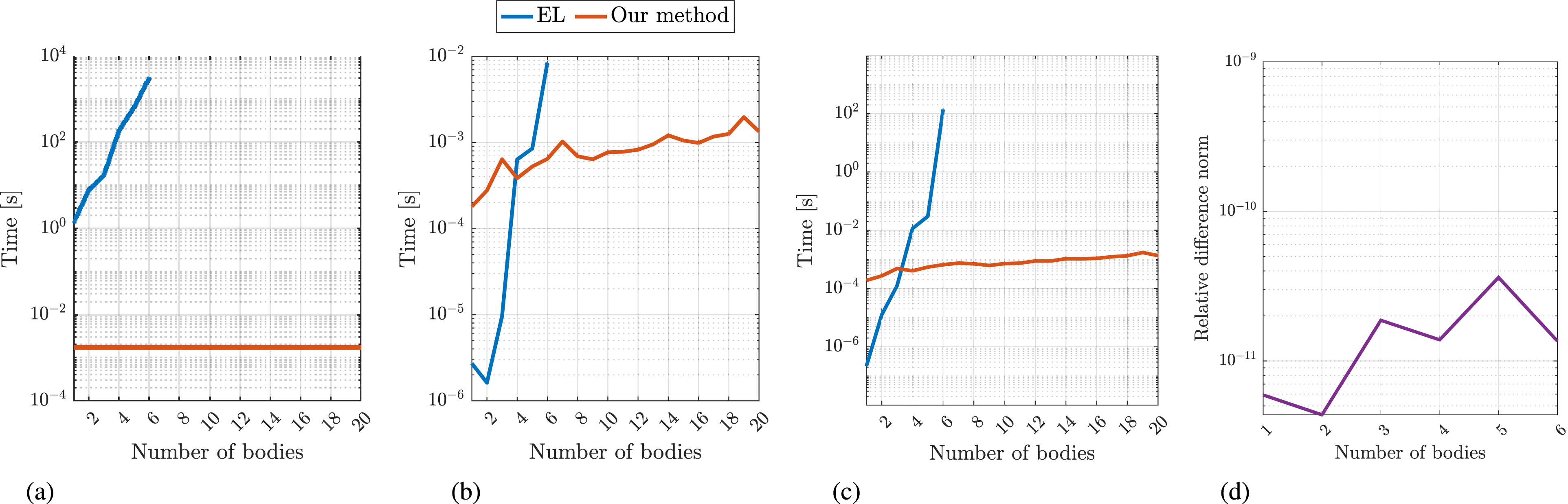
In this last simulation, we compare the computation time needed to evaluate the inertial and centrifugal generalized forces, that is, $M (q) \ddot{q}$ and $c (q, \dot{q})$ , between our approach and the EL approach. The goal of this simulation is to demonstrate the scalability of a recursive formulation of the dynamics compared to an energetic one. We use models of planar Piecewise Constant Curvature (PCC) continuum soft robots because, within a small number of bodies, the EL equations can still be computed symbolically. As shown through the toy example, also the terms appearing in our algorithm can be computed exactly for such class of robots. This implies that the computation of the dynamics with the ID algorithm remains exact independent of the number of bodies. Note that we do not compare our method with specific implementations for discrete Cosserat rods (Caasenbrood et al., 2024; Mathew et al., 2022) for two main reasons. First, the EL approach is the only method available for computing the ID for the class of soft robots considered in this paper. Second, a fair comparison would require using the same programming language and implementation by the same person, as performance can vary significantly due to these factors. In addition, we do not claim that our algorithms are more efficient than specific implementations for soft robot subclasses. On the other hand, as shown in the previous simulations, we can solve the ID problem not only for discrete Cosserat rods but also for more generic soft robot models.

By using Algorithm 1, the inertial and centrifugal forces are computed with the following arguments

M (q) \ddot{q} = I I D (q, 0_{n}, \ddot{q}),

and

c (q, \dot{q}) = I I D (q, \dot{q}, 0_{n}) .

In contrast, the evaluation of the above terms using the EL formulation involves computing the Lagrangian symbolically with the moving frame algorithm. The inertial and centrifugal forces are then obtained through symbolic differentiation. These expressions are simplified and exported as MATLAB functions for numerical evaluation.

We compare the two approaches by measuring the time needed to build the model, and evaluate $M (q) \ddot{q}$ and $c (q, \dot{q})$ through multiple calls of the corresponding methods, subsequently calculating the median and standard deviation of these measurements. The bodies have radius 0.03 [m], rest length 0.3 [m], and mass density 1000 [kg m⁻³]. Figure 11(a)–11(c) shows the simulation outcomes for unitary values of the configuration variables and their time derivatives. Using the EL equations, we could compute the model for only up to six bodies. After this number, the computation time exploded and it became impractical to obtain the dynamics. Instead, for our approach, the time to build the model remains below 4.52 [s] up to twenty bodies (see Figure 11(a)) as it is just the time needed to compute the functional expression of the integrals from the kinematics and allocate in memory the objects representing the bodies. When the number of bodies is small, the EL method is faster because it provides a closed-form expression of the generalized forces. However, the computation time increases exponentially (note the logarithmic scale) and quickly explodes. On the other hand, once the local body kinematics is updated, our algorithm computes the terms iteratively by performing algebraic operations, the most of which have dimension three. Indeed, recall that $M_{i}$ depends on three-dimensional vectors. Furthermore, memory efficiency is enhanced by coding the functional expression of integrals and partial derivatives only once for all bodies. Figure 11(d) shows the norm of the difference in the evaluation of the ID between the two approaches. Specifically, for each model, we evaluate the ID using the EL method and our algorithm with hundred random samples of triplets $(q, \dot{q}, \ddot{q})$ ranging in the intervals [ q _min, q _max] = [−π, π] [rad], $[{\dot{q}}_{\min}, {\dot{q}}_{\max}] = [- 10,10] [r a d s^{- 1}]$ and $[{\ddot{q}}_{\min}, {\ddot{q}}_{\max}] = [- 100,100] [r a d s^{- 2}]$ . Then, we compute the relative difference between the outputs and subsequently the mean and standard deviation.

8. Conclusions and future work

This paper presents a recursive formulation of the equations of motion for holonomically constrained serial soft robotic systems whose kinematics can described or approximated by a finite number of configuration variables. The approach is independent of the body kinematics, domain, and type. However, since the kinematics is treated as a black box function, recursivity can be developed only between the bodies of the system and not within the material domain.

By considering a generic kinematic model for each soft body, the equations of motion are derived using the weak form of dynamics and the Kane method. It is then proven that these equations admit a recursive expression, enabling the development of algorithms solving the inverse dynamics problem. The procedure has linear complexity in the number of bodies, or equivalently in the number of degrees of freedom, making it optimal. Additionally, it is demonstrated that it is possible to simultaneously evaluate the mass matrix and inverse dynamics without affecting computational complexity.

The versatility of the method is shown through simulations of a new reduced-order model of a trimmed helicoid robot and a hybrid arm consisting of rigid and soft bodies with different kinematic models. Its scalability is also illustrated in a comparison with the Euler–Lagrange method, which is the only approach that allows the computation of the inverse dynamics for the considered class of robots.

Future work will focus on the experimental validation of the method for model-based control. Additionally, we aim to investigate the modifications needed for the algorithm to handle non-holonomic constraints. Another research direction is to explore the recursive form of the dynamics to optimally solve the forward dynamics problem.

Supplemental Material

Supplemental Material - Recursive model-agnostic inverse dynamics of serial soft-rigid robots

Supplemental Material for Recursive model-agnostic inverse dynamics of serial soft-rigid robots by Pietro Pustina, Cosimo Della Santina, and Alessandro De Luca in The International Journal of Robotics Research

Footnotes

Declaration of conflicting interests

The author(s) declared no potential conflicts of interest with respect to the research, authorship, and/or publication of this article.

Funding

The author(s) disclosed receipt of the following financial support for the research, authorship, and/or publication of this article: This work was partly supported by PNRR MUR project PE0000013-FAIR.

ORCID iDs

Pietro Pustina

Cosimo Della Santina

Alessandro De Luca

Supplemental Material

Supplemental material for this article is available online.

Notes

Appendix

References

Abraham

Marsden

Tudor

(2016) Manifolds, Tensor Analysis, and Applications. Springer New York.

Amirouche

FML

Xie

(1993) An explicit matrix formulation of the dynamical equations for flexible multibody systems: a recursive approach. Computers & Structures 46(2): 311–321.

Armanini

Boyer

Mathew

, et al. (2023) Soft robots modeling: A structured overview. IEEE Transactions on Robotics 39(3): 1728–1748.

Banerjee

(2022) Flexible Multibody Dynamics: Efficient Formulations with Applications. 2nd edition. CRC Press.

Banerjee

Dickens

(1990) Dynamics of an arbitrary flexible body in large rotation and translation. Journal of Guidance, Control, and Dynamics 13(2): 221–227.

Bevilacqua

Soleti

Naso

, et al. (2022) Bio-inspired flapping wing antagonist actuation with SMA wires. Proc. Int. Conf. and Exhibition on New Actuator Systems and Applications. 1–4.

Book

(1984) Recursive Lagrangian dynamics of flexible manipulator arms. The International Journal of Robotics Research 3(3): 87–101.

Boyer

Khalil

(1998) An efficient calculation of flexible manipulator inverse dynamics. The International Journal of Robotics Research 17(3): 282–293.

Boyer

Lebastard

Candelier

, et al. (2020) Dynamics of continuum and soft robots: A strain parameterization based approach. IEEE Transactions on Robotics 37(3): 847–863.

10.

Boyer

Gotelli

Tempel

, et al. (2024) Implicit time-integration simulation of robots with rigid bodies and Cosserat rods based on a Newton–Euler recursive algorithm. IEEE Transactions on Robotics 40: 677–696.

11.

Bruder

Gillespie

, et al. (2021) Data-driven control of soft robots using Koopman operator theory. IEEE Transactions on Robotics 37(3): 948–961.

12.

Buondonno

De Luca

(2016) Efficient computation of inverse dynamics and feedback linearization for VSA-based robots. IEEE Robotics and Automation Letters 1(2): 908–915.

13.

Caasenbrood

Pogromsky

Nijmeijer

(2023) Control-oriented models for hyperelastic soft robots through differential geometry of curves. Soft Robotics 10(1): 129–148.

14.

Caasenbrood

Pogromsky

Nijmeijer

(2024) Sorotoki: A MATLAB toolkit for design, modeling, and control of soft robots. IEEE Access 12: 17604–17638.

15.

Chang

Halder

Shih

, et al. (2023) Energy-shaping control of a muscular octopus arm moving in three dimensions. Proc. of the Royal Society A 479(2270): 20220593.

16.

Chen

(2001) Dynamic modeling of multi-link flexible robotic manipulators. Computers & Structures 79(2): 183–195.

17.

Chen

Wang

(2020) Design optimization of soft robots: A review of the state of the art. IEEE Robotics and Automation Magazine 27(4): 27–43.

18.

Coevoet

Morales-Bieze

Largilliere

, et al. (2017) Software toolkit for modeling, simulation, and control of soft robots. Advanced Robotics 31(22): 1208–1224.

19.

Davis

Rabinowitz

(2007) Methods of Numerical Integration. Courier Corporation.

20.

De Luca

Book

(2016) Robots with flexible elements. In: Siciliano

Khatib

(eds) Springer Handbook of Robotics. 2nd edition. Springer, 243–282.

21.

Della Santina

Albu-Schaeffer

(2020) Exciting efficient oscillations in nonlinear mechanical systems through eigenmanifold stabilization. IEEE Control Systems Letters 5(6): 1916–1921.

22.

Della Santina

Katzschmann

Bicchi

, et al. (2020b) Model-based dynamic feedback control of a planar soft robot: Trajectory tracking and interaction with the environment. The International Journal of Robotics Research 39(4): 490–513.

23.

Della Santina

Rus

(2019) Control oriented modeling of soft tobots: The polynomial curvature case. IEEE Robotics and Automation Letters 5(2): 290–298.

24.

Della Santina

Bicchi

Rus

(2019) Dynamic control of soft robots with internal constraints in the presence of obstacles. Proc. IEEE/RSJ Int. Conf. on Intelligent Robots and Systems. 6622–6629.

25.

Della Santina

Catalano

Bicchi

(2020a) Soft robots. In: Ang

Khatib

Siciliano

(eds) Encyclopedia of Robotics. Springer, 1–15.

26.

Della Santina

Duriez

Rus

(2023) Model-based control of soft robots: A survey of the state of the art and open challenges. IEEE Control Systems Magazine 43(3): 30–65.

27.

Dinev

Liu

, et al. (2018) FEPR: Fast energy projection for real-time simulation of deformable objects. ACM Transactions on Graphics 37(4): 1–12.

28.

Dubied

Michelis

Spielberg

, et al. (2022) Sim-to-real for soft robots using differentiable FEM: Recipes for meshing, damping, and actuation. IEEE Robotics and Automation Letters 7(2): 5015–5022.

29.

Featherstone

(2014) Rigid Body Dynamics Algorithms. Springer.

30.

Ferrentino

Roels

Brancart

, et al. (2023) Finite element analysis-based soft robotic modeling: Simulating a soft actuator in SOFA. IEEE Robotics and Automation Magazine 31(3): 97–105.

31.

Ferrolho

Ivan

Merkt

, et al. (2021) Inverse dynamics vs. forward dynamics in direct transcription formulations for trajectory optimization. Proc. IEEE Int. Conf. on Robotics and Automation. 12752–12758.

32.

Gaz

Cognetti

Oliva

, et al. (2019) Dynamic identification of the Franka Emika Panda robot with retrieval of feasible parameters using penalty-based optimization. IEEE Robotics and Automation Letters 4(4): 4147–4154.

33.

Godage

Webster

Walker

(2019) Center-of-gravity-based approach for modeling dynamics of multisection continuum arms. IEEE Transactions on Robotics 35(5): 1097–1108.

34.

Grassmann

Chen

Liang

, et al. (2022) A dataset and benchmark for learning the kinematics of concentric tube continuum robots. Proc. IEEE/RSJ Int. Conf. on Intelligent Robots and Systems. 9550–9557.

35.

Grazioso

Di Gironimo

Siciliano

(2019) A geometrically exact model for soft continuum robots: The finite element deformation space formulation. Soft Robotics 6(6): 790–811.

36.

Guan

Stella

Della Santina

, et al. (2023) Trimmed helicoids: An architectured soft structure yielding soft robots with high precision, large workspace, and compliant interactions. Npj Robotics 1: 4.

37.

Han

Liu

, et al. (2021) Distributed parameter modeling and boundary control of an octopus tentacle-inspired soft robot. IEEE Transactions on Control Systems Technology 30(3): 1244–1256.

38.

Hoeijmakers

HWM

Koerkamp

LHG

de Santana

, et al. (2022) Investigation flapping-flight aerodynamics of a robotic bird. In: Proc. 33th Congr. Int. Council of the Aeronautical Sciences, 3326–3351.

39.

Hollerbach

(1980) A recursive Lagrangian formulation of maniputator dynamics and a comparative study of dynamics formulation complexity. IEEE Transactions on Systems, Man, and Cybernetics 10(11): 730–736.

40.

Wang

Cheng

, et al. (2020) Origami spring–inspired metamaterials and robots: An attempt at fully programmable robotics. Science Progress 103(3): 0036850420946162.

41.

Jensen

Johnson

Lindberg

, et al. (2022) Tractable and intuitive dynamic model for soft robots via the recursive Newton-Euler algorithm. Proc. IEEE Int. Conf. on Soft Robotics. 416–422.

42.

Kane

Levinson

(1983) The use of Kane’s dynamical equations in robotics. The International Journal of Robotics Research 2(3): 3–21.

43.

Khalil

Boyer

Morsli

(2017) General dynamic algorithm for floating base tree structure robots with flexible joints and links. ASME Journal of Mechanisms and Robotics 9(3): 031003.

44.

Korayem

Shafei

Dehkordi

(2014) Systematic modeling of a chain of N-flexible link manipulators connected by revolute–prismatic joints using recursive Gibbs-Appell formulation. Archive of Applied Mechanics 84: 187–206.

45.

Lacarbonara

(2013) Nonlinear Structural Mechanics: Theory, Dynamical Phenomena and Modeling. Springer.

46.

Lee

Noh

Lee

, et al. (2009) Development of bio-mimetic robot hand using parallel mechanisms. Proc. IEEE Int. Conf. on Robotics and Biomimetics. 550–555.

47.

Shintake

Hayashibe

(2021) Deep reinforcement learning framework for underwater locomotion of soft robot. Proc. IEEE Int. Conf. on Robotics and Automation. 12033–12039.

48.

Wang

Kwok

(2022) Towards adaptive continuous control of soft robotic manipulator using reinforcement learning. Proc. IEEE/RSJ Int. Conf. on Intelligent Robots and Systems. 7074–7081.

49.

Donato

Lomonaco

, et al. (2024) Continual policy distillation of reinforcement learning-based controllers for soft robotic in-hand manipulation. Proc. IEEE Int. Conf. on Soft Robotics. 1026–1033.

50.

Lilly

Orin

(1990) O(N) recursive algorithm for the operational space inertia matrix of a robot manipulator. IFAC Proceedings Volumes 23(8): 275–279.

51.

Lin

Jiang

Shang

(2022) The emerging technology of biohybrid micro-robots: A review. Bio-Design and Manufacturing 5: 107–132.

52.

Liu

Bai

, et al. (2023a) Large deformation and failure analysis of the corrugated flexible composite skin for morphing wing. Engineering Structures 278: 115463.

53.

Liu

Duan

, et al. (2023b) On a hierarchical adaptive and robust inverse dynamic control strategy with experiment for robot manipulators under uncertainties. Control Engineering Practice 138: 105604.

54.

Longhini

Moletta

Reichlin

, et al. (2023) EDO-net: Learning elastic properties of deformable objects from graph dynamics. Proc. IEEE Int. Conf. on Robotics and Automation. 3875–3881.

55.

Mathew

Hmida

Armanini

, et al. (2022) SoRoSim: A MATLAB toolbox for hybrid rigid–soft robots based on the geometric variable-strain approach. IEEE Robotics and Automation Magazine 30(3): 106–122.

56.

Mathew

Feliu-Talegon

Alkayas

, et al. (2024) Reduced order modeling of hybrid soft-rigid robots using global, local, and state-dependent strain parameterization. The International Journal of Robotics Research 44(1): 129–154.

57.

Ménager

Navez

Goury

, et al. (2023) Direct and inverse modeling of soft robots by learning a condensed FEM model. Proc. IEEE Int. Conf. on Robotics and Automation. 530–536.

58.

Bien

, et al. (2019) An efficient finite element formulation of dynamics for a flexible robot with different type of joints. Mechanism and Machine Theory 134: 267–288.

59.

Pinskier

Howard

(2022) From bioinspiration to computer generation: Developments in autonomous soft robot design. Advanced Intelligent Systems 4(1): 2100086.

60.

Müller

Abdalla

, et al. (1996) Parallel computation of the inertia matrix of a tree type robot using one directional recursion of Newton-Euler formulation. Journal of Intelligent and Robotic Systems 15: 33–39.

61.

Pustina

Della Santina

De Luca

(2022) Feedback regulation of elastically decoupled underactuated soft robots. IEEE Robotics and Automation Letters 7(2): 4512–4519.

62.

Pustina

Della Santina

Boyer

, et al. (2024) Input decoupling of Lagrangian systems via coordinate transformation: General characterization and its application to soft robotics. IEEE Transactions on Robotics 40: 2098–2110.

63.

Qin

Peng

Huang

, et al. (2024) Modeling and simulation of dynamics in soft robotics: A review of numerical approaches. Current Robotics Reports 5: 1–13.

64.

Renda

Seneviratne

(2018) A geometric and unified approach for modeling soft-rigid multi-body systems with lumped and distributed degrees of freedom. Proc. IEEE Int. Conf. on Robotics and Automation. 1567–1574.

65.

Renda

Boyer

Dias

, et al. (2018) Discrete Cosserat approach for multisection soft manipulator dynamics. IEEE Transactions on Robotics 34(6): 1518–1533.

66.

Renda

Armanini

Lebastard

, et al. (2020) A geometric variable-strain approach for static modeling of soft manipulators with tendon and fluidic actuation. IEEE Robotics and Automation Letters 5(3): 4006–4013.

67.

Renda

Armanini

Mathew

, et al. (2022) Geometrically-exact inverse kinematic control of soft manipulators with general threadlike actuators’ routing. IEEE Robotics and Automation Letters 7(3): 7311–7318.

68.

Rodriguez

Kreutz-Delgado

(1992) Spatial operator factorization and inversion of the manipulator mass matrix. IEEE Transactions on Robotics and Automation 8(1): 65–76.

69.

Rone

Ben-Tzvi

(2013) Continuum robot dynamics utilizing the principle of virtual power. IEEE Transactions on Robotics 30(1): 275–287.

70.

Rus

Tolley

(2015) Design, fabrication and control of soft robots. Nature 521(7553): 467–475.

71.

Russo

Sadati

SMH

Dong

, et al. (2023) Continuum robots: An overview. Advanced Intelligent Systems 5(5): 2200367.

72.

Sadati

Naghibi

Walker

, et al. (2017) Control space reduction and real-time accurate modeling of continuum manipulators using Ritz and Ritz–Galerkin methods. IEEE Robotics and Automation Letters 3(1): 328–335.

73.

Sadati

Naghibi

Da Cruz

, et al. (2020) Reduced-order modeling and model order reduction for soft robots. ResearchGate Preprint. DOI: 10.13140/RG.2.2.24115.86568.

74.

Sadati

Naghibi

Shiva

, et al. (2021) TMTDyn: A Matlab package for modeling and control of hybrid rigid–continuum robots based on discretized lumped systems and reduced-order models. The International Journal of Robotics Research 40(1): 296–347.

75.

Santibañez

Kelly

(2001) PD control with feedforward compensation for robot manipulators: Analysis and experimentation. Robotica 19(1): 11–19.

76.

Saunders

Trimmer

Rife

(2010) Modeling locomotion of a soft-bodied arthropod using inverse dynamics. Bioinspiration & Biomimetics 6(1): 016001.

77.

Sfakiotakis

Kazakidi

Chatzidaki

, et al. (2014) Multi-arm robotic swimming with octopus-inspired compliant web. Proc. IEEE/RSJ Int. Conf. on Intelligent Robots and Systems. 302–308.

78.

Shabana

(1990) Dynamics of flexible bodies using generalized Newton-Euler equations. ASME Journal of Dynamic Systems, Measurement, and Control 112(3): 496–503.

79.

Sharp

Romero

Jacobson

, et al. (2023) Data-free learning of reduced-order kinematics. In: Proc. ACM SIGGRAPH, 1–9.

80.

Singh

VanderVoort

Likins

(1985) Dynamics of flexible bodies in tree topology — a computer-oriented approach. Journal of Guidance, Control, and Dynamics 8(5): 584–590.

81.

Spong

(1994) Partial feedback linearization of underactuated mechanical systems. Proc. IEEE Int. Conf. on Intelligent Robots and Systems. 314–321.

82.

Stramigioli

(2024) The principal bundle structure of continuum mechanics. Journal of Geometry and Physics 200: 105172.

83.

Sun

Chen

, et al. (2020) Biohybrid robotics with living cell actuation. Chemical Society Reviews 49(12): 4043–4069.

84.

Tiburzio

Coleman

Della Santina

(2024) Model-based manipulation of deformable objects with non-negligible dynamics as shape regulation. arXiv:2402: 16114.

85.

Tonkens

Lorenzetti

Pavone

(2021) Soft robot optimal control via reduced order finite element models. Proc. IEEE Int. Conf. on Robotics and Automation. 12010–12016.

86.

Wang

Chan

Yuan

, et al. (2021) Endoscopy-assisted magnetic navigation of biohybrid soft microrobots with rapid endoluminal delivery and imaging. Science Robotics 6(52): eabd2813.

87.

Webster

III RJ

Jones

(2010) Design and kinematic modeling of constant curvature continuum robots: A review. The International Journal of Robotics Research 29(13): 1661–1683.

88.

Whittaker

(1964) A Treatise on the Analytical Dynamics of Particles and Rigid Bodies. CUP Archive.

89.

Wotte

Dummer

Botteghi

, et al. (2023) Discovering efficient periodic behaviors in mechanical systems via neural approximators. Optimal Control Applications and Methods 44(6): 3052–3079.

90.

Chirikjian

(2023) Model reduction in soft robotics using locally volume-preserving primitives. IEEE Robotics and Automation Letters 8(9): 5831–5838.

91.

Yin

Varava

Kragic

(2021) Modeling, learning, perception, and control methods for deformable object manipulation. Science Robotics 6(54): eabd8803.

92.

Zhang

(2009) Recursive Lagrangian dynamic modeling and simulation of multi-link spatial flexible manipulator arms. Applied Mathematics and Mechanics 30(10): 1283–1294.

93.

Zheng

Lin

(2022) PDE-based dynamic control and estimation of soft robotic arms. Proc. IEEE Conf. on Decision and Control. 2702–2707.

94.

Zhu

Cherubini

Dune

, et al. (2022) Challenges and outlook in robotic manipulation of deformable objects. IEEE Robotics and Automation Magazine 29(3): 67–77.

Supplementary Material

Please find the following supplemental material available below.

For Open Access articles published under a Creative Commons License, all supplemental material carries the same license as the article it is associated with.

For non-Open Access articles published, all supplemental material carries a non-exclusive license, and permission requests for re-use of supplemental material or any part of supplemental material shall be sent directly to the copyright owner as specified in the copyright notice associated with the article.

0.00 MB

4.53 MB