
Abstract
Consistent maps are key for most autonomous mobile robots, and they often use SLAM approaches to build such maps. Loop closures via place recognition help to maintain accurate pose estimates by mitigating global drift, and are thus key for realizing an effective SLAM system. This paper presents a robust loop closure detection pipeline for outdoor SLAM with LiDAR-equipped robots. Our method handles various LiDAR sensors with different scanning patterns, fields of view, and resolutions. It generates local maps from LiDAR scans and aligns them using a ground alignment module to handle both planar and non-planar motion of the LiDAR, ensuring applicability across platforms. The method uses density-preserving bird’s-eye-view projections of these local maps and extracts ORB feature descriptors for place recognition. It stores the feature descriptors in a binary search tree for efficient retrieval, and self-similarity pruning addresses perceptual aliasing in repetitive environments. Extensive experiments on public and self-recorded datasets demonstrate accurate loop closure detection, long-term localization, and cross-platform multi-map alignment, agnostic to the LiDAR scanning patterns, fields of view, and motion profiles. We provide the code for our pipeline as open-source software at https://github.com/PRBonn/MapClosures.
1. Introduction
Mobile robots must navigate their surroundings safely and efficiently. They need to know their location within the environment to successfully navigate to a desired place or explore new areas. Accurate ego-motion estimation helps robots generate accurate maps of the environment, which they can use for navigation. Traditionally, robots often localize themselves using data acquired through exteroceptive sensors like cameras and laser range sensors (LiDAR), proprioceptive sensors like wheel odometers and IMUs, or a combination. Depending on the application and availability, outdoor systems often also exploit GNSS for global positioning.
LiDAR sensors are frequently used in robotics due to their accurate and dense 3D range data. Many previous studies have advanced the field of sequential pose estimation using LiDAR sensors (Dellenbach et al., 2022; Ferrari et al., 2024; Fontana et al., 2016; Guadagnino et al., 2022; Vizzo et al., 2023). Such sequential pose estimation alone, also called sensor odometry, suffers from drifting pose estimates over time due to inherent noise in the robot motion and sensor data, dynamics in the environment, and non-trivial data association problems.
We can compensate for such drift and improve pose estimation by recognizing places previously visited by the robot. This task is referred to as loop closing. It allows the use of geometric information from the LiDAR observations at revisited locations to correct the pose drift, for example, through pose-graph optimization. Robust loop closure detection is paramount in simultaneous localization and mapping (SLAM) systems. Robots must recognize that they have returned to a previously visited place to close a loop.
Place recognition is a key sub-task within loop closure detection, which performs data associations between the robot’s current view and a database of previously seen places. Generating a database of places is a non-trivial task that requires crafting an as unique as possible description of the environment, invariant to changes in viewpoint. Also, such a database should filter dynamic objects appearing in the sensor data to achieve robust place recognition across long time intervals. Perceptual aliasing is another challenge, as distinct places with similar structures can confuse place recognition algorithms. This could lead to false-positive loop closures that can adversely impact global SLAM estimates (Bailey and Durrant-Whyte, 2006; Blanco et al., 2013; Ramos et al., 2007). Furthermore, to perform place recognition for loop closing in a SLAM system, the database should encode the scene’s geometry to allow for relative pose estimation between different revisit viewpoints for the pose-graph optimization.
Global feature descriptors computed over the entire point clouds are easy to store in a database and allow for quick retrieval of revisit candidates (Kim et al., 2021; Lu et al., 2022; Luo et al., 2025; Uy and Lee, 2018; Xu et al., 2023). However, such methods often do not provide an initial geometric alignment between the detected loop closures and require an additional point cloud registration step to perform such an alignment. In contrast, feature descriptors computed over local 3D patches within a point cloud can aid the geometric alignment of revisited locations (Blanco et al., 2013; Steder et al., 2011; Yang et al., 2017). However, they require a nuanced approach to store the feature descriptors efficiently in a database.
Due to the algorithmic complexity of processing 3D point clouds to obtain local or global feature descriptors, several methods perform a bird’s-eye-view (BEV) projection (Kim et al., 2021; Li and Li, 2021; Luo et al., 2023) or a cylindrical projection (Chen et al., 2020; Ma et al., 2022; Steder et al., 2010) of the point clouds. This results in a 2D representation of the point cloud data, allowing faster feature detection and matching for online loop closure detection in SLAM.
The main contribution of this article is a robust loop closure detection pipeline that works with various LiDAR sensors having different motion profiles, invariant to their scanning pattern, field of view (FoV), and resolution. We generate local maps by aggregating consecutive scans and creating a density-preserving BEV projection of the local maps as an intermediate 2D representation for computing local features describing the structural information in the 3D local maps. Since the ground planes can be consistently identified in outdoor environments during revisits, we use them as a reference plane to ensure consistent BEV projections across revisits. We propose a ground alignment module to identify such a ground plane in each local map and transform the local map such that this ground plane coincides with the local xy-plane of the reference frame. This simplifies the BEV projection and restricts the loop closure alignment to two dimensions on the common ground plane and makes our approach applicable to various motion profiles of LiDAR sensors. We store binary ORB feature descriptors from the BEV projection into a Hamming distance embedding binary search tree (HBST). We design our approach to be robust against the effects of scene similarity, also known as perceptual aliasing, by performing a self-similarity pruning of the feature descriptors before inserting them in the database. Using a Hamming distance metric, we obtain loop closure candidates by matching feature descriptors from query local maps against this database. Our subsequent random sample consensus (RANSAC) based geometric validation step provides loop closures along with a 2D alignment between BEV projections of the local maps. When combined with the ground alignment estimate of each local map, we obtain a complete 3D estimate of the global alignment between the local maps. We provide an extensive experimental evaluation on multiple datasets, with sequences recorded with a wide range of LiDAR sensors mounted on different mobile platforms, testing the accuracy and robustness of our pipeline in challenging scenarios.
In sum, we make six key claims, which we support with the paper and our experimental evaluation. Our approach (1) Detects loop closures between local maps generated from various LiDAR sensors with different scanning patterns, FoVs, and resolutions; (2) Performs multi-session loop closure detection and alignment with long-term revisits; (3) Works with handheld platforms having non-planar motion in the LiDAR sensor frame; (4) Is robust against perceptual aliasing in environments with repetitive structures; (5) Provides a complete 3D rigid-body transform to align the detected loop closures; (6) Detects loop closures between sequences having minimal overlap, recorded with different LiDAR sensor platforms, enabling cross-platform multi-map alignment.
This article extends our previous conference paper (Gupta et al., 2024), which proposed loop closure detection using local maps by detecting local feature descriptors from their BEV projections and generating a binary search tree database. It extends the earlier work in the following critical ways: (1) relaxation of the planar-motion assumption through a new ground alignment module; (2) a complete 3D alignment estimate of the detected loop closures; (3) a pruning strategy on the ORB feature descriptors computed from the BEV density images to mitigate the issues with perceptual aliasing; (4) an extensive experimental evaluation on multiple datasets, with sequences recorded with a wide range of LiDAR sensors mounted on different mobile platforms, testing the accuracy and robustness of our pipeline in challenging scenarios.
The open-source implementation of our previous approach and the proposed approach are available at https://github.com/PRBonn/MapClosures.
2. Related work
Zhang et al. (2024) provide a thorough literature review on place recognition for loop closures in 3D LiDAR SLAM and Yin et al. (2024) on LiDAR-based global localization. This section briefly overviews key approaches for LiDAR-based loop closure detection in SLAM.
The most straightforward approach to loop closure detection in SLAM is using the individual scans and their poses obtained from odometry. The similarity of poses between non-consecutive scans within a search radius is used to detect loop closures (Rottmann et al., 2019; Shan et al., 2020). S4-SLAM (Zhou et al., 2021) and the approach by Mendes et al. (2016) use the odometry information to compute the overlap between point clouds to check if they are recorded from the same location. Chen et al. (2020) use convolutional neural networks to calculate the overlap between the range image representations of point clouds to detect loops. These methods primarily perform a place retrieval task, often requiring a subsequent point cloud registration step to validate the loop closures. Furthermore, they can be sensitive to the magnitude of drift present in the odometry pose estimates, requiring a search radius proportional to the drift.
2.1. Methods using 3D features from point clouds
Place recognition has been widely studied in the context of camera images (Cummins and Newman, 2008; Galvez-Lopez and Tardos, 2012; Mur-Artal et al., 2015; Vysotska and Stachniss, 2016, 2019). Consequently, much research on LiDAR place recognition for loop closing has been motivated by approaches in the camera vision domain. In particular, many approaches have extended the idea of local feature descriptors to 3D point clouds (Johnson and Hebert, 1999; Rusu et al., 2009; Salti et al., 2014), discretizing the neighborhood around 3D features into a geometrical grid. They compute a descriptor from the points in this neighborhood based on their height (Bosse and Zlot, 2013), density (Frome et al., 2004; Tombari et al., 2010), or distance and angle (Rusu et al., 2008). These local feature descriptor-based methods estimate a complete 3D relative pose between the loop closures. However, they have a high computational cost to identify such feature descriptors from 3D point clouds. They are sensitive to the radially increasing sparsity of point clouds obtained from a standard spinning LiDAR.
Several methods (Kim et al., 2024; Magnusson et al., 2009; Röhling et al., 2015; Uy and Lee, 2018) take an orthogonal approach by computing one global descriptor per LiDAR scan. Magnusson et al. (2009) superimpose a voxel grid on the point clouds and approximate a normal distribution over points in each grid cell. They compute a global descriptor for the point clouds by computing a histogram over these normal distributions. More recently, Kim et al. (2024) proposed a lightweight global descriptor with SOLiD by representing point clouds in polar coordinates and discretizing them into range-elevation and azimuth-elevation directions, respectively, with each discrete bin storing the number of points. Such global descriptors are easy to store in a simple database, resulting in a faster matching process to retrieve loop closure candidates. However, global descriptor-based methods typically require revisits within small error margins around the reference pose to limit the variation in the global descriptor. They often do not generalize when detecting loop closures across LiDARs with different scanning patterns and resolutions.
2.2. Two-dimensional projection-based methods
Many recent works focus on speeding up the recognition by describing 3D point clouds by a 2D projection (Kim and Kim, 2018; Li and Li, 2021; Luo et al., 2023; Xu et al., 2023; Yuan et al., 2024). Even though such a projection results in loss of geometric information, these methods perform comparably and sometimes even better than their full 3D counterparts, especially in outdoor scenes. Among the two-dimensional projection-based methods, the cylindrical projection into range images (Chen et al., 2020; Shan et al., 2021; Steder et al., 2010, 2011) and the orthogonal projection into BEV images (Kim et al., 2021; Lu et al., 2022; Luo et al., 2021; Wang et al., 2020; Yuan et al., 2023) are widely used 2D projections.
Range image projections are equivariant to azimuthal rotations due to the underlying cylindrical projection. They can recover the relative yaw between loop closures but suffer from scale distortions due to lateral shifts in the LiDAR viewpoint. On the other hand, BEV projections preserve 2D geometry along the local ground plane, which is vital for autonomous ground robots. Among the BEV projection methods, the elevation map is widely used (Kim et al., 2021; Kim and Kim, 2018; Luo et al., 2023; Yuan et al., 2023). An elevation map preserves the maximum elevation within each discrete pillar in the BEV representation.
Scan Context by Kim and Kim (2018) is a popular LiDAR-based loop closure approach. It computes a global descriptor for each LiDAR scan using the elevation map in polar coordinates. The polar coordinates make the descriptor equivariant to in-plane rotations, thereby allowing the loop closure alignment module to estimate the relative yaw between LiDAR scans from the same location. However, the polar coordinate representation can be sensitive to in-plane translations. Scan Context++ (Kim et al., 2021) improves upon this drawback of Scan Context and computes elevation maps in Cartesian coordinates to augment the polar elevation maps. However, preserving the maximum elevation of the points after the BEV projection makes the two approaches sensitive to the vertical resolution and FoV of the LiDAR.
In contrast, BVMatch (Luo et al., 2021) proposes a density-preserving BEV projection of point clouds and a Log Gabor filtering step. It requires training a bag-of-words model to retrieve loop closure candidates, making it less suitable for real-time applications such as SLAM. Our approach also uses a density-preserving BEV projection. It generates a database of local feature descriptors from the BEV image online using the HBST data structure (Schlegel and Grisetti, 2018) for efficient operation. The use of local feature descriptors for loop closure detection has also been previously explored in the 2D LiDAR domain with traditional occupancy grid maps (Blanco et al., 2013).
Yuan et al. (2023) propose utilizing a set of geometric primitives, that is, triangles with unique side lengths, to describe a point cloud. They obtain the feature vertices of such triangles by a local BEV projection of points within voxels that lie at the boundaries of large planar regions in the environment. BTC (Yuan et al., 2024) improves upon this work by proposing a binary descriptor for a detailed representation of local geometry. They combine the triangle descriptors and the newly proposed binary descriptors to perform loop closure retrieval. The works by Yuan et al. (2023, 2024) use a local map representation of the environment by accumulating a fixed number of consecutive scans. This helps them tackle the sparsity issue present with rotating 3D LiDAR. The local maps also make their approach generalizable to LiDAR sensors with non-repetitive scanning patterns and small FoVs. We also use a local map representation to detect loop closures. However, unlike STD and BTC, we accumulate scans until a minimum displacement of the platform to ensure that the local maps capture a sufficient portion of the scene.
2.3. Learning-based approaches
The recent popularity of deep neural networks, attributed to the widespread availability of specialized hardware and software to train such networks, has generated much interest from a LiDAR-based loop closing perspective (Chen et al., 2020; Dubé et al., 2018; Komorowski, 2021; Ma et al., 2022; Ma et al. 2024). PointNet (Qi et al., 2017b) and PointNet++ (Qi et al., 2017a) use multi-layer perceptron networks to detect local feature descriptors from point clouds. PointNetVLAD (Uy and Lee, 2018) proposes an end-to-end trained neural network that combines the local feature descriptors obtained from PointNet into a global descriptor using NetVLAD (Arandjelovic et al., 2016). SegMap (Dubé et al., 2018) segments point clouds using a region-growing algorithm and computes data-driven descriptors of these segments to detect loop closures.
BEV projections are also popular with learning-based approaches (Kim et al., 2019; Luo et al., 2023, 2025; Xu et al., 2021b). Kim et al. (2019) repurpose the Scan Context (Kim and Kim, 2018) image as a three-channel image using a jet colormap over a range of structural heights. They train a convolutional neural network using these Scan Context images and perform localization as a classification task. Xu et al. (2021b) propose an encoder-decoder network to extract descriptors from differentiable Scan Context images.
Vidanapathirana et al. (2022) use a global descriptor obtained from a sparse convolutional neural network to perform loop closures. They propose a local-consistency loss to train their approach to obtain consistent local features across revisits, which they later combine into a global descriptor using a pooling and normalization strategy.
BEVPlace (Luo et al., 2023) applies group convolutions corresponding to the
Recently, Ramezani et al. (2024) proposed a place recognition method based on an attentional graph neural network representation. Their approach leverages the topological relationships between consecutive LiDAR scans within a pose-graph SLAM system by generating sub-graphs according to a travel distance criterion. They use a multi-layer perceptron to encode the odometry poses and global descriptor associated with every scan within each of the sub-graphs. For a candidate pair of sub-graphs, they construct a fully connected multiplex graph from the encoded nodes and process it through an attentional graph neural network, P-GAT, to perform place recognition.
Even though learning-based approaches achieve impressive performance regarding loop closure precision and recall metrics, they typically require a computationally expensive offline pre-training step on a GPU, affecting their application to real-time loop closure detection in SLAM.
Our method also exploits the spatio-temporal information across consecutive LiDAR scans by constructing local maps as the primary representation for loop closure detection, rather than relying on individual scans. Following our earlier work (Gupta et al., 2024), we generate local maps based on a travel displacement criteria, in contrast to Yuan et al. (2023, 2024), who accumulate a fixed number of scans. This strategy helps us overcome the sparsity of rotating LiDAR and make our method agnostic to the LiDAR sensor’s scanning pattern, FoV, and resolution. We use a density-preserving BEV projection of the local maps on the local ground plane to reduce dimensionality for computational efficiency. Subsequently, we compute ORB feature descriptors (Rublee et al., 2011) from the BEV density images and store them in an HBST database (Schlegel and Grisetti, 2018) for place recognition. We mitigate the negative impact of perceptual aliasing on our feature descriptor-matching algorithm by performing a self-similarity pruning of the ORB feature descriptors (Bosse et al., 2004). Our loop closure pipeline provides a complete 3D global alignment between the local maps.
3. Our methodology
We propose an approach to detect loop closures between local maps using their BEV representation that works with both vehicle-mounted and handheld LiDAR sensor platforms. It also provides a complete 3D initial guess of the relative pose between local maps involved in the loop closures. We present an overview of our pipeline in Figure 1. Overview of our pipeline for loop closure detection and alignment. Given a local map 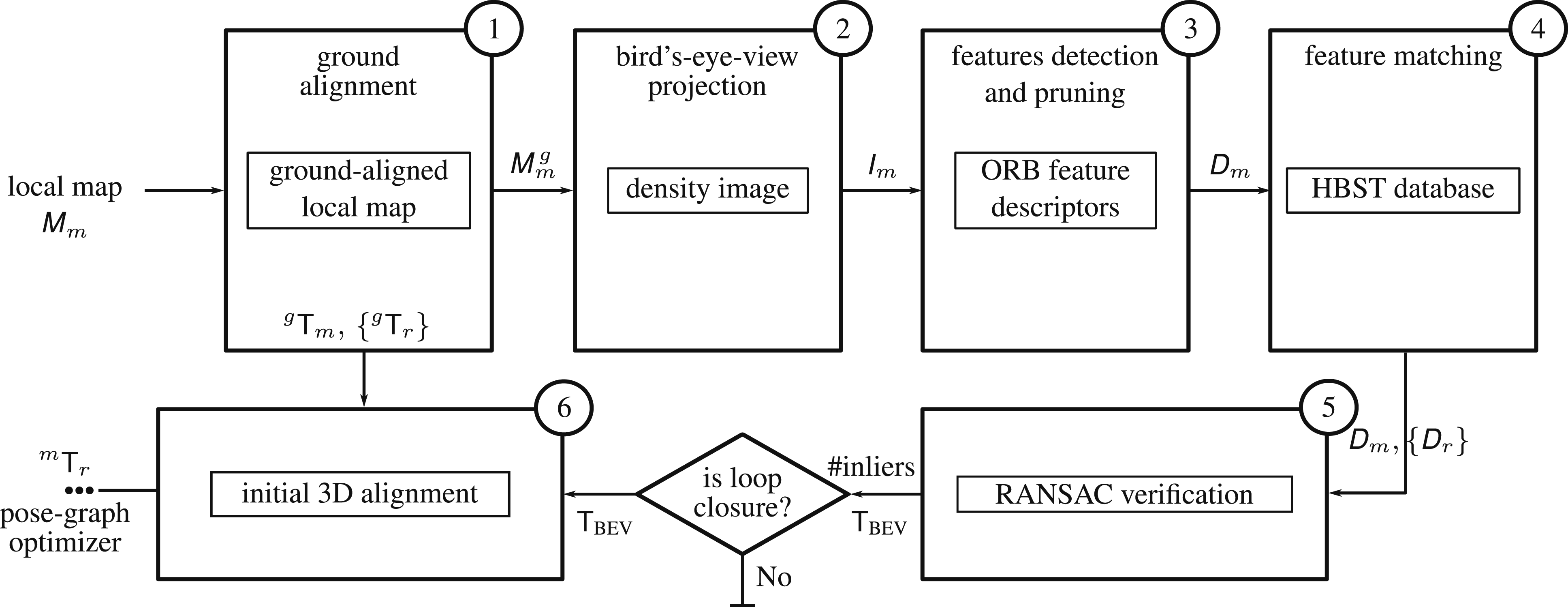
We explain in Section 3.1 the procedure to generate local maps from LiDAR point clouds based on a travel displacement criterion. Then, in Section 3.2, we present an approach to detect and align the ground plane in the local maps to the xy-plane of the local reference frame. This allows us to compute a BEV representation even in scenarios with a non-planar motion of the LiDAR sensor, as explained in Section 3.3. We compute binary descriptors for point features on these BEV images, as presented in Section 3.4. To enable place recognition using these binary feature descriptors, we store them in an HBST database (Schlegel and Grisetti, 2018) for subsequent matching with query local maps as presented in Section 3.5. We obtain a set of candidate loop closures for new feature descriptors from a query local map by matching these feature descriptors to the database. We perform loop closure validation and geometric alignment in 2D between the matched feature descriptors using a RANSAC (Fischler and Bolles, 1981) scheme described in Section 3.6. This 2D alignment, together with the ground alignment for each local map, provides the relative 3D transform aligning each pair of loop-closed local maps.
3.1. Creation of local maps
Our approach uses local point cloud maps of the environment to perform loop closures. By aggregating downsampled LiDAR scans over time, we exploit the local consistency of sequential odometry estimates to generate these local maps. We use KISS-ICP (Vizzo et al., 2023) to obtain LiDAR odometry for our pipeline.
Given an online stream of sequential point clouds
Starting from a point cloud with index i, we consider k subsequent scans until the displacement A block diagram showcasing the composition of a local map 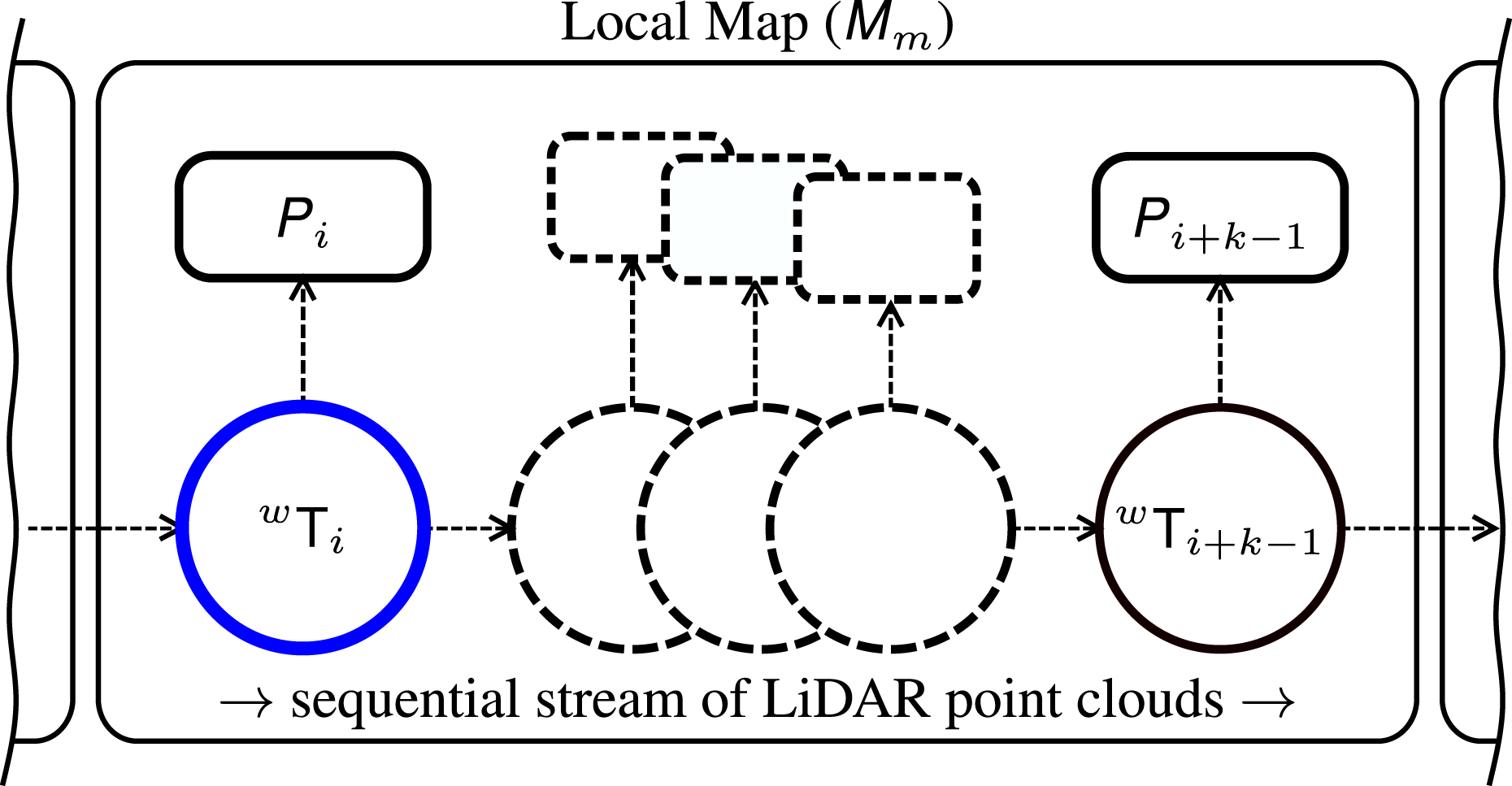
We transform each local map

Aggregating consecutive LiDAR scans into local maps provides richer structural information than individual scans, as illustrated in Figure 3. This larger spatial context is particularly beneficial in multi-session scenarios, where local environmental changes may otherwise hinder place recognition. Furthermore, local maps generated at the same location exhibit higher similarity across different LiDAR resolutions and scanning patterns, whereas inter-LiDAR place recognition with individual scans remains a challenging data association problem, even for humans, as illustrated in Figure 3. As a result, the use of local maps improves robustness for multi-session and cross-platform loop closure detection. A comparison of data from LiDARs with different scanning patterns and FoVs. The first row shows a single scan from an Ouster OS2-128 LiDAR with a 360° × 22.5° FoV and its corresponding local map. The second row shows a Livox Avia LiDAR with a 70° × 77° FoV and its corresponding local map. The similar structural features across local maps are highlighted with ellipses.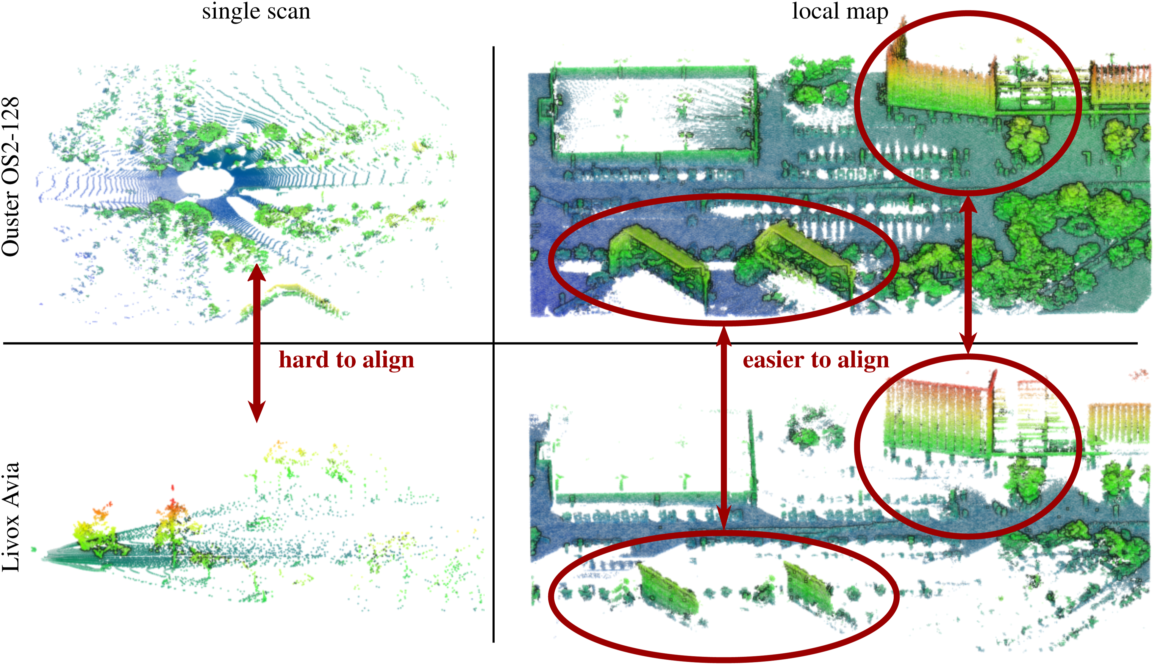
3.2. Ground plane detection and alignment
After generating the point cloud local map Effect of ground alignment on a local map generated from a handheld LiDAR sensor, recorded in a forest, with non-planar motion. The colors of the points represent their z-coordinates in the local reference frame. Left: Our ground alignment approach samples ground points 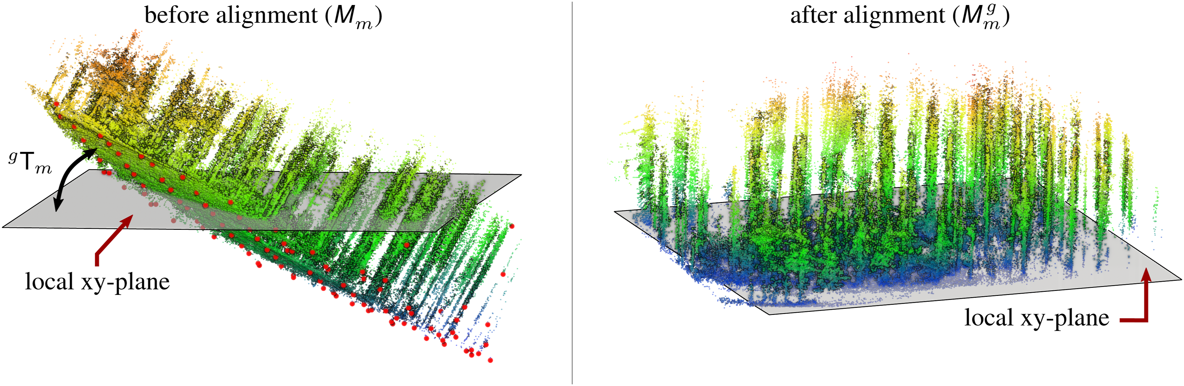
The first step identifies candidate ground points in the local map. Semantic segmentation networks can label ground in point clouds (Paigwar et al., 2020; Xu et al., 2021a), but they require offline GPU training and add significant computational costs. Real-time CPU-based methods such as Patchwork (Lim et al., 2021) and Patchwork++ (Lee et al., 2022) operate on individual scans, so they require per-scan segmentation and careful parameter tuning. In contrast, our BEV projection requires only one approximate estimate of the local ground plane to align the entire local map at once, not a precise segmentation for every scan.
We adopt a simple sampling strategy: in a 3D LiDAR local map, the lowest-elevation points usually correspond to the ground (Hu et al., 2014). This assumption generally holds for typical outdoor sensing platforms with known extrinsics, where the ground plane lies within the LiDAR’s field of view. It also remains valid when the local map’s xy-plane is not perfectly aligned with the ground plane, since a LiDAR cannot scan below the ground surface.
We divide the local map
We convert this PCA estimate into an initial transform


To make the ground alignment robust to outliers, we refine
We compute the Jacobian

The Jacobian indicates that the optimization only updates the z-axis translation and the roll (x-axis) and pitch (y-axis), which directly correct the ground alignment.
Finally, we apply the ground-aligning transform
3.3. Density-preserving bird’s-eye-view projection
After establishing the primary representation of the environment in Sections 3.1 and 3.2, the next step is to extract informative yet distinct local feature descriptors to perform place recognition for loop closures. Rather than computing features directly on the 3D point clouds of local maps, which is computationally expensive given the spatial extent of such point clouds, we use a 2D BEV projection of the local maps as an intermediate representation for loop closure detection.
We perform the BEV projection by simply dropping the z-coordinate of all the individual points in the ground-aligned local maps
However, the dimensionality reduction comes at the cost of losing the complete 3D information about the scene. Many traditional BEV projection approaches store the maximum elevation of the points in each cell (Kim et al., 2021; Kim and Kim, 2018; Li and Li, 2021; Luo et al., 2022). The maximum elevation, however, is sensitive to the distance between the scanner and the surface being scanned, as well as the LiDAR sensor’s FoV. In our pipeline, we instead store the point density in each discrete 2D cell after the projection, which is less sensitive to viewpoint changes (Luo et al., 2021).
Therefore, each cell in this grid

To mitigate the undesired influence of dynamic objects that accumulate during local map generation, we explicitly set all image pixels
3.4. Feature detection and pruning strategy
The BEV projection reduces the dimensionality of the local map, making feature detection for place recognition computationally efficient. The image-like BEV density representation enables us to apply well-established computer vision techniques to extract distinctive feature descriptors. Since these BEV density images preserve the geometrical, floorplan-like structure of the environment, we use ORB (Rublee et al., 2011) feature descriptors to capture relevant features. Unlike camera images, BEV images generated via orthographic projection have no scale ambiguity. We take advantage of this property by computing the ORB feature descriptors
Figure 5 shows an example of ORB features extracted from a BEV density image. We observe that most ORB features concentrate around high-density regions with strong gradients. These strong responses typically arise from static structures with large vertical footprints, such as building facades, trees, and light poles. In contrast, low-density regions, often corresponding to small bushes, vegetation, or dynamic objects that occasionally pass through the low-density filter, contribute few ORB features to the database. This leads to a robust behavior of our algorithm as it is not adversely affected by dynamic objects in the environment. A BEV density image of a local map, where darker pixels indicate higher point density. Red dots mark the ORB features extracted from the image.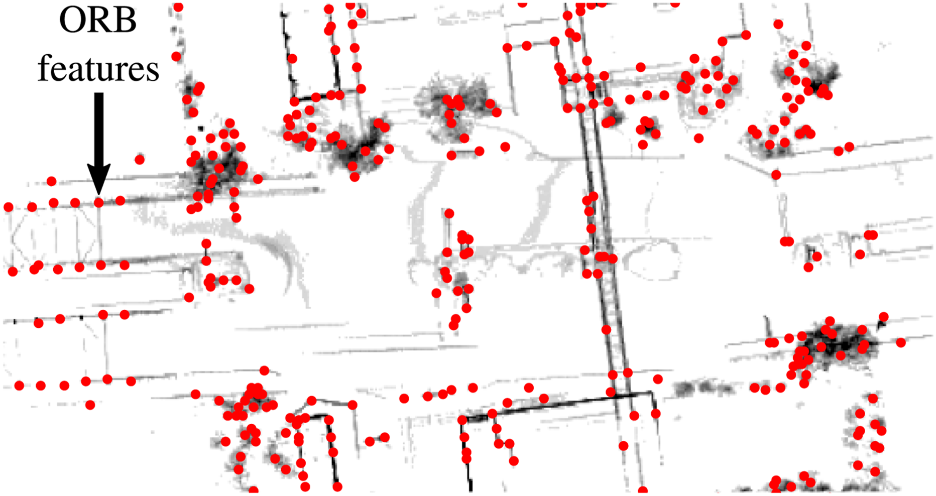
ORB feature descriptors remain salient within a local neighborhood of the density image, but not necessarily across the entire image. As a result, environments with repetitive structures can generate self-similar feature descriptors that can confuse the feature-matching stage and cause false positives.
To improve robustness against perceptual aliasing, we prune the ORB feature descriptors within each density image using a self-similarity check inspired by Bosse et al. (2004). Specifically, we compute the nearest-neighbor match for each ORB feature descriptor based on the Hamming distance and discard any feature whose closest match lies below a threshold of τ pr = 35 bits. This procedure eliminates self-similar feature descriptors within the same density image. This approach resembles Lowe’s ratio test (Lowe, 2004), but we apply it intra-image rather than inter-image, which avoids the cost of finding second-best matches across a larger feature descriptor database.
This pruning step filters out features from repetitive structures in the environment, such as repeating trusses on a bridge, as shown in Figure 6. This helps reduce false-positive feature matches across density images resulting from perceptual aliasing, thereby lowering the risk of incorrect loop closure detections. We present a detailed analysis of this pruning strategy and its impact on loop closure detection in Section 5.4. An example of self-similarity feature pruning applied to ORB feature descriptors computed on a BEV density image of a bridge with repetitive mechanical structures. Our algorithm prunes the features shown in red and retains those in green.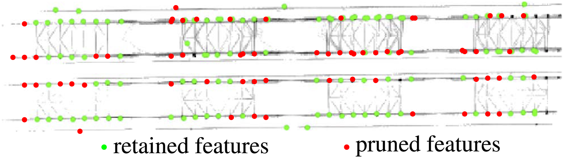
3.5. Feature database
Once we have the unique features within a BEV density image, we create a database to serve as a reference for place recognition. We leverage the binary domain of the ORB descriptors, using the Hamming distance embedding binary search tree (HBST) (Schlegel and Grisetti, 2018) to store the set of feature descriptors
The depth of the HBST is limited by the number of bits in the binary descriptor. As a result, a query descriptor will require at most 256 bitwise comparisons with the tree’s nodes before reaching a leaf node. Each leaf node can hold a maximum of 100 descriptors, ensuring efficient feature matching. These design choices constrain the computational time for feature matching without imposing practical limitations on the usability of our approach. Unlike a clustering-based bag of words or a neural representation-based database, we use the HBST as an incrementally updated database, requiring no offline pre-training.
After obtaining a set of descriptors ORB descriptor matches between features from a reference and a query BEV density image obtained from the HBST database. The inlier correspondences obtained from the RANSAC-based geometric verification are shown with green lines, and the outlier correspondences with red lines.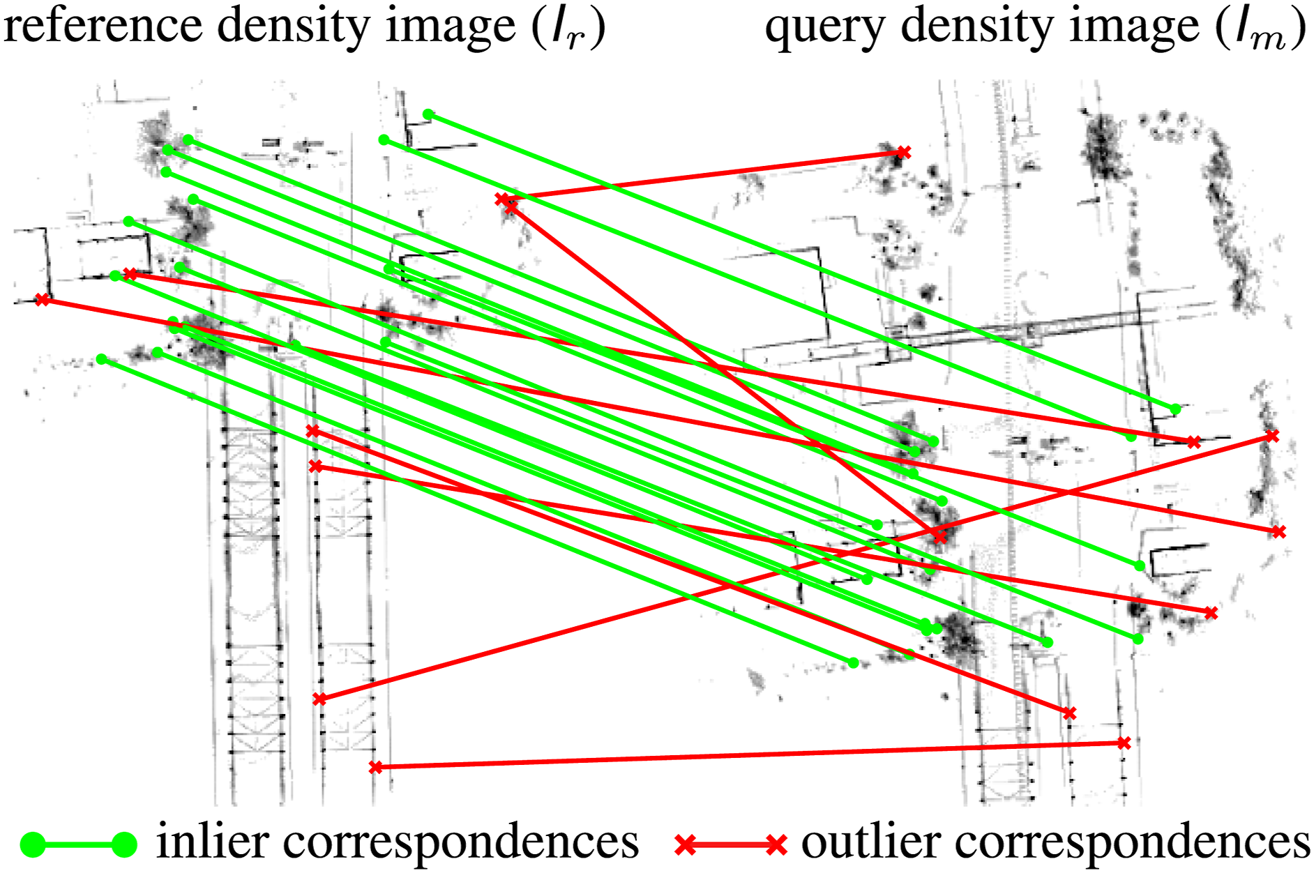
3.6. Loop detection and map alignment
The geometric validation step entails performing a 2D alignment of the matched ORB features. This involves computing a 2D rigid-body transformation that optimally aligns the matched features from the binary search tree using a distance metric. Unlike the general image-alignment problem, this process is constrained to an
We design a RANSAC-based approach that randomly selects two feature pairs from the set of matches between a query (
Finally, after the Nransac iterations, we compute a Kabsch-Umeyama 2D alignment over the entire set of inlier correspondences. It provides us with a rotation matrix
Although

This 3D alignment serves as an initial estimate for a fine-grained registration of local maps during typical pose-graph optimization in a SLAM pipeline. A qualitative example demonstrating the effectiveness of this initial alignment is illustrated in Figure 8. Notably, one of the local maps (in blue) in this visualization contains a large trace from a dynamic object (highlighted by the green ellipse), showing that our pipeline can also detect and align loop closures even in the presence of such strong dynamics. Two local maps (in red and blue) detected as loop closure and aligned using the initial estimate 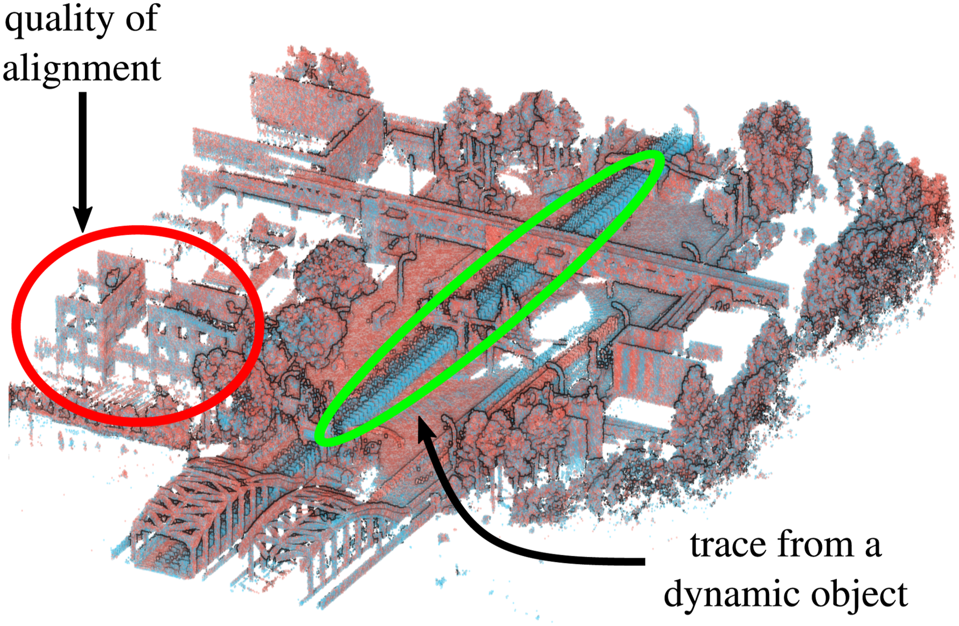
4. Experimental setup for evaluation
This section presents our experimental setup for evaluating our method and comparing it to existing loop closure detection approaches. We begin by introducing the datasets we use for evaluation and benchmarking. Next, we provide details about the implementation of the baseline methods we include in our comparison. Finally, we describe the quantitative metrics we use to assess the performance of our loop closure detection pipeline and the competing baselines.
4.1. Datasets
We conduct a comprehensive evaluation of our approach on datasets collected using a variety of LiDAR sensors with different resolutions and scanning patterns. These datasets include multiple sequences recorded in diverse urban environments across various mobile platforms.
4.1.1. Public datasets
We use the MulRan (Kim et al., 2020) and HeLiPR (Jung et al., 2024) public datasets, both recorded in urban environments using LiDAR sensors mounted on car rooftops. These datasets are well-suited for intra-session loop closure evaluation due to frequent in-sequence revisits with varying orientations and lane shifts. In addition, both datasets include at least three sequences per environment, making them ideal for evaluating inter-session loop closure detection.
The MulRan dataset was recorded using a 64-beam rotating LiDAR (Ouster OS1-64) operating at 10 Hz. Its horizontal FoV is limited to 290° due to occlusion from a radar sensor mounted behind it. We use sequences from three environments: KAIST, Riverside, and Sejong.
The HeLiPR dataset features multiple LiDAR sensors with different FoVs, scan patterns, and resolutions mounted on a single vehicle, enabling the evaluation of inter-LiDAR loop closure detection. From this dataset, we use three of the four available LiDARs: (i) a 128-beam spinning LiDAR (Ouster OS2-128) with 360° × 22.5° FoV, (ii) a hybrid solid-state LiDAR (Livox Avia) with 70° × 77° FoV and an unusual non-repetitive scanning pattern, and (iii) a solid-state LiDAR (Aeva Aeries II) with 120° × 19.2° FoV. We exclude the fourth sensor (Velodyne VLP-16) due to self-occlusion caused by surrounding sensors. The Bridge sequences in this dataset pose an additional challenge due to strong perceptual aliasing from repetitive structures in certain regions.
Moreover, both MulRan and HeLiPR datasets include sequences from the KAIST and Riverside environments, recorded approximately 4 years apart. This allows for a realistic evaluation of long-term inter-session loop closure detection, including cross-dataset comparisons between sequences captured with different LiDAR sensors. The KAIST and Riverside sequences also have some spatial overlap, providing an opportunity to evaluate multi-map alignment in a more challenging setting.
Additionally, we use two sequences from the NCLT dataset (Carlevaris-Bianco et al., 2016), recorded using a Velodyne HDL-32E LiDAR mounted on a Segway robot. The motion of the LiDAR in these sequences is non-planar due to the inverted pendulum-like dynamics of the Segway platform. We select two sequences recorded in the same environment but 1 year apart to assess the robustness of our loop closure detection approach under viewpoint and temporal variation.
4.1.2. Self-recorded datasets
In addition to the public datasets described above, we evaluate our approach on sequences recorded using our own instrumented vehicle and sensor platform. The IPB-Car sequence was recorded using an Ouster OS1-128 LiDAR mounted on the rooftop of an instrumented vehicle. We collected this data by driving through a hilly, semi-urban area with forest-lined roads and performing multiple revisits from varying viewpoints.
The IPB-Backpack sequence was captured using a sensor platform mounted on a backpack and carried through urban streets. This setup uses a Hesai Pandar-128 LiDAR mounted approximately 2 m above ground level. Unlike vehicle-mounted systems, the walking motion introduces non-planar sensor trajectories and dynamic changes in the viewpoint. This sequence presents a challenging test case for evaluating our ground alignment strategy under non-planar motion.
The two sequences share a small physical overlap in their environments, which we utilize to evaluate inter-session loop closure detection.
We generate near-ground-truth pose information using the offline LiDAR bundle adjustment method by Wiesmann et al. (2024), with manual inspection of the results to ensure alignment accuracy. This method incorporates RTK-GNSS data for geo-referencing; an information not provided to any loop closure system under evaluation. The process begins with initial pose estimates obtained from pose-graph fusion of LiDAR odometry (Vizzo et al., 2023), aided by either manually added loop closures (for the IPB-Backpack sequence) or RTK-GNSS data (for the IPB-Car sequence) to enforce global consistency. The final bundle adjustment refines these initial poses by aligning all scans with each other in an offline fashion.
4.2. Baseline methods used for comparison
We compare our approach against seven baseline methods, all of which provide publicly available implementations that we use for evaluation. To ensure a fair comparison, we modify their source code only to return multiple loop closure candidates per query scan rather than just the top-ranked one. Unless stated otherwise, we retain the default parameter settings in each baseline’s implementation.
4.2.1. Our approach
For our approach, we limit the maximum range of each LiDAR scan to 100 m. We set the travel displacement threshold τ c for generating local maps to 100 m as well. For KISS-ICP (Vizzo et al., 2023) odometry, we use their latest open-source version (v1.2.3). We use a voxel size of νmap = 0.5 m for the voxel grid used to generate the local maps, and the resolution of the BEV density images νb is set to 0.5 m. We use the default parameters for ORB feature descriptors, except that we turn off the scale invariance since the BEV images are orthographic projections. We obtain feature matches from HBST using a Hamming distance threshold of 50 bits and leave all other HBST parameters at their defaults. Finally, we classify two local maps as loop closures if the RANSAC-based alignment yields more than γ = 5 inliers.
For multi-session experiments, we save the HBST database from the reference session and use it as the database for the query session. We apply the same configuration to evaluate our previous approach, referred to as MapClosure (Gupta et al., 2024).
4.2.2. Scan context (SC)
Scan Context (Kim and Kim, 2018) is a widely used, state-of-the-art approach for LiDAR-based loop closure detection. However, it is specifically designed for LiDARs with a large horizontal FoV and a cylindrical scanning pattern. Therefore, we omit evaluation on the Livox Avia and Aeva Aeries II sensors from the HeLiPR dataset.
4.2.3. Stable triangle descriptors and binary triangle combined descriptors
STD by Yuan et al. (2023) introduces a triangle descriptor for point cloud local maps, which BTC (Yuan et al., 2024) extends with a binary descriptor for efficient storage and fast retrieval of loop closure candidates. Both methods accumulate 10 consecutive scans into a local map to compute descriptors. We use KISS-ICP to obtain the pose estimates for constructing these local maps. We adopt the default parameter settings from their implementations. For a fair comparison, we also evaluate STD and BTC on the same local maps used in our approach, generated with a 100 m travel displacement criterion. We refer to these variants as STD-100 and BTC-100.
4.2.4. Spatially organized and lightweight global descriptor (SOLiD)
SOLiD (Kim et al., 2024) is a recent loop closure detection method for 3D LiDAR sensors that is designed to operate across a wide variety of sensors, irrespective of their scan pattern, FoV, or resolution. The method employs a kd-tree-based search strategy to identify candidate loop closures. However, the authors do not provide an implementation of this search procedure in the publicly available codebase. Consequently, we approximate the candidate set by selecting all scans at least hundred frames prior to the current query scan. Following the procedure outlined in their manuscript, we compute the evaluation metrics using cosine distances between the descriptors of the query scan and each candidate.
4.2.5. LoGG3D-Net
LoGG3D-Net (Vidanapathirana et al., 2022) is a learning-based method that employs a 3D sparse convolutional network to extract consistent local features across different viewpoints. For our evaluation, we use the checkpoint trained on sequences from the MulRan dataset, as provided by the authors, and we adopt the default parameter settings from their implementation.
4.2.6. BEVPlace++
BEVPlace++ by Luo et al. (2025) is a learning-based method that computes a global descriptor for the BEV projection of the input scan using a rotation equivariant module. In our evaluation, we use the checkpoint trained on sequence 00 from the KITTI dataset (Geiger et al., 2013), as provided by the authors, and we adopt the default parameter settings from their implementation.
4.3. Reference loop closures between local maps
Since our method computes loop closures between local maps, we also define reference loop closures at the map level for evaluation. In contrast to prior works (Jiang and Shen, 2023; Kim et al., 2021, kim et al. 2024; Kim and Kim, 2018; Yuan et al., 2023), which typically rely on simple distance-based criteria, such heuristics are insufficient in our setting. The distance-based criterion breaks down in scenarios where other objects occlude the previously seen area, the sensor has a limited FoV, or the revisits are from a significantly different viewpoint. Additionally, there is inherent ambiguity in selecting the appropriate reference frame for measuring distances between local maps.
To overcome these limitations, we define reference loop closures based on the volumetric overlap of local maps, similar to Gupta et al. (2024) and Yuan et al. (2024). We generate reference local maps using the ground-truth pose information provided by the respective datasets. We ensure that each reference local map contains the same set of scans as the corresponding local maps produced by our method. We then identify reference loop closures by selecting all pairs of local maps that exhibit more than 25% voxel-level overlap. To avoid trivial short-range closures, we skip the three consecutive local maps preceding the query local map.
We adopt the same volumetric overlap strategy for cross-sequence evaluation, but reduce the overlap threshold to 10% to accommodate potential misalignments in the global pose information between sequences.
4.4. Scan-level to map-level conversion of loop closures for baselines
The baseline methods in our evaluation operate at different scales; some detect loop closures at the individual scan level (Scan Context and SOLiD), while others work on local maps with a fixed number of scans (STD and BTC). As a result, we cannot directly evaluate them using the reference loop closures defined between local maps generated based on a travel displacement criterion. Therefore, we convert their outputs into equivalent map-level loop closures.
For scan-level approaches, we treat a loop closure between scans
For methods such as STD and BTC, which use smaller local maps, we first extract all scan pairs between these local maps,
4.5. Evaluation metrics
4.5.1. Precision, recall, and F1 score
We use the reference closures computed in Section 4.3 to evaluate our approach and the baseline methods quantitatively. Specifically, we compute precision-recall curves by varying the threshold γ on the number of inlier feature descriptor matches from our pipeline’s RANSAC-based geometric validation stage. For the baseline methods, we generate their respective precision-recall curves by varying the key thresholding parameter described in their publications. In addition to the precision-recall curves, we report the average precision (AP) (area under the precision-recall curve), the maximum recall at 100% precision (R@1), and the maximum F1 score (F1 m ). We specifically choose to report R@1 as the maximum recall at 100% precision to emphasize the need to avoid false loop closures in a SLAM pipeline that could lead to catastrophic failures (Lowry et al., 2016).
4.5.2. Absolute pose error
We evaluate the effectiveness of our approach in correcting drift within a SLAM pipeline through an offline pose-graph optimization using the g2o optimizer (Kümmerle et al., 2011). We directly incorporate the detected loop closures between local maps as constraints in the pose-graph, using the initial transformation estimates from our pipeline.
We assess performance by computing the root mean square (RMS) absolute pose error (APE) in translation, with respect to ground-truth poses, both before and after the pose-graph optimization. To directly evaluate the accuracy of the detected loop closures and their alignments, we do not apply any robust kernel for outlier rejection during optimization.
We further evaluate the accuracy of the initial alignment estimate
5. Experimental evaluation
The primary focus of this work is an accurate and effective loop closure detection pipeline that works with various LiDAR sensors, invariant to their scanning pattern, FoV, and resolution. We present our experiments to show the capabilities of our method and support our key claims. Our approach (1) detects loop closures between local maps generated from various LiDAR sensors with different scanning patterns, FoVs, and resolutions; (2) performs multi-session loop closure detection and alignment with long-term revisits; (3) works with handheld platforms having non-planar motion in the LiDAR sensor frame; (4) is robust against perceptual aliasing in environments with repetitive structures; (5) provides a complete 3D rigid-body transform to align the detected loop closures; (6) detects loop closures between sequences having minimal overlap, recorded with different LiDAR sensor platforms, enabling cross-platform multi-map alignment.
5.1. Intra-session loop closure detection
In this experiment, we evaluate the performance of our approach on intra-session loop closure detection. We compare against several state-of-the-art baselines by converting their detected closures to local map-level closures, as described in Section 4.4. In addition, we include a comparison with our previous conference publication, MapClosure (Gupta et al., 2024), which forms the foundation of this work. We also evaluate the local map-based baselines STD and BTC using the same 100 m travel displacement-based local maps as in our approach, referred to as STD-100 and BTC-100. However, we do not evaluate the scan-based baselines using similar local maps since scan-based methods like Scan Context and SOLiD depend on a single scan center as the reference frame, which local maps inherently lack. Handling large lateral shifts would require sampling many artificial scan centers, changing the methods’ intended use.
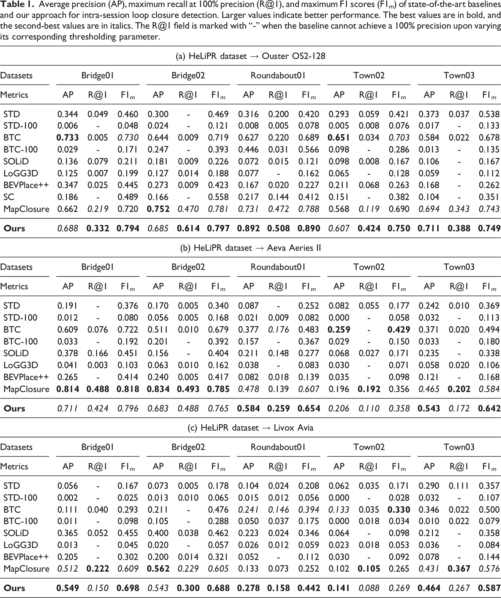
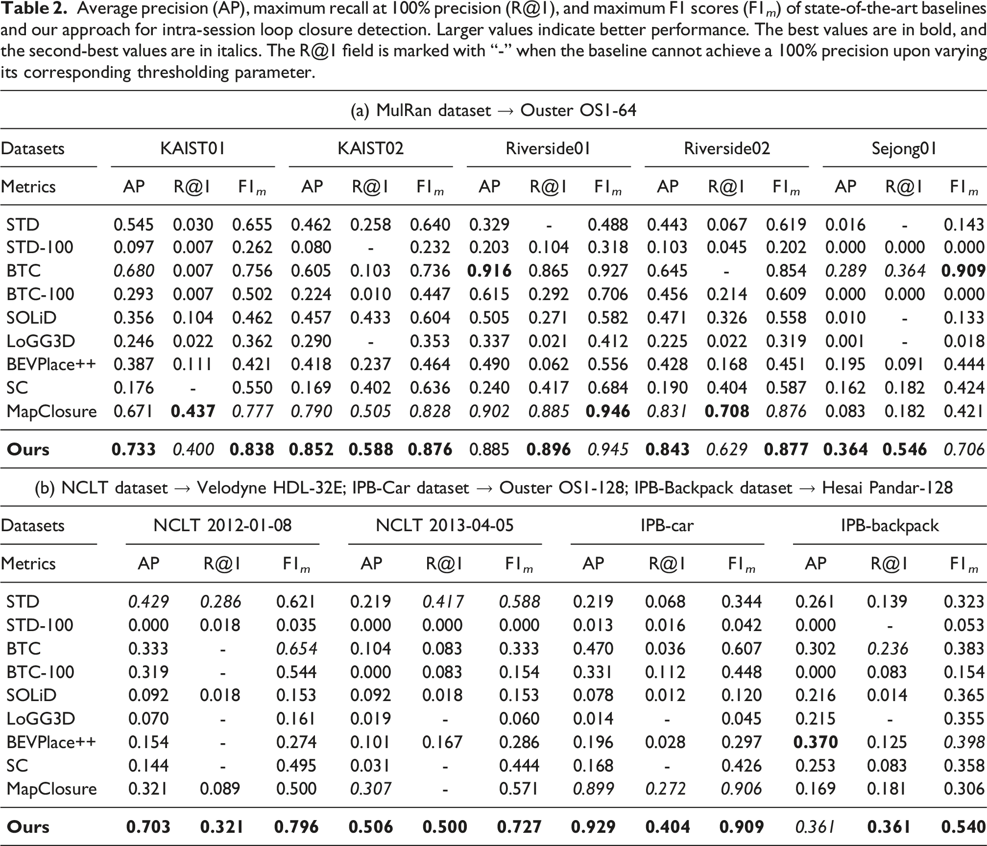
Average precision (AP), maximum recall at 100% precision (R@1), and maximum F1 scores (F1 m ) of state-of-the-art baselines and our approach for intra-session loop closure detection. Larger values indicate better performance. The best values are in bold, and the second-best values are in italics. The R@1 field is marked with “-” when the baseline cannot achieve a 100% precision upon varying its corresponding thresholding parameter.
Average precision (AP), maximum recall at 100% precision (R@1), and maximum F1 scores (F1 m ) of state-of-the-art baselines and our approach for intra-session loop closure detection. Larger values indicate better performance. The best values are in bold, and the second-best values are in italics. The R@1 field is marked with “-” when the baseline cannot achieve a 100% precision upon varying its corresponding thresholding parameter.
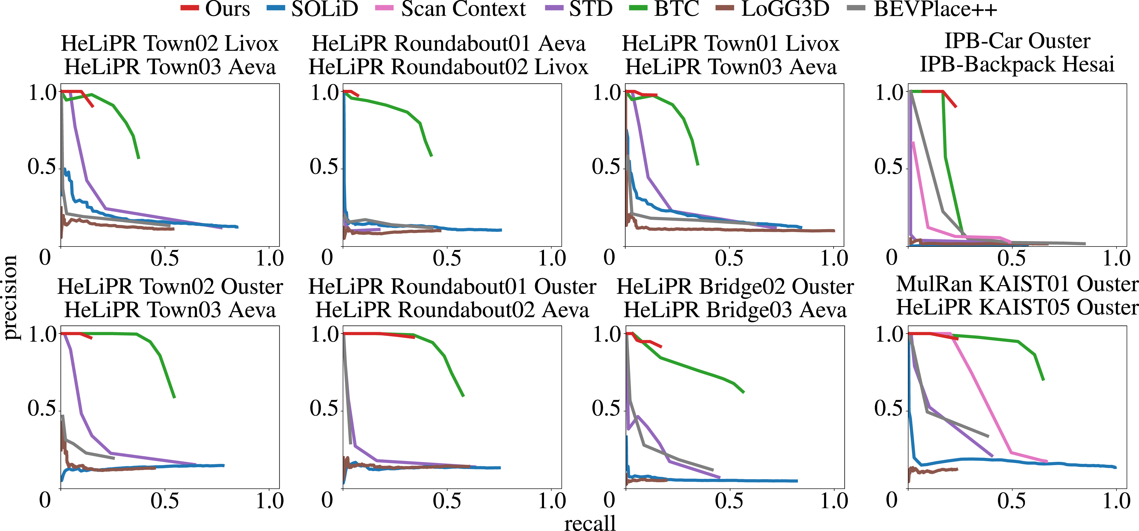
Our method provides a robust solution for loop closure detection within a SLAM pipeline, where false positives must be minimized (Bailey and Durrant-Whyte, 2006; Blanco et al., 2013; Lowry et al., 2016). The precision-recall curves in Figure 9 show that our approach (red) consistently outperforms baselines across datasets with varied sensor setups. It maintains high precision over a broad range of recall values, eliminating the need for careful tuning of the inlier threshold in RANSAC or additional outlier rejection schemes in the pose-graph optimization. The precision-recall curves of state-of-the-art baselines and our approach for intra-session loop closure detection.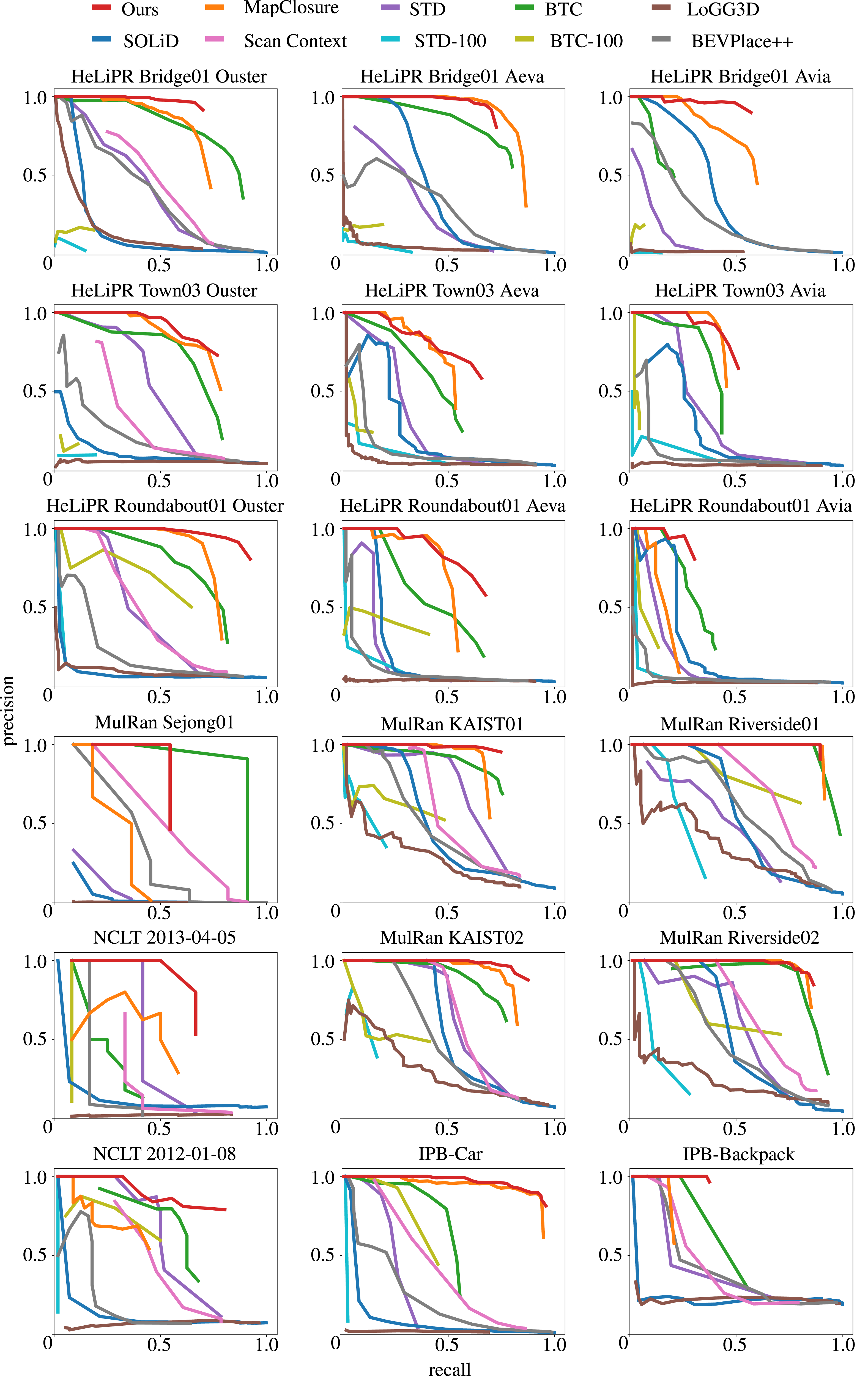
The evaluations on the HeLiPR dataset demonstrate the versatility of our method across different LiDAR sensors in varied urban environments. Our method consistently ranks among the top two methods across all metrics. In several sequences, our current approach ranks second only to MapClosure. However, the precision-recall curves in Figure 9 reveal a key advantage: our method maintains a higher precision than MapClosure, ensuring that detected loop closures remain accurate.
The HeLiPR Bridge sequences, which exhibit strong perceptual aliasing, highlight the effectiveness of our pruning strategy. While overall metrics in Table 1 may appear comparable between our method and MapClosure, our precision-recall curves in the first row of Figure 9 terminate earlier at a higher precision value than MapClosure, which also holds in comparison to other baselines. This behavior reflects our deliberate choice to prioritize precision over recall in perceptually ambiguous scenes. By doing so, we improve robustness, reduce sensitivity to the inliers threshold (γ), and lower the risk of false loop closures. The Town sequences present additional challenges with narrow alleyways, wide boulevards, and numerous dynamic objects such as pedestrians and cars. Even under these conditions, our approach ranks among the top two methods, showing its resilience in complex urban environments.
Additionally, the results on HeLiPR Bridge sequences provide insight into how the baselines perform under different levels of dynamic activity in the scene. The Bridge01 sequence, recorded at night, contains relatively few dynamic objects, whereas Bridge02, recorded during the day, includes substantially more dynamic participants. Since both sequences capture the same driving environment, we can directly compare their results to assess how dynamic objects affect loop closure detection. Our method performs consistently in terms of average precision and F1 score, highlighting its robustness to such dynamic elements. As expected, scan-based methods also show little to no variation in the metrics across these sequences, since individual scans are not significantly affected by dynamic objects due to the short temporal window of a single LiDAR scan.
The ground alignment strategy introduced in Section 3.2 further strengthens performance on datasets with non-planar LiDAR motion, such as the NCLT dataset and our self-recorded IPB-Backpack sequence. As shown in Table 2, our method outperforms Scan Context, BEVPlace++, and MapClosure, which assume planar motion for the BEV projection. We achieve the best values across all three metrics, except for average precision on the IPB-Backpack dataset, where the performance gap to BEVPlace++ remains marginal. Consistent BEV projection onto the local ground plane during revisits, even under varying pitch and roll, drives this performance. On the IPB-Car dataset, recorded in hilly terrain with vegetation and elevation changes, our method achieves almost 100% average precision, with a near-perfect precision-recall curve, confirming its robustness to complex ground plane variations.
The results also confirm the importance of local maps for extracting meaningful structural information for place recognition and loop closure detection. Among the baselines, only STD, BTC, and MapClosure perform competitively, and all rely on local maps. Nonetheless, our evaluation of STD and BTC with the same local maps as our pipeline, referred to as STD-100 and BTC-100, shows that our method’s advantage does not stem solely from larger local map sizes, but from the full algorithmic design.
In contrast, scan-based global descriptor approaches such as Scan Context and SOLiD fail to achieve consistent performance. Scan Context, designed for rotating LiDAR sensors, performs poorly in the HeLiPR Ouster OS2-128 and MulRan sequences due to its strong dependence on viewpoint. SOLiD, designed to handle LiDARs with different FoVs, performs better on the HeLiPR Aeva Aeries II and Livox Avia sequences but still falls short of local map-based methods. These trends highlight the inherent difficulty in constructing global descriptors for single LiDAR scans.
The weak performance of LoGG3D further illustrates this limitation. Without spatio-temporal aggregation or dimensionality reduction, LoGG3D remains highly sensitive to the point density within each scan. Trained exclusively on sequences from the MulRan dataset with Ouster OS1-64, it performs well only on that dataset and generalizes poorly elsewhere. It fails to reach 100% precision even at low recall values in most sequences, underscoring the need to retrain such methods for each sensor setup.
BEVPlace++, also a learning-based method, performs more robustly than LoGG3D does due to its density-preserving BEV projection. However, it struggles on NCLT and IPB-Backpack sequences because of its assumption of planar motion for BEV projection.
Overall, these experiments confirm our core claim: our method delivers state-of-the-art performance in intra-session loop closure detection across datasets and LiDAR platforms. By leveraging local maps as the core representation, our pipeline balances precision and recall, remains robust under perceptual aliasing, adapts to non-planar motion, and generalizes across different sensor characteristics, all without requiring changes to the pipeline parameters.
5.2. Inter-session and inter-LiDAR loop closure detection
In this experiment, we evaluate the performance of our approach for inter-session and inter-LiDAR loop closure detection and compare it against state-of-the-art baselines introduced in Section 4.2. We select sequences spanning revisit intervals from a few weeks to several years to test the robustness under diverse temporal conditions.
Our pipeline architecture remains fundamentally the same in this scenario, with only minor modifications. We store the ground alignment transformations for each local map together with the HBST database from the reference sessions. For a given query session, we match the ORB features against the reference database without adding any features from the query session to the database. Then, using the ground alignment transforms of the corresponding local map from the reference session and the query local map, we compute a complete
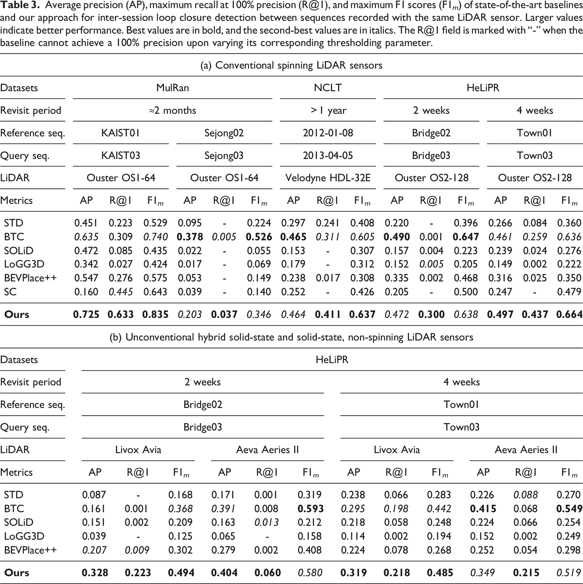
We first evaluate inter-session loop closures using the same LiDAR sensor. The precision-recall curves in Figure 10 and the metrics reported in Table 3 reveal trends consistent with the intra-session results. Our method consistently achieves the highest recall at 100% precision across different LiDARs and revisit periods, confirming its reliability in challenging conditions. The precision-recall curves highlight this robustness, as they terminate earlier but maintain high precision. Our method also ranks among the top two in average precision and maximum F1 scores, with BTC being the only baseline matching our overall performance. Other baselines often fail to reach 100% precision or achieve it only at very low recall, except in the MulRan KAIST01–KAIST03 sequences. The precision-recall curves of state-of-the-art baselines and our approach for inter-session loop closure detection. Average precision (AP), maximum recall at 100% precision (R@1), and maximum F1 scores (F1
m
) of state-of-the-art baselines and our approach for inter-session loop closure detection between sequences recorded with the same LiDAR sensor. Larger values indicate better performance. Best values are in bold, and the second-best values are in italics. The R@1 field is marked with “-” when the baseline cannot achieve a 100% precision upon varying its corresponding thresholding parameter.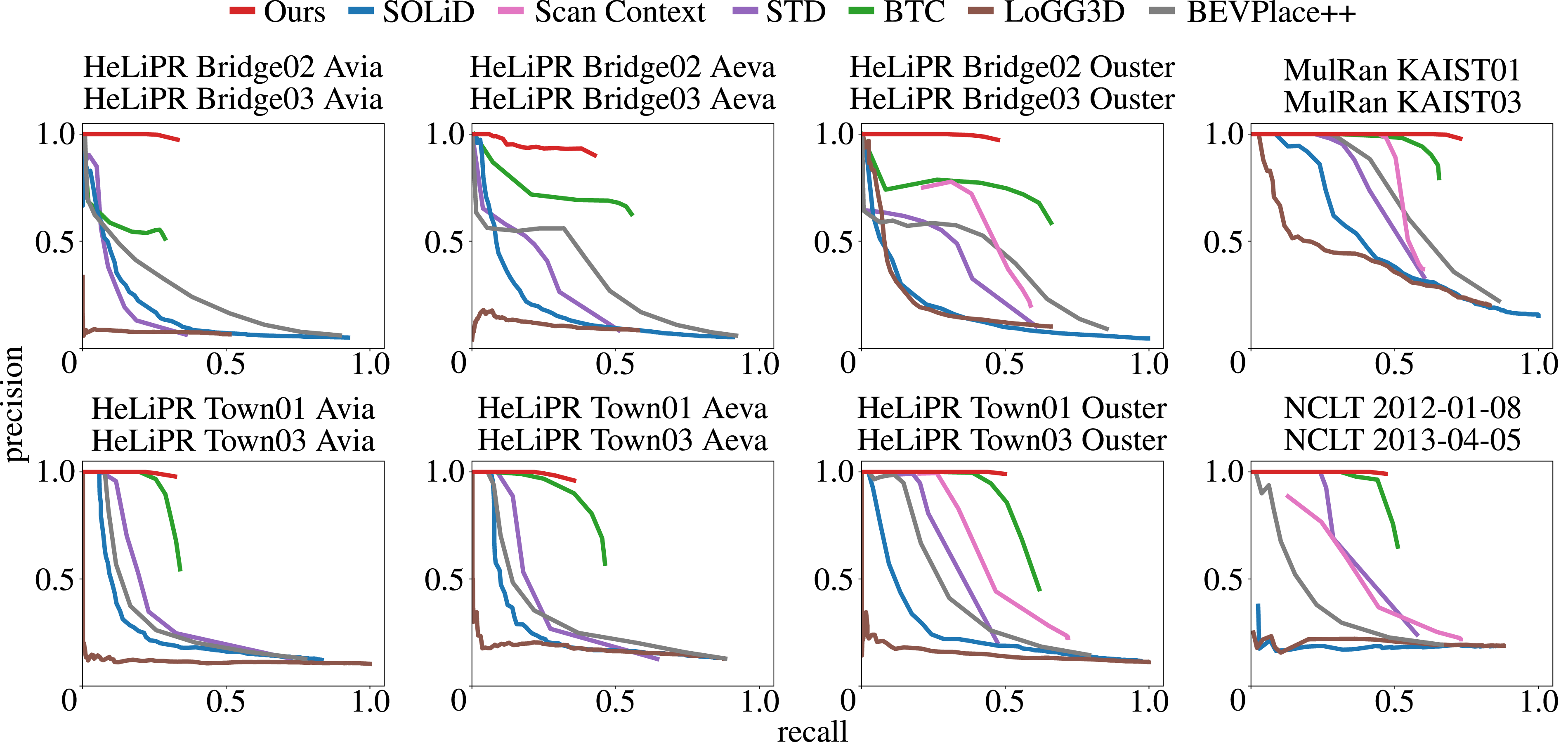
The Sejong02–Sejong03 sequences from the MulRan dataset were recorded as opposite-direction traversals on a long highway, which produces sparse structural geometry throughout the sequences. The restricted FoV of the dataset’s LiDAR further increases the difficulty of inter-session loop closure detection. As shown in Table 3a, all baselines perform substantially worse on this pair of sequences, especially when we compare their results to those on the KAIST01–KAIST03 sequences from the same dataset, recorded with the same setup but in a dense urban environment.
The Bridge sequences from the HeLiPR dataset underscore the benefit of our self-similarity pruning strategy. Strong perceptual aliasing causes most baselines to either miss 100% precision entirely or reach it only at negligible recall. Even BTC, which performs comparably to our method in most other scenarios, fails to maintain its high precision on the Bridge sequences because it lacks an explicit mechanism to handle perceptual aliasing. In contrast, our approach detects accurate loop closures at comparatively higher recall, as reflected in the clear separation of our precision-recall curves from the baselines.
Additionally, we achieve better performance across different LiDAR sensors on the same sequences without changing any parameters in our pipeline. As shown in Table 3b, the Aeva Aeries II LiDAR experiences a sharp drop in maximum recall at 100% precision on the Bridge02–Bridge03 sequences. This drop arises from the overlap threshold used to define ground-truth loop closures: a few valid closures fall below the threshold and are therefore marked as false positives in ground-truth local maps, which lowers the maximum recall at 100% precision. Nevertheless, the average precision and the corresponding precision-recall curve in Figure 10 demonstrate that our method still performs strongly, maintaining near-100% precision across a substantially larger recall range.
On the NCLT dataset, which includes a revisit after about 1 year with a low-resolution Velodyne HDL-32E LiDAR, our approach again achieves the best recall at 100% precision and maximum F1 score. Only STD and BTC are the baselines that perform comparably in this scenario. This emphasizes the importance of having explicit knowledge about the ground plane under non-planar LiDAR motion.
These results also highlight the challenges that scan-based global descriptor methods such as Scan Context, SOLiD, and LoGG3D face in long-term revisit scenarios. In such scenarios, significant lateral shifts, viewpoint changes during revisits, and scene changes can all alter the global descriptor substantially. In contrast, local map-based local descriptor methods like ours, STD, and BTC avoid these issues by aggregating multiple scans to reduce viewpoint dependence and by focusing on local regions of the scene that remain similar across revisits, rather than compressing the local context into a single global descriptor.
The results on the HeLiPR sequences further highlight the impact of the LiDAR type on long-term place recognition. Even among the stronger baselines, we observe a noticeable drop in performance when switching from a 360°-horizontal-FoV Ouster OS2-128 LiDAR to the limited-horizontal-FoV LiDAR sensors such as Aeva Aeries II and Livox Avia, even when evaluating the same pair of sequences.
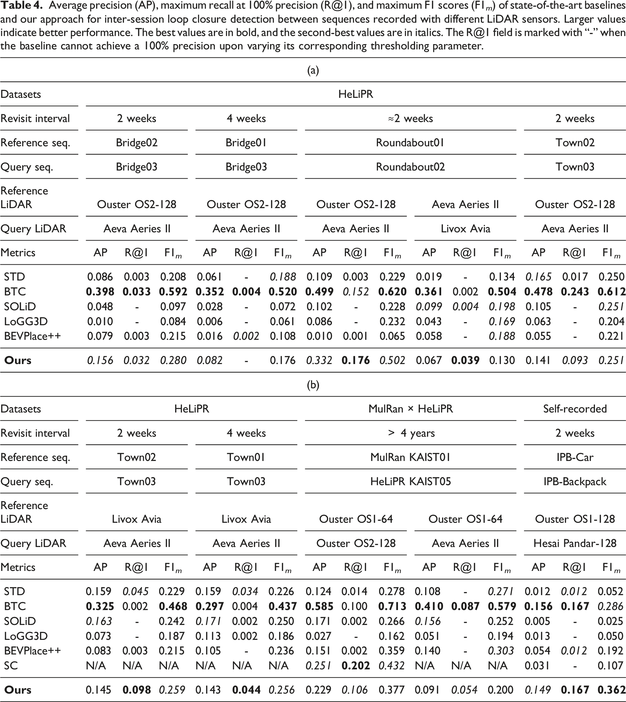
Average precision (AP), maximum recall at 100% precision (R@1), and maximum F1 scores (F1 m ) of state-of-the-art baselines and our approach for inter-session loop closure detection between sequences recorded with different LiDAR sensors. Larger values indicate better performance. The best values are in bold, and the second-best values are in italics. The R@1 field is marked with “-” when the baseline cannot achieve a 100% precision upon varying its corresponding thresholding parameter.
The precision-recall curves of state-of-the-art baselines and our approach for inter-LiDAR loop closure detection.
The performance of scan-based methods like Scan Context, SOLiD, LoGG3D, and BEVPlace++ is adversely affected by the difference in the scanning patterns, FoVs, and resolutions across LiDAR sensors. The local map-based methods achieve better results in such cross-LiDAR scenarios.
On the Roundabout01–Roundabout02, Town01–Town03, and Town02–Town03 sequences, our pipeline achieves the best recall at 100% precision among all baselines, demonstrating robustness to opposite traversals and constrained sensor views. However, on Bridge01–Bridge03 and Bridge02–Bridge03 sequences, the feature-pruning strategy limits recall to very low values, leaving room for improvement.
Cross-dataset evaluations between MulRan and HeLiPR push this further, with revisit intervals of over 4 years and different LiDAR sensors. These scenarios introduce structural changes in addition to sensor differences, making them highly challenging. Even so, our method achieves the second-best recall at 100% precision, while all baselines, including ours, achieve lower recall overall.
Finally, in self-recorded datasets collected 2 weeks apart with platforms having different motion profiles and LiDARs, our method performs comparably to BTC across all metrics, confirming its ability to generalize across diverse sensor setups.
Overall, these evaluations demonstrate that our approach effectively detects loop closures across multiple sessions for different LiDAR sensors and revisit intervals, thereby supporting our second key claim. At the same time, they highlight opportunities for further research on the highly challenging problem of inter-LiDAR loop closure detection.
5.3. Analysis and evaluation of the ground alignment module
In this section, we present both qualitative and quantitative evaluations of the ground alignment stage, which enhances the detection and alignment of loop closures. As we describe in Section 3.2, we need this stage in scenarios where the LiDAR experiences non-planar motion, allowing us to maintain a consistent reference plane for the BEV projection across revisits.
When we turn off the ground alignment module, our approach projects local maps onto the xy-plane, assuming planar motion. Consequently, using the RANSAC-based validation, it can align the local maps only along the xy-plane. We illustrate such a 2D alignment in the top-left image of Figure 12, where two local maps appear well-aligned from a top-down view. However, this alignment can be misleading. In the top-right image of Figure 12, a different perspective reveals an apparent misalignment in height and tilt between the two local maps, caused by non-planar LiDAR motion. Visual comparison of loop-closed local map alignments with and without ground alignment. The top-down view (xy) shows both local maps to be aligned in either case, as RANSAC operates in 2D. However, the side view (xz) reveals significant misalignment without ground alignment due to uncorrected pitch and roll differences, as highlighted by the black ellipse. Applying ground alignment provides consistent 3D alignment by projecting the local maps onto a common physical ground plane.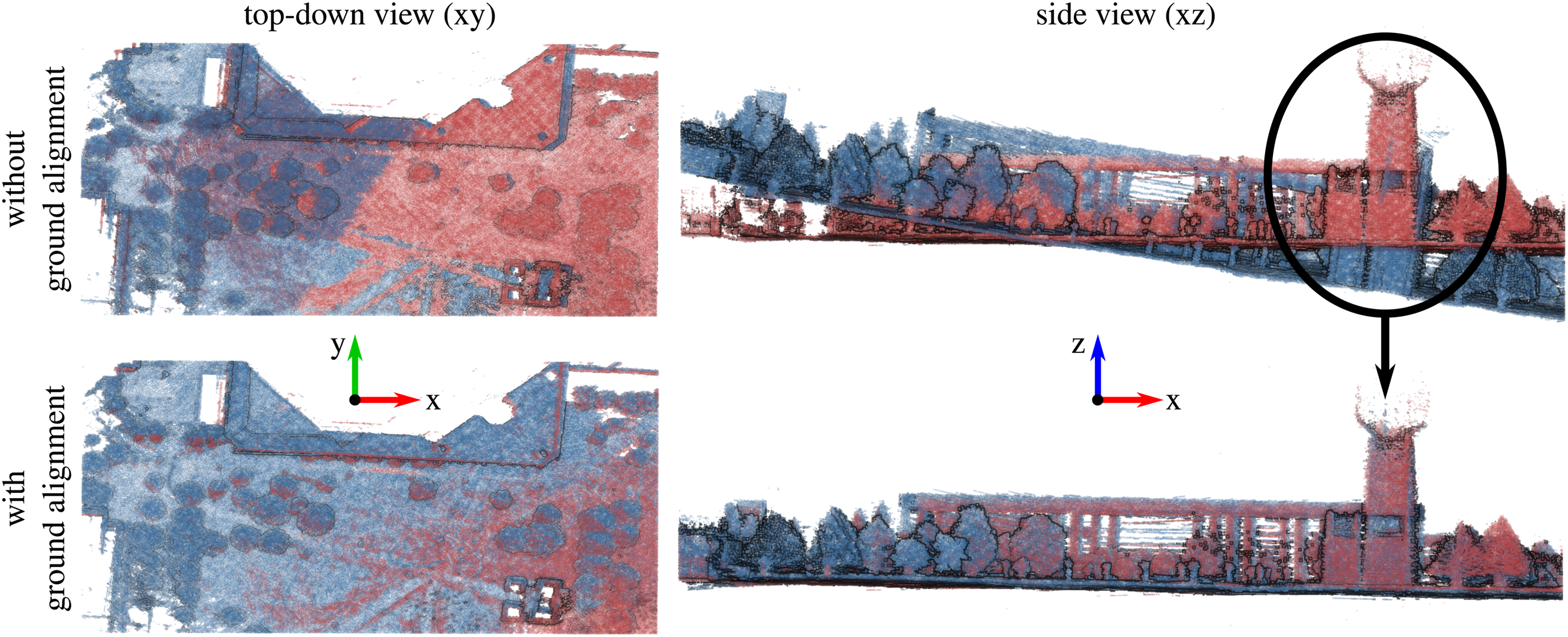
By applying explicit ground alignment, we ensure that the local maps involved in a loop closure align correctly in 3D. This improvement enables our method to perform complete 3D global alignment rather than relying solely on a 2D assumption. The second row of Figure 12 shows a more accurate initial alignment between the local map pairs, even before any point cloud registration takes place.
Evaluation of the ground alignment strategy for loop closure detection and local map alignment. We report the number of correctly identified loop closures and the root mean square (RMS) error in the overlap between aligned local maps using our pose estimate
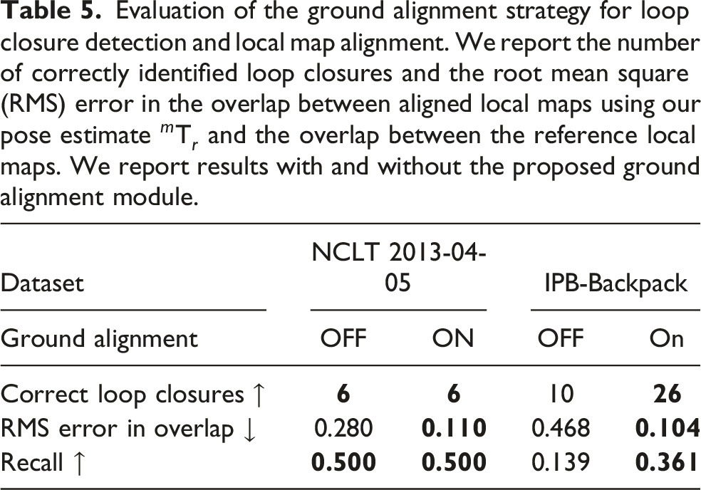
As seen in Table 5, the ground alignment stage significantly reduces the overlap error between local maps. This improvement occurs without applying any local point cloud registration. This advantage becomes evident in datasets with strong non-planar motion, such as the IPB-Backpack setup, where roll and pitch angles vary approximately between −30° and 30°. In such cases, the proposed ground alignment module enables our system to detect substantially more loop closures. This is because the BEV density images remain consistent across revisits when we project them onto the actual ground plane in the environment rather than onto the xy-plane of the local map frame.
We next evaluate the ability of our ground alignment module to correct misalignments between the ground plane and the map’s local xy-plane. To test this, we manually apply rotations in the range (10°–80°) about 10 random axes lying in the xy-plane of each reference local map. Our method then estimates the transform
In Figure 13, we report the mean and standard deviation of the absolute error in the predicted rotation magnitude, averaged across all 10 axes for each local map, as a function of the applied misalignment. The ground alignment module reliably corrects misalignments up to 60°, with a mean error below 1° and a standard deviation below 8°. Even at initial misalignments of around 80°, the mean absolute error typically remains below 10°, except in the Livox Avia sequence, where observed failures stem from the Livox Avia sensor’s unusual reflective artifacts. These artifacts produce misleading, consistently oriented below-ground points that disrupt low-lying points sampling and PCA filtering under artificially large rotations. We would like to highlight that this is a sensor-specific quirk and not a flaw in the alignment method. However, since real-world misalignments rarely approach such extreme values, this level of performance is sufficient for practical use. Quantitative evaluation of the ground alignment accuracy. The azimuthal axis indicates the absolute initial misalignment magnitude between the ground plane and xy-plane of the local maps. The radial axis (log scale) shows the absolute error of the predicted ground alignment magnitude, reported as mean values (dots) and standard deviation (bars), across different sequences and LiDARs from the MulRan and HeLiPR datasets.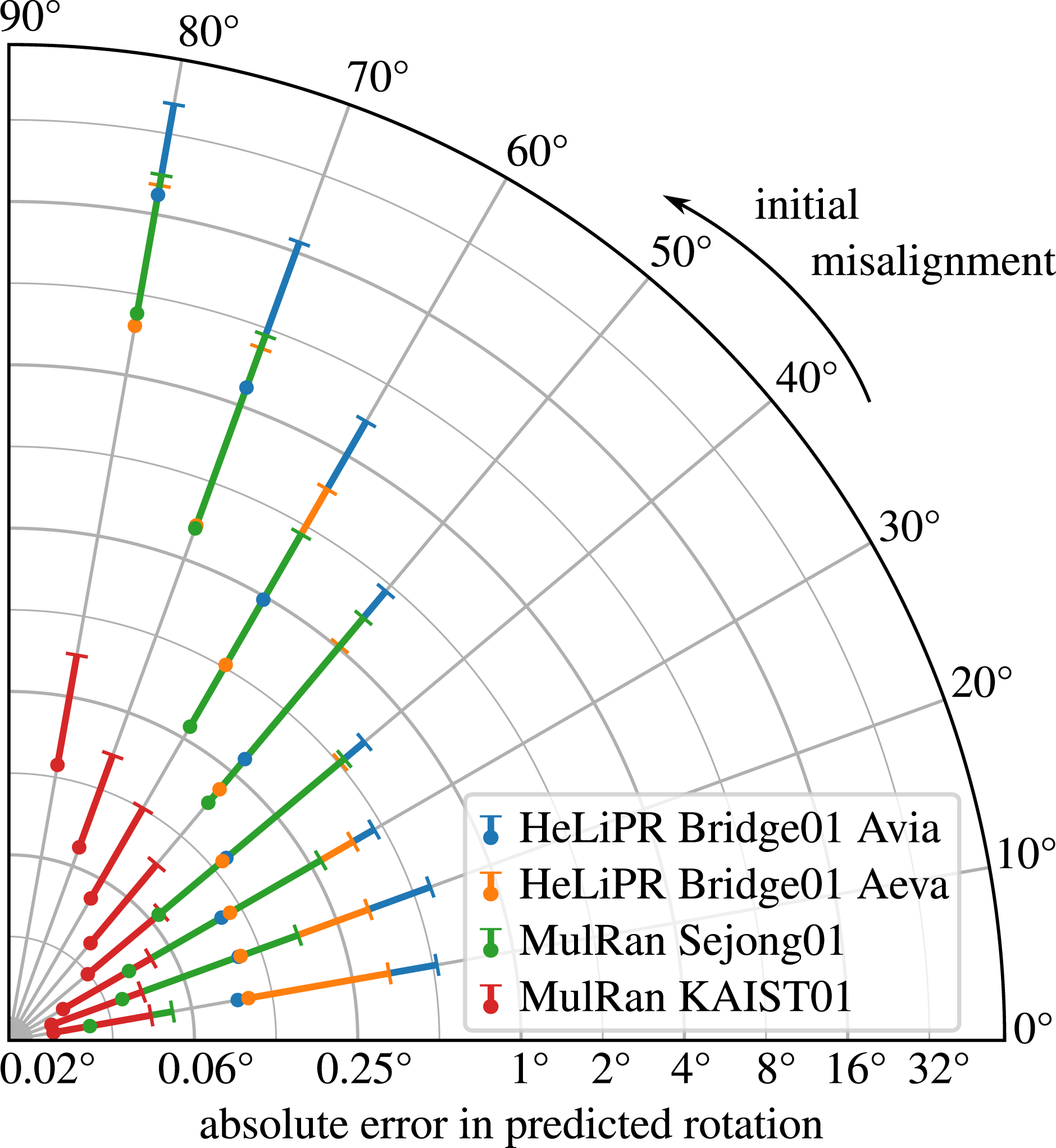
These results support our third claim that the proposed ground alignment module enables robust handling of handheld or non-planar LiDAR motion and also provides a strong initial pose estimate for the 3D alignment of loop-closed local maps.
5.4. Analysis and evaluation of the self-similarity pruning strategy
In this section, we evaluate the effectiveness of the self-similarity pruning strategy in detecting loop closures within environments characterized by highly repetitive structures. Specifically, we focus on the Bridge sequences from the HeLiPR dataset, which feature long bridges composed of repeating mechanical elements. These conditions present significant challenges due to perceptual aliasing, which can lead to false loop closures.
Figure 14 shows a zoomed-in precision-recall curve for different self-similarity pruning thresholds based on the Hamming distance between ORB descriptors. The mark X on the curve represents the performance at an inlier threshold of 5, the default setting in our pipeline. Lower threshold values prune only strictly similar features, leading to higher recall values but a drop in precision, similar to the performance without pruning. Conversely, higher thresholds prune more features, leading to a drop in recall but maintaining high precision. The threshold value of 35 provides a desirable trade-off, maintaining a recall of around 0.6 with minimal loss in precision. Precision-recall curves for various choices of pruning thresholds in terms of the Hamming distance between ORB descriptors. We visualize a zoomed-in precision-recall curve for better differentiation between different curves.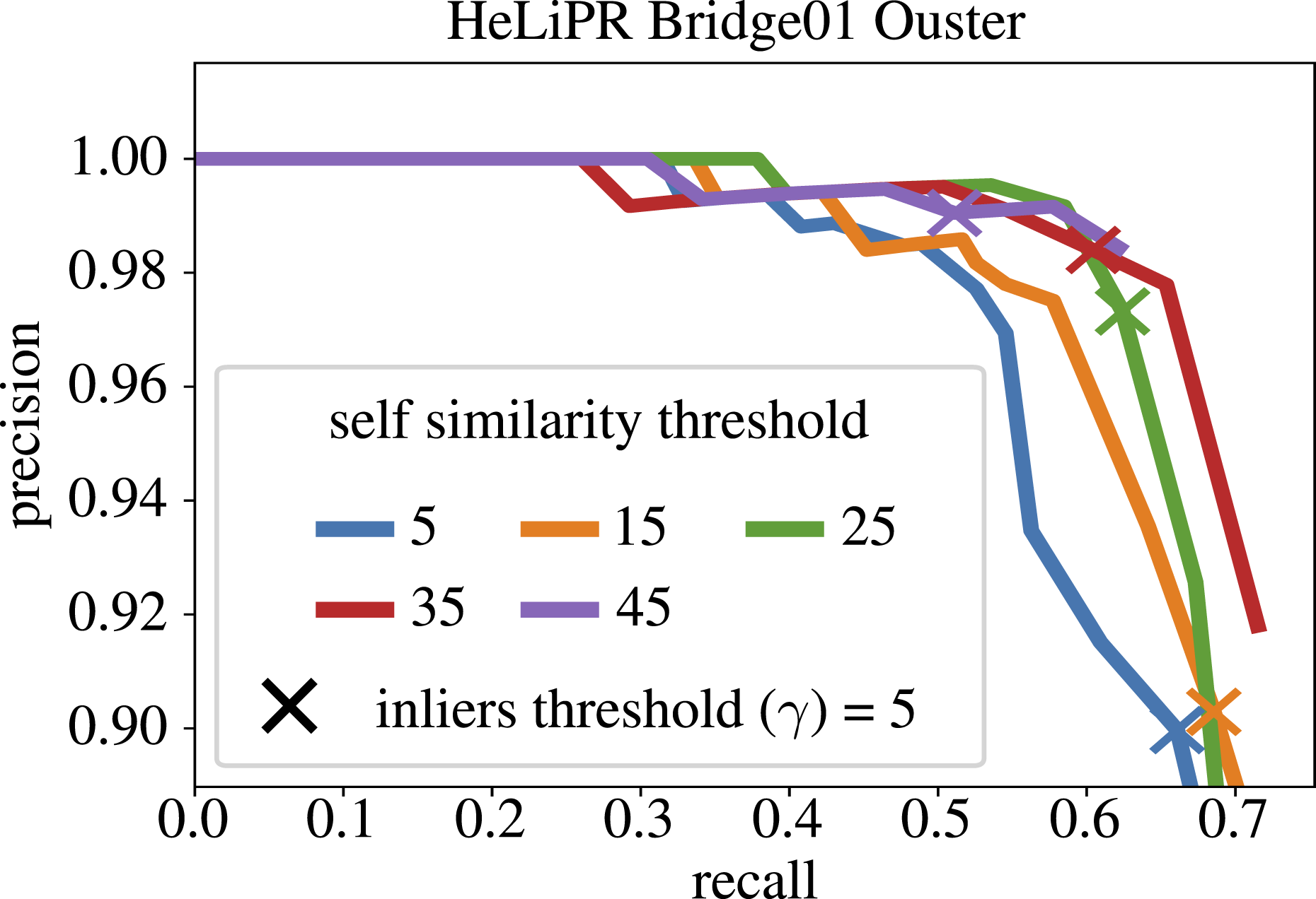
Without the pruning strategy, our method detects false loop closures in these Bridge sequences. We show one example at the bottom-left of Figure 15, where a false match occurs with a near-perfect alignment between local maps. This alignment is supported by a sufficient number of inlier correspondences after a 2D RANSAC alignment of their BEV features (right-hand side of Figure 15), primarily caused by repetitive structures on the bridge. We successfully eliminate these matches between similar structures by applying the feature pruning strategy described in Section 3.4, thereby preventing the false loop closure. Precision-recall curves evaluating the impact of the pruning strategy for loop closure detection on the Bridge sequences from the HeLiPR dataset. These sequences are recorded in an environment with strong perceptual aliasing. ambiguous, repetitive features that lead to perceptual aliasing.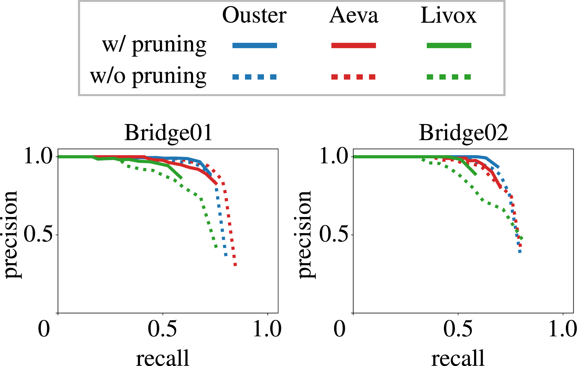
We further compare the performance of our pipeline with and without feature pruning in Figure 16. The precision-recall curves for both configurations, across the two Bridge sequences and three different LiDAR sensors, show that our approach with pruning maintains high precision throughout rather than compromising on precision to achieve a better recall. In contrast, our approach without pruning achieves slightly higher recall but significantly drops precision. Visualization of perceptual aliasing in the HeLiPR Bridge sequence and the impact of feature pruning on loop closure detection. Left: The repetitive semi-circular arches of the bridge (top) lead to structurally similar local maps (below) as highlighted by the yellow ellipses, causing a false loop closure. Right: Feature correspondence plots before and after pruning. Without pruning, RANSAC mistakenly accepts many inlier correspondences (green lines), resulting in a false positive. After pruning, only outlier matches (red lines) remain, correctly preventing erroneous loop closure. Feature pruning effectively removes ambiguous, repetitive features that lead to perceptual aliasing.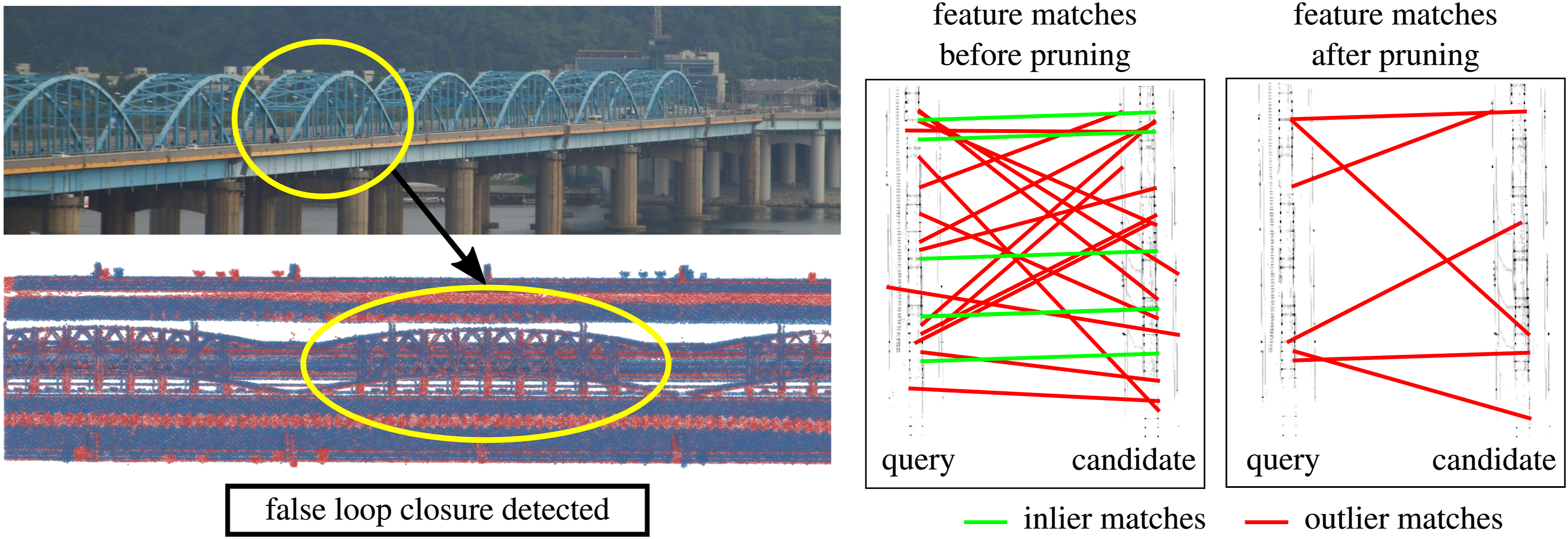
The effect of feature pruning on loop closure accuracy, measured by RMS APE w.r.t. translation after pose-graph optimization. We report the results for three LiDAR sensors across two sequences from the HeLiPR dataset.
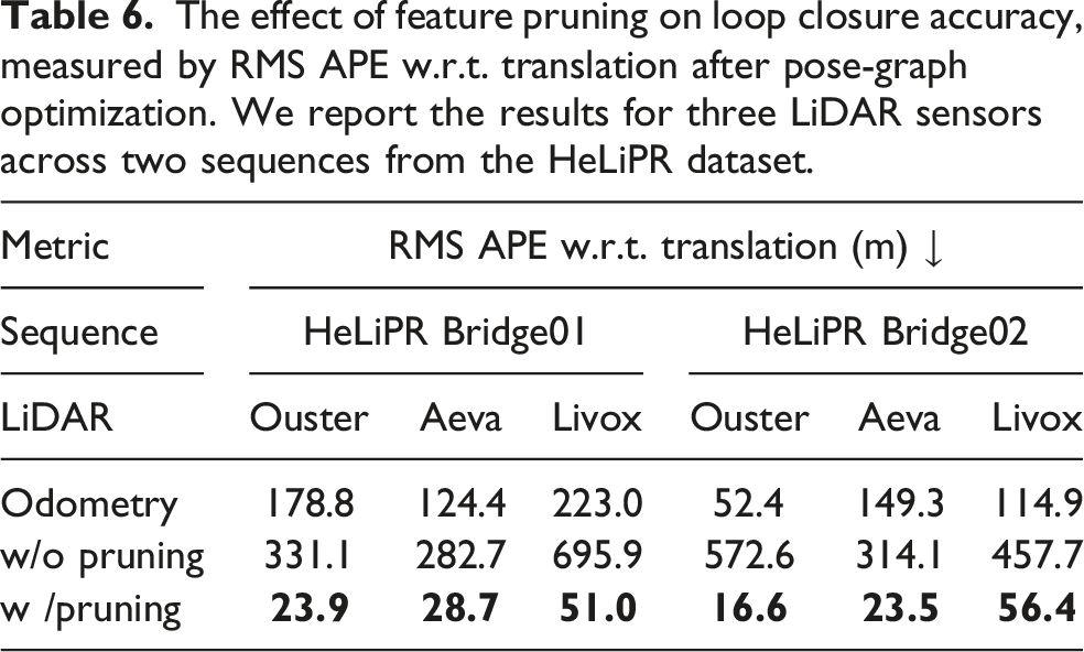
Overall, this study supports our fourth claim that the self-similarity feature pruning strategy introduced in Section 3.4 is essential for maintaining robustness in loop closure detection under high structural repetition. By prioritizing precision, our method avoids catastrophic failures in pose estimation, ultimately leading to more reliable mapping and localization.
5.5. Evaluation of the 3D alignment estimates
In this section, we evaluate the accuracy of the initial alignment
Evaluation of the loop closure alignment accuracy. We report accuracy in terms of RMS APE in translation (m) and rotation (°) compared to the proxy ground-truth alignment obtained via Open3D point-to-point ICP. Best results are in bold.
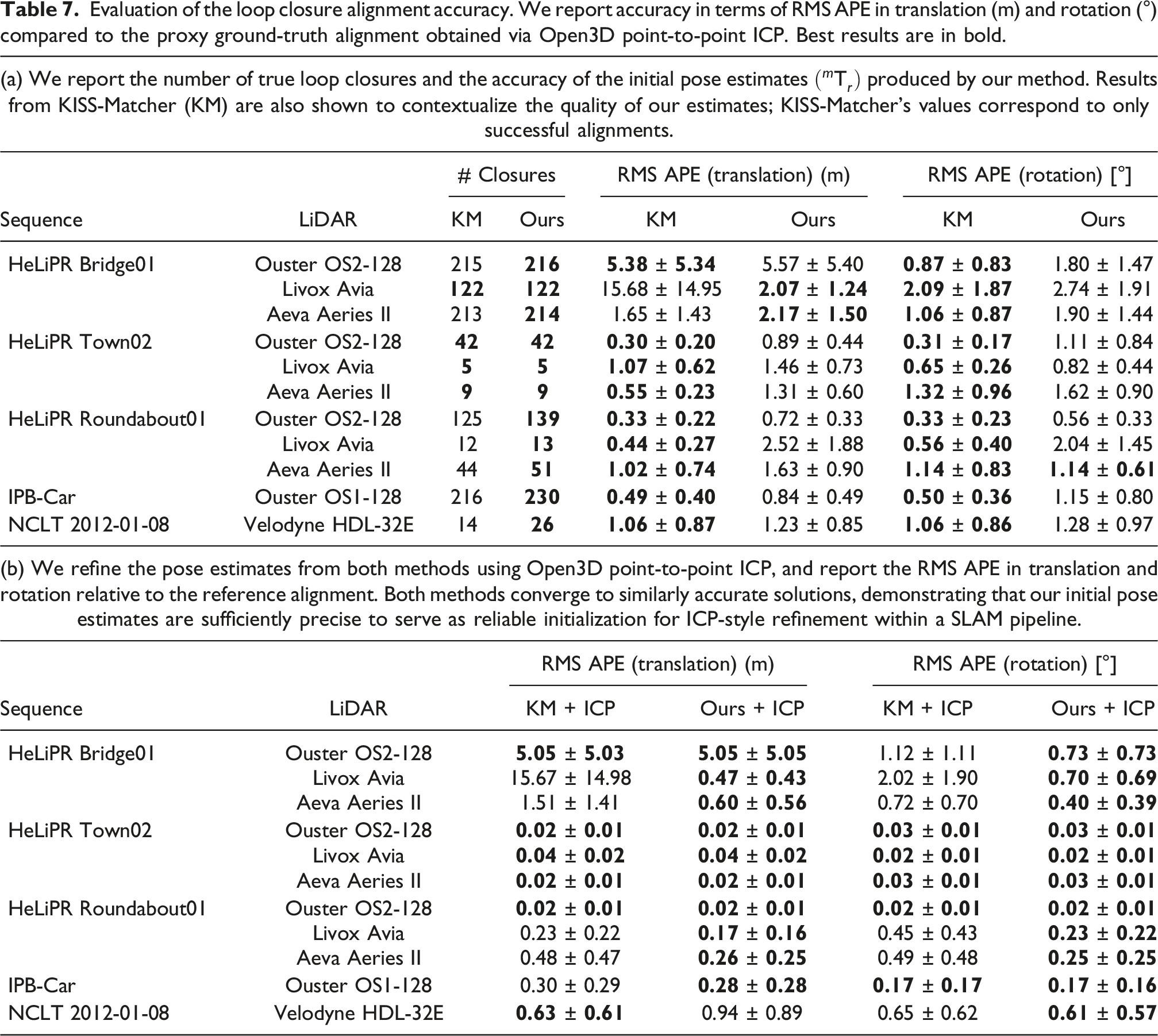
We also compare our method to KISS-Matcher by Lim et al. (2025) (KM), a state-of-the-art global point cloud registration method based on 3D features. For KISS-Matcher, we report the number of loop closures it successfully aligns (i.e., more than five inliers) and compute the corresponding RMS error metrics with respect to the reference alignment. We include this comparison not as a competing baseline, but to contextualize the quality of our initial alignment, and demonstrate how close our pose estimates are to those produced by a dedicated global registration system.
As shown in Table 7, KISS-Matcher, a technique designed to globally register point clouds, achieves better alignment accuracy across most sequences. This is expected as KISS-Matcher computes 3D features from the 3D point cloud and estimates the pose using a maximally consistent correspondence set. In contrast, our method combines 2D feature-based pose estimates with the approximate ground alignment estimates to get a complete 3D pose. Despite this fundamental difference, our RMS APE values remain within a few decimeters in translation and a couple of degrees in rotation compared to those of KISS-Matcher. Notably, KISS-Matcher performs worse than our method on the HeLiPR Bridge01 sequence because it lacks an explicit mechanism to handle perceptual aliasing during alignment.
To further demonstrate that our pose estimates are well-suited as initialization for a fine ICP-style alignment stage within a SLAM system, we explicitly run a point-to-point ICP refinement using Open3D, initialized with the pose estimates from our method as well as KISS-Matcher. The results in Table 7b show that both methods converge to solutions that are similarly accurate, and close to the reference alignment.
Our refined results also outperform KISS-Matcher on several sequences. The apparent performance inversion between KISS-Matcher and our pose estimation accuracy before and after ICP refinement may seem counterintuitive at first. A plausible explanation lies in the non-linear least-squares optimization underlying the ICP algorithm, which is sensitive to initialization and can converge to different local minima depending on the initial pose estimate.
Furthermore, two local maps generated from the same location using LiDAR odometry will generally not align perfectly, as they accumulate different amounts of drift and may contain artifacts due to imperfect scan deskewing. This could also lead to a different convergence for different initializations. It is also important to note that the discrepancy in performance between the two methods in Table 7b is, in most cases, on the order of only a few centimeters. The overall trend is that both methods converge to similarly accurate solutions after ICP refinement; therefore, we make no claims about the superiority of one method over the other in terms of final alignment accuracy.
Overall, these results support our fifth claim that the proposed approach yields accurate and complete 3D rigid-body transforms that align detected loop closures and are sufficiently precise to serve as initial guesses for fine-grained ICP-style registration within a SLAM back-end.
5.6. Multi-map alignment
This final experiment evaluates our pipeline’s ability to detect loop closures between the Riverside03 sequence and three KAIST sequences from the MulRan dataset. Although these trajectories share only minimal spatial overlap, it is sufficient to align the two scenes. These sequences also vary in temporal separation, with revisits ranging from the same day to a few months apart.
We first compare our method against baseline approaches using the precision-recall curves shown in Figure 17. Our approach consistently outperforms the baselines, achieving the highest recall while maintaining 100% precision across all three cases. Most other methods, except Scan Context, struggle in this challenging setting, with precision often falling below 50%. Precision-recall curves of our approach and state-of-the-art baselines for loop closure detection across sequences from the MulRan dataset with limited overlap.
Next, we compute the optimized trajectory for each sequence using in-session loop closure constraints detected by our method, followed by an additional pose-graph optimization step to align these optimized sequences across sessions using the inter-session closures identified by our pipeline.
We show in Figure 18 the final aligned trajectories and corresponding local maps, illustrating the successful alignment in the overlapping region. We report the precision, recall, and F1 scores for the inter-session loop closures in Table 8, using the default parameters detailed in Section 4.2. Despite the limited overlap, our method achieves perfect precision in all cases. We align three KAIST sequences to the Riverside03 sequence from the MulRan dataset using our loop closure pipeline. Despite the minimal spatial overlap, highlighted by the dashed rectangle, our approach accurately detects loop closures and aligns the corresponding local maps. Precision, recall, and F1 score for multi-session loop closures between the Riverside03 and KAIST sequences from the MulRan dataset. We report the RMS error in the overlap between aligned local maps using our pose estimate 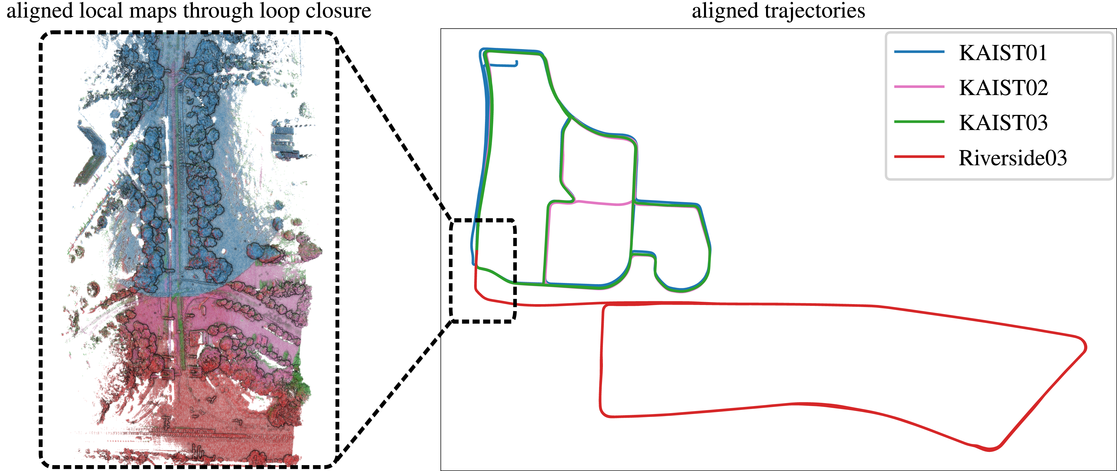
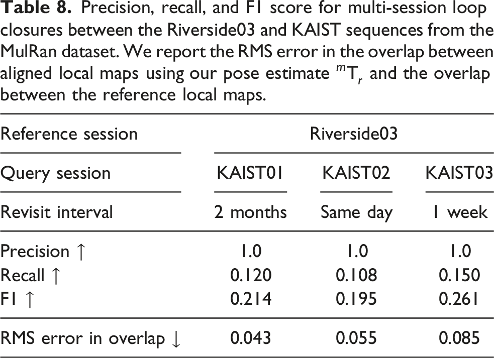
To assess the quality of the predicted alignment transformation
Additionally, we perform a similar cross-session multi-map alignment between the two self-recorded datasets, IPB-Car and IPB-Backpack, captured with different LiDAR sensors mounted on separate mobile platforms. These sequences exhibit varying motion dynamics and sensor configurations but still contain overlapping regions. We show the resulting aligned trajectories and detected loop closures in Figure 19. An example of loop closures detected between two sequences recorded with different LiDAR sensor platforms with a revisit interval of 2 weeks. In blue is the IPB-Backpack sequence, recorded on the campus of the University of Bonn with a Hesai Pandar-128 LiDAR mounted on a backpack. In red is the IPB-Car sequence, recorded in the city of Bonn with an Ouster OS1-128 LiDAR. Both trajectories were individually optimized through a pose-graph with in-session loop closure constraints obtained from our pipeline. We used our loop closure pipeline to detect inter-session loop closures between these two sequences, which have little overlap, and aligned the two trajectories using the multi-session loop closure constraints. The overlapping areas are highlighted by small rectangles, and the corresponding loop closure from these areas is shown in the enlarged rectangles, respectively.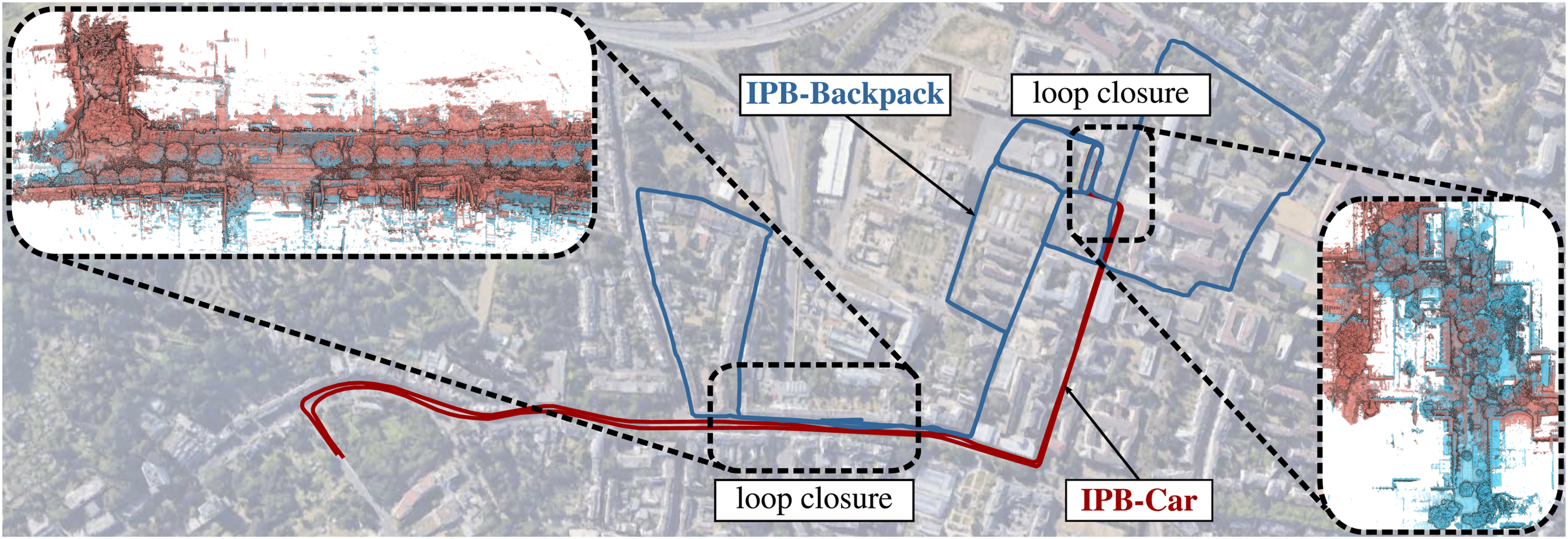
This experiment supports our final claim that our approach can successfully detect and align loop closures in challenging scenarios with little overlap. This capability is critical for tasks such as multi-robot map alignment, collaborative mapping, and long-term change detection.
5.7. Runtime evaluation of our approach
Runtime evaluation of our approach. We report the mean and standard deviation of the execution times for each key component of our pipeline.
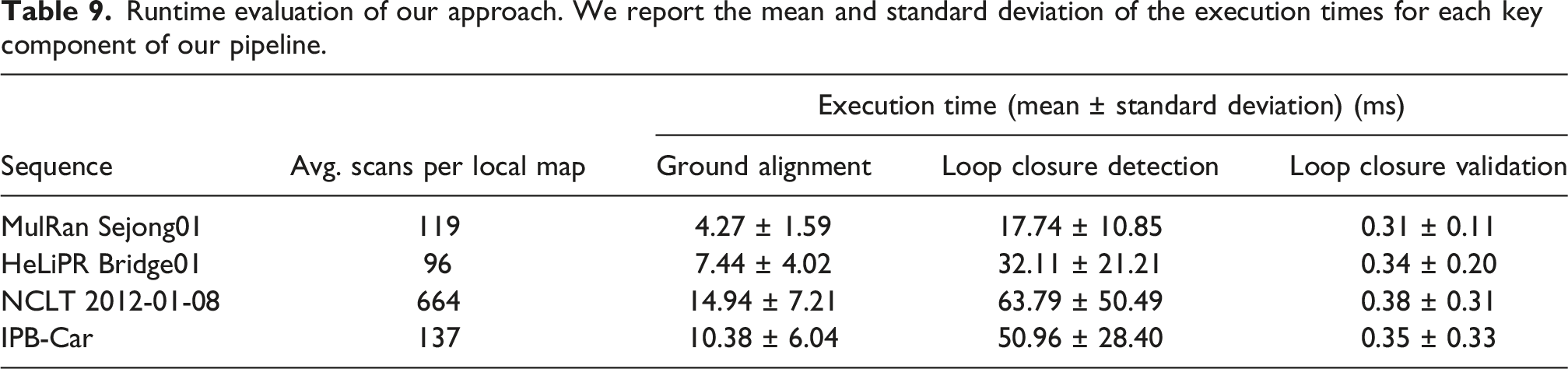
Average runtime evaluation of all the baselines. We report the average number of frames processed per second (FPS) for each baseline on three sequences with dense, 360° FoV LiDARs.
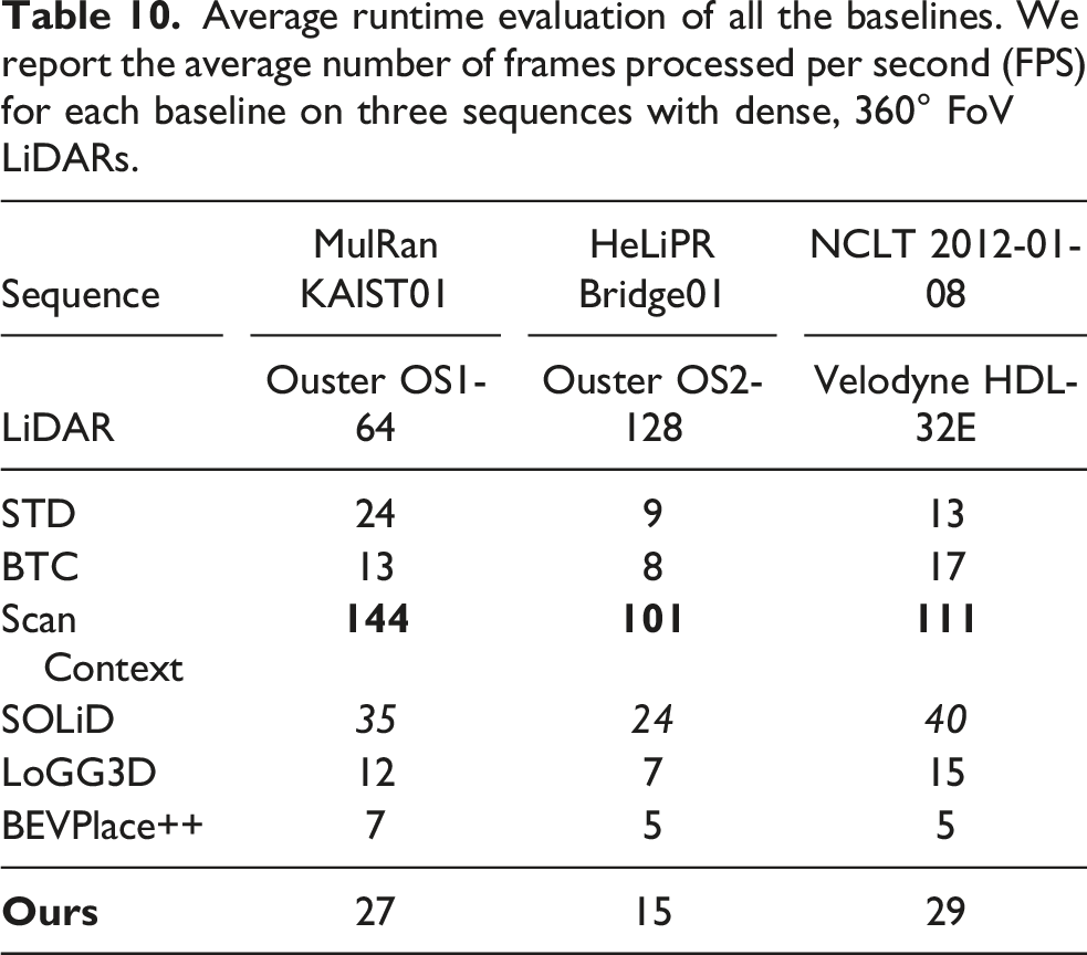
Overall, our approach achieves a favorable balance between speed and effectiveness, outperforming most conventional baselines while remaining significantly faster than other local map-based and learning-based methods, consistently maintaining processing speeds above the sensor frame rate.
In summary, the experiments presented above support all our claims and showcase the applicability of our approach across various scenarios. The first experiment shows the robustness of our approach to various scanning patterns, FoVs, and resolutions of the LiDAR sensor. The second experiment illustrates the applicability of our approach to detect loop closures between multiple sessions with short-term and long-term revisits through the same environment. The two subsequent experimental evaluations support the newly proposed modules in our loop closure pipeline. We show that our approach can be used on LiDAR platforms with non-planar motion and is also robust toward perceptual aliasing. The fifth experiment confirms that our pipeline produces accurate and complete 3D pose estimates for aligning loop closures. We further demonstrate that our approach can align multiple trajectories with minimal physical scene overlap. Finally, we show that our pipeline can efficiently operate above sensor frame rates, even on dense 3D LiDAR sensors.
6. Limitations
Our approach demonstrates robustness across multiple datasets, but it has certain limitations. The pipeline relies on locally consistent LiDAR odometry to generate local maps, which constitutes its most critical limitation. When the scan matching algorithm produces degenerate maps, loop closure performance also degrades. Incorporating more robust odometry that fuses inertial or visual data with LiDAR scans can help alleviate this limitation.
The method also depends on consistent ground plane detection for BEV projection, which may not hold in cluttered indoor, forested, or off-road scenarios. In such environments, approaches tailored to specific settings, such as ForestLPR (Shen et al., 2025), perform better. For aerial data, the density-preserving BEV projection can undersample vertical structures; a maximum-height BEV may provide a stronger alternative.
Although our method consistently performs better than existing baselines in intra-session and inter-session scenarios, inter-LiDAR scenarios remain challenging. Opposite-direction revisits with low-FoV LiDAR sensors, such as Livox Avia and Aeva Aeries II, are particularly difficult due to limited scene overlap, even after aggregation into local maps.
In summary, our method performs robustly across diverse urban datasets but is constrained by odometry quality, assumptions of a detectable ground plane, and reduced recall in the inter-LiDAR loop closure detection. Addressing these limitations will broaden its applicability to more diverse environments.
7. Conclusion
In this paper, we present a novel and robust approach to detect loop closures for LiDAR-based SLAM and provide 3D alignments between the detected closures. Our method leverages a density-preserving bird’s-eye-view projection of local maps generated from local odometry estimates. We use the local ground plane as a common reference plane across revisits and align the local maps such that the ground plane coincides with the xy-plane of the local map’s reference frame. This ensures a consistent BEV representation across diverse mobile platforms with varying LiDAR motion profiles. We extract ORB feature descriptors on these BEV projections and apply a self-similarity pruning strategy to reduce incorrect closures in repetitive environments.
We implement and extensively evaluate our approach on several public and self-recorded datasets featuring different LiDAR sensors mounted on various mobile platforms. We compare our method with state-of-the-art baselines and demonstrate its effectiveness in detecting loop closures in diverse urban settings across LiDAR sensors with different scanning patterns and fields of view. Furthermore, we illustrate the capability of our approach to detect long-term loop closures across multiple sessions. Finally, our runtime evaluations indicate the real-time feasibility of our approach.
To facilitate further research on place recognition and loop closure detection in LiDAR-SLAM, we release our software as open-source.
Supplemental material
Footnotes
Funding
The authors disclosed receipt of the following financial support for the research, authorship, and/or publication of this article: This work has partially been funded by the Deutsche Forschungsgemeinschaft (DFG, German Research Foundation) under Germany’s Excellence Strategy, EXC-2070 – 390732324 – PhenoRob, by the Deutsche Forschungsgemeinschaft (DFG, German Research Foundation) under STA 1051/5-1 – AID4Crops within the FOR 5351, by the European Union’s Horizon Europe research and innovation programme under grant agreement No 101070405 – DigiForest, and by the German Federal Ministry of Research, Technology and Space (BMFTR) under the Robotics Institute Germany (RIG).
Declaration of conflicting interests
The authors declared no potential conflicts of interest with respect to the research, authorship, and/or publication of this article.
Supplemental material
Supplemental material for this article is available online.
References
Supplementary Material
Please find the following supplemental material available below.
For Open Access articles published under a Creative Commons License, all supplemental material carries the same license as the article it is associated with.
For non-Open Access articles published, all supplemental material carries a non-exclusive license, and permission requests for re-use of supplemental material or any part of supplemental material shall be sent directly to the copyright owner as specified in the copyright notice associated with the article.