Actuator fault recovery with deep reinforcement learning in a linear model-based control framework: Application to a physical AUV

Abstract

Actuator faults in autonomous mobile robotic systems pose significant challenges, especially in unpredictable environments where system reliability is paramount. Fault tolerant control (FTC) strategies, particularly those leveraging actuator redundancy, have been explored to address these issues. However, traditional methods commonly rely on explicit fault diagnosis, which can be resource-intensive and challenging to implement accurately. This paper introduces a novel approach that combines deep reinforcement learning (DRL) with a linearised optimal model-based controller to achieve actuator fault recovery without explicit fault diagnosis. The integration of DRL within a model-based controller framework enhances system stability and fault recovery capabilities. The chosen application platform for this study is an autonomous underwater vehicle (AUV), where the partial or total failure of a mission critical component such as a thruster could jeopardise the success of the mission and potentially render the vehicle unrecoverable in the event of a fault. In this application case, a linear quadratic regulator (LQR) controller is employed as the model-based controller, while the soft actor-critic (SAC) algorithm is used as the DRL component to handle fault recovery. The DRL model is trained and evaluated in simulation before being directly applied to the physical AUV. The proposed method’s effectiveness is demonstrated through comparisons with a standard LQR controller, a conventional adaptive LQR controller and the proposed hybrid LQR-SAC controller. The results indicate that the LQR-SAC controller outperforms the standard and conventional adaptive LQR controllers in maintaining system performance under fault conditions, achieving a significant reduction in trajectory tracking error on a physical AUV.

Keywords

deep reinforcement learning actuator faults fault tolerance control reallocation adaptive control autonomous underwater vehicle sim-to-real application

1. Introduction

Autonomous mobile robotic systems, such as self-driving cars and drones, increasingly support commercial and defence applications. Their ability to perform precise and complex tasks depends on actuators, whose faults – ranging from partial efficiency loss to complete failure – can jeopardise system stability and performance. This challenge is particularly critical in unpredictable environments, where reliability is essential. In the literature, the set of control strategies enabling a system to overcome a fault situation is called fault tolerant control (FTC) (Patton, 2021). The focus here is on FTC strategies for actuator faults in autonomous mobile robotic systems. The consequences of actuator faults and the existing FTC strategies are wide-ranging and depend on each system and environment, which is why it is necessary to establish the following working assumptions.

Assumption 1: The system remains controllable despite actuator faults. This means that the system retains the ability to move from one state to another within a finite time, provided it has sufficient numbers of additional independent actuators to influence all controllable states of the system.

Assumption 2: There are no other external disturbances during the mission. As the focus is on actuator faults, it is assumed for purposes of simplification that the dynamic system is not subject to environmental disturbances, such as waves or sea currents.

Under these assumptions, existing FTC strategies in the literature rely on actuator redundancy to overcome faults (Amin and Hasan, 2019; Jin et al., 2017). This redundancy allows the system to redistribute control efforts among the remaining functioning actuators, ensuring that the desired performance is maintained despite the presence of faults.

Even if the FTC area of research is undergoing continuous development, key attributes of fault-tolerant controllers have been identified, based on a review of several studies in the literature (Abbaspour et al., 2020; Noura et al., 2009; Patton, 2021).

Key attributes of the controller include optimal recovery performance, ensuring the best achievable system behaviour despite fault-induced constraints, and stability, which guarantees the system returns to equilibrium after disturbances (Atassi and Khalil, 1999). Adaptability, that is, the extent of the range of faults that the FTC strategy is capable of handling, is also essential for handling a wide range of actuator faults, especially when multiple actuators can be faulty (De Kleer and Williams, 1987). Additionally, generalisability allows the system to manage unforeseen faults, that is, it allows the system to manage faults it was not specifically configured to overcome. Finally, resource efficiency is crucial for many autonomous systems that operate in environments where resources are limited, such as underwater or space exploration. In the case of actuator faults, the FTC strategy must be performed in real-time, potentially with the constrained computational power and energy resources available on autonomous mobile systems.

FTC strategies have been widely explored over the years, as dynamic systems have grown in complexity and their reliability has become increasingly important. One of the earlier approaches is passive FTC (Benosman, 2011), a method designed to manage a certain range of faults without the need for real-time adjustments (Wang et al., 2014). Its reliability, however, diminishes significantly for faults beyond the design basis (Yu and Jiang, 2015), and it is not optimal for all design scenarios, often forcing a trade-off between robustness and system performance (Saied et al., 2020). For this reason, adaptive techniques are generally preferred for actuator fault recovery.

Direct adaptive FTC strategies (Ioannou and Sun, 2012) aim to overcome faults by directly adjusting the controller’s gains. In some cases, adjusting the controller’s gains in an actuator fault situation can cause actuator saturation and worsen the system’s performance due to the geometric configuration of the actuators (Tao et al., 2013).

Indirect adaptive FTC methods (Gao et al., 2015) propose a more nuanced control adjustment by using control reallocation (Ijaz et al., 2023), with recent developments focusing on constrained strategies (Naderi et al., 2019). Control reallocation is a process involving the redistribution of the controller outputs among the actuators to maintain system performance and stability despite actuator faults. This is a direct and efficient method to overcome actuator faults, but it is heavily dependent on an explicit fault diagnosis (Gao et al., 2015), which involves identifying the type and extent of a fault. Actuator redundancy via control reallocation and explicit fault diagnosis address different aspects of FTC: redundancy enables redistribution of control, while diagnosis provides the information needed to guide this redistribution.

Explicit fault diagnosis can be performed using two approaches: one based on prior knowledge of faults and their effects on system behaviour (Patton, 1994), and another based on online fault estimation (van Den Bosch and Van der Klauw, 2020). Among the many challenges of explicit fault diagnosis, state estimation under fault conditions is one of the most critical, as accurate information on the system state is essential for identifying and compensating faults. The effectiveness of the approach based on prior knowledge of faults, in terms of adaptability and generalisability, is constrained by the extent of available knowledge, which becomes increasingly demanding as the number of possible faults grows and as actuator geometries become more complex, introducing strong couplings between multiple degrees of freedom. The latter approach, which uses embedded optimisation for real-time parameter estimation (Poli et al., 2007), can be computationally intensive, posing challenges for embedded systems with limited computing power or when rapid fault response is required.

This is why this work focuses on systems where explicit fault diagnosis is particularly difficult to obtain either due to the complexity of actuator geometry, or due to limited onboard computational resources preventing real-time optimisation-based estimation. In this context, the following question is addressed: how can these limitations of explicit fault diagnosis be overcome to improve fault recovery in autonomous dynamic systems?

To overcome the drawbacks of explicit fault diagnosis methods, data-driven approaches have been explored, due to their ability to handle complex, high-dimensional data and to generalise across unseen fault scenarios without relying on exhaustive fault modelling. Among these, deep reinforcement learning (DRL) (Sutton and Barto, 2018) has emerged as a particularly promising direction.

DRL is a subset of machine learning which involves training an agent to make decisions by rewarding it for desirable actions and penalising it for undesirable ones. This training process enables the agent to learn complex policies mapping states to actions directly from raw sensory inputs, making DRL suitable for dynamic systems evolving in uncertain environments.

An end-to-end DRL-based actuator fault-tolerant control has been presented in our previous work (Lagattu et al., 2024). Although the effectiveness of the end-to-end DRL-based approach has been demonstrated, a significant drawback of employing this method is the complexity in guaranteeing system stability. The stability challenge arises from the integration of deep neural networks (DNNs) (François-Lavet et al., 2018), which, due to their inherent non-linearity, makes it difficult to predict the system behaviour. The unpredictability and lack of transparency of end-to-end DRL-based techniques are highlighted in the work of Dulac-Arnold et al. (2020). Besides, Chaffre et al. (2021) compared end-to-end and model-based approaches, and showed that despite achieving similar average performance, the purely end-to-end strategy suffers from major drawbacks in terms of stability and variance. Another well-known drawback of end-to-end methods is their high sample complexity, which can make training prohibitively costly in terms of data and time (Dulac-Arnold et al., 2020).

In order to bring stability to an end-to-end DRL controller and reduce the amount of data required for learning, a solution is to combine optimal model-based control methods with DRL techniques. This approach leverages the strengths of optimal model-based controllers in providing stable control for known system dynamics, while using the adaptive capabilities of DRL to handle unknown dynamics that may arise during operation (Chaffre, 2023; Lewis et al., 2012b; Yoo et al., 2021).

This paper introduces a novel FTC strategy to overcome actuator faults in autonomous mobile robots by integrating DRL within an optimal linear model-based control framework.

The main novelty of this approach is that it enables control reallocation for actuator fault recovery without relying on explicit fault diagnosis. Instead, a DRL model is trained to compensate for the effects of faults through interaction with the environment. This allows the system to adapt its behaviour in the presence of faults, while the linear model-based controller aims to maintain consistent performance.

Following an initial section discussing related work, this proposed approach will be set out in Section 3. The chosen application domain is the autonomous underwater vehicle (AUV), as described in Section 4. Although underwater vehicles are governed by coupled nonlinear dynamics, the controller proposed in this work was designed from a linearisation of the nonlinear model around a nominal operating trajectory, providing local closed-loop stability guarantees for the linearised system. In this application case, the linear quadratic regulator (LQR) (Benner, 2006) controller was chosen as the model-based controller and the soft actor-critic (SAC) (Haarnoja et al., 2018b) algorithm was used as the DRL component of the proposed controller.

The application case is restricted to planar motion, where the four horizontal thrusters provide an overactuated configuration. This restriction allows to isolate the effects of actuator faults from other dynamic effects and environmental disturbances, in order to clearly assess the contribution of the DRL-based control reallocation strategy.

The proposed controller was evaluated both in simulation and on a real BlueROV2 Heavy platform (Inc, 2017), and compared with two baseline controllers: a standard LQR controller with fixed gains and an adaptive LQR controller that adjusts the weighting matrix Q online. The simulation was conducted using the UUV Simulator package (Manhães et al., 2016) in GAZEBO (Koenig and Howard, 2004). The approach was tested on a physical BlueROV2 Heavy in an experimental tank at Flinders University. A detailed presentation and analysis of the results is provided in Section 5.

2. Related work

In this section, we first outline key concepts of DRL and then examine how DRL has been combined with model-based control in the literature to address challenges in the control of autonomous dynamic systems.

2.1. Deep reinforcement learning

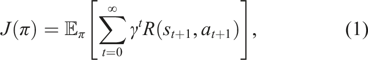
DRL is a machine learning approach that combines reinforcement learning (Sutton and Barto, 2018) and DNNs (François-Lavet et al., 2018). The fundamental framework for reinforcement learning is the Markov decision process (MDP) (Puterman, 1990). An MDP represents a mathematical framework used to describe an environment in which an agent makes decisions under uncertainty. A MDP is defined by a tuple (S, A, T, R), where S represents a set of states, A is a set of actions, T(s_t, a_t, s_t+1) defines the state transition probabilities given the current state s_t and action a_t, and R(s_t, a_t) is the reward function that the agent receives for moving from state s_t to s_t+1 by performing action a_t. The action selection process is described through what is known as the policy π: S → A. It serves as a mapping from the state s_t to action a_t and can be of a stochastic nature. The fundamental assumption in an MDP is the first-order Markov property, which states that the future state s_t+1 is conditionally independent from all preceding states except the current state s_t.

In an MDP, a reinforcement learning agent interacts with its environment to learn optimal action selection strategy π. The goal for the reinforcement learning agent is to maximise the expected cumulative reward expressed in the objective function J(π):

J (π) = E_{π} [\sum_{t = 0}^{\infty} γ^{t} R (s_{t + 1}, a_{t + 1})],

(1)

where γ is the discount factor that balances future rewards,

E [.]

is the expectation operator and π is the policy. The agent aims to find the optimal policy (π*) that maximises this expected return.

During the training phase, the DRL agent learns to make decisions by interacting with its environment through a series of episodes where at each step, the agent takes an action and receives feedback from the environment in the form of a reward.

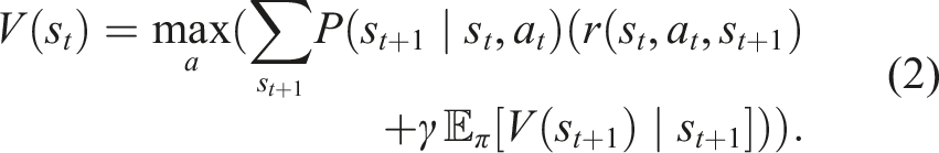
DRL combines these principles of reinforcement learning with DNNs. DRL leverages DNNs to approximate the policy and value functions. The policy network π_θ(a_t|s_t) outputs the probability distribution of actions a_t given state s_t, while the value network V(s_t) estimates the expected cumulative return from state s_t. The policy is optimised by gradient ascent, and the value function is updated through the Bellman equation:

\begin{aligned} V (s_{t}) = \max_{a} (\sum_{s_{t + 1}} P (s_{t + 1} ∣ s_{t}, a_{t}) (r (s_{t}, a_{t}, s_{t + 1}) \\ + γ E_{π} [V (s_{t + 1}) ∣ s_{t + 1}])) . \end{aligned}

(2)

Using DRL to control autonomous dynamic systems has several advantages. DRL enables fault tolerance without any need for explicit fault diagnosis by directly controlling the dynamic system, based on training experience and observation of the system’s behaviour (Lagattu et al., 2024). DRL-based FTC strategies perform an implicit fault diagnosis as the adjustments made by the DRL model to the control system are based on the observation of the faulty system’s behaviour, which reflects the type and extent of the fault. The control input of the system, taken according to the DRL model policy, is based on the similarities between the observed behaviour and the fault situations experienced during training.

DRL is also particularly well suited for managing various actuator faults without explicit fault diagnosis due to its capacity for adaptation and generalisation (Sutton and Barto, 2018). DRL’s adaptability stems from training across diverse fault situations, enabling it to develop a rich knowledge base. The architecture of neural networks (NNs) enables a wide range of information to be processed, facilitating the learning of different situations and the associated responses (Ahmadzadeh et al., 2014; Fei et al., 2020; Hadi et al., 2022). In addition, DRL has a capacity for generalisation, which is particularly suitable in the case of actuator faults: it has the potential to recover from faults it has not encountered during training, provided they are sufficiently similar to those seen during learning, due to the fact that NNs are universal function approximators. The DRL agent uses these approximators whose effectiveness depends on the similarity between the current situation and the situations encountered in training (Kohl and Miikkulainen, 2009). Another advantage is that once offline-trained, DRL-based FTC methods have a low computational demand and are suitable for embedding.

Now that the key concepts of DRL have been discussed, we shift our focus to how DRL has been combined with model-based control approaches in the literature, to provide insights into designing the hybrid approach proposed in this article.

2.2. Combined DRL and model-based control

The integration of DRL and model-based control methods has been investigated, primarily to enhance adaptability and stability in dynamic systems facing system uncertainties or external disturbances such as wind or currents (Rizvi and Lin, 2019; Yaghmaie et al., 2022). This combination leverages the adaptive capabilities of DRL and the robustness of model-based controllers to improve performance in unpredictable environments.

One popular approach involves using DRL to optimise the gains of controllers such as proportional–integral–derivative (PID) controller (Johnson and Moradi, 2005) and LQR. For instance, several studies have shown that DRL can efficiently learn PID controller gains, allowing improved adaptability to system changes (Clement et al., 2021; Sedighizadeh and Rezazadeh, 2008; Shuprajhaa et al., 2022; Wang et al., 2007). Notably, in the work of Clement et al. (2021), the SAC algorithm with automatic temperature adjustment was used to adapt PID gains for an AUV, demonstrating effectiveness in both simulated and physical systems. Similarly, DRL has been employed to optimise LQR controllers, with results showing that this hybrid approach not only enhances performance under uncertainty but also reduces computational complexity by operating on a lower-dimensional action space (Bradtke, 1992; Görges, 2019; Rizvi and Lin, 2019; Yaghmaie et al., 2022).

To ensure stability in these hybrid controllers, constraints on adapted parameters or Lyapunov-based stability criteria (Lyapunov, 1992) are commonly used. Lyapunov-based methods ensure stability by constraining the adaptations introduced by the DRL agent (Kohler et al., 2022), such as modifications of controller gains or elements of the control allocation matrix. A candidate Lyapunov function V(x) is defined to represent the system’s energy, and parameter updates are accepted only if they satisfy $\dot{V} (x) \leq 0$ , thereby guaranteeing closed-loop stability (Rizvi and Lin, 2023).

Although most hybrid methods focus on addressing uncertainties or disturbances, a few studies have explored their use for actuator fault recovery. For example, Bhan et al. (2021) combined DRL with PID control to recover performance after actuator faults. Their approach used filters such as the unscented Kalman filter (Wan and Van Der Merwe, 2001) to estimate fault parameters, which were then used by the DRL agent to adapt PID gains dynamically. This method was demonstrated on an octocopter for trajectory tracking, effectively recovering performance despite faults. However, this approach relies on the accuracy of an explicit fault diagnosis, which can be challenging to obtain due to the complexity of identifying the exact nature and extent of faults in real-time.

Another approach, proposed in the work of Ma and Peng (2021), combined DRL with an LQR-like controller. By introducing the integral of the tracking error as an augmented state, the controller adapted to faults and uncertainties without requiring prior knowledge of system dynamics. The authors demonstrated stability through boundedness of the closed-loop system and showed fault accommodation in numerical simulations of an aircraft. However, this method also employed a direct adaptive control strategy, with real-time modifications to the LQR gains, which does not allow performing a direct redistribution of forces among the actuators taking into account the geometric configuration of the actuators in a fault situation.

In our previous work (Lagattu et al., 2025a), control reallocation was handled by a DRL model acting on top of a standard PID controller with fixed gains. However, since this controller was not model-based, no formal guarantees on closed-loop stability could be provided.

The mentioned challenges of existing methods highlight the need for a model-based fault recovery strategy that does not rely on explicit fault diagnosis and is capable of reallocating control forces among actuators while accounting for their physical configuration. The next section introduces a new approach that combines DRL with a model-based controller to achieve control reallocation for actuator fault recovery without the need for explicit fault diagnosis.

3. Combining DRL and model-based control for actuator fault recovery

This section describes the structure of our proposed controller aiming to overcome actuator faults without the need for explicit fault diagnosis. Explicit fault diagnosis methods are powerful and well established in the literature, but their applicability can be reduced in systems with complex actuator geometries or limited onboard computational resources (Zhang et al., 2025). In such situations, the proposed hybrid approach provides an alternative method by bypassing explicit fault diagnosis while retaining stability guarantees. The proposed method is a hybrid strategy: the model-based controller ensures stability, while the DRL component brings adaptability by reallocating control forces without explicit diagnosis. In this work, the controller is designed using a linearised representation of the nonlinear system around a nominal operating trajectory. The stability guarantees derived in this section therefore apply locally to the linearised closed-loop system. The proposed method is applicable to autonomous dynamic systems equipped with actuators operating in the continuous time domain and satisfying the assumptions outlined in the introduction.

3.1. Problem modelling

Let’s consider the control structure of the dynamic system presented in Figure 1 (Franklin et al., 2002), where w_ref is the reference vector, $τ \in R^{n}$ is the control output vector containing n forces, $u \in R^{r}$ is the actuator input vector for r actuators, $T \in R^{r}$ is the actuator output vector, and y_obs is the observation vector, defined within the earth-fixed coordinate frame.

Figure 1.

Control law and control allocation scheme.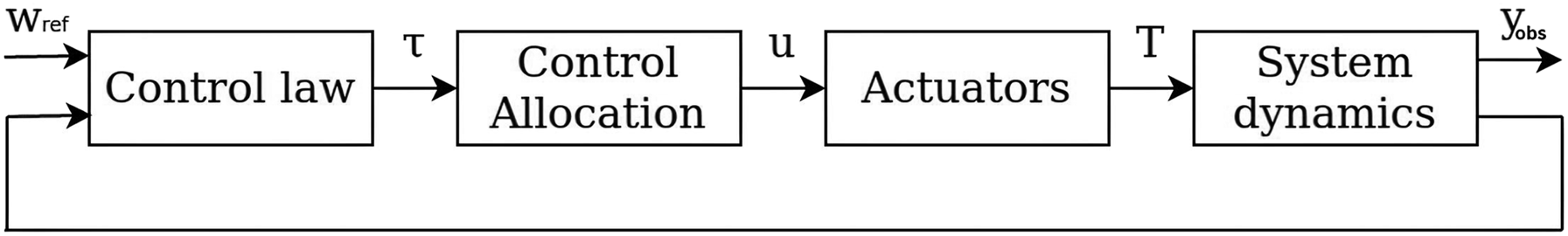

The system is controlled by a model-based controller which relies on the following evolution equation (Brosilow and Joseph, 2002):

\dot{x} (t) = A x (t) + B τ (t),

(3)

where x(t) is the state vector, which represents the internal states of the system at time t, A is the system matrix which defines how the current state x(t) evolves over time based on its current value, and B is the input matrix which determines how the control output at time t, τ (t), affects the change in the state x(t).

Control allocation refers to the process of transforming control outputs into actuator inputs by means of a control allocation matrix (CAM) (Johansen and Fossen, 2013). It enables the achievement of the desired control objectives while considering the characteristics of each actuator. The relationship between the control outputs and the actuator inputs can be expressed as:

τ (t) = H u (t),

(4)

where H denotes the CAM of dimensions (n, r).

The system under study is overactuated, meaning that H is full rank (i.e., rank equal to n) and r > n. To determine the actuator input vector that produces the desired control outputs, the Moore-Penrose pseudoinverse is used (Barata and Hussein, 2012):

u (t) = H^{T} {(H H^{T})}^{- 1} τ (t) .

(5)

Actuator saturation is enforced by bounding each control input within its admissible limits. The computed control commands are therefore clipped to satisfy the physical actuator constraints.

The occurrence of actuator faults, whether total or partial, affects the actuator output vector, resulting in a behaviour that deviates from the intended one. The objective of the proposed approach is to maintain control of the dynamic system despite an actuator fault, allowing the system to follow the desired trajectory.

In the case of an actuator fault, the CAM is no longer valid, as the distribution of forces among the actuators required to achieve the desired motion changes depending on the fault and the geometric configuration of the actuators. The faulty system is assumed to remain controllable (Assumption 1), meaning that an appropriate CAM exists for the faulty system’s configuration. Therefore, updating the CAM, that is, performing control reallocation, is an efficient way to recover from actuator faults. The challenge is to achieve this control reallocation while preserving the stable structure of the model-based controller. The next section addresses this challenge by presenting the proposed controller structure.

3.2. Proposed controller structure

The goal of the proposed controller is to use the adaptability of DRL to overcome actuator faults without any explicit fault diagnosis, in a model-based control framework.

In the proposed approach, DRL is used only when abnormal behaviour is detected. This ensures optimal control under normal conditions, where model-based controllers provide global stability and efficiency without adjustments. This selective use of DRL reduces the learning required by focusing only on actuator faults, enabling faster convergence with improved performance under fault conditions.

In order to avoid any bias during the training process, the DRL agent is trained offline only on fault scenarios. During the mission, DRL is activated upon abnormal behaviour with no further learning, ensuring real-time applicability. During normal operation, the DRL module remains inactive and control is fully governed by the model-based controller.

The detection of an abnormal behaviour relies on a binary indicator that flags deviations from expected behaviour, without performing explicit fault diagnosis. Given that the system state is assumed to be free from disturbances, fault detection is performed by comparing the desired and actual system states. If their difference exceeds a predefined threshold a fault is detected, triggering a DRL algorithm to update the CAM, as illustrated in Figure 2.

Figure 2.

Fault detection scheme.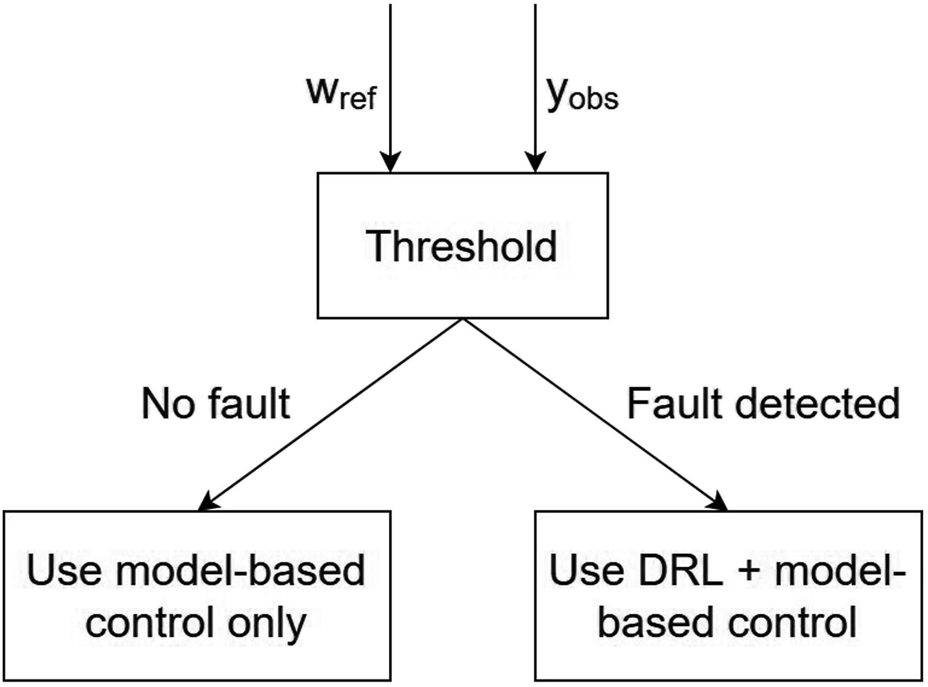

DRL is used to adjust the CAM in case of a fault situation. The DRL model input must provide sufficient information to infer actuator faults from the system’s behaviour and adjust its actions accordingly.

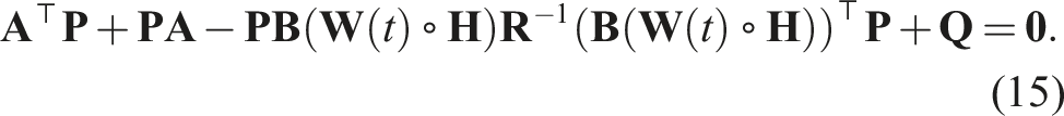
Furthermore, the proposed controller is not divided into two separate blocks with a control law and an allocation law, as commonly done (Franklin et al., 2002). In the proposed approach, the controller directly outputs the actuator inputs u, and the DRL model adjusts the CAM which is integrated in the control law equations (control reallocation) as shown in Figure 3.

Figure 3.

Proposed hybrid model-based/DRL controller scheme for actuator fault recovery.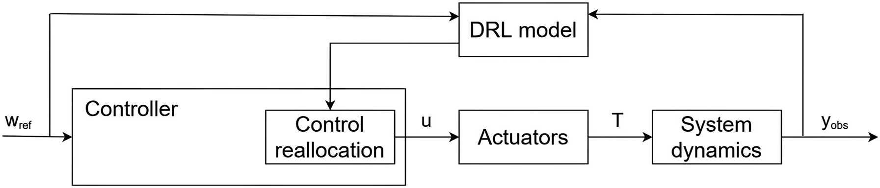

The next two sections focus respectively on the CAM adjustment with DRL and on the integration of the adjusted CAM in the model-based controller equations.

3.3. DRL-based control reallocation

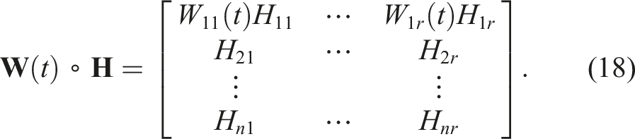
To adjust the CAM in order to redistribute the forces among the actuators, a weight matrix $W \in R^{n \times r}$ is introduced and defined such that, in the absence of faults, all its elements are equal to one. In the event of an actuator fault situation, the weight matrix is time-varying and updated by the DRL model. The control allocation equation becomes:

τ (t) = (W (t) ◦ H) u (t),

(6)

where the Hadamard product (Horn, 1990) W(t) ◦ H can be expressed as follows:

W (t) ◦ H = [\begin{matrix} W_{11} (t) H_{11} & W_{12} (t) H_{12} & \dots & W_{1 r} (t) H_{1 r} \\ W_{21} (t) H_{21} & W_{22} (t) H_{22} & \dots & W_{2 r} (t) H_{2 r} \\ W_{31} (t) H_{31} & W_{32} (t) H_{32} & \dots & W_{3 r} (t) H_{13r} \\ ⋮ & ⋮ & ⋮ & ⋱ \\ W_{n 1} (t) H_{n 1} & W_{n 2} (t) H_{n 2} & \dots & W_{n r} (t) H_{n r} \end{matrix}] .

(7)

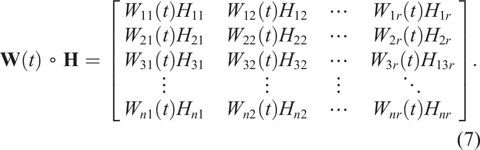
The objective of the proposed DRL-based control reallocation strategy is to determine appropriate coefficients in the weight matrix W(t) without any need for explicit fault diagnosis. This strategy also addresses the sample efficiency limitation of purely end-to-end DRL controllers: the DRL agent learns weight coefficients for the allocation matrix rather than producing direct actuator inputs, thereby reducing the action space and accelerating convergence.

In our proposed approach, the DRL agent’s action lies within the space of matrix W, which is constrained by the system’s acceptable value range. For each action taken, the environment provides feedback through the observation y_obs, determining the next state s_t+1 as follows:

s_{t + 1} = y_{obs} (t + 1) .

(8)

To ensure uniform treatment of all observations by the DRL model, y_obs undergoes normalisation (Sutton and Barto, 2018).

In the context of dynamic systems with actuators, deviations from the intended motion introduce translation and rotation errors. The corresponding normalised errors are denoted as e_T and e_R, respectively. These quantities are obtained by dividing the position and orientation errors by predefined maximum admissible values, ensuring dimensionless terms. The DRL model is trained by minimising these errors, which are derived from y_obs and w_ref, through the design of a reward function that penalises tracking deviations. In this work, the reward is defined as

r = - \exp (e_{T} + e_{R} + \dot{e_{T}} + \dot{e_{R}}),

(9)

The inclusion of the derivative terms penalises rapid variations in translational and rotational dynamics, promoting smoother system behaviour. To improve the robustness of the learned policy, environment randomisation is applied during training. The DRL agent is exposed to various actuator fault scenarios, allowing it to experience different fault conditions across episodes. This randomisation ensures that the agent does not overfit to a specific fault pattern and encourages the development of a more general control strategy capable of handling a wider range of actuator faults, while also improving the agent’s ability to adapt to real-world variations (Tobin et al., 2017).

The selection of the DRL algorithm is a critical aspect of the proposed method. Since the control reallocation strategy involves multiple continuous input and output variables, the chosen algorithm must efficiently handle continuous actions to enable smooth adjustments in response to actuator faults. Additionally, learning efficiency is essential, as practical constraints often limit the amount of available interaction data. The algorithm must therefore be sample-efficient to achieve high performance with minimal data. The choice of the DRL algorithm for our application case will be detailed in Section 4.

The following part outlines the incorporation of the adjusted CAM into the model-based control framework with the objective of ensuring stability.

3.4. Integration of the adjusted CAM in the model-based control framework

The proposed approach aims to perform control reallocation while maintaining the stability of the closed-loop. In control theory, including varying parameters in the state equations is essential for maintaining the stability of a varying-parameter controller (Mohammadpour and Scherer, 2012). This is why the adjusted CAM needs to be included in the state equations of the system.

To achieve this integration, we transform the standard evolution equation involving the control input τ of linear systems defined in equation (3) into a new evolution equation that incorporates the CAM adjusted by the weight matrix and the actuator input vector u, resulting in:

\dot{x} (t) = A x (t) + B (W (t) ◦ H) u (t) .

(10)

Hence, the model-based controller’s output is directly the actuator input vector. The augmented evolution equation implies that the proposed approach focuses on a class of model-based controllers characterised by a gain K that varies over time and can be determined as a function (denoted f) of the matrices A, B, and the adjusted CAM:

K (t) = f (A, B (W (t) ◦ H), Q_{1}, Q_{2}, \dots, Q_{n}),

(11)

where Q₁, Q₂, …, Q_n represent the weighting matrices of the model-based controller. The gain K is recalculated at each new adjustment of the CAM by the DRL model. Without this recalculation, relying only on the mapping of H would not suffice to guarantee closed-loop stability in the presence of actuator faults.

The actuator inputs are then calculated using the following relationship:

u (t) = - K (t) x (t) .

(12)

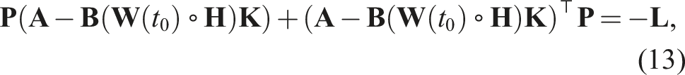
This transformation enables us to establish the local stability of the system by determining the eigenvalues of A − B(W ◦ H)K. More specifically, the stability can be established at a given time t₀ by finding a symmetric positive definite matrix P that satisfies the Lyapunov equation:

P (A - B (W (t_{0}) ◦ H) K) + {(A - B (W (t_{0}) ◦ H) K)}^{⊤} P = - L,

(13)

where L is a positive definite matrix. The existence of such a matrix P guarantees that the eigenvalues of A − B(W(t₀) ◦ H)K lie in the left half of the complex plane, indicating the asymptotic stability of the system at t = t₀ (Benner, 2006).

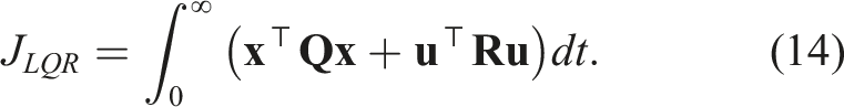
A classic model-based controller for linear systems is the LQR controller (Benner, 2006). This controller is widely used due to its ability to compute an optimal state-feedback control law by minimising the quadratic cost function:

J_{LQR} = \int_{0}^{\infty} (x^{⊤} Q x + u^{⊤} R u) d t .

(14)

The matrices Q and R are positive definite weighting matrices that define the relative importance of the state error and control effort, respectively. Several methods exist to identify appropriate values for Q and R. Optimisation-based techniques can be employed to adjust these matrices in order to meet specific performance criteria (Lewis et al., 2012a). In addition, evolutionary algorithms, such as particle swarm optimization (PSO) (Kennedy and Eberhart, 1995), have been used to automatically tune Q and R by searching for values that optimise predefined control objectives. PSO is based on a population of particles that iteratively update their positions in the search space by combining information from their own best solutions and the global best solution. Although efficient and widely applied, PSO is known to be sensitive to its hyperparameters, such as the inertia weight and acceleration coefficients, which strongly affect convergence behaviour (Clerc and Kennedy, 2002). To mitigate this sensitivity, adaptive strategies and alternative evolutionary algorithms, such as Genetic Algorithms (Sivanandam and Deepa, 2008), can also be considered.

For the proposed approach, we selected the LQR controller because of its effectiveness in optimally controlling linear systems and the straightforward establishment of its stability. At each CAM update, the gain K(t) is computed to ensure local stability, by solving the Riccati equation (Benner, 2006) which includes the adjusted CAM:

A^{⊤} P + P A - P B (W (t) ◦ H) R^{- 1} {(B (W (t) ◦ H))}^{⊤} P + Q = 0 .

(15)

For a given weight matrix, local stability can be guaranteed as described above. However, even if the outputs of the DRL model can be bounded to maintain safety limits, the unpredictable nature of DRL, due to the complexity of the neural networks, makes global stability challenging to achieve.

In order to approach global stability, a post-processing step can be added to the DRL model’s outputs. Variations in the values of the weight matrix can be mitigated using smoothing or regularisation techniques (Roberts and Mullis, 1987). In this way, the DRL outputs produce smaller and more continuous variations, which contribute to more stable control behaviour. Figure 4 shows the details of the proposed controller, with W_fil representing the filtered weights and $\hat{x}$ the estimated state of the system.

Figure 4.

Detailed proposed hybrid controller structure.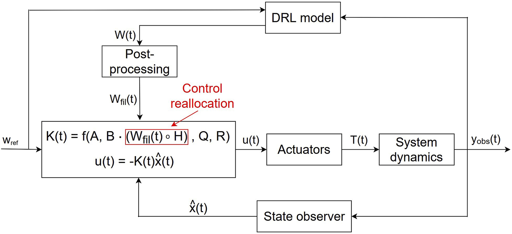

This proposed controller was applied to thruster faults in an AUV, as detailed in the next section.

4. Application case: Actuator faults in BlueROV2 Heavy

In this section, we present the practical application of the proposed controller on a BlueROV2 Heavy (BlueRobotics, 2018) subjected to thruster faults. This application was chosen because faults in the underwater environment are highly unpredictable, due to potential issues such as bearing corrosion, thruster obstruction and collisions (Ernits et al., 2010). In addition, the recovery ability of the AUV becomes crucial in the event of a fault, as communication with the AUV is severely limited underwater, increasing the risk of losing the drone.

Although the BlueROV2 Heavy is technically a remotely operated vehicle (ROV), it was operated in an autonomous control mode, where predefined trajectories were followed by the vehicle through onboard controllers, without requiring human intervention during the mission. For this application case, the working hypothesis that the state of the system is known is made: as the focus is on the control of the system, it is assumed that the state vector of the BlueROV2 Heavy (including position, orientation, and velocity) is available and accurate. We will first provide a description of the BlueROV2 Heavy and its LQR control design, followed by the application case scenario and the specificities of the DRL model training process in this case study. The DRL model was first trained in simulation, as real-world training is impractical due to the significant time, energy, and operational costs involved, as well as the potential risks of hardware damage and safety concerns associated with real-world experimentation (Wang et al., 2024). The trained model was then evaluated in simulation and applied directly to the physical BlueROV2 Heavy.

4.1. AUV description and LQR controller design

The BlueROV2 Heavy has eight thrusters and six degrees of freedom (DoFs), allowing it to manoeuvre in all axes of movement, namely: surge, sway, heave, roll, pitch, and yaw (BlueRobotics, 2018).

Figure 5 illustrates the thruster configuration of a BlueROV2 Heavy. The four horizontal thrusters (T₁, T₂, T₃, and T₄) control horizontal movement and yaw, while the four vertical thrusters (T₅, T₆, T₇, and T₈) manage heave, roll, and pitch. Thrusters T₁, T₂, T₅, and T₈ rotate counterclockwise, whereas T₃, T₄, T₆, and T₇ rotate clockwise (Von Benzon et al., 2022), ensuring balanced torque and stability during operation.

Figure 5.

BlueROV2 Heavy thruster configuration, top view.

In this work, the control and fault recovery experiments are restricted to a subset of four DoFs. This choice allows a clear assessment of the proposed control reallocation strategy as specified in the next section.

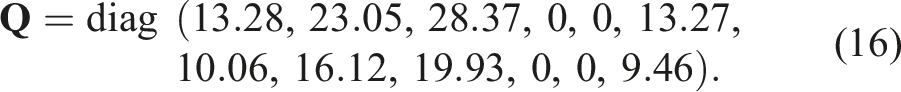
The LQR controller is designed from a linearised state-space representation of the BlueROV2 Heavy dynamics. The complete nonlinear model follows the standard marine vehicle formulation described in Fossen (2011). The state-space matrices A and B used in the LQR design are obtained by linearising this model around an operating point corresponding to a constant reference trajectory. As described in the next section, this trajectory consists of straight-line motion along the x-axis.

The state weighting matrix Q, which penalises the state variables, was determined using the PSO method. This choice was motivated by the ability of PSO to efficiently explore high-dimensional spaces. In an LQR controller, the matrix Q is not required to be diagonal, but it is chosen as such for simplicity and clearer interpretation of penalties for state variables, as it indicates independent penalties (Benner, 2006). For simplification, we do not control the roll and pitch of the drone, as it has been mechanically configured to stabilise around its equilibrium in these directions due to its inertia. Additionally, these axes are minimally affected by the faults considered in the application case scenario detailed in the next section. Therefore, the coefficients of Q associated with roll and pitch are set to zero. The obtained Q matrix is the following:

\begin{align} Q = d i a g & (13.28, 23.05, 28.37, 0, 0, 13.27, \\ 10.06, 16.12, 19.93, 0, 0, 9.46) . \end{align}

(16)

Regarding the control weighting matrix R, given that there is no reason to prioritise the use of one actuator over another, R is designated as the identity matrix I₈. This decision guarantees that all actuators are treated equally and contribute equally to the cost function. The choice of positive definite matrices Q and R ensures that the LQR controller provides a locally stabilising feedback law for the linearised system.

Now that the LQR controller parameters have been defined, the next section focuses on the application case scenario used to evaluate our proposed approach on a BlueROV2 Heavy under thruster fault conditions.

4.2. Application case scenario

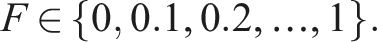
The objective of the chosen scenario is to provide a proof of concept demonstrating the feasibility of integrating DRL-based control reallocation within a linearised model-based control framework, in a simplified yet physically validated experimental configuration. In this work, the application case is restricted to planar motion, where the four horizontal thrusters T₁, T₂, T₃ and T₄ provide an overactuated configuration. The selected scenario, free from additional environmental disturbances, allows isolation of actuator fault effects while preserving overactuation and geometric coupling between surge, sway, and yaw. We consider fault scenarios in which only one actuator is faulty at any time. The single actuator fault is simulated by applying a single fault coefficient F to the input of the faulty thruster, as which takes discrete values of:

F \in {0,0.1, 0.2, \dots, 1} .

The proposed scenario involves following a straight-line trajectory along the x-axis with a fixed desired depth and no desired rotations, with the objective of maintaining control of the AUV despite thruster faults. The reference vector for position and orientation is given by:

w_{ref} = {[\begin{matrix} (x + δ) & 0 & z_{ref} & 0 & 0 & 0 \end{matrix}]}^{T},

(17)

where δ represents an adjustment for trajectory tracking along the x-axis and z_ref is fixed and corresponds to the desired depth of the drone. The velocity components of the reference vector were set to zero.

At the beginning of the mission, the system is at depth z_ref and operates without any fault. At one given position along the x-axis, a fault randomly occurs in one of the four horizontal thrusters. The directions affected by the fault are y and yaw. In simulation, it is assumed that the fault is detected immediately. Upon detection, the DRL-based control reallocation method is activated to manage the fault condition. A threshold for fault detection was determined based on an analysis of the simulation results shown in Section 5, and was applied in real-world conditions. To make the resulting actuator inputs feasible, a truncation is applied on u.

As we are only considering the control of the BlueROV2 Heavy over the x direction and as the objective is to keep the control over each DoF, the CAM must be updated on the line associated with the direction of x. Then, the updated CAM can be reduced to:

W (t) ◦ H = [\begin{matrix} W_{11} (t) H_{11} & \dots & W_{1 r} (t) H_{1 r} \\ H_{21} & \dots & H_{2 r} \\ ⋮ & ⋮ \\ H_{n 1} & \dots & H_{n r} \end{matrix}] .

(18)

The output of the DRL model W(t) can be reduced to the vector:

W (t) = [W_{11} (t), W_{12} (t), W_{13} (t), W_{14} (t)] .

(19)

The DRL continuous action space is defined as [−1,1]⁴, a choice that provides a normalised and symmetric range for learning, which helps stabilise training. Since the agent aims to minimise tracking errors without explicitly controlling the speed, the bounds of the weights help avoid behaviours that are too slow or too fast. In this work, these bounds were chosen by simulating a complete failure of one thruster and manually adjusting the coefficients applied to the remaining thrusters to follow the intended trajectory with minimal deviation and acceptable speed. This process led to the determination that a remapping of the action space to the physical range [0.3,2]⁴ was necessary.

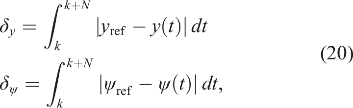
In the fault-free case, BlueROV2 Heavy reaches the target point without deviating from a straight line and with a yaw equal to zero. Thus, the performance evaluation of the hybrid controller in a fault situation is based on the observation of unwanted y error and yaw error. The performance indices for y and yaw are defined as the integral of the error over a given number of time steps, denoted N, where N represents the maximum step (end of an episode), and k corresponds to the step at which the error is detected:

\begin{aligned} δ_{y} = \int_{k}^{k + N} | y_{ref} - y (t) | d t \\ δ_{ψ} = \int_{k}^{k + N} | ψ_{ref} - ψ (t) | d t, \end{aligned}

(20)

where y_ref and ψ_ref are the reference values, both set to zero in our application case.

The objective is to minimise these performance indices, that is, to reduce translational and rotational errors as much as possible. To achieve this objective, the specificities of the DRL model training is described in the next subsection.

4.3. DRL model training on a simulated BlueROV2 Heavy

During the DRL training in simulation, an episode proceeds as follows. As the scenario involves following a straight line along the x-axis, the drone’s position was set to (−1, 0, z_ref) with both linear and angular velocities set to zero. We selected z_ref = −2.5 m, corresponding to the operating depth of the experimental setup. Regarding the reference vector, we experimentally chose δ = 1 m for the straight-line tracking. During the entire episode, the drone was controlled by the LQR controller.

At the beginning of the mission, within the range x = −1.0 m to x = −0.4 m, the system operates without any fault. At x = −0.4 m, a fault occurs in one of the four horizontal thrusters. This position was selected as it affords the actual drone adequate time to stabilise in a straight-line track prior to the onset of a fault. An abnormal behaviour is assumed to be detected instantly and the DRL-based control reallocation is then activated, aiming to manage the fault condition. An appropriate detection threshold for abnormal behaviour was determined based on the results obtained in simulation and then applied to the scenario involving the physical drone, as detailed in Section 5.

The DRL training was conducted on the most severe fault cases, corresponding to thruster efficiencies of 0% and 10%, which could critically jeopardise the success of the AUV mission. Evaluation on less severe faults, with efficiency losses exceeding 10%, was used to evaluate the generalisation capability of the DRL model.

As the aim is to learn to overcome the faults of the four horizontal thrusters individually, at each episode the following happens:

• A thruster T_i, with i ∈ {1, 2, 3, 4}, is randomly selected to experience a fault during the episode;

• An efficiency level is then randomly assigned to thruster T_i, which can either be 0% (representing a total failure) or 10% (representing a partial loss of efficiency).

This process follows the domain randomisation strategy introduced in Section 3, by exposing the agent to varying fault scenarios across episodes. The degrees of freedom impacted by a fault in one of the horizontal thrusters are y and yaw. This is why the reward function r, expressed in Figure 6, aims to minimise the y and yaw errors, which correspond to the following errors of translation (e_T(t)) and rotation (e_R(t)):

e_{T} (t) = | y_{ref} - y (t) |

(21)

e_{R} (t) = | ψ_{ref} - ψ (t) |,

(22)

where y_ref and ψ_ref are both equal to zero. The derivatives of e_T(t) and e_R(t) were added in the expression of the reward, shown as the expression r in Figure 6, to penalise rapid changes in velocity and angular rate, thus avoiding erratic movements. For our application case, the observation vector, which serves as the input to the DRL model, includes the state variables used in the reward function:

y_{obs} (t) = [y (t), \dot{y} (t), ψ (t), \dot{ψ} (t)] .

(23)

Figure 6.

DRL model training scheme (including images from BlueRobotics (2018); Lechene et al. (2024)).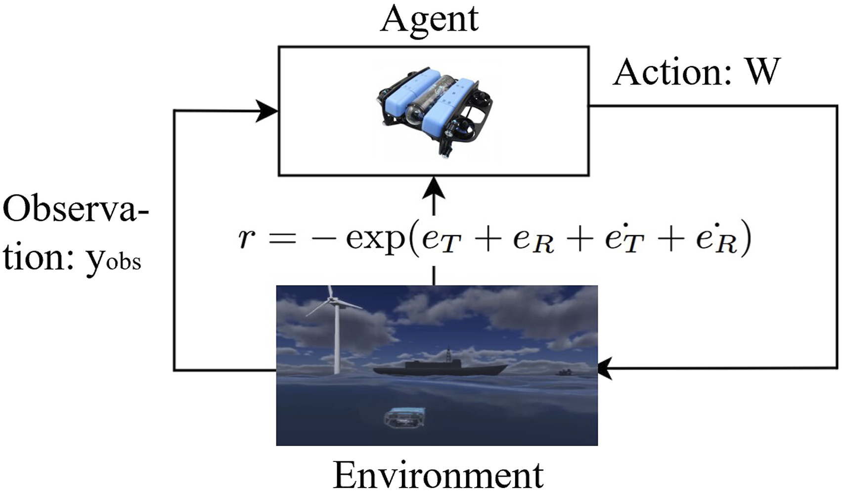

This choice ensures that the agent receives all the necessary information to evaluate the reward and adjust its policy accordingly.

Underwater vehicles exhibit significant inertia due to their mass and drag, which affects their responsiveness to control inputs (Neto et al., 2015). This is why the inertia of the AUV is taken into account in the control reallocation process via a measurement window of size t_w. For each action at time t, the environment produces a feedback at time t + t_w. This gives the DRL model longer-term feedback on the action taken, which increases the efficiency of the training. The CAM is updated with each action taken, that is, each timestep t_w. As no action is taken before receiving the reward from the environment, this is a simplified form of delayed feedback (Howson et al., 2023). This longer-term feedback strategy encourages the agent to learn an action policy that better matches the real dynamics of underwater drones. Combined with domain randomisation during training, which exposes the agent to a variety of fault scenarios, it helps the DRL model transfer to the physical BlueROV2 Heavy. One timestep t_w lasts 0.04 s and an episode ends at step_max = 350 (14 s), as this is the time needed by the hybrid controller to stabilise the behaviour of the drone subject to a fault.

Among the existing DRL algorithms, we chose to use the SAC algorithm (Haarnoja et al., 2018b) because it is sample efficient and leverages entropy maximisation to improve exploration and performance in complex environments with varying disturbances (Haarnoja et al., 2018b). Moreover, since the transition function of the system is unknown, a model-free DRL approach is adopted, allowing the agent to learn an optimal policy directly from interactions with the environment. It has also been demonstrated in the work of Clement et al. (2021) that the SAC algorithm is effective for the control of an AUV.

The SAC algorithm employs an actor-critic architecture, using one actor network to approximate the policy and two critic networks to estimate the state-action value functions, denoted as Q(s_t, a_t). The state-action value function extends the concept of the value function V(s_t) by assessing the expected return of taking a specific action a_t in a given state s_t and then following the policy π_θ(a_t|s_t). Each critic maintains a target network for stable training through soft updates. The SAC algorithm adopts a stochastic policy approach and incorporates principles of maximum entropy reinforcement learning, where an additional term, the entropy temperature, controls the trade-off between reward maximisation and policy entropy. In this work, the implementation of SAC follows the version introduced in Haarnoja et al. (2018a), which employs automatic adjustment of the entropy temperature.

Although potentially noisier, the stochastic nature of the policy improves robustness and exploration (Haarnoja et al., 2018b), which are desirable properties in the context of actuator fault recovery. The actor network is trained to maximise the following objective function:

J (θ) = E_{s_{t} \sim D, a_{t} \sim π_{θ}} [α \log (π_{θ} (a_{t} | s_{t})) - Q_{ϕ} (s_{t}, a_{t})],

(24)

where θ and ϕ are the parameters of the actor and critic networks, respectively, D is the replay buffer, and α is the temperature parameter that controls the trade-off between exploration and exploitation. The critic networks are trained to minimise the following loss function:

\begin{aligned} J_{Q} (ϕ) = E_{(s_{t}, a_{t}, r_{t}, s_{t + 1}) \sim D} [(Q_{ϕ} (s_{t}, a_{t}) - (r_{t} \\ {+ γ E_{a_{t + 1} \sim π_{θ}} [Q_{\bar{ϕ}} (s_{t + 1}, a_{t + 1}) - α \log (π_{θ} (a_{t + 1} | s_{t + 1}))]))}^{2}] . \end{aligned}

(25)

where

\bar{ϕ}

denotes the parameter of the target critic network and r_t is the immediate reward.

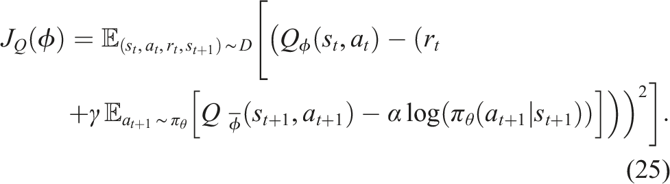
The pseudocode of the SAC algorithm is presented in Algorithm 1.

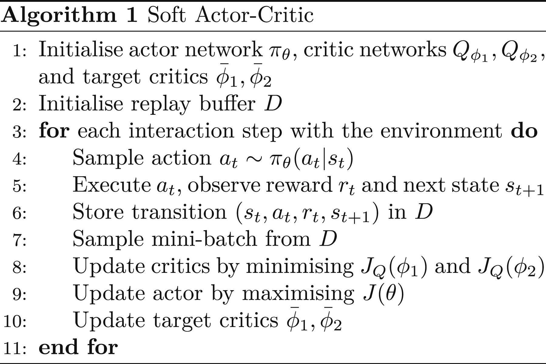
The main advantages of SAC are its sample efficiency, its ability to handle continuous action spaces, and its stochastic policy, which improves robustness to uncertainties. On the other hand, the method relies on multiple neural networks, which can increase computational demand (Haarnoja et al., 2018b). These characteristics explain the choice of SAC for our application, where adaptability to actuator faults is essential.

During training, the choice of DRL hyperparameters (e.g., learning rate, discount factor) strongly influences the behaviour of W(t): high learning rates may cause oscillatory or unstable updates, whereas too small values slow convergence. These hyperparameters also affect the robustness of the policy and its ability to generalise from simulation to real-world conditions. The selected hyperparameters for the SAC algorithm follow the standard configuration commonly adopted in the literature (Haarnoja et al., 2018b). These default settings have been validated through extensive research and facilitate reproducibility. The hyperparameters that are used in our application case are shown in Table 1.

Table 1.

Chosen hyperparameters for the SAC algorithm.

Hyperparameter	Value
Learning rate (Actor: θ, Critic: ϕ)	3 × 10⁻⁴
Discount factor (γ)	0.99
Target network update rate	0.005
Replay buffer (D) size	1 × 10⁶
Batch size	256
Number of hidden units	256
Number of hidden layers	2
Activation function	ReLU

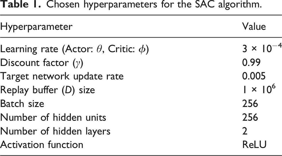
In our implementation, the learning rate was kept constant, as is standard practice in SAC, since the Adam optimiser already provides adaptive step-size adjustment. Moreover, automatic entropy tuning in SAC removes the need to manually specify a reward scale.

Regularisation is essential to smooth the outputs and avoid infeasible changes in W(t). For this purpose, a moving average low-pass filter is added to the output of the DRL model in order to attenuate variations in the CAM, with the objective of approaching global stability, as discussed in Section 3. This type of filter is chosen for its ease of tuning, as it only requires the selection of a fixed window size and does not involve parameter coupling. However, other post-processing techniques capable of limiting abrupt variations could be employed depending on the application requirements. The transfer function of the selected moving average filter is given by:

H (z) = \frac{1}{N_{W}} \sum_{n = 0}^{N_{W} - 1} z^{- n},

(26)

where N_W denotes the window size of the moving average and z⁻ⁿ represents a time shift. Low-pass filters introduce a phase delay, which can degrade closed-loop stability if not properly tuned (Franklin et al., 2002). To mitigate this issue, N_W must be carefully selected: it should be high enough to preserve the responsiveness of the control actions, while still sufficiently low to attenuate abrupt variations. Through experimental tuning, N_W was set to 15 in order to achieve a suitable compromise between smoothing the output of the DRL model and maintaining sufficient responsiveness to changes in the system. To assess the performance of the proposed hybrid controller, hereafter denoted as the LQR-SAC controller, tests were conducted across various fault scenarios and the LQR-SAC controller was compared with a standard LQR controller and a conventional adaptive LQR controller, as detailed in the next section.

5. Results

This section presents the process of evaluation and shows the obtained results, both in simulation and on a physical BlueROV2 Heavy.

5.1. Performance evaluation methodology

The evaluation scenario involves tracking along the x-axis, starting from the initial point (−1, 0, −2.5), with a thruster fault introduced at x = −0.4 m. The controller’s recovery performance is evaluated using the performance indices δ_y and δ_yaw detailed in equation (20).

For the evaluation of recovery performance in simulation, we consider all the possible thruster faults individually: the considered faults include 11 levels of efficiency loss for each thruster: F ∈ {0, 0.1, 0.2, …, 1}. This approach includes scenarios encountered during training, F ∈ {0, 0.1}, as well as similar but unseen scenarios, with F ∈ {0.2, …, 1}. This enables an evaluation of the LQR-SAC controller’s generalisation capability, as it allows us to observe how effectively the controller performs in new conditions beyond those specifically used in training.

To assess the performance of the proposed LQR-SAC controller, we will not only evaluate it across various fault scenarios but also compare it with a standard LQR controller and a conventional adaptive LQR controller. The standard LQR controller involves applying the LQR controller on the faulty AUV without the use of DRL and without any control reallocation. The standard LQR controller was included only as a baseline reference to illustrate the limitations of a non-adaptive strategy under actuator faults.

To provide a fair comparison with the proposed LQR-SAC controller, which is a type of adaptive controller, we include another adaptive LQR method designed to overcome actuator faults. This other adaptive LQR controller relies on the same weighting matrices as those used by the LQR-SAC controller, in particular the same Q matrix optimised with the PSO method. This is a direct adaptive method which does not use DRL but instead involves updating the controller gains by applying the MIT rule (Mareels et al., 1987) to the LQR weighting matrices. The purpose of this approach is to react quickly to actuator faults by increasing the weights associated with the errors between the desired and observed movements. In our case, the impacted degrees of freedom are y and yaw. For the LQR controller that we consider, the direct adaptive method will involve updating the values in the state weighting matrix Q associated with the y and yaw directions, respectively, denoted Q_y and Q_ψ, using the MIT rule:

Q_{y} = Q_{y} + α_{y} \cdot e_{T}^{2}

(27)

Q_{ψ} = Q_{ψ} + α_{ψ} \cdot e_{R}^{2},

(28)

where α_y and α_ψ are the adaptation gains that modulate the impact of the error on the adjustment of Q. The higher the error in these directions, the greater the increase in the corresponding values in the matrix Q defined in equation (14), which in turn increases their weight in the cost function described in equation (14). Regarding the tuning parameters of the MIT rule, they were determined by iteratively adjusting the tuning parameters to minimise the deviations without inducing oscillations in the system, in the worst fault case scenario that we consider, that is, where one of the thrusters is at 0% efficiency. The obtained tuning parameters are α_y = 0.8 for the y error and α_θ = 0.02 for the yaw error. This direct adaptive LQR controller was selected because it does not rely on explicit fault diagnosis, ensuring a consistent comparison with the proposed diagnosis-free reallocation strategy.

Next section shows the obtained results in simulation.

5.2. Simulation results

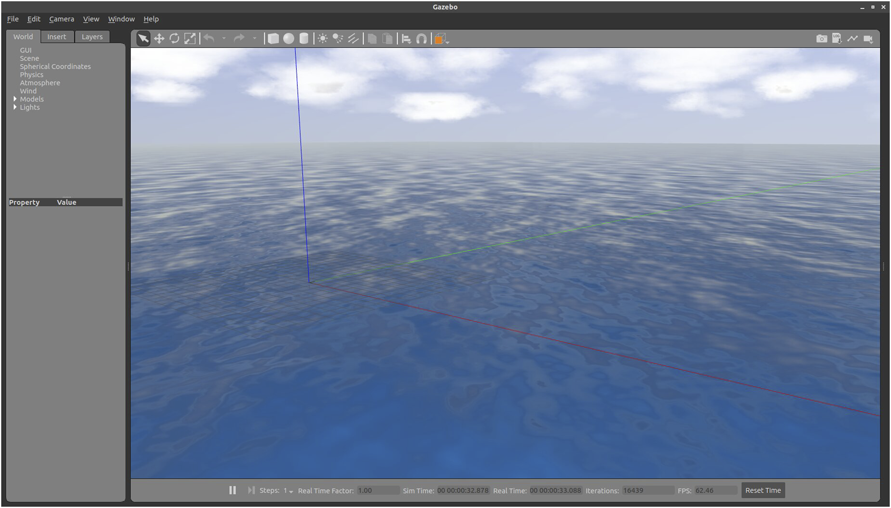
The chosen simulation software is GAZEBO Simulator (Koenig and Howard, 2004) and the plugin employed to model the underwater environment is UUV Simulator (Manhães et al., 2016). Figures 7 and 8 show the BlueROV2 Heavy model and the marine environment in GAZEBO with the UUV Simulator plugin.

Figure 7.

BlueROV2 Heavy model with UUV Simulator (Manhães et al., 2016).

Figure 8.

Illustration of the marine environment with UUV Simulator (Manhães et al., 2016).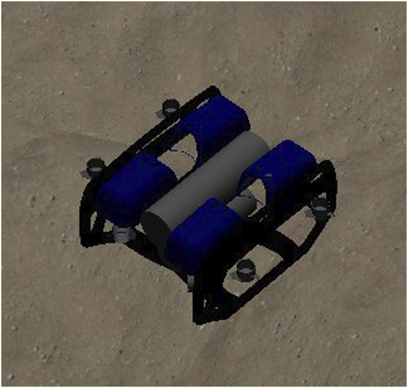

In this work, the robot operating system (ROS) (Quigley et al., 2009) framework was used for sensor communication and actuator control. ROS provides communication bridges to enable the transmission of data inside the GAZEBO simulations. To train the DRL agent, we selected the SAC algorithm from the Stable-Baselines3 library (Raffin et al., 2021), as it offers a well-documented and efficient implementation of state-of-the-art DRL algorithms. The integration between Stable-Baselines3 and ROS, which enables interaction between the learning agent and the simulated environment, is detailed in Lagattu et al. (2025b). The training of the DRL model was carried out in simulation as detailed in Section 4. The full training lasted for 100,000 steps and took approximately 7 hours on a laptop with 32 GB of RAM, using one CPU core without parallelisation and no GPU acceleration.

The mean reward curve of this training is displayed in Figure 9. This figure illustrates the progression of the DRL model’s mean reward over training as a function of the number of training steps. It can be observed that a minimum of 40, 000 steps was required to achieve convergence.

Figure 9.

Mean episode reward of the DRL model over number of steps.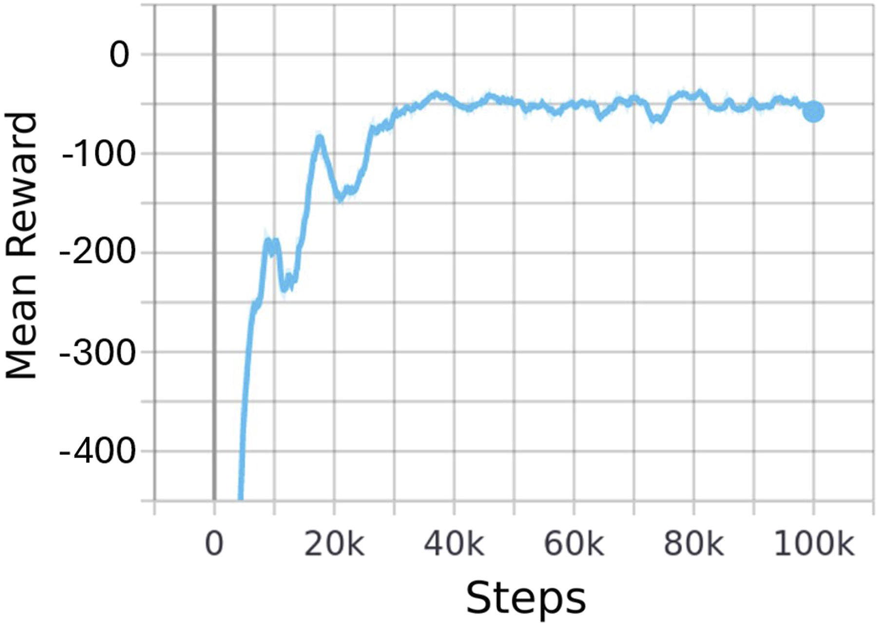

Evaluation of the trained DRL model is performed on the standard LQR, conventional adaptive LQR, and LQR-SAC controllers, considering thrusters subject to severe faults (0% and 10% efficiency) encountered during training, as well as less severe faults (above 10% efficiency) that were not seen during training. Table 2 reports the mean and standard deviation of the y and yaw performance indices, computed over 100 episodes for each horizontal thruster (T₁ to T₄) and each efficiency level (from 0% to 100%), and then averaged across all four thrusters.

Table 2.

Mean and standard deviation of performance indices for the 4 thrusters evaluated individually from 0% (total failure) to 100% efficiency with standard LQR, conventional adaptive LQR and LQR-SAC controllers, evaluated over 100 episodes in simulation for each case.

	0%		10%		20%		30%		40%		50%		60%		70%		80%		90%		100%
	δ _y	δ _yaw	δ _y	δ _yaw	δ _y	δ _yaw	δ _y	δ _yaw	δ _y	δ _yaw	δ _y	δ _yaw	δ _y	δ _yaw	δ _y	δ _yaw	δ _y	δ _yaw	δ _y	δ _yaw	δ _y	δ _yaw
Standard LQR	33.58 ± 0.09	39.42 ± 0.12	30.68 ± 0.05	36.12 ± 0.10	28.54 ± 0.05	33.76 ± 0.09	26.24 ± 0.06	29.82 ± 0.08	25.06 ± 0.04	27.87 ± 0.07	19.33 ± 0.03	23.08 ± 0.06	14.54 ± 0.02	20.80 ± 0.04	11.60 ± 0.03	17.50 ± 0.04	7.37 ± 0.02	10.62 ± 0.02	4.19 ± 0.01	6.25 ± 0.01	0.00 ± 0.00	0.00 ± 0.00
Adaptive LQR	28.56 ± 0.13	30.17 ± 0.31	26.34 ± 0.15	28.10 ± 0.26	23.61 ± 0.11	26.09 ± 0.25	20.09 ± 0.09	22.51 ± 0.19	18.86 ± 0.06	21.24 ± 0.15	16.83 ± 0.02	17.21 ± 0.16	12.93 ± 0.03	14.27 ± 0.11	10.11 ± 0.02	11.90 ± 0.08	7.21 ± 0.02	8.50 ± 0.08	3.51 ± 0.02	5.06 ± 0.05	0.00 ± 0.00	0.00 ± 0.00
LQR-SAC	8.77 ± 0.06	16.77 ± 0.14	7.61 ± 0.05	15.10 ± 0.13	7.02 ± 0.03	13.92 ± 0.10	6.88 ± 0.03	13.08 ± 0.11	5.78 ± 0.01	12.11 ± 0.08	5.37 ± 0.01	11.56 ± 0.05	5.04 ± 0.01	11.04 ± 0.02	4.85 ± 0.01	10.54 ± 0.01	2.69 ± 0.01	9.19 ± 0.01	2.31 ± 0.01	6.46 ± 0.01	0.83 ± 0.00	3.17 ± 0.01

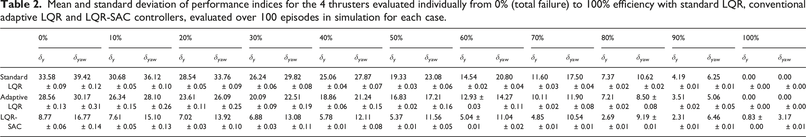
At 0% thruster efficiency, the LQR-SAC controller reduced the y error by approximately 73.9% and 69.3% compared to the standard LQR and the adaptive LQR controllers, respectively. In terms of yaw error, reductions of 57.5% and 44.4% were achieved. Similarly, at 10% efficiency, the LQR-SAC controller achieved reductions of 75.2% and 71.1% in y error, and 58.2% and 46.3% in yaw error compared to the same benchmarks.

The superior performance of the LQR-SAC controller suggests that the DRL agent effectively learned to handle these efficiency levels during training. The lower performance of the conventional adaptive LQR can be attributed to its lack of consideration for the thruster geometric configuration, as it only adjusts the relative importance of the state error. As a result, this method quickly drives the thrusters to saturation since the forces are not properly redistributed. The LQR-SAC controller also outperformed other controllers at 20% to 70% efficiency levels which were not applied during training, showing the generalisation capability of the DRL model. Beyond 70% efficiency, conventional adaptive LQR control outperforms LQR-SAC control in reducing the yaw error, as increased gains suffice at low fault levels. Beyond 90% efficiency, the LQR-SAC control underperforms due to limited generalisation when facing scenarios that diverge significantly from those encountered during training. These results suggest a fault detection threshold, experimentally determined at y = ±0.1 m, beyond which the LQR-SAC controller is preferable to the standard LQR or the conventional adaptive LQR controller. To assess whether the differences observed between two sets of results are statistically significant, the Z-test for difference of means (Montgomery and Runger, 2010) is employed. This test computes a p-value, which quantifies the likelihood of observing such differences under the null hypothesis of equal means. If the p-value is below a predefined significance level, commonly α = 0.05, the null hypothesis is rejected.

This test is applied to the results presented in Table 2, to provide a comparison, on the one hand, between the LQR-SAC controller and the standard LQR controller, and on the other hand, between the LQR-SAC controller and the adaptive controller. All computed p-values are lower than 10⁻¹⁵, highlighting the high statistical significance of the results. The LQR-SAC controller’s superior performance can be attributed to the DRL-based method’s effective control reallocation policy learned during training, eliminating the need for explicit fault diagnosis. However, there is room for improvement, as it is theoretically possible to achieve zero error in y and yaw, given that the system remains sufficiently actuated to maintain control over the forces applied on each DoF. The next section details the results obtained on the physical BlueROV2 Heavy, using the same DRL model trained in simulation.

5.3. Results on physical BlueROV2 Heavy

To validate the proposed approach under real-world conditions, experiments were conducted using a BlueROV2 Heavy in the 6 m × 6 m × 3 m immersion tank at Flinders University. The localisation of the drone was determined using an ArUco marker tracker (Garrido-Jurado et al., 2014) and a depth sensor. The ArUco marker was tracked by a camera positioned slightly below the surface as shown in Figure 10, and its data were merged with a Kalman filter incorporating measurements from the inertial measurement unit (IMU) and the depth sensor.

Figure 10.

BlueROV2 Heavy in the test pool, with the localisation system.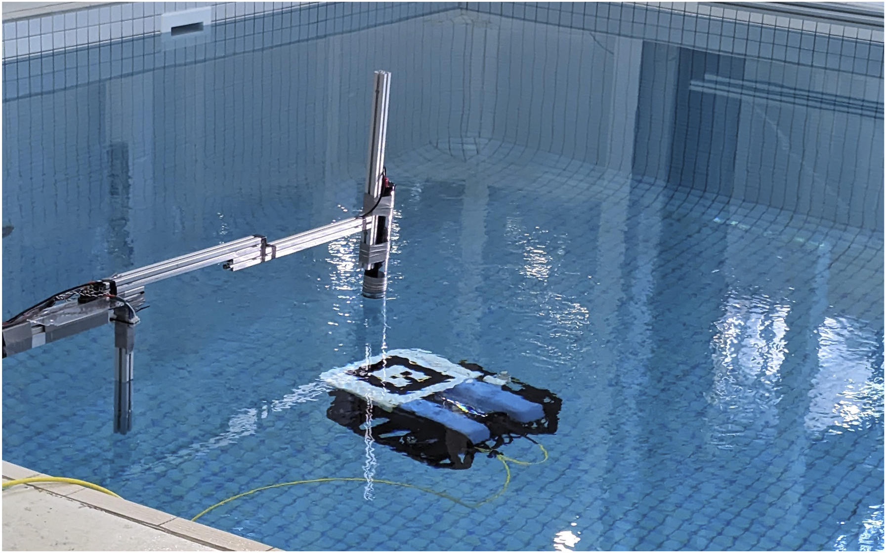

The detailed positioning system of the experiments is provided in Chaffre et al. (2025), where the same configuration was employed for the real-world tests. The sensor data were transmitted via a tether to a laptop with 32 GB of RAM, where the controller outputs were also calculated. Each episode consists of a scenario instance involving the tracking of a straight line and the occurrence of a thruster fault, as described in Section 5. The DRL model is used when an abnormal behaviour is detected. The sensor data and control inputs are saved in a rosbag (Quigley et al., 2009) for each episode. A rosbag is a file format used to record and store data exchanged between different nodes in a ROS-based system. The inference time of the DRL agent, measured over all inference steps during the real-world experiments (10 evaluation episodes per fault case), averaged 0.048 s, matching the sensor data reception frequency and confirming real-time feasibility.

The proposed LQR-SAC controller outputs directly the thruster inputs, yet the onboard system of the BlueROV2 Heavy is not designed to handle direct thruster control, necessitating the use of a conversion step. As it was not possible to send thruster inputs directly to the drone, the CAM was applied at the end of the process to convert thruster inputs into forces. Although this resulted in a loss of information, the behaviour of the drone remained similar to that observed in simulation. To assess the number of episodes required for an accurate estimation of the results, we used the proposed LQR-SAC control approach over 20 episodes. During this, the mean y error, which serves as a performance measure, along with the standard deviation, were recorded over an increasing number of episodes up to 20. The results can be seen in Figure 11, where we can see that the performance converges after 10 episodes. Therefore, we chose to evaluate each fault case over 10 episodes on the real robot, with each set of 10 episodes taking approximately 30 minutes.

Figure 11.

Mean of y error, with standard deviation across the number of episodes (or rosbags) considered.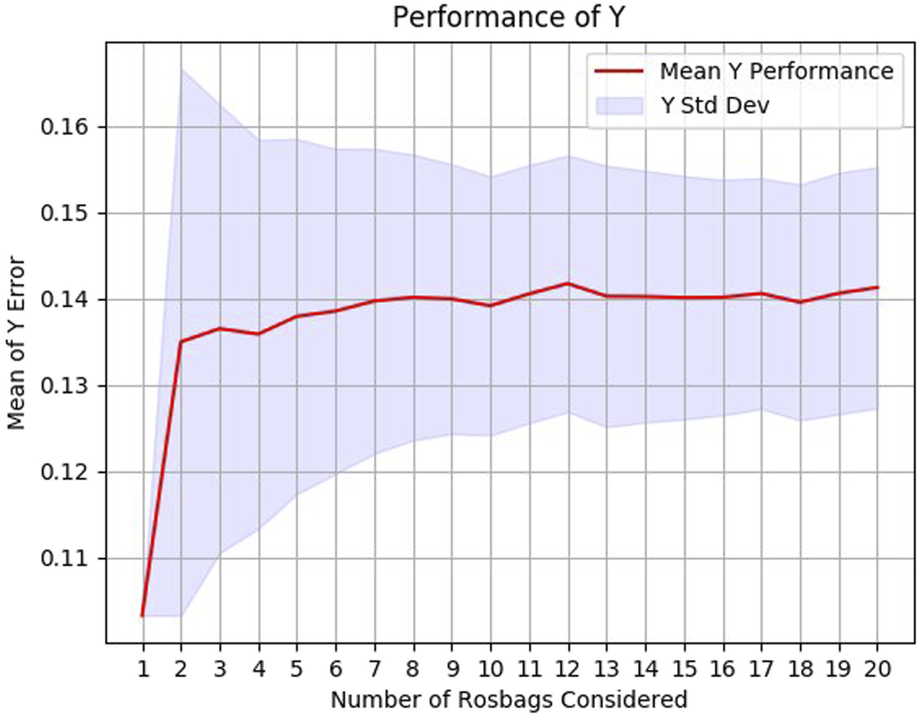

To reduce the time required for experiments, specific levels of thruster efficiency were selected for testing on the physical BlueROV2 Heavy: 0%, 10%, 40%, and 70%, corresponding to f ∈ {0, 0.1, 0.4, 0.7}. This selection allows for the evaluation of the most severe faults encountered during training in simulation, and of less severe faults that were not encountered during training, while staying within the range where the DRL model can still be efficient. This evaluation was performed on each horizontal thruster individually and the results are displayed in Table 3.

Table 3.

Mean and standard deviation of performance indices for the 4 thrusters evaluated individually, with 0%, 10%, 40%, and 70% efficiency with standard LQR, conventional adaptive LQR and LQR-SAC controllers, evaluated over 10 episodes on a physical BlueROV2 Heavy for each case.

	0%		10%		40%		70%
	δ _y	δ _yaw	δ _y	δ _yaw	δ _y	δ _yaw	δ _y	δ _yaw
Standard LQR	25.30 ± 2.35	39.78 ± 4.21	22.37 ± 2.47	28.13 ± 2.82	16.20 ± 1.38	24.38 ± 6.09	10.79 ± 1.16	22.47 ± 5.44
Adaptive LQR	16.49 ± 3.09	65.30 ± 6.62	14.53 ± 0.66	49.30 ± 5.25	12.64 ± 1.91	21.07 ± 3.15	5.07 ± 1.00	17.65 ± 2.00
LQR-SAC	11.95 ± 1.09	28.32 ± 1.89	8.40 ± 1.13	23.69 ± 4.87	5.96 ± 0.17	17.56 ± 3.60	3.87 ± 0.35	13.95 ± 2.34

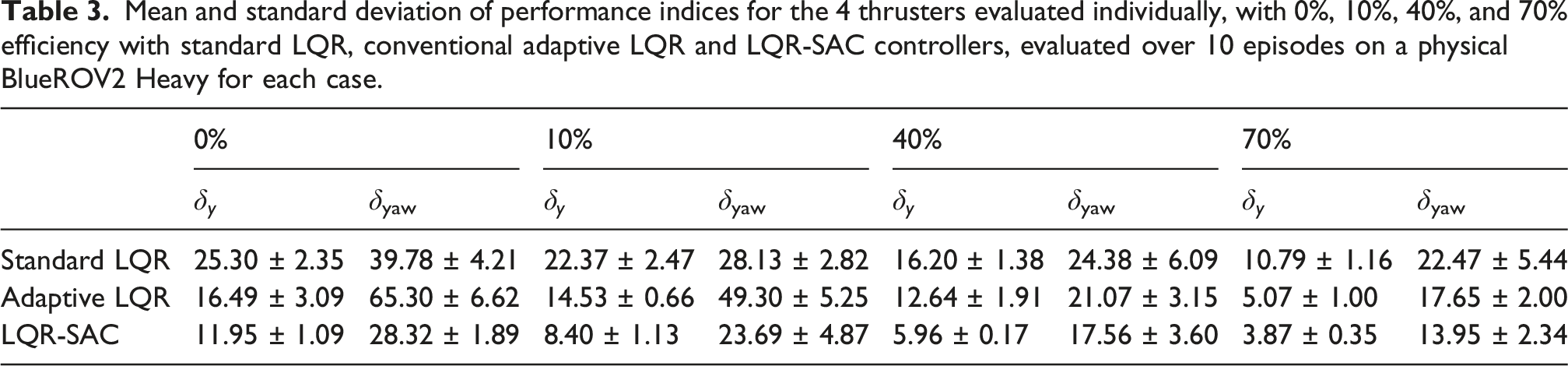
At 0% thruster efficiency, the LQR-SAC controller achieved approximately 52.4% and 28.6% reductions in y error compared to the standard LQR and the conventional adaptive LQR controllers, respectively. In terms of yaw error, reductions of 16.7% and 56.5% were observed. Similarly, at 10% efficiency, it improved y error by 62.45% and 41.2%, and yaw error by 16.7% and 52.4% relative to the same benchmarks. Unlike in simulation, the standard LQR controller outperforms the conventional adaptive controller at both 0% and 10% efficiency. The discrepancies between simulation and real-world results may be due to the approximation of the drone model in simulation and to the presence of a cable attached to the drone, which may cause drifting. At 40% and 70% efficiency, the LQR-SAC controller outperforms the compared controller, as observed in simulation.

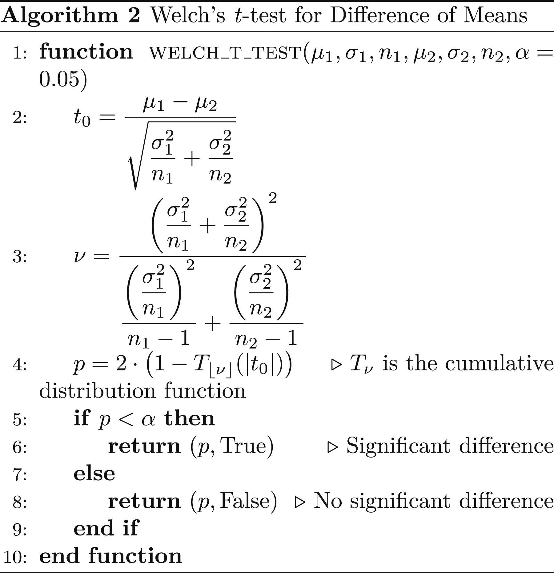
To assess whether the observed performance differences between controllers on the physical AUV are statistically significant, Welch’s t-test, a variation of Student’s t-test, is employed (Montgomery and Runger, 2010). It evaluates whether the means of the two samples differ significantly without assuming homogeneity of variance. In this study, the normal probability plot was examined, indicating that there is no issue with the normality assumption, which supports the use of Welch’s test. From this test statistic, described in Algorithm 2, a p-value is obtained. In this context, μ₁ and μ₂ represent the means of the two independent samples, while σ₁ and σ₂ denote their respective standard deviations. Additionally, n₁ and n₂ represent the sizes of the two independent samples being compared.

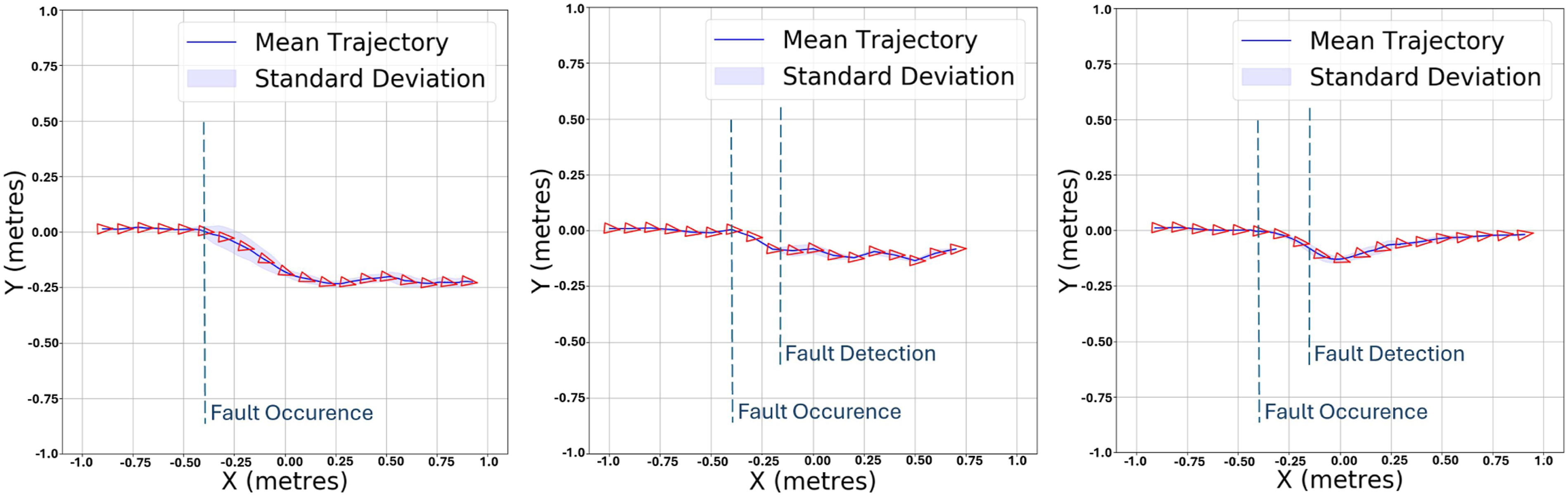
Tables 4 and 5 present the obtained p-values. As in the simulation results, the p-values are extremely small, indicating the statistical significance of the performance differences between LQR-SAC controller and the compared controllers.

Table 4.

P-value computation for y error across efficiency levels from 0% to 70%, using physical drone data.

	LQR-SAC/Standard	LQR-SAC/Adaptive LQR
0%	4.80e-13	6.03e-06
10%	1.89e-13	1.28e-10
40%	3.14e-11	4.39e-08
70%	1.63e-10	5.63e-4

Table 5.

P-value computation for yaw error across efficiency levels from 0% to 70%, using physical drone data.

	LQR-SAC/Standard	LQR-SAC/Adaptive LQR
0%	7.60e-10	1.64e-13
10%	1.15e-4	5.77e-15
40%	1.21e-05	1.81e-04
70%	1.63e-06	1.24e-08

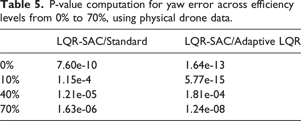
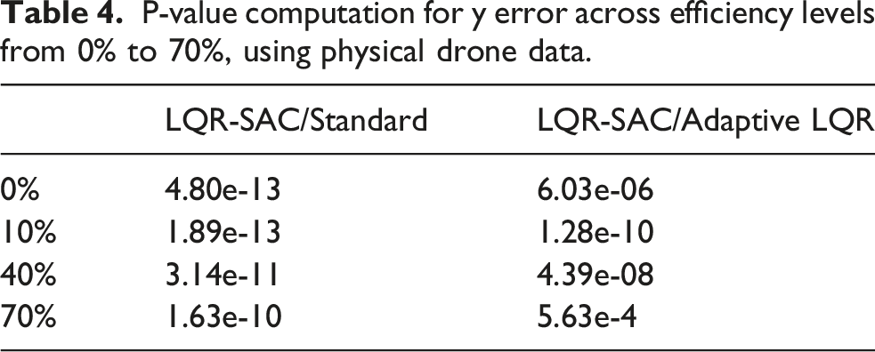
To better visualise the results, Figures 12 –15 illustrate the mean and standard deviation of the 2D trajectory of the BlueROV2 Heavy, controlled by three different controllers: the standard LQR (left), conventional adaptive LQR (middle), and LQR-SAC (right) controllers. Each set of images shows the trajectory of the AUV using these controllers, under two different thruster efficiencies. Figure 12 displays the results at 0% efficiency of T₁, with each controller tested over 10 evaluation runs. Figure 13 then presents the results at 40% efficiency of T₁. Similarly, Figure 14 shows the trajectories at 0% efficiency of T₂, and finally, Figure 15 illustrates the outcomes at 40% efficiency of T₂. From these figures, we observe that in the case of the standard LQR, there is a significant deviation from the straight-line path, with BlueROV2 Heavy deviates entirely, either towards negative y values for T₁ or positive y values for T₂. Regarding the conventional adaptive LQR, an improvement over the standard LQR can be seen, as the trajectory of BlueROV2 Heavy appears to self-correct slightly and deviate less than with the standard LQR controller.

Figure 12.

Mean and standard deviation of the 2D trajectory of the BlueROV2 Heavy controlled by the standard LQR (left), conventional adaptive LQR (middle) and LQR-SAC (right) controllers at 0% efficiency of T₁, over 10 evaluation tests.

Figure 13.

Figure 14.

Figure 15.

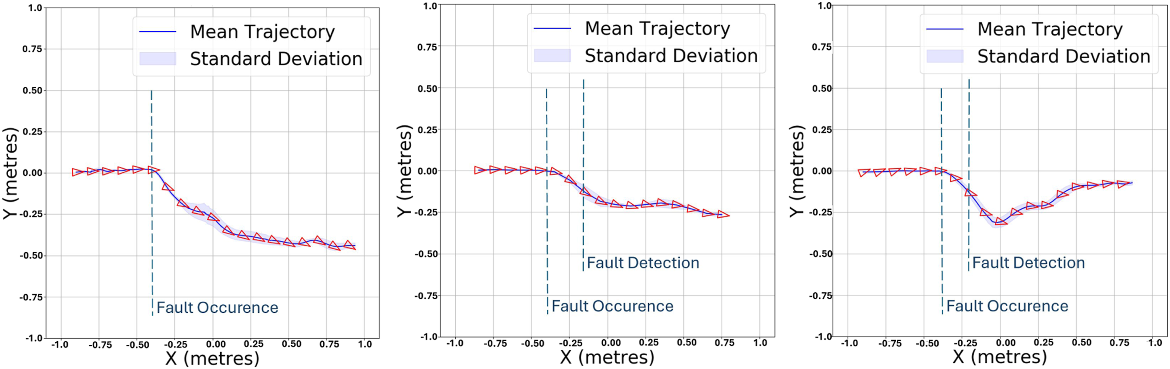
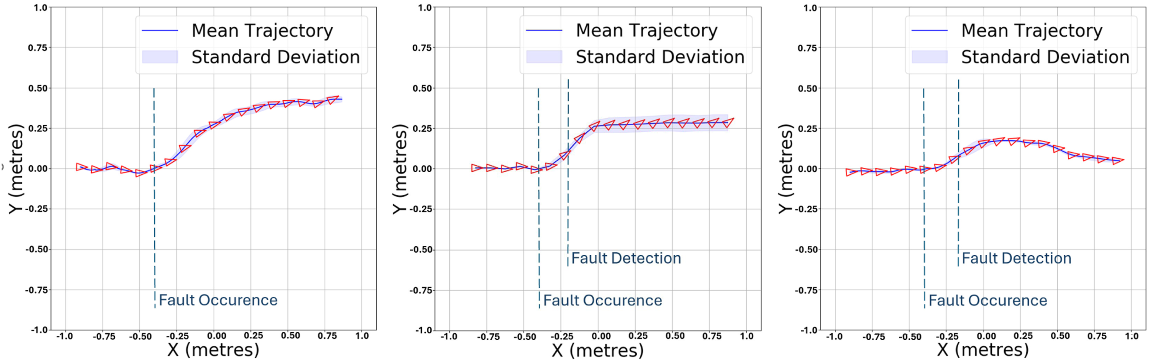
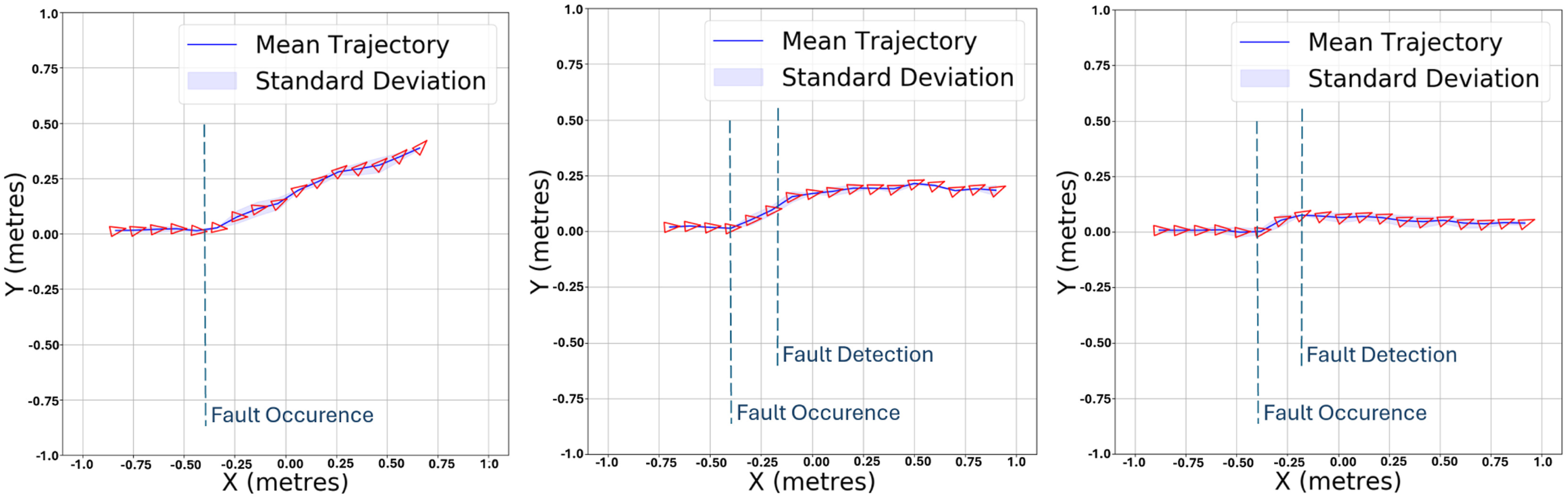
We can see that the LQR-SAC controller significantly outperforms both the standard LQR and the conventional adaptive LQR for the y error, as the drone’s trajectory, after the fault is detected, aligns more closely with the straight line.

These observations suggest that direct adaptation of the LQR helps limit deviation by increasing the value of the Q matrix associated with y-axis errors, which increases the importance of correcting these deviations in the LQR cost function. However, this is insufficient; notably in Figure 14, we observe a yaw orientation error that grows significantly. This is due to the fact that as in simulation, the direct adaptive approach does not redistribute forces among the actuators and does not account for the geometric configuration of the BlueROV2 Heavy’s thrusters.

The observed performance of the LQR-SAC controller indicates that the CAM update by DRL allows for an overall better trajectory correction, as it enables a redistribution of forces. It suggests that the DRL model implicitly recognises the faults, relying on knowledge from training to identify the faulty behaviour of the BlueROV2 Heavy and learn how to redistribute forces among the actuators correctly despite the fault.

6. Conclusion

Actuator faults in dynamic systems can lead to performance degradation or mission failure due to the inability of traditional control systems to adapt to faults without explicit diagnosis. This paper presented a new method allowing control reallocation to recover from actuator faults in autonomous dynamic systems without any explicit fault diagnosis, using a DRL method in a model-based control framework. The goal of this approach is to rely on the adaptability of DRL to overcome actuator faults, while keeping a robust control framework. This approach was tested both in simulation and on a physical BlueROV2 Heavy by inserting thruster faults during waypoint navigation along the x-axis. The LQR controller was selected for this application case, and incorporating the CAM into the gain computation allowed local stability in the presence of actuator faults.

The proposed controller was compared to a standard LQR controller and to a conventional adaptive LQR controller. In simulation, the LQR-SAC controller showed an improvement compared to a standard LQR controller and a conventional adaptive LQR controller under 70% efficiency. The effectiveness of the trained model was demonstrated on faults not encountered during training, highlighting the generalisability of the LQR-SAC controller.

On the physical drone, the LQR-SAC controller also demonstrated an improvement compared to the other controllers. However, some differences were observed between the experimental results and those obtained in simulation, which could be attributed to an inaccurate modelling of the drone in the simulation environment. A potential way to address this issue would be to train the DRL model in simulation with environments featuring varying parameters.

The experimental validation was restricted to a simplified surge-direction trajectory in order to provide a clear proof of concept and to demonstrate the feasibility of transferring a DRL-trained policy from simulation to the physical AUV. While this setup does not address broader challenges such as scalability, nonlinear behaviours, or complex trajectories, future work will extend the validation to multi-DoF missions, more complex actuator faults, and environmental disturbances. In this work, ocean currents were neglected to isolate actuator fault effects and clearly assess the proposed controller. A constant current acts as a persistent disturbance in the vehicle dynamics and must be handled at the model-based control level through appropriate compensation or estimation mechanisms. Future work will address this extension explicitly.

A promising future direction is the exploration of hybrid strategies combining model-based control with self-supervised learning (Ericsson et al., 2022). Such approaches could enable the system to autonomously adapt to fault-related patterns without requiring explicit diagnosis, further enhancing fault tolerance. Another perspective is to address the challenge of state estimation uncertainty by introducing sensor noise during the DRL training phase and by relying on proper sensor fusion on the physical platform rather than on an external camera-based tracking system. This would enable the controller to be evaluated under more realistic conditions, where state estimation uncertainties are explicitly taken into account.

Footnotes

Acknowledgement

The authors would like to thank Andrew Lammas and Jonathan Wheare from Flinders University for their assistance with the experiments. Their support and expertise greatly contributed to the success of this work.

ORCID iDs

Katell Lagattu

Thomas Chaffre

Karl Sammut

Ethical considerations

There are no human participants in this article and informed consent is not required.

Author Contributions

Katell Lagattu: Conceptualisation, methodology, formal analysis, investigation and writing – original draft preparation. Ramy Alham: Methodology and writing – original draft preparation. Thomas Chaffre: Investigation and writing – review and editing. Eva Artusi, Paulo E. Santos, and Benoit Clement: Conceptualisation, methodology and writing – review and editing. Gilles Le Chenadec: Conceptualisation, formal analysis and writing – review and editing. Karl Sammut: Conceptualisation, investigation and writing – review and editing.

Funding

The authors disclosed receipt of the following financial support for the research, authorship, and/or publication of this article: The authors disclosed receipt of the following financial support for the research, authorship, and/or publication of this article: This work was supported by the French Defence Innovation Agency (AID), Naval Group, Flinders University and ENSTA.

Declaration of conflicting interests

The authors declared no potential conflicts of interest with respect to the research, authorship, and/or publication of this article.

References

Abbaspour

Mokhtari

Sargolzaei

, et al. (2020) A survey on active fault-tolerant control systems. Electronics 9(9): 1513. https://doi.org/10.3390/electronics9091513

Ahmadzadeh

Kormushev

Caldwell

(2014) Multi-objective reinforcement learning for AUV thruster failure recovery. In: 2014 IEEE Symposium on Adaptive Dynamic Programming and Reinforcement Learning (ADPRL). IEEE. ISBN 978-1-4799-4552-8, pp. 1–8.

Amin

Hasan

(2019) A review of fault tolerant control systems: advancements and applications. Measurement 143: 58–68. https://doi.org/10.1016/j.measurement.2019.04.083

Atassi

Khalil

(1999) A separation principle for the stabilization of a class of nonlinear systems. IEEE Transactions on Automatic Control 44(9): 1672–1687. https://doi.org/10.1109/9.788534

Barata

JCA

Hussein

(2012) The Moore–Penrose pseudoinverse: a tutorial review of the theory. Brazilian Journal of Physics 42: 146–165. https://doi.org/10.1007/s13538-011-0052-z

Benner

(2006) Control theory. In: Handbook of Linear Algebra, pp. 1–57.

Benosman

(2011) Passive fault tolerant control. In: Robust Control Theory Appl, pp. 9.

Bhan

Quinones-Grueiro

Biswas

(2021) Fault tolerant control combining reinforcement learning and model-based control. In: 2021 5th International Conference on Control and Fault-Tolerant Systems (SysTol), pp. 31–36.

BlueRobotics (2018) Introducing the bluerov2 heavy. Available at: https://bluerobotics.com/introducing-bluerov2-heavy/ (Accessed 23 January 2025).

10.

Bradtke

(1992) Reinforcement learning applied to linear quadratic regulation. Advances in Neural Information Processing Systems 5: 295–302.

11.

Brosilow

Joseph

(2002) Techniques of Model-based Control. Prentice Hall Professional.

12.

Chaffre

(2023) Reinforcement Learning and Sim-to-Real Transfer for Adaptive Control of AUV. Flinders University. Phd thesis.

13.

Chaffre

Moras

Chan-Hon-Tong

, et al. (2021) Learning-based vs model-free adaptive control of a mav under wind gust. URL. https://arxiv.org/abs/2101.12501

14.

Chaffre

Wheare

Lammas

, et al. (2025) Sim-to-real transfer of adaptive control parameters for auv stabilisation under current disturbance. The International Journal of Robotics Research 44(3): 407–430. https://doi.org/10.1177/02783649241272115

15.

Clement

Chaffre

Le Chenadec

, et al. (2021) Direct adaptive pole-placement controller using deep reinforcement learning: application to auv control. IFAC-PapersOnLine 54(16): 333–340. https://doi.org/10.1016/j.ifacol.2021.10.113

16.

Clerc

Kennedy

(2002) The particle swarm-explosion, stability, and convergence in a multidimensional complex space. IEEE Transactions on Evolutionary Computation 6(1): 58–73. https://doi.org/10.1109/4235.985692

17.

De Kleer

Williams

(1987) Diagnosing multiple faults. Artificial Intelligence 32(1): 97–130. https://doi.org/10.1016/0004-3702(87)90063-4

18.

Dulac-Arnold

Levine

Mankowitz

, et al. (2020) An empirical investigation of the challenges of real-world reinforcement learning. CoRR abs/2003.11881.

19.

Ericsson

Gouk

Loy

, et al. (2022) Self-supervised representation learning: introduction, advances, and challenges. IEEE Signal Processing Magazine 39(3): 42–62. https://doi.org/10.1109/msp.2021.3134634

20.

Ernits

Dearden

Pebody

(2010) Automatic fault detection and execution monitoring for auv missions. In: IEEE/OES Autonomous Underwater Vehicles, pp. 1–10.

21.

Fei

, et al. (2020) Learn-to-recover: retrofitting uavs with reinforcement learning-assisted flight control under cyber-physical attacks. In: 2020 IEEE International Conference on Robotics and Automation (ICRA), pp. 7358–7364.

22.

Fossen

(2011) Handbook of Marine Craft Hydrodynamics and Motion Control. Wiley.

23.

François-Lavet

Henderson

Islam

, et al. (2018) An introduction to deep reinforcement learning. Foundations and Trends® in Machine Learning 11(3-4): 219–354. https://doi.org/10.1561/2200000071

24.

Franklin

Powell

Emami-Naeini

, et al. (2002) Feedback Control of Dynamic Systems, Volume 4. Prentice hall Upper Saddle River.

25.

Gao

Cecati

Ding

(2015) A survey of fault diagnosis and fault-tolerant techniques—Part I: fault diagnosis with model-based and signal-based approaches. IEEE Transactions on Industrial Electronics 62(6): 3757–3767. https://doi.org/10.1109/tie.2015.2417501

26.

Garrido-Jurado

Muñoz-Salinas

Madrid-Cuevas

, et al. (2014) Automatic generation and detection of highly reliable fiducial markers under occlusion. Pattern Recognition 47(6): 2280–2292. https://doi.org/10.1016/j.patcog.2014.01.005

27.

Görges

(2019) Distributed adaptive linear quadratic control using distributed reinforcement learning. IFAC-PapersOnLine 52(11): 218–223. https://doi.org/10.1016/j.ifacol.2019.09.144

28.

Haarnoja

Zhou

, et al. (2018a) Learning to walk via deep reinforcement learning. arXiv preprint arXiv:1812.11103 .

29.

Haarnoja

Zhou

Hartikainen

, et al. (2018b) Soft actor-critic algorithms and applications. CoRR abs/1812.05905.

30.

Hadi

Khosravi

Sarhadi

(2022) Deep reinforcement learning for adaptive path planning and control of an autonomous underwater vehicle. Applied Ocean Research 129: 103326. https://doi.org/10.1016/j.apor.2022.103326

31.

Horn

(1990) The Hadamard product. In: Proceedings of Symposia in Applied Mathematics, Vol. 40, pp. 87–169.

32.

Howson

Pike-Burke

Filippi

(2023) Optimism and delays in episodic reinforcement learning. In: International Conference on Artificial Intelligence and Statistics, pp. 6061–6094.

33.

Ijaz

Hamayun

, et al. (2023) Active and passive fault tolerant control allocation strategy for nonlinear systems. Journal of Vibration and Control 29(15-16): 3492–3515. https://doi.org/10.1177/10775463221097763

34.

Inc BR (2017) Bluerov2. Available at: https://docs.bluerobotics.com/brov2/ (Accessed 23 January 2025).

35.

Ioannou

Sun

(2012) Robust adaptive control. Courier Corporation.

36.

Jin

(2017) Finite-time robust fault-tolerant control against actuator faults and saturations. IET Control Theory & Applications 11(4): 550–556. https://doi.org/10.1049/iet-cta.2016.1144

37.

Johansen

Fossen

(2013) Control allocation—a survey. Automatica 49(5): 1087–1103. https://doi.org/10.1016/j.automatica.2013.01.035

38.

Johnson

Moradi

(2005) PID Control. Springer.

39.

Kennedy

Eberhart

(1995) Particle swarm optimization. In: Proceedings of ICNN’95-International Conference on Neural Networks. IEEE, Vol. 4, pp. 1942–1948. https://doi.org/10.1109/icnn.1995.488968

40.

Koenig

Howard

(2004) Design and use paradigms for gazebo, an open-source multi-robot simulator. In: 2004 IEEE/RSJ International Conference on Intelligent Robots and Systems (IROS)(IEEE Cat. No. 04CH37566). IEEE, Vol. 3, pp. 2149–2154. https://doi.org/10.1109/iros.2004.1389727

41.

Kohl

Miikkulainen

(2009) Evolving neural networks for strategic decision-making problems. Neural Networks 22(3): 326–337. https://doi.org/10.1016/j.neunet.2009.03.001

42.

Kohler

Clement

Chaffre

, et al. (2022) Pid tuning using cross-entropy deep learning: a lyapunov stability analysis. IFAC-PapersOnLine 55(31): 7–12. https://doi.org/10.1016/j.ifacol.2022.10.401

43.

Lagattu

Chenadec

Artusi

, et al. (2024) Drl-based thruster fault recovery for unmanned underwater vehicles. In: 2024 Australian & New Zealand Control Conference (ANZCC), pp. 25–30.

44.

Lagattu

Artusi

Santos

, et al. (2025a) Control reallocation using deep reinforcement learning for actuator fault recovery of an autonomous underwater vehicle. In: Proceedings of the IEEE International Conference on Robotics and Automation (ICRA). In press.

45.

Lagattu

Lechene

Artusi

, et al. (2025b) Sim-to-real transfer for auv fault control with deep reinforcement learning. In: Proceedings of the IEEE OCEANS 2025 Conference. In press.

46.

Lechene

Clement

Sammut

, et al. (2024) Lotus: learning from operational teaming with unmanned systems. In: OCEANS 2024 - Singapore, pp. 1–5. https://doi.org/10.1109/OCEANS51537.2024.10682309

47.

Lewis

Vrabie

Syrmos

(2012a) Optimal Control. John Wiley & Sons.

48.

Lewis

Vrabie

Vamvoudakis

(2012b) Reinforcement learning and feedback control: using natural decision methods to design optimal adaptive controllers. IEEE Control Systems Magazine 32(6): 76–105.

49.

Lyapunov

(1992) The general problem of the stability of motion. International Journal of Control 55(3): 531–534. https://doi.org/10.1080/00207179208934253

50.

Peng

(2021) Adaptive model-free fault-tolerant control based on integral reinforcement learning for a highly flexible aircraft with actuator faults. Aerospace Science and Technology 119: 107204. https://doi.org/10.1016/j.ast.2021.107204

51.

Manhães

MMM

Scherer

Voss

, et al. (2016) UUV simulator: a gazebo-based package for underwater intervention and multi-robot simulation. In: OCEANS 2016 MTS/IEEE Monterey. IEEE, pp. 1–8.

52.

Mareels

Anderson

Bitmead

, et al. (1987) Revisiting the mit rule for adaptive control. In: Adaptive Systems in Control and Signal Processing 1986. Elsevier, pp. 161–166.

53.

Mohammadpour

Scherer

(2012) Control of Linear Parameter Varying Systems with Applications. Springer Science & Business Media.

54.

Montgomery

Runger

(2010) Applied Statistics and Probability for Engineers. John Wiley & Sons.

55.

Naderi

Johansen

Sedigh

(2019) A fault tolerant control scheme using the feasible constrained control allocation strategy. International Journal of Automation and Computing 16(5): 628–643. https://doi.org/10.1007/s11633-019-1168-9

56.

Neto

Mozelli

Drews

PLJ

, et al. (2015) Attitude control for an hybrid unmanned aerial underwater vehicle: a robust switched strategy with global stability. In: 2015 IEEE International Conference on Robotics and Automation (ICRA), pp. 395–400.

57.

Noura

Theilliol

Ponsart

, et al. (2009) Fault-Tolerant Control Systems: Design and Practical Applications. Springer Science & Business Media.

58.

Patton

(1994) Robust model-based fault diagnosis: the state of the art. IFAC Proceedings Volumes 27(5): 1–24. https://doi.org/10.1016/s1474-6670(17)47997-3

59.

Patton

(2021) Fault-tolerant control. In: Encyclopedia of Systems and Control. Springer, pp. 779–785.

60.

Poli

Kennedy

Blackwell

(2007) Particle swarm optimization: an overview. Swarm Intelligence 1: 33–57. https://doi.org/10.1007/s11721-007-0002-0

61.

Puterman

(1990) Markov decision processes. Handbooks in Operations Research and Management Science 2: 331–434.

62.

Quigley

Conley

Gerkey

, et al. (2009) Ros: an open-source robot operating system. ICRA Workshop on Open Source Software 3: 5.

63.

Raffin

Hill

Gleave

, et al. (2021) Stable-baselines3: reliable reinforcement learning implementations. Journal of Machine Learning Research 22(268): 1–8.

64.

Rizvi

SAA

Lin

(2019) Reinforcement learning-based linear quadratic regulation of continuous-time systems using dynamic output feedback. IEEE Transactions on Cybernetics 50(11): 4670–4679. https://doi.org/10.1109/TCYB.2018.2886735

65.

Rizvi

SAA

Lin

(2023) Output Feedback Reinforcement Learning Control for Linear Systems. Springer.

66.

Roberts

Mullis

(1987) Digital Signal Processing. Addison-Wesley Longman Publishing Co., Inc.

67.

Saied

Lussier

Fantoni

, et al. (2020) Active versus passive fault-tolerant control of a redundant multirotor uav. Aeronautical Journal 124(1273): 385–408. https://doi.org/10.1017/aer.2019.149

68.

Sedighizadeh

Rezazadeh

(2008) Adaptive pid controller based on reinforcement learning for wind turbine control. In: Proceedings of World Academy of Science, Engineering and Technology. Citeseer, Vol. 27, pp. 257–262.

69.

Shuprajhaa

Sujit

Srinivasan

(2022) Reinforcement learning based adaptive pid controller design for control of linear/nonlinear unstable processes. Applied Soft Computing 128: 109450. https://doi.org/10.1016/j.asoc.2022.109450

70.

Sivanandam

Deepa

(2008) Genetic algorithms. In: Introduction to Genetic Algorithms. Springer, pp. 15–37.

71.

Sutton

Barto

(2018) Reinforcement Learning an Introduction - Second Edition. MIT Press.

72.

Tao

Chen

Tang

, et al. (2013) Adaptive Control of Systems with Actuator Failures. Springer Science & Business Media.

73.

Tobin

Fong

Ray

, et al. (2017) Domain randomization for transferring deep neural networks from simulation to the real world. In: 2017 IEEE/RSJ International Conference on Intelligent Robots and Systems (IROS). IEEE, pp. 23–30.

74.

van den Bosch

van der Klauw

(2020) Modeling, Identification and Simulation of Dynamical Systems. CRC Press.

75.

von Benzon

Sørensen

Uth

, et al. (2022) An open-source benchmark simulator: control of a bluerov2 underwater robot. Journal of Marine Science and Engineering 10(12): 1898. https://doi.org/10.3390/jmse10121898

76.

Wan

Van Der Merwe

(2001) The unscented kalman filter. In: Haykin

(ed). Kalman Filtering and Neural Networks. Wiley, 221–280.

77.

Wang

Cheng

Wei

(2007) A proposal of adaptive pid controller based on reinforcement learning. Journal of China University of Mining and Technology 17(1): 40–44. https://doi.org/10.1016/s1006-1266(07)60009-1

78.

Wang

Zhou

Lim

, et al. (2014) H∞ fault-tolerant control of networked control systems with actuator failures. IET Control Theory & Applications 8(12): 1127–1136. https://doi.org/10.1049/iet-cta.2013.0539

79.

Wang

Xiang

Duan

, et al. (2024) Adversarial deep reinforcement learning based robust depth tracking control for underactuated autonomous underwater vehicle. Engineering Applications of Artificial Intelligence 130: 107728. https://doi.org/10.1016/j.engappai.2023.107728

80.

Yaghmaie

Gustafsson

Ljung

(2022) Linear quadratic control using model-free reinforcement learning. IEEE Transactions on Automatic Control 68(2): 737–752. https://doi.org/10.1109/tac.2022.3145632

81.

Yoo

Jang

Kim

, et al. (2021) Hybrid reinforcement learning control for a micro quadrotor flight. IEEE Control Systems Letters 5(2): 505–510. https://doi.org/10.1109/lcsys.2020.3001663

82.

Jiang

(2015) A survey of fault-tolerant controllers based on safety-related issues. Annual Reviews in Control 39: 46–57. https://doi.org/10.1016/j.arcontrol.2015.03.004

83.

Zhang

Gao

, et al. (2025) Fault types and diagnostic methods of manipulator robots: a review. Sensors 25(6): 1716. https://doi.org/10.3390/s25061716