
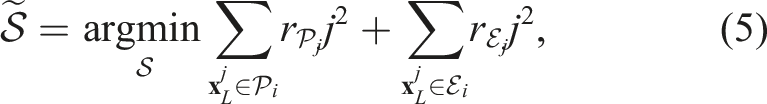
Abstract
This paper introduces 2Fast-2Lamaa, a lidar-inertial state estimation framework for odometry, mapping, and localization. Its first key component is the optimization-based undistortion of lidar scans, which uses continuous IMU preintegration to model the system’s pose at every lidar point timestamp. The continuous trajectory over 100–200 ms is parameterized only by the initial scan conditions (linear velocity and gravity orientation) and IMU biases, yielding eleven state variables. These are estimated by minimizing point-to-line and point-to-plane distances between lidar-extracted features without relying on previous estimates, resulting in a prior-less motion-distortion correction strategy. Because the method performs local state estimation, it directly provides scan-to-scan odometry. To maintain geometric consistency over longer periods, undistorted scans are used for scan-to-map registration. The map representation employs Gaussian Processes to form a continuous distance field, enabling point-to-surface distance queries anywhere in space. Poses of the undistorted scans are refined by minimizing these distances through non-linear least-squares optimization. For odometry and mapping, the map is built incrementally in real time; for pure localization, existing maps are reused. The incremental map construction also includes mechanisms for removing dynamic objects. We benchmark 2Fast-2Lamaa on over 750 km of public and self-collected datasets from both automotive and handheld systems. The framework achieves state-of-the-art performance across diverse and challenging scenarios, reaching odometry and localization errors as low as 0.22% and 0.06 m, respectively. The real-time implementation is publicly available at https://github.com/clegenti/2fast2lamaa.
1. Introduction
Over the past decades, the robotics community has put a lot of effort into solving odometry, that is, estimating a system’s ego-motion in unknown environments. In our previous work (Le Gentil et al., 2025), we showed that modern sensing capabilities provide highly accurate odometry even in challenging automotive scenarios. For the majority of real-world robot deployments, odometry alone is not sufficient to estimate the system’s state. With the example of self-driving vehicles or autonomous conveying, the robot is expected to navigate between known locations in a previously mapped environment. In this context, the critical enabling component for autonomous operations is localization, not odometry. The latter is simply used as an initial guess/prior between localization steps. In this paper, we present 2Fast-2Lamaa, which stands for Fast Field-based Agent-subtracted Truly coupled Lidar Localization and Mapping with Accelerometer and Angular-rate. This convoluted acronym refers to a lidar-inertial framework that addresses both mapping and localization by tightly coupling lidar and inertial measurement unit (IMU) measurements and leveraging continuous distance fields to represent the environment.
The first step of most lidar-based systems is motion-distortion correction. Commonly used lidars do not capture instantaneous snapshots of the environment; instead, they sweep one or more laser beams through the scene to collect 3D scans. Accordingly, any motion of the sensor during a scan’s duration creates motion distortion in the data. Many lidar-based state estimation algorithms leverage data from an IMU to address this issue (Lee et al., 2024). The most naive approach consists of using the latest pose and velocity estimates and integrating the inertial measurements to approximate the system’s trajectory for the duration of the incoming scan. With that movement prediction, the scan can be undistorted before being used in a non-linear optimization for scan-to-scan or scan-to-map rigid registration, alongside inertial constraints between consecutive scans. While this approach has been qualified as ‘tightly-coupled’ lidar-inertial estimation, for example, by Ye et al. (2019), this undistortion strategy is a ‘one-off’ operation that can be thought of as an ‘open-loop’ process. Because it freezes the scans based on prior information, it decouples the problem of lidar data undistortion from the estimation of scan-to-scan motion. This can lead to unrecoverable errors if the prior state estimate is not accurate enough due to accumulated drift or outlier data. Other approaches to lidar-inertial state estimation consider the lidar points individually through some continuous motion representation. There, the IMU measurements can be used as residuals to constrain the continuous state (Talbot et al., 2025) or directly used to locally parameterize the trajectory (Le Gentil et al., 2018). These methods estimate the system’s trajectory at the same time as correcting motion distortion in a truly coupled manner. Building upon our previous work (Le Gentil et al., 2024a), 2Fast-2Lamaa falls into the latter category by fully characterizing the trajectory during a scan based on IMU measurements without the need for any explicit motion model.
Once a scan is undistorted, 2Fast-2Lamaa performs localization by estimating a rigid transformation through scan-to-map registration. Note that when used for odometry or mapping, 2Fast-2Lamaa builds the map incrementally, whereas it leverages a previously built map when performing pure localization. A key component of a localization framework is the choice of map representation. The majority of lidar-based state estimation frameworks model the environment with point clouds (with or without normal vectors). In such a case, scan registration is generally performed with a variant of the iterative closest point (ICP) algorithm (Besl and McKay, 1992). 2Fast-2Lamaa differs from this paradigm as it leverages distance fields. These are continuous functions that can be queried at any location and that return an approximation of the Euclidean distance to the closest object/surface in the environment. Accordingly, the registration process consists of directly minimizing distance queries in a non-linear least-squares formulation, neither requiring explicit geometric primitives to model the environment nor any data association steps. The distance field presented in this work is based on Gaussian process (GP) regression (Rasmussen and Williams, 2006), similarly to Le Gentil et al. (2024b). While the concept of a GP-based distance field is not new, 2Fast-2Lamaa is the first real-time state estimation framework that successfully builds upon this idea for large-scale operations (sequences over 10 km-long), as illustrated in Figure 1. Note that this integration is not trivial, as standard GP regression suffers from cubic computational complexity. By leveraging efficient data structures and computing GPs locally, 2Fast-2Lamaa’s novel distance field approximation displays a log(N) computational complexity. The efficient data structures also enable real-time dynamic object removal through simple ray tracing. 2Fast-2Lamaa performs odometry, mapping, and localization over large-scale environments. It relies on GP-based distance fields for scan-to-map registration. Thanks to efficient data structures, the map can contain details of the environment’s geometry while allowing large-scale operations. The images here are visualizations of the map created with an 8 km-long Suburbs sequence from the Boreas-RT dataset. Despite the length of the trajectory, the map can represent all the observed geometry (a), without sacrificing details (b).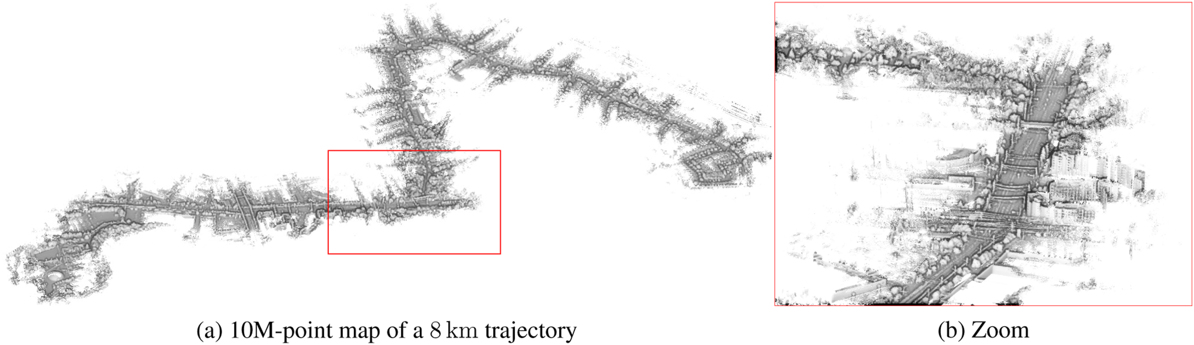
Regardless of the choice of geometric representation (point cloud, mesh, distance field, etc.), mapping and localization frameworks can opt for different high-level mapping strategies. The most natural option is to use a single globally consistent map. However, it has been demonstrated that accurate localization does not require geometrically consistent global maps (Baumgartner and Skaar, 1994; Brooks, 1987). Using a topometric approach that only requires local geometric consistency, Furgale and Barfoot (2010) performs navigation by moving in a set of topologically connected submaps, alleviating the need for perfect odometry/trajectory estimation when building the map. This approach is especially suited for Teach and Repeat tasks, where the robot is manually piloted to map the environment (teach/mapping) before performing autonomous path tracking to follow the original trajectory (repeat/localization). Our proposed framework can operate with either a globally consistent map or in a topometric manner, utilizing a succession of submaps to localize the robot’s repeating trajectories.
As any odometry pipeline is bound to drift, building maps purely on odometry estimates lead to inconsistencies at the global scale when considering trajectories that include loops that revisit previously explored areas. While not the core focus of the present work, 2Fast-2Lamaa can also be used for globally consistent trajectory estimation by performing loop-closure detection and batch pose-graph optimization, similarly to simultaneous localisation and mapping (SLAM) frameworks. This process is performed online when running odometry with submaps (topometric mapping mode). The proposed loop-closure detection and correction pipeline relies on the projection of each submap into 2D image-like data structures that represent the environment’s elevation changes. Similar to the work by Giubilato et al. (2022), visual features are extracted from these image-like structures, matched to detect loop-closures, and then used to provide the associated rough SE(2) geometric transformation between submaps. After SE(3) submap-to-submap pose refinement with the aforementioned GP-based distance fields, the global pose of each submap is estimated in a batch pose-graph optimization.
To summarise, our contributions are: • The integration of truly coupled lidar-inertial motion-distortion correction in a localization and mapping framework named 2Fast-2Lamaa. • The development of an efficient GP-based distance field for large-scale online mapping in the presence of dynamic objects. • The integration of an online loop-closure detection and correction mechanism to extend 2Fast-2Lamaa’s capabilities beyond odometry and incremental mapping. • An extensive odometry and localization evaluation of 2Fast-2Lamaa with more than 750 km of automotive and handheld data. • An open-source real-time implementation.
2. Related work
2.1. Lidar state estimation
There are many different approaches to state estimation in the robotics literature. In this section, we mainly consider optimization-based lidar(-inertial) frameworks. The majority of such methods can be classified into three distinct state estimation categories illustrated in Figure 2: (a) discrete, (b) continuous, and (c) hybrid. As mentioned in the introduction, motion distortion is addressed differently depending on the state representation. The first one (a) dissociates the act of undistortion from state estimation. Thus, motion correction is an open-loop process that preprocesses the scans based on previous estimates, and state estimation is discretely solved at the starting timestamp of each scan. With (b) and (c), state estimation and motion distortion are coupled in a single problem that estimates the continuous trajectory of the sensor (at least locally). Fully continuous approaches (b) generally assume a certain motion model to represent the sensor’s movement with a continuous function. IMU measurements can be used as residuals or control inputs of the system’s trajectory. Hybrid approaches (c) attempt to leverage the best of both (a) and (b) by locally parameterizing the trajectory based on inertial information, while keeping discrete variables at the global scale for simplicity and computational efficiency. The rest of this subsection provides a brief literature review of the three types of methods. Most optimization-based lidar state estimation frameworks can be classified into three categories. (a) represents discrete-time estimation where the system’s pose is estimated at a finite set of timestamps. The trajectory between timestamps is not estimated. (b) leverages a function over the whole duration of operations to represent the motion continuously. Such a method generally relies on some motion model and is parameterized by a set of supporting points. (c) shows a hybrid approach that locally characterizes the trajectory continuously based on inertial data, but uses discrete state variables at the global scale. This approach does not require an explicit motion model, but the global trajectory shows discontinuities when switching to a new timestamp. 2Fast-2Lamaa is built on the latter paradigm.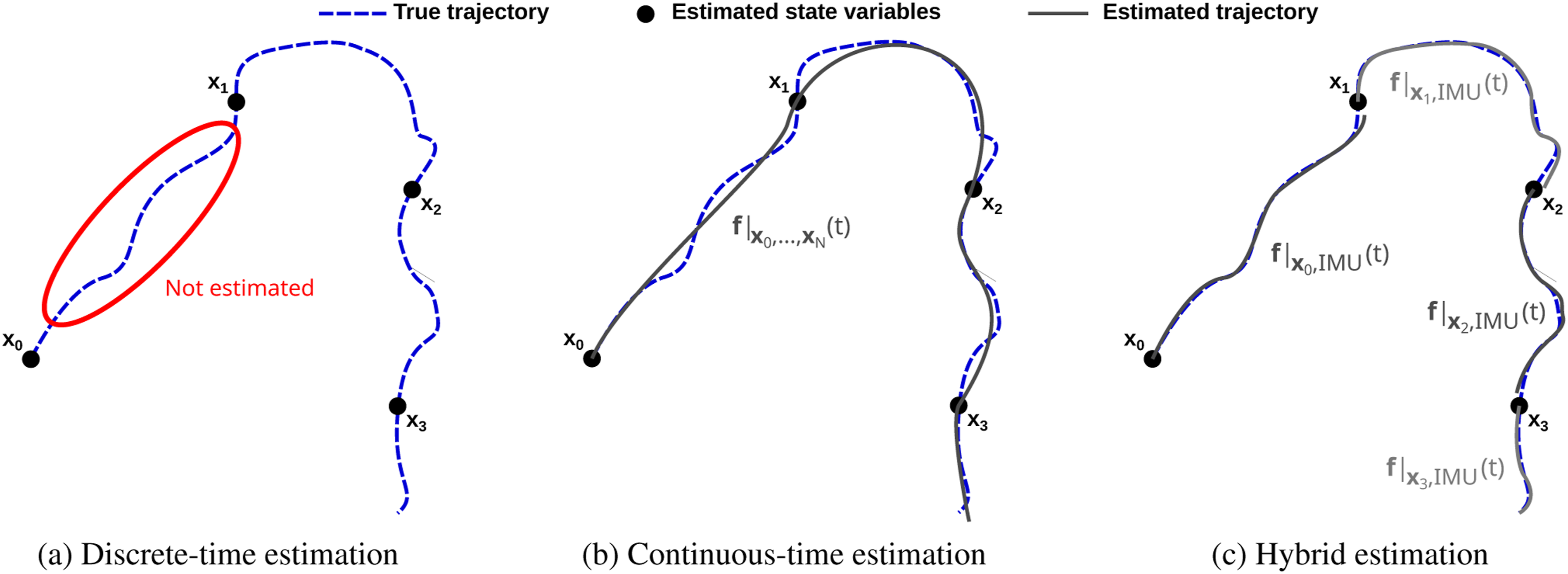
Considered as state-of-the-art odometry frameworks, Fast-LIO2 (Xu et al., 2022) and DLIO (Chen et al., 2023) are examples of one-off undistortion processes based on discrete-state estimation. The former uses an iterated Kalman filter, with the core registration step consisting of optimizing point-to-plane residuals between the open-loop-undistorted scans and a global map built incrementally. DLIO introduces a more precise way to undistort the point clouds using a constant-jerk motion model for continuous integration of the IMU measurements. After motion-distortion correction, DLIO performs a variant of Generalized-ICP (Segal et al., 2009) and uses a ‘hierarchical geometric observer’ (Lopez, 2023) to estimate the system’s pose efficiently. Note that DLIO and Fast-LIO2 only optimize for the last sensor pose. Other works leverage a similar undistortion process but optimize over a window of poses in a factor-graph formulation (Shan et al., 2020; Ye et al., 2019). Note that the aforementioned frameworks require sufficient geometric features in the system’s surroundings. To address geometrically degenerated environments, COIN-LIO (Pfreundschuh et al., 2024) proposes to leverage intensity information from the lidar data to extract distinctive features even on flat surfaces. More discrete-state lidar-inertial pipelines are discussed in a recent survey paper (Lee et al., 2024).
As shown in another recent survey paper (Talbot et al., 2025), there is a wide variety of continuous-time state formulations for robotics. Some of the early lidar(-inertial) work built upon continuous-time representations that make strong assumptions about the motion. For example, Zebedee (Bosse et al., 2012) uses piece-wise linear functions to model the system’s trajectory. This corresponds to a strict assumption of constant velocity between control points. Using inertial residuals, it demonstrated the ability to map a 3D environment using a randomly oscillating 2D lidar. Later, LOAM (Zhang and Singh, 2014) used the same constant velocity assumption with both actuated 2D and 3D lidars. This assumption is still used in recent frameworks like CT-LIO (Dellenbach et al., 2022) or MOLA (Blanco-Claraco, 2025). A key contribution of LOAM was the introduction of planar and edge features extracted from the raw lidar data for efficient registration. This concept has been reused in many works, including LeGo-LOAM (Shan and Englot, 2018) and the present work (using a different extraction method).
Throughout the years, other continuous representations have been used to model more complex lidar trajectories. A recurrent formulation is based on splines (Cao et al., 2025; Droeschel and Behnke, 2018). The benefit of splines with respect to discrete state variables has been demonstrated in the context of vision-based SLAM by Cioffi et al. (2022) at the cost of a higher computational cost. Another branch of continuous-time estimation is based on a particular class of sparse GPs (Barfoot, 2024). This approach elegantly models the trajectory based on a probabilistic motion model. For both lidars and radars, continuous GP states with a white-noise-on-acceleration motion prior have demonstrated high levels of accuracy and real-time computation (Burnett et al., 2025a). Note that different motion priors are possible, as demonstrated by Tang et al. (2019) with a white-noise-on-jerk prior. And inertial data can also be used as control inputs (Burnett et al., 2025b; Lilge and Barfoot, 2025).
The hybrid approach shown in Figure 2(c) relies on IMU measurements to locally represent the system’s trajectory. An issue with inertial-based motion prediction/characterization is the strong dependence on initial conditions and biases when integrating and double-integrating the gyroscope and accelerometer measurements. To prevent the reintegration of the IMU data every time the initial conditions are updated during the state optimization process, Lupton and Sukkarieh (2012) introduced the concept of preintegration. It corresponds to the creation of pseudo-measurements that combine the information from multiple IMU measurements without the need to know the initial conditions. Numerous works have improved on the original preintegration method (Eckenhoff et al., 2019; Forster et al., 2017; Yang et al., 2020). The inertial chapter of the SLAM Handbook provides an overview and comparison of several of these works (Huang et al., 2026). Note that, unlike the original preintegration use case, the hybrid state estimation approach does not attempt to combine IMU measurements into a small number of pseudo-measurements but rather requires an ‘upsampling’ of the inertial information for it to be available at any timestamp. This approach was originally introduced to address the issue of lidar-IMU extrinsic calibration by first upsampling the raw inertial readings before performing preintegration at a higher frequency (Le Gentil et al., 2018). Later approaches elegantly addressed preintegration under the scope of continuous state representation (Le Gentil et al., 2020b; Le Gentil and Vidal-Calleja, 2023), enabling full-batch lidar-inertial localization and mapping (Le Gentil et al., 2021). As this hybrid approach is well-suited to asynchronous inertial-aided estimation, other works with event cameras (Le Gentil et al., 2020a; Li et al., 2024) and radars (Hatleskog et al., 2025) have adopted preintegration as their state representation. 2Fast-2Lamaa also uses continuous preintegration to characterize the system’s motion during each lidar scan. The corresponding discrete state is the gravity vector orientation, the linear velocity at the beginning of the scan, and the IMU biases, resulting solely in 11-degree-of-freedom (DoF) to optimize.
2.2. Map representation
Traditionally, robotic maps consist of geometric landmarks jointly estimated with the system’s pose (Dissanayake et al., 2001). Over the past decades, we have seen a constant increase in sensor bandwidth and computational power. Naturally, the robotics community has harnessed these new hardware capabilities with algorithms that build and use denser and denser maps of the environment. Nowadays, the most common representation for lidar state estimation consists of voxel maps where each cell stores the centroid and normal vector of all the points that occurred in the cell. Fast-LIO2 (Xu et al., 2022) is an example of such methods, leveraging point-to-plane registration constraints. Other works, such as KISS-ICP (Vizzo et al., 2023) and KISS-SLAM (Guadagnino et al., 2025), chose to use point-to-point residuals, but suffer from significantly lesser performance on benchmarks such as the Newer College dataset (Ramezani et al., 2020). Other frameworks keep more information in each cell, for example, the local distribution of the points with normal distributions (Biber and Strasser, 2003; Magnusson, 2009). Another way to model the environment is to use sets of surface primitives. Surfels might be the simplest of these primitives and have been used in numerous lidar frameworks (Bosse et al., 2012; Droeschel and Behnke, 2018; Park et al., 2018). Some recent works deal with more complex primitives by directly building and using a mesh of the environment (Lin et al., 2023; Ruan et al., 2023).
The aforementioned representations (point clouds, surfels, meshes, etc.) store information about the environment’s surface. While memory-efficient, they contain limited information about the rest of the space explored by the system. Volumetric approaches, on the other hand, store information over the whole space and can track occupancy, truncated signed distance field (TSDF), etc. These are less explored for lidar-based estimation, but are crucial for autonomous navigation (e.g. to plan safe trajectories through the environment). Voxblox (Oleynikova et al., 2017) and FIESTA (Han et al., 2019) are prime examples of such mapping techniques. Leveraging advances in computer graphics, many mapping frameworks have been built atop the OpenVDB structure (Museth, 2013; Museth et al., 2013). Some fuse information from multiple scans at the TSDF level (Vizzo et al., 2022), where others use the occupancy (Zhu et al., 2021), or the Euclidean distance field (Wu et al., 2025). Focusing on state estimation, VoxGraph (Reijgwart et al., 2020) extends VoxBlox (Oleynikova et al., 2017) and achieves real-time performance. It leverages SDF submaps to compute submap-to-submap pose constraints, which are then integrated into a pose-graph optimization framework. More specific to lidar systems, D-LIO (Coto-Elena et al., 2026) uses a fast truncated distance field stored in a multi-level hashmap to perform scan-to-map registration. While the authors claim scalability to large-scale environments, their experiments on the VBR dataset (Brizi et al., 2024) show a large RAM requirement that cannot be fulfilled without removing information from memory. Another interesting work is shown by Boche et al. (2025) with OKVIS2-X, where vision-based estimation can be complemented with lidar-to-occupancy-map factors (Boche et al., 2024) using the Supereight2 data structure (Funk et al., 2021). Focusing on exploration, Schmid et al. (2021) also leverage volumetric mapping with a submap-based strategy to account for large state estimate drift.
With the democratization of GPU computing, many robotics works have explored the use of neural representations and Gaussian splatting for map representation. Point-SLAM (Sandström et al., 2023) and Gs-icp SLAM (Ha et al., 2024) are examples of both approaches for SLAM with RGB-D sensors. DeepSDF (Park et al., 2019) proposes an auto-decoder architecture to learn and infer the signed distance function at object-scale. Later, iSDF (Ortiz et al., 2022) demonstrates the ability to model and learn such a field online for room-scale environments. While less popular, neural representations can be used for lidar-based state estimation. LocNDF (Wiesmann et al., 2023) addresses the localization problem with a neural field close to a TSDF, but cannot be run at sensor framerate, even in small-scale environments, while Nerf-LOAM (Deng et al., 2023) performs odometry and mapping in large-scale environments. More recently, PIN-SLAM (Pan et al., 2024) showcases top performance on the VBR dataset (Brizi et al., 2024) via TSDF modelling with real-time operations. PINGS (Pan et al., 2025) builds upon PIN-SLAM by coupling Gaussian splats with neural distance fields for improved rendering capacities using both lidar and vision-based sensing.
2Fast-2Lamaa follows a line of work that mixes both surface-based and volumetric information. Similar to the former, it only stores information on the surface of elements in the environment, but allows for the query of a Euclidean distance field approximation over the whole space without large memory requirements. This trend originated from the goal of surface reconstruction with GP implicit surfaces (Williams and Fitzgibbon, 2006), which models a signed distance field close to the objects’ surface. Later, Wu et al. (2021) show the ability to approximate the distance to the closest surface anywhere in space by applying a non-linear operation over a GP-inferred field. It is demonstrated with offline experiments that such GP-based approaches enable lidar state estimation and planning (Wu et al., 2023). Le Gentil et al. (2024b) significantly improve the distance approximation while alleviating the original tradeoff between accuracy and surface interpolation. It represents the foundation of the fast distance field derived in the present work, which does not consider a single and inefficient GP, but breaks down the distance field modelling into many small local GPs. Consequently, our new field formulation enables registration in kilometre-long maps in real time. In contrast, the original work by Le Gentil et al. (2024b) can barely run object-level odometry at 2 Hz.
2.3. Dynamic object rejection
A common assumption of many robotic state estimation algorithms is to consider the system’s environment to be static. This assumption is very rarely verified in real-world applications. While robust techniques like RANSAC or m-estimators enable a robot to deal with a certain level of dynamicity in the scene (considering dynamic object points as outliers), there has been a growing interest in performing dynamic object detection to create maps that only contain static elements (Duberg et al., 2024; Falque et al., 2023; Jia et al., 2024a; Schmid et al., 2023; Wu et al., 2024; Yoon et al., 2019). However, most methods that focus on state estimation in dynamic environments first classify the points before performing standard scan registration (Pfreundschuh et al., 2021), and optionally tracking objects (Jia et al., 2024b). Other methods simply detect dynamic objects after lidar data registration (Le Gentil et al., 2024a; Lichtenfeld et al., 2024), relying on robust estimators to ‘ignore’ dynamic objects during the scan-alignment process. An exception to these two-step approaches is BTSA (Chen et al., 2025), which introduces a dynamic-aware ICP algorithm that couples the problems of dynamic point detection and state estimation in a single process. Another method, HiMo (Zhang et al., 2025), does not address the problem of ego-motion distortion, but tackles the moving object point cloud undistortion through scene flow estimation. We refer the reader to the relevant chapter of the SLAM Handbook (Schmid et al., 2026) for a deeper dive into state estimation in dynamic and deformable environments.
As the problem of dynamic object detection is not the core focus of 2Fast-2Lamaa, the proposed optimization-based motion-distortion correction step relies on robust loss functions to consider dynamic objects as outlier information. However, after scan-to-map registration, dynamic points can be removed from the map in an online or offline manner through some sort of ray tracing, similarly to the work from Pomerleau et al. (2014). In our ablation study, we evaluate the impact of the presence of dynamic points in the map on localization.
3. Framework overview
Let us consider a 6-DoF IMU (3-axis gyroscope and 3-axis accelerometer) and a 3D lidar rigidly mounted together. The lidar collects 3D points denoted as 2Fast-2Lamaa consists of two functional blocks. The first one is an optimization-based motion correction module that undistorts lidar scans using continuous IMU preintegration to characterize the system motion with only 11-DoFs. Once corrected, the scans are used for scan-to-map registration to estimate the global pose of the system.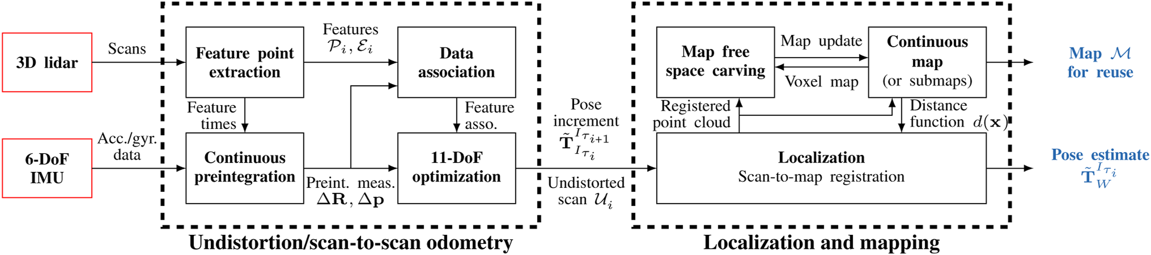
To undistort lidar scans, 2Fast-2Lamaa first extracts lidar features from the raw scans and performs continuous preintegration with the IMU data. Using continuous IMU preintegration, the system’s trajectory is parameterized by the gravity vector
For trajectory estimation, the localization module integrates the aforementioned incremental motion estimates and refines the global pose
4. Undistortion-based odometry
The undistortion module in 2Fast-2Lamaa is based on previous work for map-less and initialization-free dynamic object detection (Le Gentil et al., 2024a). The main differences are a novel approach for feature extraction and a change in the definition of the temporal window used for motion estimation. 2Fast-2Lamaa offers a faster front-end and reduces the time delay in the state computation by estimating the motion for the last incoming lidar scan, not waiting for subsequent scans as originally done.
4.1. IMU preintegrated continuous state
To undistort the incoming lidar data, let us consider the lidar points and IMU readings that have been collected over a short period of time. For convenience and implementation efficiency, this temporal window is chosen to span over two lidar scans (each defined as a full revolution for spinning sensors), with the previous scan from τi-1 to τ
i
and the current scan from τ
i
to τi+1. As formulated for SE(3) by Forster et al. (2017), the rotation, velocity and translation preintegrated measurements from time τi-1,
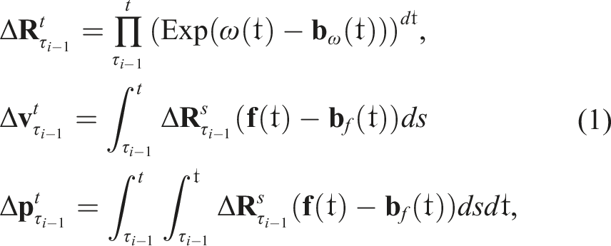
Note that the preintegrated measurements
4.2. Lidar features and data association
Using the raw lidar point clouds, features are extracted independently in the two scans that constitute the temporal window [τi-1, τi+1]. Similarly to the work by Zhang and Singh (2014), features can be planar or edge points. However, the feature point selection does not follow any type of curvature/roughness score. The planar points Accumulated lidar features (planar in green, edge in magenta) over 3 s of data in a Suburbs sequence from the Boreas-RT dataset.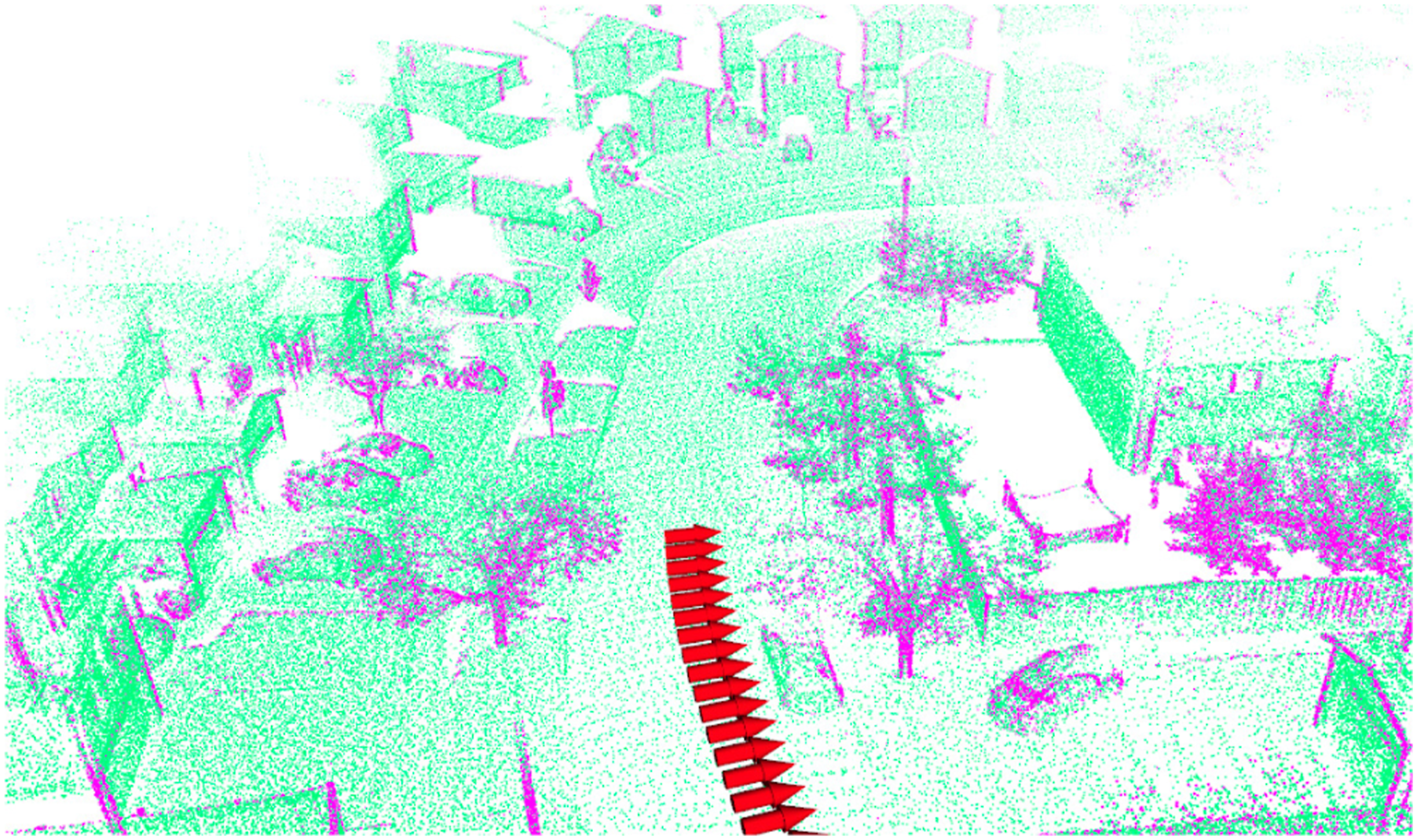
Then, the features from the two scans are associated together, between
4.3. Motion correction
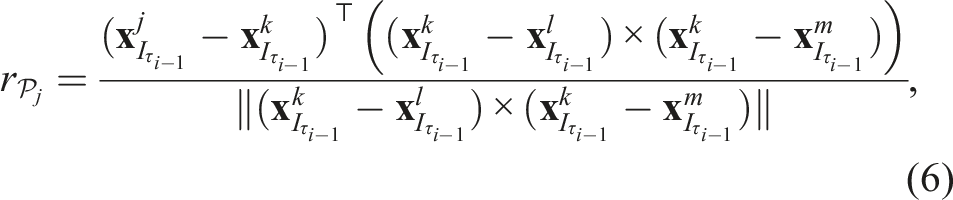
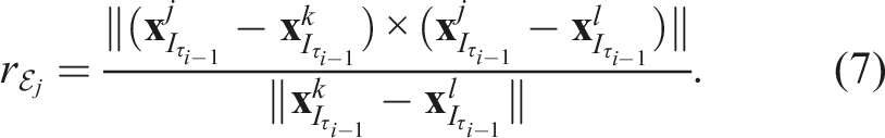
The motion is estimated via a non-linear least-squares optimization of point-to-plane and point-to-line distances
The undistortion process presented in this section is performed for every incoming scan and estimates the continuous trajectory between τi-1 and τi+1. It is done without fixing the motion between τi-1 and τ
i
in any way. Computing the motion for the duration of two scans at every scan creates an overlap in the consecutive temporal windows. That is why, at each step, the module solely outputs the transformation between τ
i
and τi+1, ignoring the estimate between τi-1 and τ
i
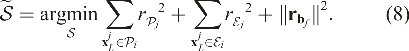
. It is important to note that the trajectory over a small temporal window (typically 200 ms) is often close to translation-only movement, or can be close to rotation-only in some scenarios. These motions are not informative enough to make the accelerometer observable, as there is an ambiguity with gravity, as detailed by Tereshkov (2015). To address this issue, a weak zero-mean prior residual
5. Localization
5.1. Scan-to-map registration
Given a motion-corrected point cloud
5.2. Gravity-alignment residual
Inspired by Noh et al. (2025), the scan-to-map registration (10) can be complemented with a gravity-alignment residual
Then, for any incoming undistorted scan and the associated linear body velocity
Finally, the gravity residual
5.3. Topometric localization
Atop localization in a globally consistent map, 2Fast-2Lamaa enables topometric localization (and mapping) for repeated robot operations along the same path. This is inspired by the Teach and Repeat framework (Furgale and Barfoot, 2010), which represents the environment with a graph of overlapping geometric submaps topologically linked based on a demonstrated robot trajectory. The localization process has two ‘layers’. At the high level, it consists of moving from submap to submap (node to node) in the topological graph. At the low level, it performs scan-to-submap geometric registration. This approach alleviates the need for a globally consistent map while allowing high-precision localization for autonomous navigation. We have integrated this mapping and localization strategy into the proposed framework. In its current version, 2Fast-2Lamaa only considers the simplest type of graph: an undirected chain. Concretely, the localization in that chain consists of performing scan-to-submap registration using (10) and the submap associated with the current node in the chain. Then, if the state estimate reaches the edge of the submap, the next node (or previous one, depending on the direction of motion) becomes the current node. Figure 5 illustrates a topometric map in the Suburbs environment of our self-collected dataset. While the trajectory used to create the map drifted from the ground-truth, the topometric nature of the localization enables accurate localization for repeating trajectories (<3 cm lateral position root mean squared error (RMSE); see Section 9.3). Example of topometric map obtained on a Suburbs sequence of the Boreas-RT dataset. It consists of a succession of submaps (shown as point clouds of different colours) and a topological graph (shown in red, with the sphere being the submaps’ centroids) that connects the submaps. This topometric map does not require global consistency to enable state-of-the-art localization in repeating trajectories.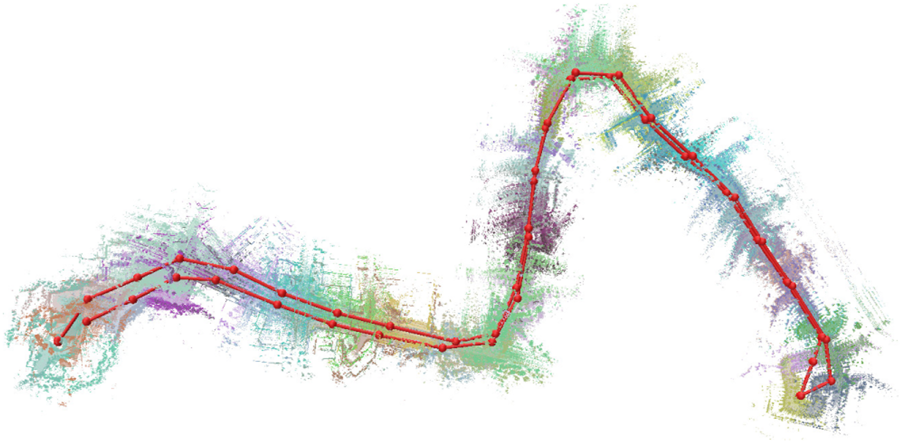
6. Mapping
This section presents the proposed GP-based distance field for efficient scan-to-map registration in Section 5. The map can be provided with a single point cloud of the robot’s environment or incrementally built according to the scan-to-map odometry estimates. The incremental map creation can be done using a single map or a collection of submaps for the topometric localization mode. The process presented in this section applies to all of these mapping strategies. The only difference for the topometric approach is that a new submap is created after a user-defined distance travelled since the last submap creation.
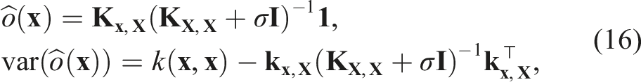
6.1. GP-based distance field
The proposed mapping process is based on GP-based distance fields (Le Gentil et al., 2024b). Using a point cloud as input, it performs standard GP regression to obtain a latent field o(


The definition of r depends on the kernel function k

With an unscaled, stationary, isotropic kernel (that can be written as a function of the distance k(
6.2. Efficient large-scale GP distance field
An issue with naively applying standard GP regression is the cubic computational complexity O(N3) with respect to the number N of points in the map due to the matrix inversion in (16). In this work, we propose a novel and efficient strategy for GP-based distance field by computing local GPs instead of a single global one. The core principle behind this strategy is the spatially limited impact of each input point due to the lengthscale of the kernel. 1 In other words, performing GP regression considering a large-enough local neighbourhood of points will (locally) yield a similar inferred mean when compared with using all the available observations.
The key to our approach is to leverage both a sparse voxelized representation
Integrating new points in the map simply consists of checking if the corresponding cell index is already present in the hashmap. If yes, the cell’s centroid is updated incrementally with the new point location. Otherwise, a new cell is created, and its position is added to the spatial index. Thanks to the hashmap properties, accessing an existing cell or inserting a new one is constant-time O(1) on average. The insertion of a new cell in a spatial index is slower with an O(log(N)) average complexity at best. Fortunately, thanks to the voxelized nature of the stored information, only a small portion of the incoming lidar points lead to cell creation (e.g. a 7.9 km-long suburban trajectory in the Boreas-RT dataset contains over 1.8 trillion lidar points, but the final number of cells in the map is around 10 million).
To query d(
There are two main caveats to the proposed field. The first is linked to the use of local GPs, creating a discrete behaviour when potentially switching from one local GP to the next while querying two locations that are side by side. In other words, the global field is not guaranteed to be continuous over the full space Illustration of the impact of the proposed weighting mechanism for our efficient GP-based distance field inference with sparse voxelized observations. The cell centroids are in red, and the colourmap represents the distance field (the colour is purposely saturated at 1 m for the sake of visibility. (a) is the inference with equal weight for each voxel observation. (b) is the inference with the proposed weighting based on the number of lidar points that occurred in each cell. One can clearly see the improvement in terms of smoothness and ‘wall thickness’, thus the accuracy of the field.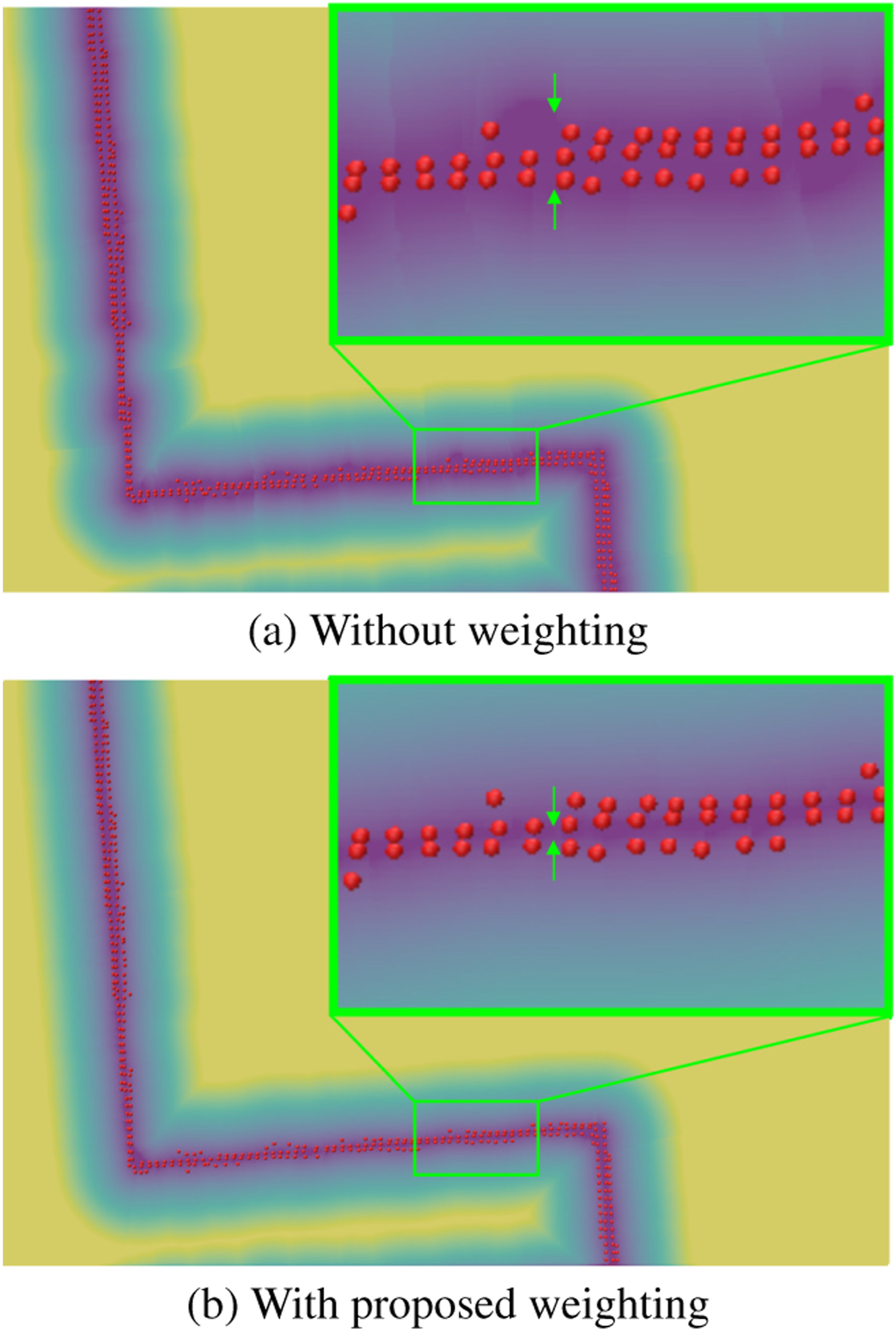
6.3. Free-space carving
In self-driving scenarios (among others), it is impossible to guarantee that the environment is static at the time of mapping. Thus, a mechanism for rejecting dynamic objects from the map can help build cleaner maps for later reuse in a localization-only phase. 2Fast-2Lamaa includes a free-space carving step to remove dynamic points previously inserted in the map and account for changes in the environment, such as parked cars that are no longer present. The principle of the proposed mechanism relies on the comparison between the spherical projection of the current scan and that of the map cells in the vicinity of the current sensor position. First, the scan is projected onto an image-like data structure by discretizing the azimuth and elevation of each point using a resolution of around 1°. Each pixel retains the range value of the closest point that is projected into it. Then, the map points within a radius around the sensor position are queried and projected in the aforementioned image-like data structure using spherical coordinates. If the range of a map point is smaller than the corresponding scan range, using a margin equal to the voxel resolution, it is removed from the map as it occurred between a surface currently observed and the sensor. Figure 7 illustrates this process with dense simulated data for the sake of clarity. Free-space carving can be performed online before inserting a freshly registered point cloud into the map, and offline by revisiting the whole trajectory and scans. Illustration of the free-space carving process of the proposed mapping framework (using Handa et al. (2014)’s living room simulated environment).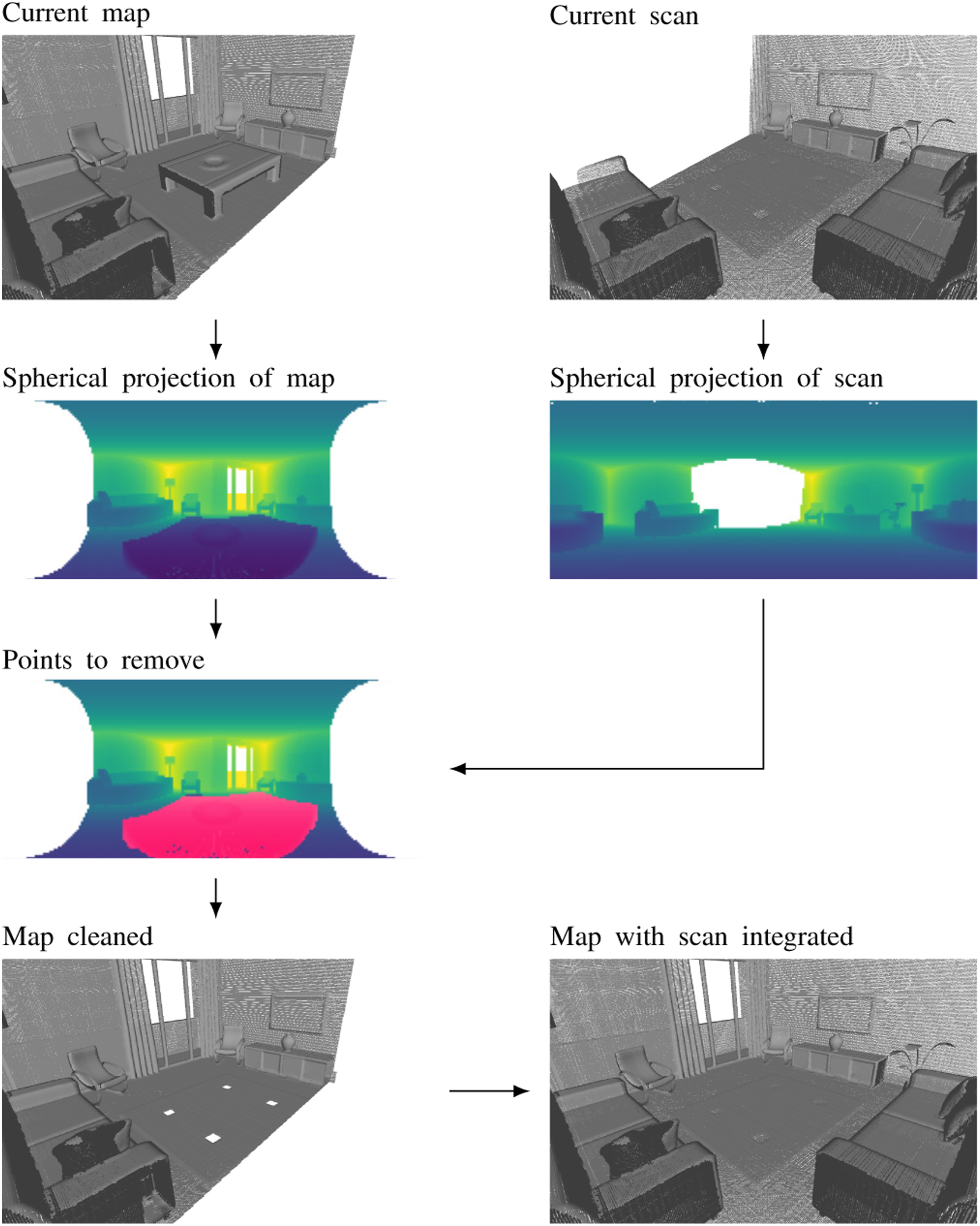
7. Online pose-graph optimization
When used in mapping mode with a single global map incrementally built based on odometry estimates, the proposed scan-to-map strategy cannot guarantee global consistency when the robot’s trajectory forms loops due to the inherent drift in any odometry algorithm. While using submaps in a topometric approach alleviates this issue for any robotic application that involves repeated motion (teach-and-repeat-like), one might be interested in obtaining a globally consistent trajectory for globally consistent mapping. Toward this goal, 2Fast-2Lamaa also integrates an optional3‡ online loop-closure detection and correction mechanism based on feature descriptor matching and pose-graph optimization, similar to the work by Giubilato et al. (2022).
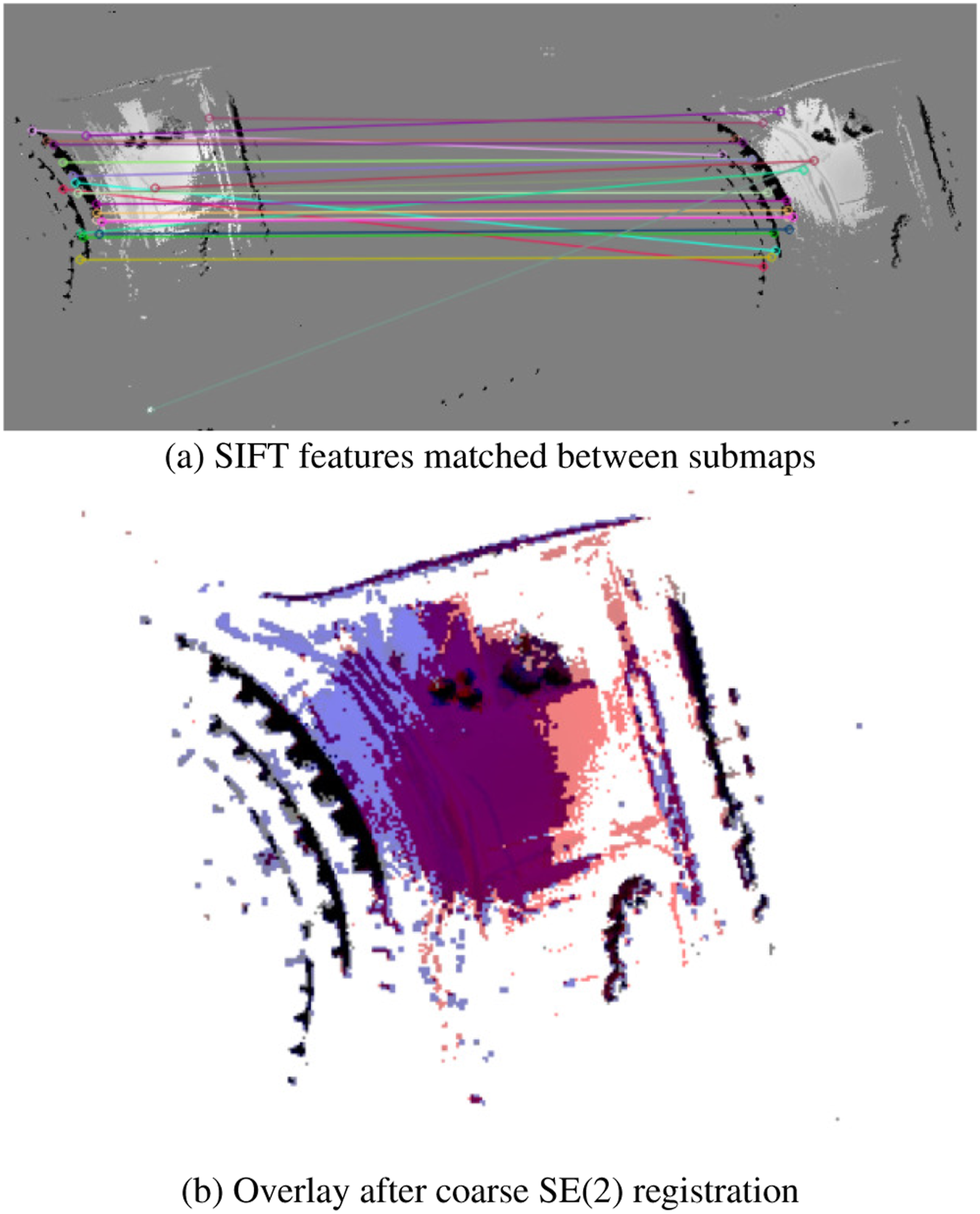
Figure 8 shows the proposed pipeline. First, 2Fast-2Lamaa’s topometric mapping mode is leveraged to obtain submaps and submap-to-submap transformation estimates Overview of the proposed loop-closure detection and correction based on the output of 2Fast-2Lamaa in topometric mapping mode. First, the 3D submaps are projected into image-like elevation gradient maps (2.5D). Using visual features, the 2.5D submaps are coarsely aligned by SE(2) RANSAC registration and elevation alignment. Thresholds on the number of inliers and the elevation coherence are used to discard non-loop-closure submap pairs. Based on the proposed GP-based distance field, coarse loop-closure transforms are refined before being used as residuals in a pose-graph optimization that leverages the odometry pose estimates between consecutive submaps. Illustration of the loop-closure detection and SE(2) registration used in our online pose-graph optimization of 2Fast-2Lamaa’s submaps. The proposed pipeline relies on the extraction, matching, and registration of visual features in image-like elevation representations of each submap.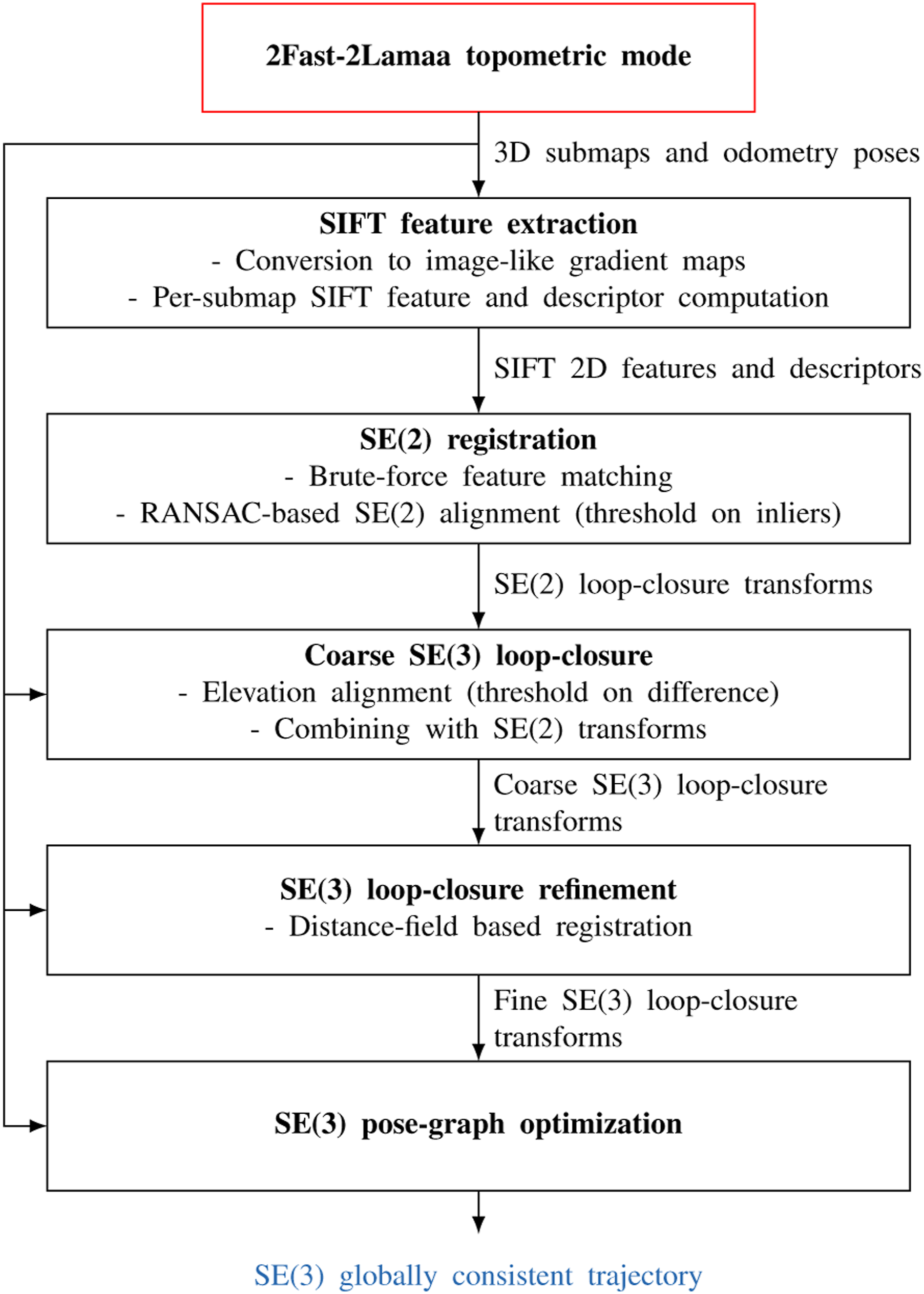
8. Implementation
In this section, we present and discuss some specific details of our ROS2 C++ implementation.
8.1. Low-level data structures
The hashmaps in the work use the
The constraints on the choice of the spatial index • Fast and scalable insertion of new elements. • Possibility to remove points without the need to recreate the index. • Allowing for N-closest neighbour and radius search.
The ikd-Trees (Cai et al., 2021), PH-Trees (Zäschke et al., 2014), and i-Octrees (Zhu et al., 2024) match the aforementioned requirements. Appendix A.3 shows a toy-example evaluation. We observed a significant advantage for the i-Octree. For efficiency, the spatial indexing structure is not updated with the changing centroid of the voxels, but the hashmap is. The spatial index relies on the coordinates of the first point that occurred in each voxel. Accordingly, the closest neighbour or radius searches performed with the ‘out-of-date’ spatial index are only approximations. We found this not to be a problem empirically, as the GPs are computed with the up-to-date voxel centroids of the local neighbourhood that is more than twice as large as the voxel resolution. For some specific scenarios, such as queries in the middle of a corridor, the query for the closest voxel in the spatial index, whether it is out-of-date or up-to-date, can erroneously trigger GP computations using points from the furthest of the two sides. A simple workaround is to perform K closest neighbour searches with associated local GP-based distance field computation for each query. The final distance would be the smallest of the K resulting GP-inferred distances. Note that this corridor-like scenario is unlikely when performing scan-to-map registration thanks to the accurate initial guess from 2Fast-2Lamaa’s undistortion module. Thus, our implementation uses K = 1 for registration. For other queries, the default is K = 2.
8.2. Non-linear optimizations
All the optimizations in this work (lidar-inertial undistortion and scan-to-map registration) are based on Ceres, an open-source non-linear least-squares solver (Agarwal and Mierle, 2022). Both (5) and (10) leverage Cauchy loss functions to attenuate the impact of outliers. The analytical Jacobians of the residuals are provided to the solver. To lower the computational cost of the overall pipeline, we adopted a basic keyframing strategy for the scan-to-map registration, performing (10) only when the sensor has moved sufficiently or after a fixed time period.
8.3. GP kernel and distance field
While it was shown that the square-exponential provides the best accuracy for distance field estimation (Le Gentil et al., 2024b), 2Fast-2Lamaa’s implementation uses the rational-quadratic kernel
8.4. Point-cloud filtering
Lidar data is generally not affected by different levels of luminosity in the environment. However, it can be degraded by floating particles in the air, such as dust or precipitation. To increase robustness in more challenging scenarios, 2Fast-2Lamaa offers the possibility to filter incoming point clouds based on the sensor-provided per-point intensity. While not thoroughly analyzed in this paper, we have observed a significant improvement of 2Fast-2Lamaa’s odometry and localization performance on the Farm sequences of the Boreas-RT dataset (Lisus et al., 2026), which were collected on an extremely dusty road. Additionally, a ‘density check’ is always performed on each undistorted point cloud in case the intensity filtering does not sufficiently remove amorphous point clusters. Using the user-provided map resolution, the scan is discretized into voxels. Points that fall into voxels that have more than twelve neighbours are ignored for registration.
8.5. Submapping strategy
When used with submaps, as opposed to building a single global map, 2Fast-2Lamaa uses a very simple submapping strategy: a scan is integrated in a submap if the sensor has travelled less than a user-defined distance γ since the submap creation. Note that the submaps overlap by a ratio β (equal to 0.2 in our experiments). Concretely, it means that a new submap is created when the distance travelled goes above (1 − β)γ. During the overlap, each scan is added to both submaps. When performing topometric localization, the change from one submap to the next is done when the current pose estimate is closer to the poses in the second half of the overlap than to the first half.
9. Experiments
We validate the proposed framework for both localization and odometry using various public datasets as follows: Section 9.2 uses the Boreas dataset; Section 9.3 is based on part of the Boreas-RT dataset; and Section 9.4 the Newer College dataset. We also leverage the VBR dataset for SLAM evaluation in Section 9.5. On top of this extensive benchmarking, we conduct an ablation using part of the Boreas-RT dataset in Section 9.6. Finally, Section 9.7 provides the reader with information about the computational requirements of 2Fast-2Lamaa.
9.1. Parameters
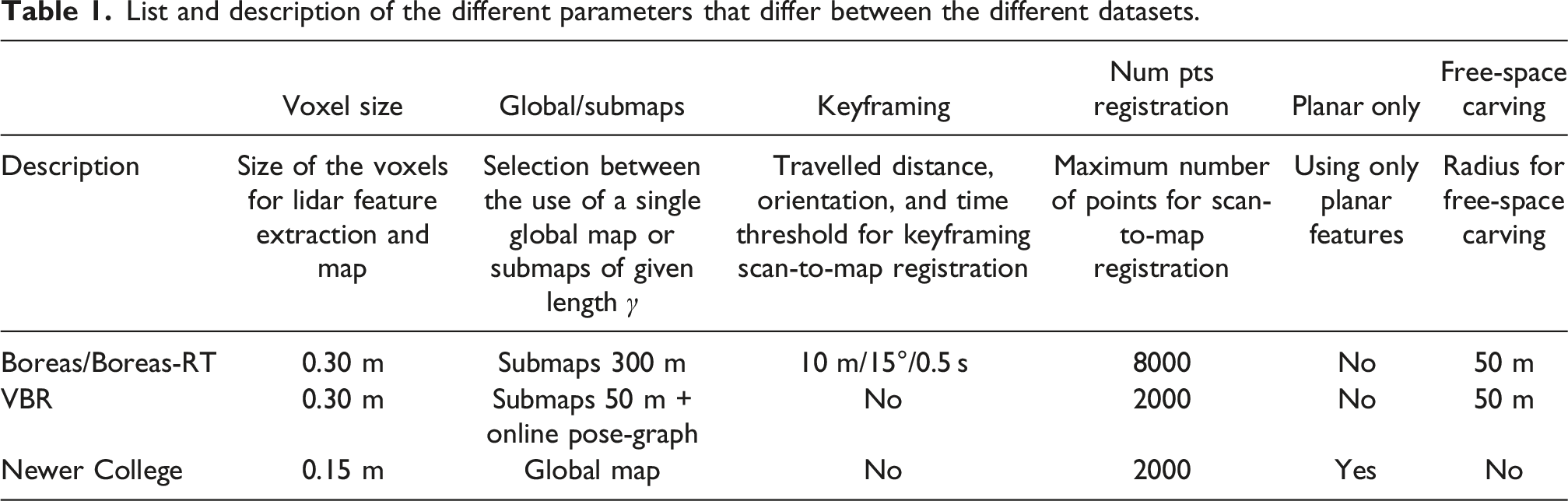
List and description of the different parameters that differ between the different datasets.
9.2. Boreas dataset
9.2.1. Dataset description
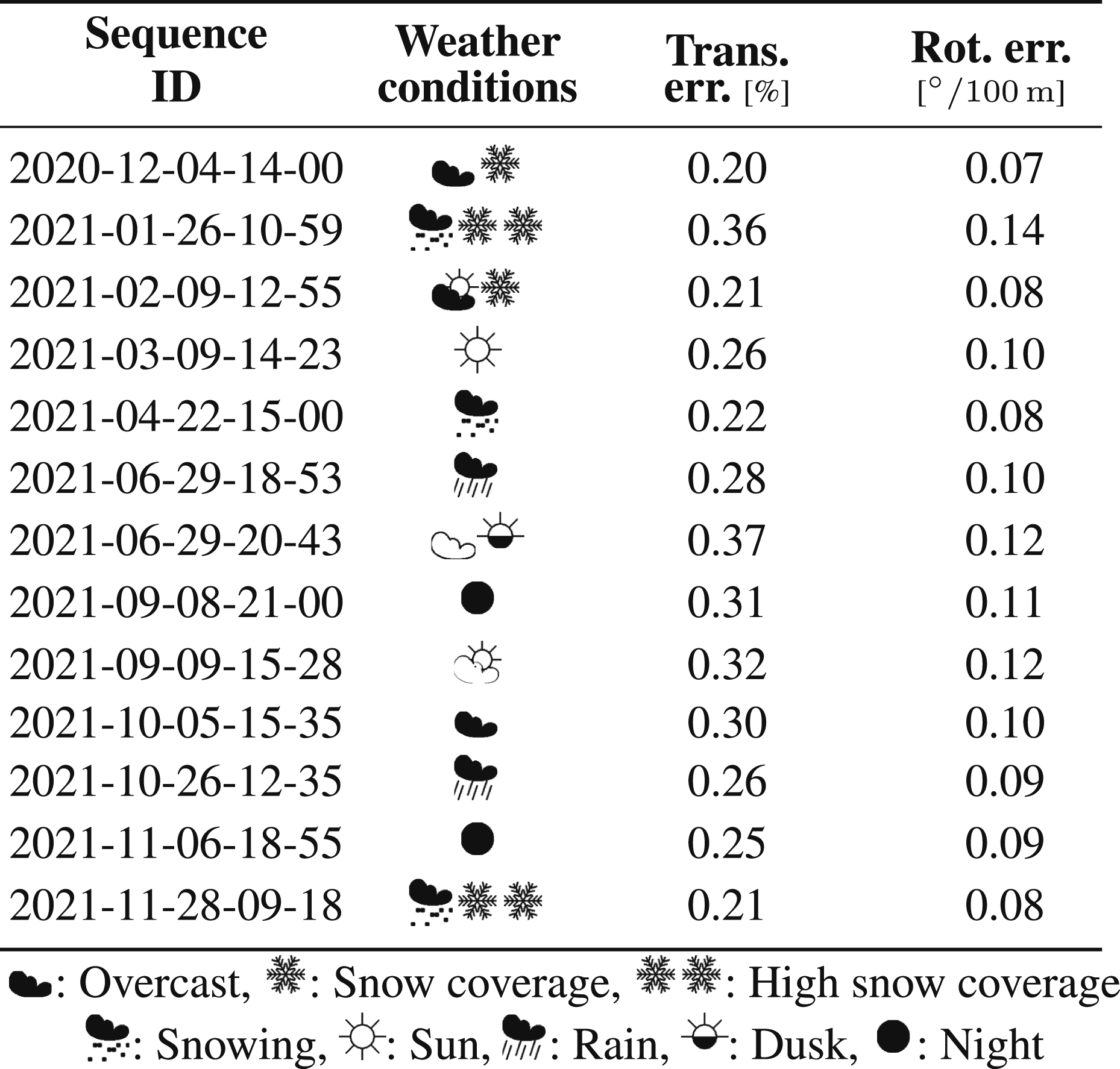
The Boreas dataset (Burnett et al., 2023) consists of 44 sequences collected along a single 8 km suburban route with an automotive sensing platform over the course of a year. The particularity of this dataset is the wide range of weather conditions in between different sequences, from bright sunny days to heavy rainfall and snowstorms. The vehicle is equipped with a Velodyne Alpha Prime lidar, a Navtech RAS6 imaging radar, a FLIR Blackfly S camera, and an Applanix RTK-GNSS-IMU ground-truthing solution. Figure 10 illustrates the impact of extreme weather conditions on lidar data. The Boreas dataset withholds the ground-truth trajectory for 13 of the 44 sequences, corresponding to more than 100 km of data collection. These are used to benchmark various state estimation methods with a public leaderboard. While not optimal due to data contamination between the ground-truth solution and the input of the various algorithms, the Applanix IMU is used in conjunction with the lidar in the rest of that section, as it is the only inertial sensor present aboard the vehicle. Impact of a snowstorm on the lidar data in the Boreas dataset (sequences 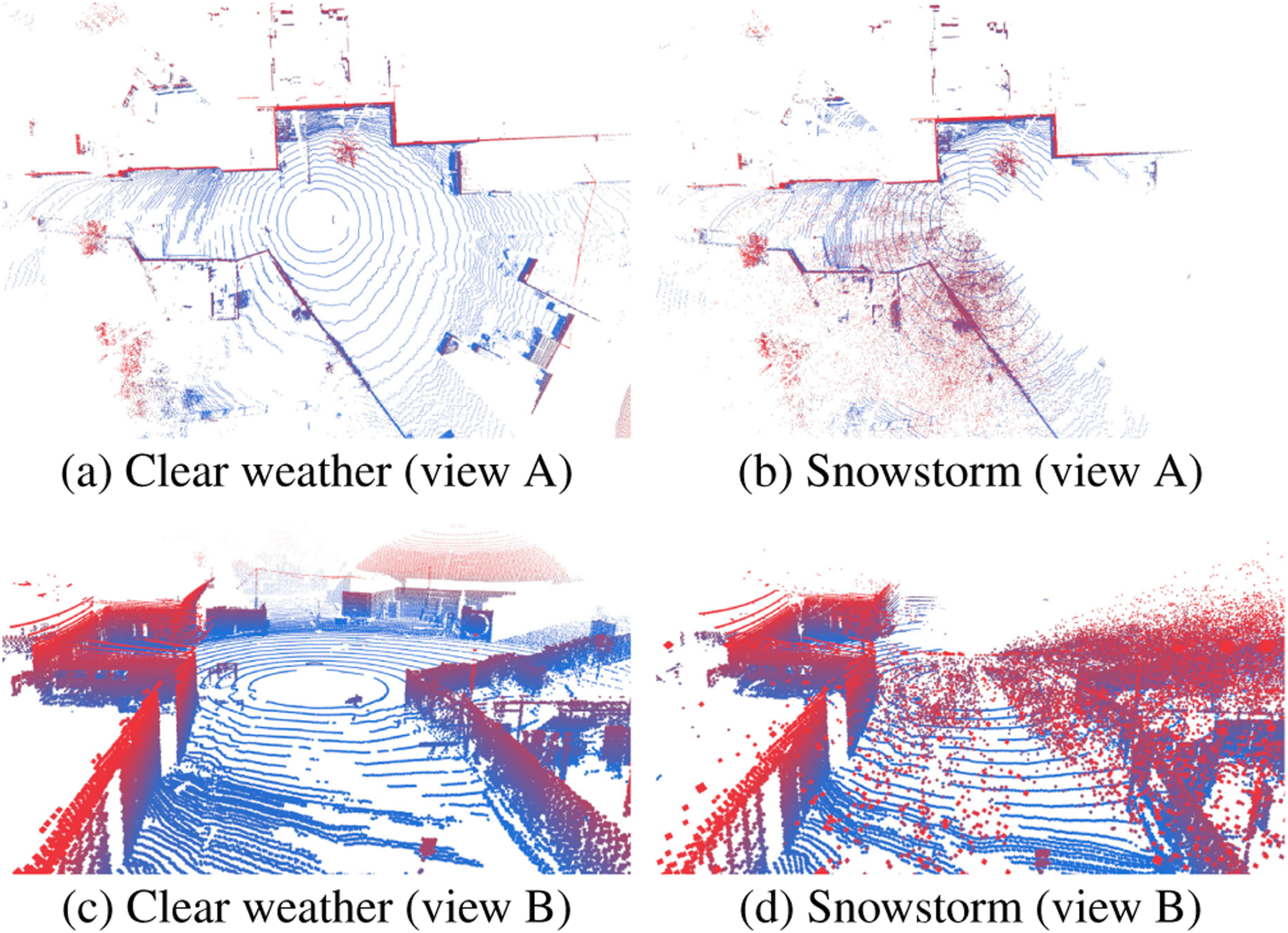
9.2.2. Baselines and metrics
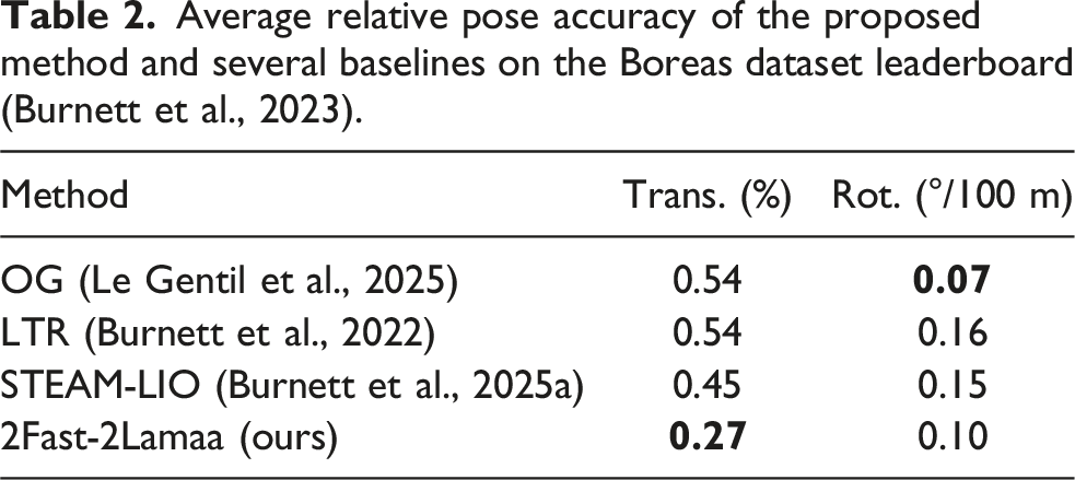
For odometry, we report the leaderboard’s KITTI odometry metric. Succinctly, this metric aligns trajectory chunks (every 10 lidar frames) of length (100 m, 200 m, …, 800 m) based on the first pose of each chunk, computes the error in position and orientation at the end of each segment, and reports the average translation and rotation error relative to the distance travelled. By submitting our results to the leaderboard, we benchmark our method against LTR (Burnett et al., 2022), STEAM-LIO (Burnett et al., 2025a), and OG (Le Gentil et al., 2025). Both LTR and STEAM-LIO are based on continuous-time ICP for lidar state estimation. The continuous trajectory formulation leverages efficient GPs with noise-on-acceleration motion priors. A major difference is the integration of inertial measurements in STEAM-LIO. The OG baseline does not use the lidar but solely the 3D gyroscope and wheel encoder. It represents the simplest and most efficient method for automotive odometry. Nonetheless, OG provides odometry accuracy on par with state-of-the-art exteroceptive frameworks.
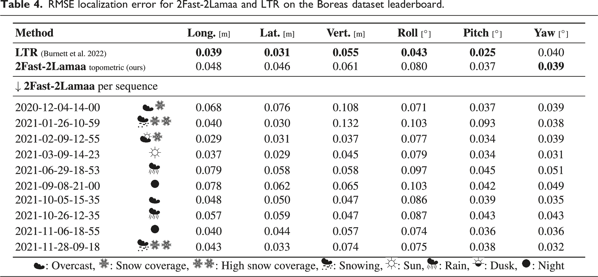
To assess the localization ability of 2Fast-2Lamaa, we leverage the localization part of the leaderboard. It consists of creating a map of the route given one sequence, and localizing within that map using 10 other sequences. The metric is the RMSE of the relative pose between the trajectory of the mapping sequence and the localization ones. Note that only LTR has been submitted to the Boreas benchmark (more baselines are used with a subset of the Boreas-RT dataset in Section 9.3). LTR’s strategy for localization is performing scan-to-local-map registration while accounting for past estimates and odometry in the form of a prior on the state.
9.2.3. Odometry benchmark
Average relative pose accuracy of the proposed method and several baselines on the Boreas dataset leaderboard (Burnett et al., 2023).
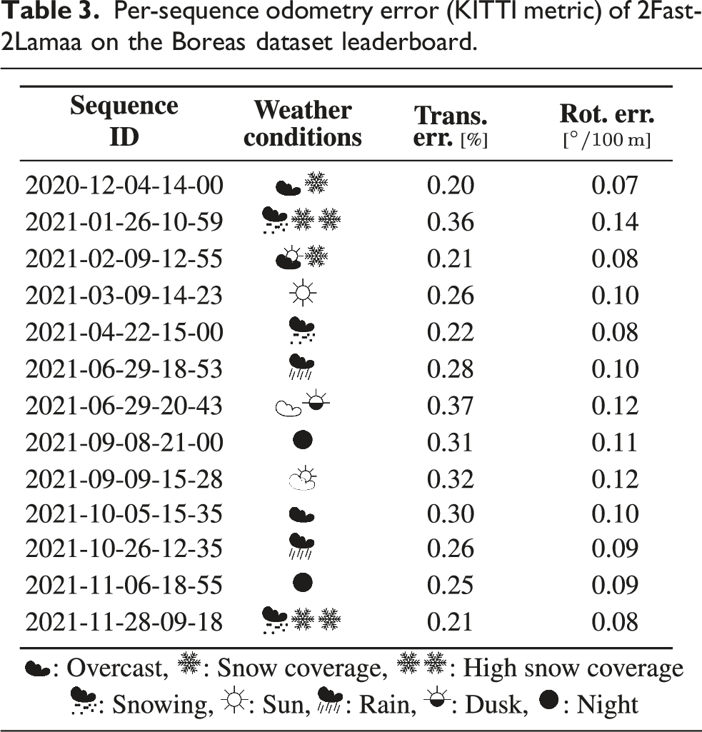
Per-sequence odometry error (KITTI metric) of 2Fast-2Lamaa on the Boreas dataset leaderboard.
9.2.4. Localization benchmark
RMSE localization error for 2Fast-2Lamaa and LTR on the Boreas dataset leaderboard.
9.3. Boreas-RT
9.3.1. Dataset description
To evaluate the proposed framework, we use data from the Boreas-RT dataset (Lisus et al., 2026). It uses the same sensing platform as the Boreas dataset with the main hardware differences being a different radar firmware and an additional 6-DoF Silicon Sensing DMU41 IMU to prevent data contamination between ground-truth and raw sensor data. In this section, we leverage 16 sequences in four different environments, totalling 120 km of data for benchmarking against various baselines. The different routes are Suburbs, Regional, Tunnel, and Skyway, listed in increasing level of difficulty. We also provide 2Fast-2Lamaa’s results on all of the 60 sequences of Boreas-RT (≈650 km) in Appendix A.4.
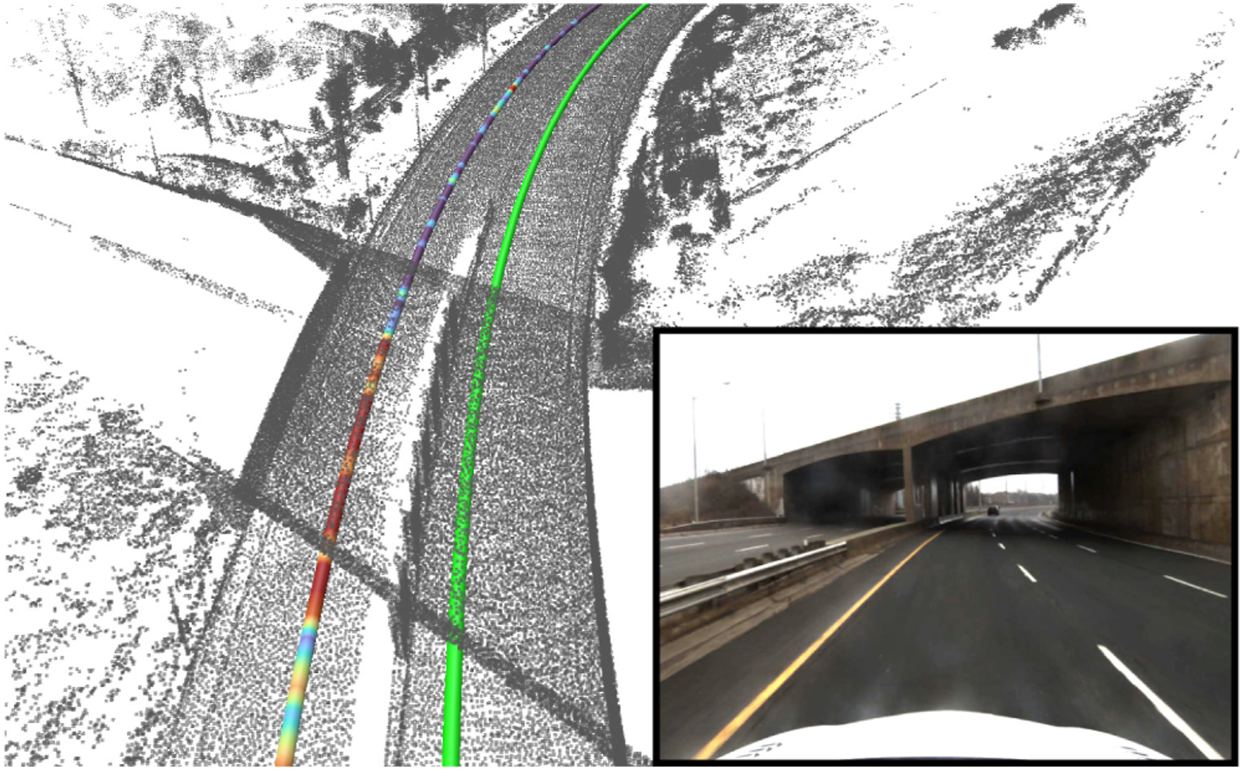
Suburbs sequences follow the same route as in the Boreas dataset. The road traffic varies between sequences, but a lot of geometric features are present in the surroundings. The Regional data is collected at a higher speed with fewer geometric features to constrain the vehicle’s pose. The Tunnel route goes through a kilometre-long tunnel with very few geometric features to leverage. Finally, the Skyway sequences go over a bridge/skyway with only a few lampposts as static features. A lot of the non-ground lidar points correspond to moving vehicles. Figure 11 provides images from the onboard camera as well as the OpenStreetMap overlay of the trajectories. Both the Suburbs and Skyway routes form loops, whereas Regional and Tunnel sequences do not revisit previously driven areas. The Regional data present an extra challenge for localization: the route is driven twice in each direction, thus, when mapping with one sequence and localizing with the other three, two of the localization runs experience quite different viewpoints than the one of the mapping step (cf. Figure 12). Similarly, the tunnel sequences are collected while driving in both directions. However, the tunnel consists of two separate tubes (one for each traffic direction) without co-visibility. Thus, our Tunnel localization experiments are run for each driving direction independently (two times: one sequence for mapping, one sequence for localization), and the quantitative results are the average of both. Images from the onboard camera of the Boreas-RT dataset and trajectory overlays (blue lines) on OpenStreetMap. The four Regional sequences have been collected in both directions (two each way). When mapping with one sequence, part of the environment is only visible from the opposite traffic lane, thus leaving gaps in the map (as illustrated here under a bridge, with the map in grey, and the mapping trajectory in green). This makes localization challenging: the second line represents the localization trajectory of the second sequence and is coloured with the localization error (purple low and red high).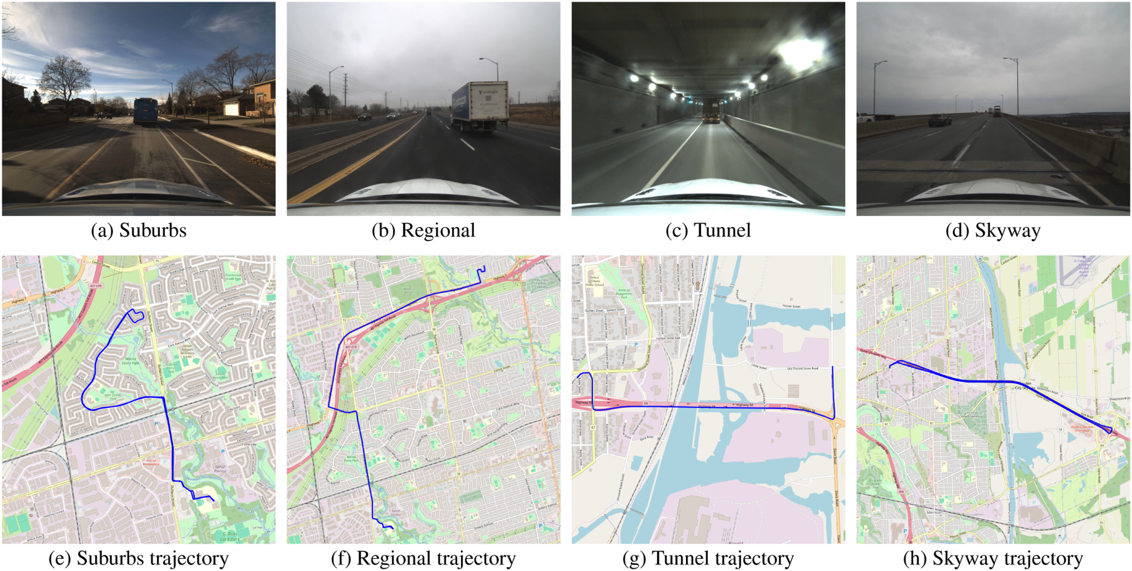
9.3.2. Baselines and metrics
The metrics used for odometry and localization are the same as for the Boreas experiments in Section 9.2. Regarding the odometry baselines, we benchmark 2Fast-2Lamaa against MOLA (Blanco-Claraco, 2025), Fast-LIO2 (Xu et al., 2022), and LTR with gyroscope (Burnett et al., 2022). Each of these method address motion distortion in a different manner: MOLA assumes strict constant velocity during each lidar scan (optimizing for the velocity at each ICP step), Fast-LIO2 undistorts the incoming data based on the previous estimate and the open-loop propagation of the IMU readings, and LTR performs fully continuous-time estimation with GPs. Note that the LTR version here is different from the one present on the Boreas leaderboard. The main difference is the integration of angular velocity readings from the gyroscope as extra factors in the continuous-time optimization. For evaluating 2Fast-2Lamaa’s localization abilities, we use LTR and Fast-LIO-localization (HViktorTsoi, 2020) as baselines. The latter is an open-source project that performs localization in maps built with Fast-LIO2.
Sensor-specific parameters are updated for each baseline. Our experiments with MOLA use the default algorithmic parameters from the public implementation. Fast-LIO2 does not expose algorithmic parameters to the user. For LTR, the parameters have been tuned for the best average performance. Fast-LIO localization has been tuned to limit the number of critical failures.
9.3.3. Odometry benchmark
Average relative pose accuracy of the proposed method and several baselines on a subset of the Boreas-RT dataset.
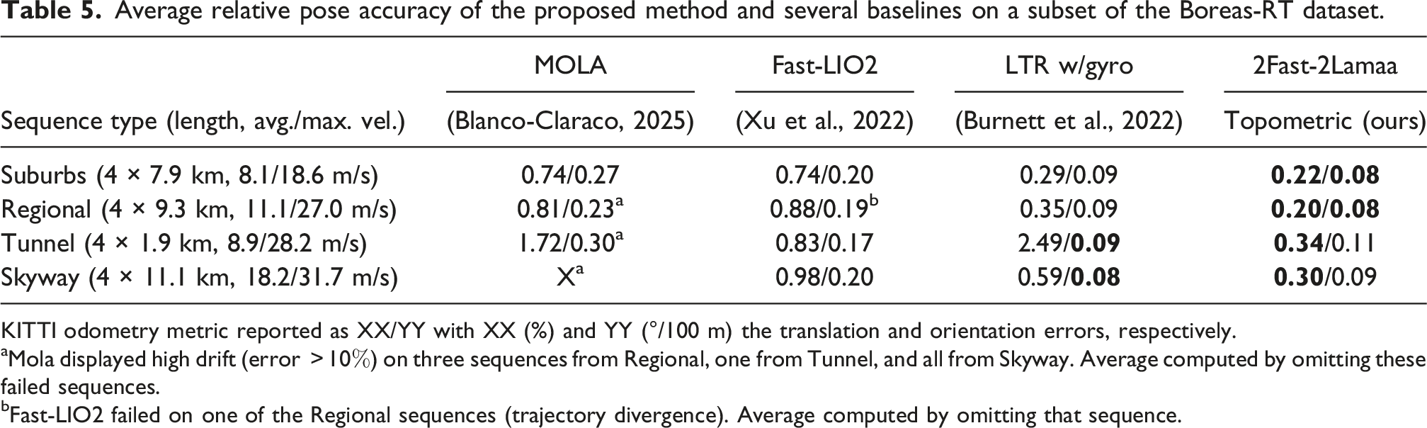
KITTI odometry metric reported as XX/YY with XX (%) and YY (°/100 m) the translation and orientation errors, respectively.
aMola displayed high drift (error
bFast-LIO2 failed on one of the Regional sequences (trajectory divergence). Average computed by omitting that sequence.
9.3.4. Localization benchmark
RMSE localization error for 2Fast-2Lamaa and different baselines on a subset of the Boreas-RT dataset.
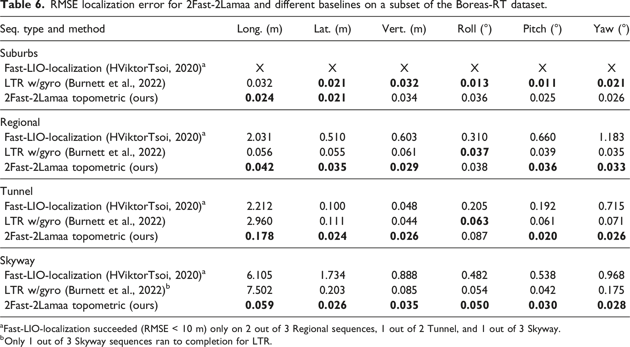
aFast-LIO-localization succeeded (RMSE < 10 m) only on 2 out of 3 Regional sequences, 1 out of 2 Tunnel, and 1 out of 3 Skyway.
bOnly 1 out of 3 Skyway sequences ran to completion for LTR.
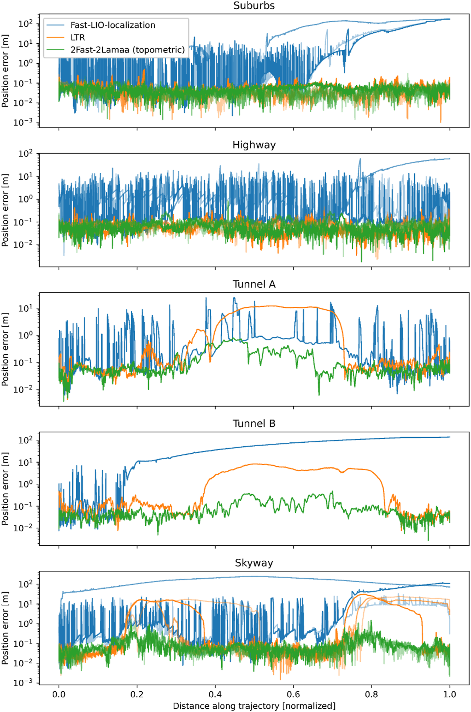
Localization error (position [m] with logarithmic scale) against travelled distance of 2Fast-2Lamaa and the different baselines on the Boreas-RT dataset. The different sequences are shown with different shades of colour.
We also want to remind the reader that the Regional sequences are run in both directions for localization, while the mapping is done only in one, as previously illustrated in Figure 12. When considering the sequence where the car is travelling in the same direction as the mapping run, the RMSEs are: Long. = 0.030 m, Lat. = 0.025 m, Vert. = 0.029 m, Roll = 0.029°, Pitch = 0.022°, and Yaw = 0.028°. These values are similar to those obtained in the easiest environment (Suburbs), demonstrating robustness to high-velocity trajectories.
9.4. Newer College dataset
9.4.1. Dataset description
To demonstrate the versatility of 2Fast-2Lamaa, we benchmark it using a dataset collected with a handheld device, the Newer College Dataset (Ramezani et al., 2020). It consists of five sequences collected while walking around the New College at the University of Oxford (UK) with a sensor suite equipped with an Intel RealSense D435i stereo camera and an Ouster OS1-64 lidar. Both sensors possess an embedded IMU. In our experiments, we only use the lidar and its internal IMU. The dataset also provides a detailed map of the environment as a coloured point cloud acquired with a Leica BLK360 survey lidar. The ground-truth trajectory of the sensors is obtained by registering the individual lidar scans to the map with ICP.
9.4.2. Baselines and metrics
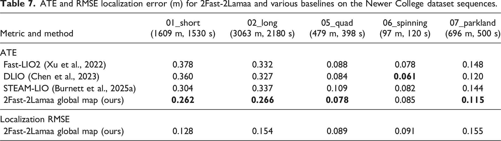
For odometry, we adopt the standard absolute trajectory error (ATE) to benchmark against various lidar-inertial frameworks. The ATE is defined as the RMSE between the positions of the estimated trajectory and the ones of the ground-truth after alignment using the Umeyama algorithm (Umeyama, 1991). Similarly to the evaluation with the Boreas-RT dataset, we use Fast-LIO2 (Xu et al., 2022) and STEAM-LIO (Burnett et al., 2025a) as baselines. We also include DLIO (Chen et al., 2023) as it is one of the best performing methods on the Newer College dataset.
It is important to note that the ground-truth provided in the Newer College dataset is not as accurate as that of the other datasets in our experiments. In their paper, Ramezani et al. (2020) showed that when the system is static at the start of the dataset, the ground-truth position jitters in a sphere of around 15 cm in diameter. Additionally, we empirically found a non-negligible rotational error (up to 2°) that hinders the use of the Boreas localization metric, thus preventing the evaluation of localization from one sequence to the other. 4 Accordingly, we only perform localization against the provided map with 2Fast-2Lamaa as a demonstration of its ability to perform localization within an existing global map. We compute the localization RMSE directly between the provided ground-truth positions and the estimated ones as a sanity check.
9.4.3. Odometry benchmark
ATE and RMSE localization error (m) for 2Fast-2Lamaa and various baselines on the Newer College dataset sequences.
9.4.4. Localization benchmark
The localization RMSE of 2Fast-2Lamaa is reported in the last line of Table 7. As mentioned previously, the ground-truth accuracy level does not allow for a thorough analysis of the proposed pipeline’s localization performance. Accordingly, it is difficult to draw any conclusion from these figures. However, these results demonstrate the soundness of the proposed approach and its ability to perform localization in a map generated with another sensor and mapping algorithm.
9.5. VBR-SLAM dataset
9.5.1. Dataset description
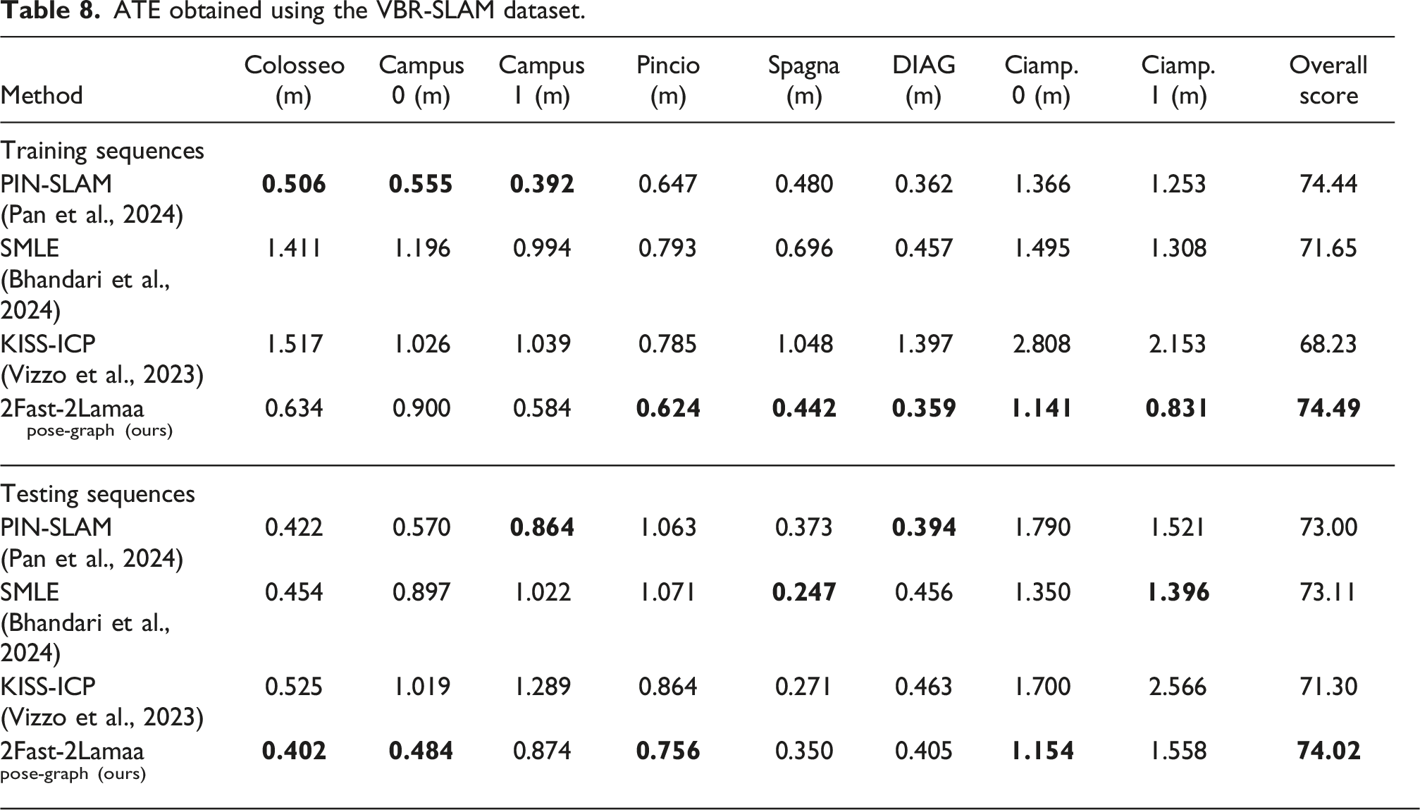
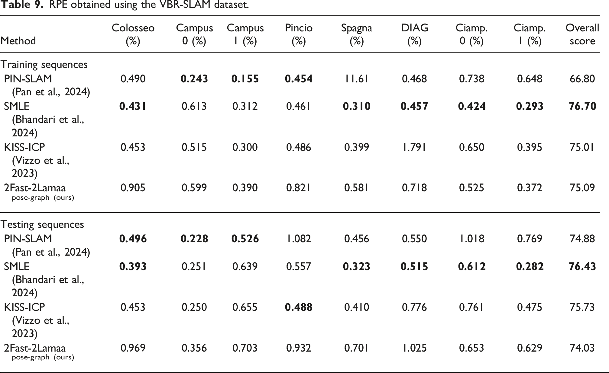
To further demonstrate the versatility of 2Fast-2Lamaa and the proposed online loop-closure detection and correction mechanism, we benchmark our method on the VBR-SLAM dataset (Brizi et al., 2024). It consists of 16 sequences collected with a lidar, stereo vision, and an RTK-GPS-IMU solution in 6 different environments. Half of the sequences use an automotive platform with an Ouster OS0-64 lidar at 20 Hz (environments Campus and Ciampino). The other half is collected using a handheld sensor suite comprising an Ouster OS1-128 lidar, which collects scans at 10 Hz (environments Colosseo, Pincio, Spagna, and DIAG). In both scenarios, 2Fast-2Lamaa uses the lidar’s embedded IMU. Out of the 16 sequences, only 8 have publicly available ground-truth. The ground-truth of the other sequences is held out for use in the dataset’s public leaderboard. In this section, we only leverage sequences with provided ground-truth. 5
9.5.2. Baselines and metrics
As the trajectories form large loops, we use 2Fast-2Lamaa with the online loop-closure detection and correction mechanism from Section 7. We use PIN-SLAM (Pan et al., 2024), SMLE (Bhandari et al., 2024), and KISS-ICP (Vizzo et al., 2023) as lidar-based baselines. PIN-SLAM is especially designed for state estimation with loop closures. As done in the VBR-SLAM public benchmark, we report both the RMSE ATE, and the relative pose error (RPE) as computed with the VBR-provided script. The RPE corresponds to the KITTI odometry metric, but computed with trajectory chunks of different sizes proportional to the whole trajectory length. The VBR-SLAM dataset also provides an overall score that aggregates the results throughout all the sequences to rank the different methods (the higher the better).
9.5.3. SLAM benchmark
ATE obtained using the VBR-SLAM dataset.
9.5.4. Odometry benchmark
RPE obtained using the VBR-SLAM dataset.
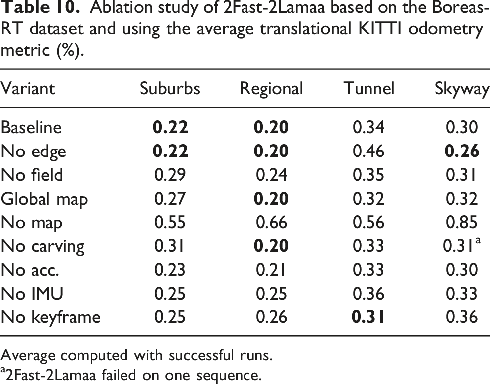
9.6. Ablation study
Ablation study of 2Fast-2Lamaa based on the Boreas-RT dataset and using the average translational KITTI odometry metric (%).
Average computed with successful runs.
a2Fast-2Lamaa failed on one sequence.
Ablation study of 2Fast-2Lamaa based on the Boreas-RT dataset and using the RMSE position error (m).
9.6.1. Features
2Fast-2Lamaa’s undistortion modules extract planar and edge features from the raw data, and these are used for point-to-plane and point-to-line distance residuals in the optimization. As a reminder, the first type is obtained by simply subsampling the incoming data, while the second corresponds to jumps in range. As per the discrete nature of lidar data collection, limited by a certain angular resolution, the likelihood of acquiring a point exactly on the edge of an object in the real world is null. On the other hand, a point that belongs to a plane in the real world is not affected by the sensor resolution: multiple consecutive points are likely to belong to the same planar patch (given that the observed plane is large enough). Thus, when considering the reality of lidar data collection and the downstream distance-based residuals, edge features create noisier constraints in the optimization process. However, they provide more constraints due to a single DoF, where planar residuals have two. In environments that are rich with structural elements, we expect the use of both feature types to perform similarly or worse than using solely planar points. Inversely, edge features provide crucial complementary information in geometrically challenging environments such as tunnels, where planes alone do not constrain the longitudinal motion. This reasoning is empirically verified in Table 10 with the No edge variant that performs better than the baseline for Skyway and significantly worse on Tunnel sequences. Note that even without the edge features on these sequences, 2Fast-2Lamaa still outperforms the methods benchmarked in Table 5.
9.6.2. Continuous distance field
In this paragraph, we discuss the contribution of the continuous distance field map towards the global performance of the framework. 2Fast-2Lamaa allows for the direct use of point-to-point distances with the centroids of
9.6.3. Global map versus submaps
As discussed in Appendix A.3, the use of i-Octree enables fast distance queries in incrementally built large-scale maps. If the system’s trajectory does not form large loops that accumulate too much drift, using a single map (as opposed to a succession of submaps) enables the estimation of globally consistent trajectories and maps. If the system’s trajectory does not form large loops, the drift of the estimated state when revisiting previously mapped locations might be small enough to enable the use of a single global map instead of a succession of submaps. Figure 14 illustrates the trajectory obtained when using an incrementally built global map on a Suburbs sequence. Note that 2Fast-2Lamaa is the only method that can provide a consistent trajectory (and map) as the other frameworks end up ‘forgetting’ previously traversed areas. Looking at the odometry metrics for Global map in Table 10, ‘single-way’ routes (Regional and Tunnel) are not affected by the change from submap to global map for scan-to-map registration, as expected. Interestingly, the routes that loop before heading back to the starting position are impacted negatively. This is due to the high sensitivity of the KITTI odometry metric to the orientation estimates. When the trajectory revisits a previously mapped area, due to some drift, the current state estimate can deviate from the locally consistent odometry to align the current data to the ‘old part’ of the map. This creates small ‘jumps’ in the trajectory estimate. As the KITTI odometry errors are computed after aligning a single pose per trajectory chunk, this deviation, especially in orientation due to a significant lever arm effect for trajectory chunks from 100 to 800 m, locally degrades the metrics. Estimated trajectories with 2Fast-2Lamaa and the different baselines on a Suburbs sequence. 2Fast-2Lamaa, with an incrementally built global map, is the only method that produces a trajectory that ends at the same location as the ground-truth. Note that none of the frameworks perform explicit loop-closure correction.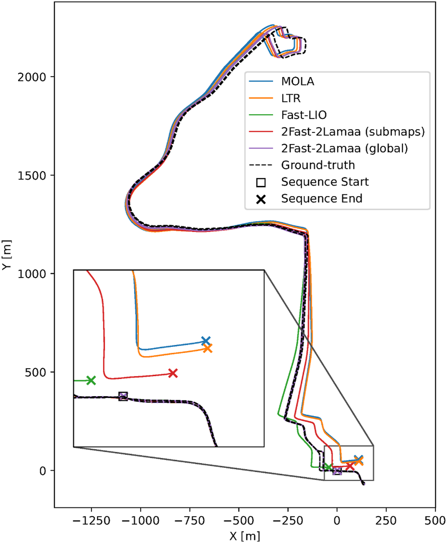
This last phenomenon does not really impact the localization performance within the global map in well-structured environments. As shown in Table 11, the results do not significantly change between the baseline and the Global map variant except for the Tunnel and Skyway sequences. We believe that the inherent drift of 2Fast-2Lamaa when building the global map hinders the sharpness of the few features present in the Tunnel and sequences (mostly corresponding to sparse service doors). Having ‘blurred’ features in the map prevents high accuracy along the longitudinal axis. For the Skyway sequences, the vertical axis is significantly impacted, while the lateral error is slightly higher. This is due to the drift of the mapping trajectory creating ‘double grounds and walls’ in areas of the map. Note that the estimated pose errors stay similar for the other axes. While not really demonstrated here, an advantage of building globally consistent maps for later localization is the simplicity of the localization process. For 2Fast-2Lamaa, it is a simple scan-to-map registration. There is no need for a complex module to perform topometric graph navigation.
9.6.4. Map cleaning
Another component of our ablation study concerns the removal of dynamic objects from the submaps when performing odometry and localization. For odometry, the baseline includes an online free-space carving mechanism. The No carving variant does not possess this feature. The results in Table 10 show no difference on Regional and Tunnel, but the Suburbs and Skyway are negatively impacted, respectively, with a higher error and a failure case.
As mentioned in the methodology part of this paper, the free-space carving can also be performed offline, given the mapping trajectory estimate, the map(s), and the undistorted scans. The localization baseline leverages both online and offline free-space carving during the mapping stage. The Online-carved map variant refers to the use solely of the online carving, and the No carving one does not perform any dynamic object removal. Figure 15 illustrates the difference between the uncarved, online-carved, and offline-carved maps. Overall, the presence of dynamic points in the map does not seem to have a significant impact on localization on the Boreas-RT dataset. A deeper analysis of the impact of dynamic points for localization with more datasets and sensors is required before drawing any final conclusion. Illustration of the dynamic object removal results in a map slice from a Suburbs sequence. Most of the dynamic objects are removed by the online free-space carving process.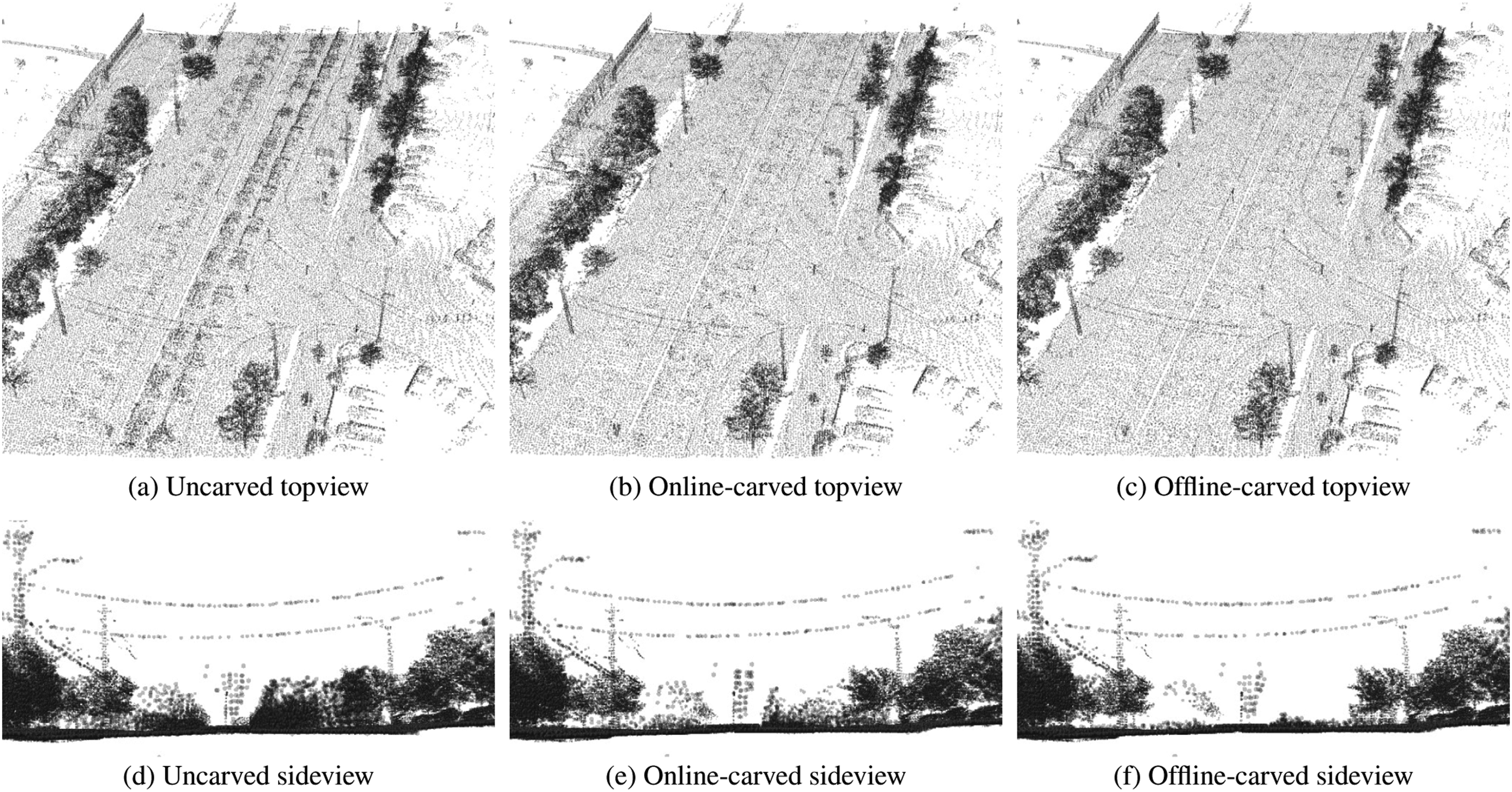
9.6.5. IMU versus constant velocity
2Fast-2Lamaa’s motion-distortion correction is based on continuous preintegration to characterize the trajectory of the system. This continuous state can be replaced with a strict motion model during the interval [τi-1, τi+1], similarly to MOLA. In this setup, we test two combinations of motion model: gyroscope preintegration with constant linear velocity (noted No acc.), and both linear and angular constant velocities (noted No IMU). The results in Table 10 show a drop in performance of both variants when compared to the baseline while still staying competitive. As expected, the performance of No acc. is better than that of No IMU. It is important to note that this analysis is based on automotive data. Thus, the movement of the platform is close to a constant velocity model. We expect a larger difference in performance with handheld or drone-mounted sensors.
9.6.6. Keyframing
To provide a deeper insight into our framework’s parameters, we evaluate the 2Fast-2Lamaa’s performance without keyframing and a lower number of points (2000) for scan-to-map registration, matching the parameters used on the VBR and Newer College datasets. This variant is denoted No keyframe in Table 10. Our method still outperforms state-of-the-art baselines from Table 5 on average. The total computational load is moderately impacted by this change of parameters, with 9.60 % total CPU load for the Baseline and 15.4 % for No keyframe.
9.7. Computational requirements
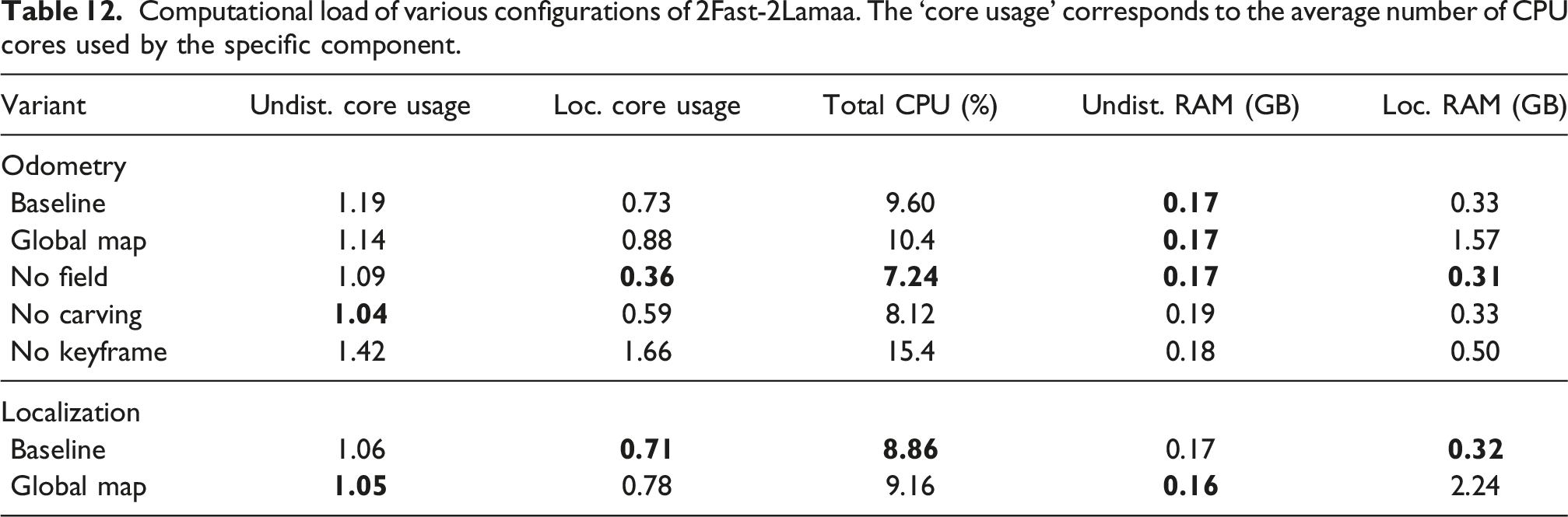
Computational load of various configurations of 2Fast-2Lamaa. The ‘core usage’ corresponds to the average number of CPU cores used by the specific component.
10. Conclusion
In this paper, we present 2Fast-2Lamaa, a lidar-inertial mapping and localization framework that consists of two main components: an optimization-based motion-distortion correction module and a scan-to-map localization algorithm that can build maps incrementally. Given sufficient geometric features in the lidar’s surroundings, the undistortion step estimates the continuous trajectory of the sensor through point-to-line and point-to-plane distance minimization between consecutive scans. The local trajectory is characterized by the inertial data directly through continuous IMU preintegration. Thus, the initial conditions (gravity direction, linear velocity, and biases) are the only state variables to estimate, making the problem efficient to solve. For motion consistency over longer horizons, the scan-to-map registration is performed using GP-based distance fields. Thanks to the use of efficient data structures and locally computed GPs, the scan alignment can be done in real time. In odometry/mapping mode, the map is incremented after every scan-to-map registration. An optional online loop-closure detection and correction step, based on a pose-graph optimization, gives 2Fast-2Lamaa the ability to estimate globally consistent trajectories if required.
Throughout an extensive experimental analysis using data from automotive and handheld platforms, 2Fast-2Lamaa demonstrates state-of-the-art accuracy for odometry, localization, and SLAM. Results were consistent across the different test environments, even with challenging routes going through feature-limited tunnels where baselines’ performance significantly declined. Note that these environments are not fully feature-deprived, as regular features such as service doors are present along the traffic lane. To address fully feature-deprived scenarios, our future work includes three different directions that are: the integration of intensity information in both the undistortion and localization modules, the fusion with vision sensing, and the exploration of Doppler velocity measurement with frequency modulated continuous wave (FMCW) lidars.
Footnotes
Funding
The authors received no financial support for the research, authorship, and/or publication of this article.
Declaration of conflicting interests
The authors declared no potential conflicts of interest with respect to the research, authorship, and/or publication of this article.