
Abstract
Unmanned underwater vehicles (UUVs) have been deployed for fish net-pen visual inspection (FNVI) in offshore aquaculture. Limited energy capacity of onboard power supplies constrains the UUV’s working range and operating time. To minimize the energy consumption by the UUV during the FNVI of the Blue Endeavour Project (an offshore salmon farm of the New Zealand King Salmon Company), an energy-optimal linear quadratic tracking (EO-LQT) control scheme is proposed in this paper. For EO-LQTs implementation, a new Linear-Parameter-Varying (LPV) system that approximates the nonlinear UUV dynamics model with an accuracy of approximately 99% regardless of the operating points in real-time, with the modified versions of Bhāskara I’s sine approximation and Shirali’s cosine approximation, is developed. The use of the Lagrangian under the Principle of Least Action with the UUV’s kinetic energy and the non-quadratic thruster power function in the EO-LQT performance index (PI) is demonstrated. The steps to solve the Hamilton-Jacobi-Bellman (HJB) equation with the non-quadratic Hamiltonian
Keywords
1. Introduction
In fulfilling the market demand for production, traditional inshore or nearshore aquaculture is facing the shortage of a suitable aquaculture environment for species such as King Salmon which requires cooler water temperatures (e.g., 12°C − 16°C) and adequate water flow, catering a natural environment for ideal fish growth (Preece, 2021). Other challenges of the existing aquaculture inshore or nearshore are environmental impact and conflicting coastal usages such as tourism, recreation, and conservation (Chu et al., 2020). As the inshore and nearshore areas reach the social carrying capacity, the New Zealand Government Aquaculture Strategy specifically mentions that by expanding into the open ocean, aquaculture presents transformational opportunities for its $3 billion industry by 2035, together with sustainable land-based farming (The New Zealand Government (Accessed 29 February 2024)). However, offshore aquaculture requires technical advancements for the farm and the workforce to withstand the harsh working environment. To minimize the safety concerns of the workforce and high operating costs in the long term, unmanned underwater vehicle (UUV) deployments are being reported mostly for remote operations in the industry and for autonomous operations in research and development (Amundsen et al., 2021). One of the most common use cases of UUVs is to perform a fish net-pen visual inspection (FNVI) (Akram et al., 2022; Liao et al., 2022). For instance, the New Zealand King Salmon (NZKS) company deploys a remotely operated underwater vehicle (ROV), a type of UUV 1 , to perform fish net-pen cleaning and visual inspection (1) to prevent net-occlusion and (2) to identify fish net-pen holes, respectively.
The NZKS has a dedicated deployment team that routinely conducts fish net-pen cleaning and visual inspection tasks in its fish farm. It takes approximately 2.5 hours to complete the task for a square net-pen: 30 m × 30 m × 15 m as shown in Figure 1. So, for offshore aquaculture with larger fish net-pen in harsh working environments, the visual inspection task will become a more hazardous, time-consuming, and costly process. As such, an option is to deploy autonomous UUVs to conduct fish net-pen visual inspection as a first step to solve the above problems facing the manual operations. Fish farm with square fish net-pens of the New Zealand King Salmon company in Nelson, New Zealand.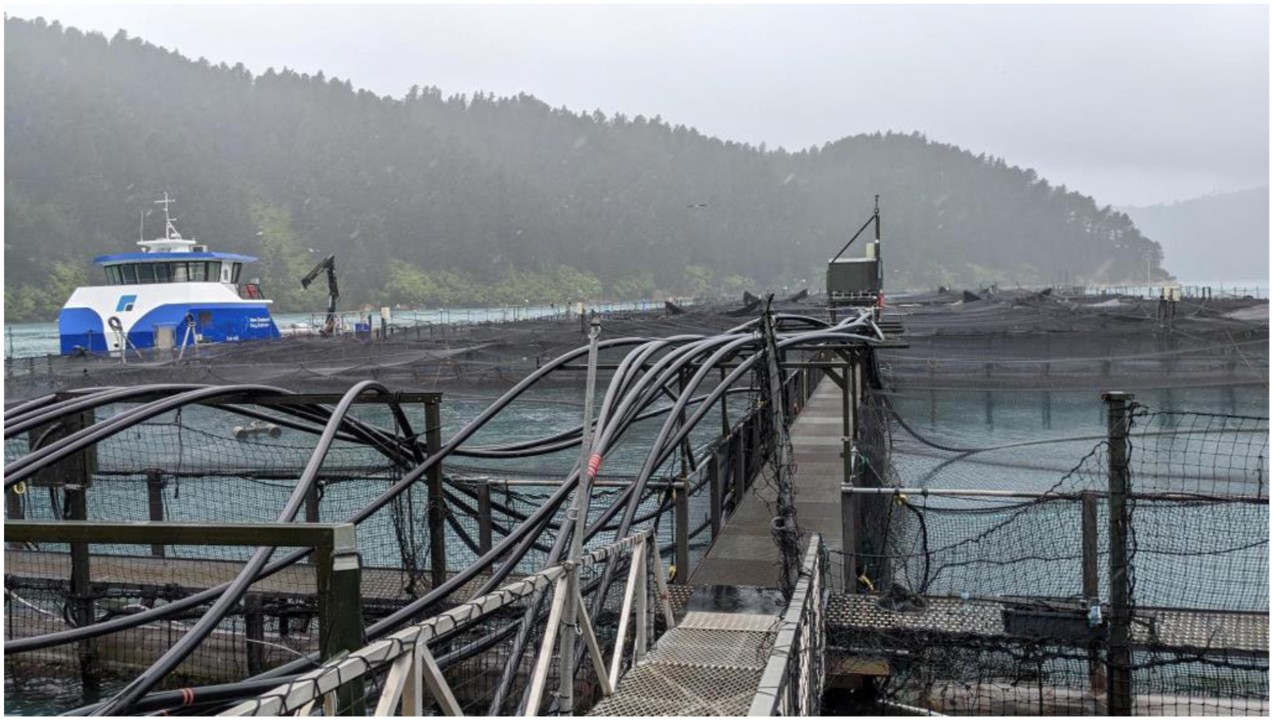
Unlike other torpedo-shaped UUVs in defense or oceanographic research, UUVs used for aquaculture are rectangular in shape, offering high maneuverability (with 6 or 8 thrusters) in a constrained environment. However, this type of UUV encounters more hydrodynamic effects such as added mass, damping, and other coupled nonlinear dynamic parameters (Kim et al., 2021). As a result, these increased hydrodynamic effects lead to higher energy demands for UUVs used in aquaculture applications. To solve this problem, the optimal design of a UUV with less hydrodynamic effects is proposed (Ao et al., 2024). However, due to the geometrical shape of the UUV and its effects on maneuverability as mentioned above, optimizing UUV shape alone will not resolve the task-specific requirements (e.g., the optimal slender body-shaped UUV cannot maneuver in the constrained operational environment of a fish farm.).
Alternatively, energy-optimality can be achieved at the UUV’s trajectory planning stage and real-time control stage with optimal control approaches. An online time-optimal trajectory planner for a slender body-shaped AUV called “nupiri muka” in a dynamic environment is reported in Lim et al. (2022). Energy-aware route optimization problem (EA-OP) is proposed and tested on an IVER3 AUV and a Nessie VII AUV in sea trials in De Carolis et al. (2018). Online Energy-Efficient Stochastic Trajectory Optimization (EESTO) using historical ocean currents data from Regional Ocean Modeling System (ROMS) is presented in Jones and Hollinger (2017). Another energy-optimal path planning with active flow perception of ocean current is proposed in Yang et al. (2021). Such planning approaches considering environmental disturbances are useful in oceanographic research covering a large range where the waypoints are not heavily constrained. In other words, there is a freedom to select the waypoints aligned with underwater current flow to minimize energy consumption. However, for FNVI operation, the waypoints (or areas of interest around the fish net-pen) are fixed. For the floating flexible cage system, the fish net-pen deforms due to the time-varying underwater current, but the visual inspection waypoints remain relatively the same around the fish net-pen. Therefore, the visual inspection trajectory usually covers areas where the underwater current might be against or aligned with. As a result, energy-optimal control, regardless of the trajectory planning, is more crucial for FNVI operation.
Energy-optimal depth tracking of an AUV using model predictive control (MPC) is proposed in Yao et al. (2019). Still, the proposed cost function or PI in the form of quadratic inputs (thrust) does not express power or energy explicitly and accurately according to either’s definition. Energy-optimal depth control using an infinite time linear quadratic regulator (LQR) on a linear time-invariant (LTI) model of an autonomous underwater glider (AUG), a special type of UUV, is proposed in Claus and Bachmayer (2016). Energy sub-optimal sliding mode control (SOSMC) is presented in Sarkar et al. (2016) in which the output from SMC is fed into finite-time LQR as the control input to be minimized. However, still, no specific power or energy function is used in the cost function. Using the thruster’s power function of DROP-Sphere AUV with 4 degrees of freedom (DoF), the development of a real-time energy-optimal MPC called RTEO-MPC, which can switch between solving static and dynamic surge motion optimizations, is proposed in Yang et al. (2018). The experiments of tracking two horizontal waypoints without obstacles or ocean currents are conducted using MATLAB/Simulink at the control loop rate of 10 Hz and a prediction horizon of 15 steps, and the results of RTEO-MPC are found close to that of the open-loop global optimal solution obtained from direct collocation (DC). Similarly, on the same platform, an energy-optimal economic MPC called EO-EMPC is developed considering the terminal cost (energy-to-go) in which static (surge and heave) and dynamic (surge, heave, and yaw) costs are considered (Yang et al., 2019). The results of EO-EMPC are compared to those of DC and line-of-sight MPC (LOS-MPC), achieving close performance to DC with substantially less computation time. In another work, the performances of conventional LOS-MPC (CLOS-MPC), nominal energy-optimal LOS-MPC (ELOS-MPC), ideal ELOS-MPC, and robust ELOS-MPC are compared in Yang et al. (2020), which reports that robust ELOS-MPC demonstrates higher energy efficiency, with reduced UUV travel time and lower root-mean-square error (RMSE), compared to other ELOS-MPC approaches. However, it is less efficient than CLOS-MPC in UUV traveling time and RMSE. In the controllers presented in the aforementioned literature, surge and yaw are controlled by MPC, and pitch and heave are controlled by proportional-integral-derivative (PID) control to reduce computational load. In Yang et al. (2024) for 3D path following under ocean currents, vertical setpoint (heave and pitch) tracking MPC and horizontal setpoint (yaw and surge) tracking MPC under 3D EO-MPC are proposed and compared with integral LOS-based control and 2D EO-MPC from Yang et al. (2020) and details of implementation of such decentralized MPC (DMPC) can be found in Shen et al. (2016); Shen and Shi (2020). This decoupled control approach is only suitable for the lawnmower-type operation with weak coupling between the vertical and horizontal planes of the system’s dynamics. It reports that, generally, at the expense of a substantial increase in UUV traveling time and a small variation in path-following error, 3D EO-MPC is more energy-efficient than others. An energy-optimal motion planning (trajectory generation and control) formulated as nonlinear robust MPC (NRMPC) and solved by an A∗-like algorithm is proposed in Huynh et al. (2015). Its energy function takes into consideration hotel load (used by computing and sensor systems without propulsion), energy to overcome inertia and drag forces, and estimated remaining energy for waypoints clearance. Energy-optimal motion planning for the Norwegian Experimental Remotely Operated Vehicle (NEROV) using direct shooting is proposed to solve the non-quadratic dissipated energy function of the thruster in Spangelo and Egeland (1992).
It is noted that in the above-mentioned literature relevant to UUV energy-optimal control, most of the UUVs are in slender-body/torpedo shapes, which suffer less from hydrodynamic effect than square/rectangular/box-shaped UUVs that encounter large hydrodynamic effect but offer high maneuverability. They also have large inertia to withstand high disturbances and have low DoF or are assumed to operate in a simplified scenario such as pure horizontal plane motion or depth control. They are not suitable for operation in constrained operational environments like fish farms. It is also noted that in the energy-optimal control schemes reported, most of them have no explicit power/energy functions used to define the cost functions. Additionally, they are not conducted in high-fidelity simulation environments with well-integrated hydrodynamic effects, which can be readily extended to field study. Alternatively, the literature on high-fidelity simulation does not necessarily cover the aspects of energy-optimality for use in offshore aquaculture. Moreover, numerical optimization-based control strategies (e.g., MPC) can handle the highly nonlinear and coupled UUV dynamics well but require high computing capacity. On the other hand, with a lower computation load, an analytical approach using a linear control strategy (e.g., conventional LQR or linear quadratic tracking) can only operate around the operating point at which it is linearized.
To address the issues identified above, the main contributions of this paper include: • Formulation of the fish net-pen visual inspection task as an energy-optimal finite-horizon constrained optimization problem, namely energy-optimal linear quadratic tracking (EO-LQT) control • New development on Bhāskara I’s sine approximation and Shirali’s cosine approximation to extend their respective original domain to the full range (−π to π) • New development of a Linear-Parameter-Varying (LPV) system to approximate the highly nonlinear and coupled UUV dynamics model with an accuracy of approximately 99 % regardless of the operating points in real-time by adopting the proposed modified versions of Bhāskara I’s sine approximation and Shirali’s cosine approximation • Use of the Lagrangian under the Principle of Least Action (PLA) with linear and rotational kinetic energy, transformed into error states, to be adopted in the EO-LQT controller’s performance index (PI) • Use of the non-quadratic power function of UUV’s thruster, partially reflecting the unmodeled energy consumption normally ignored in the energy-optimal control, in the EO-LQT controller’s PI • Derivation of the new analytical optimal control form by re-solving the HJB equation with non-quadratic Hamiltonian • High-fidelity simulations of the proposed LQT controllers (CO-LQT and EO-LQTs), in the existing Robot Operating System (ROS)-based high-fidelity simulation platform, integrated with Gazebo Physics Engine called UUV Simulator (Manhães et al., 2016 (Accessed 20 November 2023)) • Performance validation of the proposed LQT controllers under three different underwater current speeds (e.g., 0.0 m/s to 0.9 m/s) in high-fidelity simulations • Experiments of the proposed LQT controllers in the pool, along with their respective high-fidelity simulations in the pool environment • Use of T200 thruster power function, approximated by the 6th-order polynomial regression, to compare real-time energy consumption among controllers in both high-fidelity simulations and pool experiments • Use of the publicly available specifications and the constraints of the Blue Endeavour Project (the first of its kind in New Zealand) of the New Zealand King Salmon Company and the lightweight and highly maneuverable BlueROV2 Heavy Configuration in these simulations (The New Zealand King Salmon Company (Accessed 25 November 2023); BlueRobotics (Accessed 02 August 2023))
The remaining part of this paper is structured as follows. Section 2 presents UUV’s 6-DoF nonlinear model, its state-space representation (SSR), and the subsequent Linear-Parameter-Varying (LPV) model using the modified versions of Bhāskara I’s sine approximation and Shirali’s cosine approximation. Section 3 discusses the CO-LQT control problem. Section 4 covers the formulation of energy terms which are used in Section 5 that details the EO-LQT control problem. Section 6 describes the Hamilton-Jacobi-Bellman equation, the necessary and sufficient condition for optimality, and the detailed steps of finding the conventional optimal control and non-quadratic optimal control. Section 7 explains high-fidelity simulations and experiments, covering the experimental setup for vision-based state-estimation that is implemented using a Kalman Filter and is crucial to conducting experiments in the pool. Section 8 discusses the results of FNVI simulations, pool experiments, and simulations, in terms of trajectory tracking, pose tracking, and energy consumption. Section 9 suggests future work to address the factors that potentially cause the performance differences of the controller between pool experiments and simulations, and highlights future research direction, targeted to field trials. Section 10 concludes the summarized findings of this research work.
2. Dynamic model of 6-DoF UUV
2.1. Nonlinear model
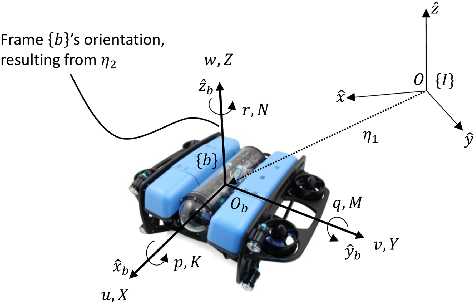
The 6-DoF nonlinear dynamic model consists of rigid body dynamics and the additional hydrodynamics due to the added mass, linear and quadratic damping (Antonelli, 2018; Fossen, 2011). The control wrench depends on the thrusters’ static configurations in the UUV frame {b}. The Society of Naval Architects and Marine Engineers (SNAME) nomenclature as shown in Figure 2 is used for the UUV’s dynamic modeling and the relevant reference frames are illustrated in Figure 3. SNAME nomenclature for the UUV’s dynamic modeling. BlueROV2 Heavy Configuration with SNAME nomenclature in East-North-Up (ENU) reference frame.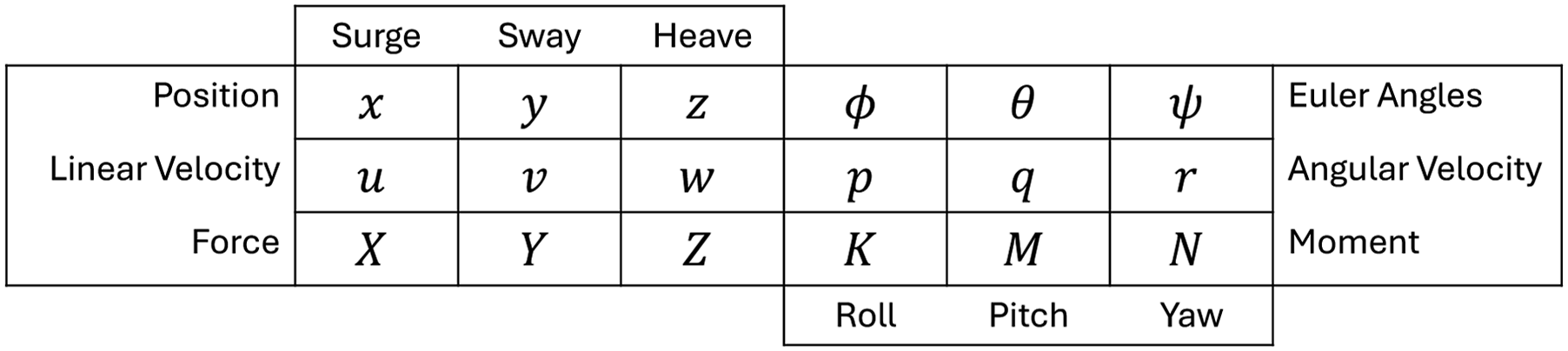
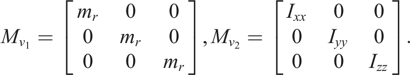
Assigning Frame {b} at the center of mass/gravity, the simplified mass matrix of the rigid body can be represented by
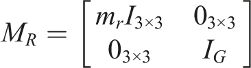
The UUV has three symmetric planes and is completely submerged in the water and operated at low speed during the operation.
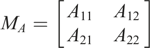
With Assumption 2.1, only the diagonal components of the mass matrix, contributed by the added mass, are taken into account,

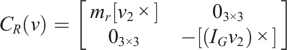
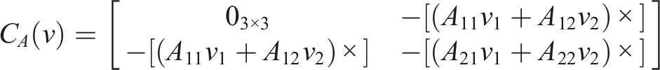
Using the added mass matrix, the Coriolis-Centripetal acceleration matrix, contributed by the added mass, can be described by
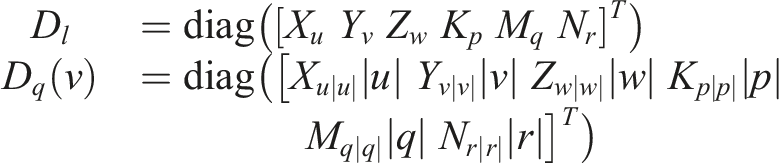
The approximated linear and quadratic damping matrices can be represented by
Suppose the jth thruster’s direction vector expressed in Frame {T
j
}, which is defined with respect to Frame {b}, is denoted by
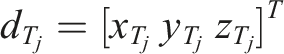
Then, with the thrust magnitude of fT,j, the jth thrust vector is
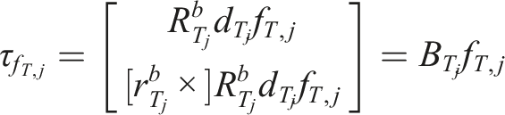
Therefore, the total wrench propagated by m number of thrusters can be described by

Using the terms mentioned above, the compact nonlinear dynamic model can be described in the form of

The UUV’s twist can be converted to the rates of change of position and Euler angles using the Jacobian

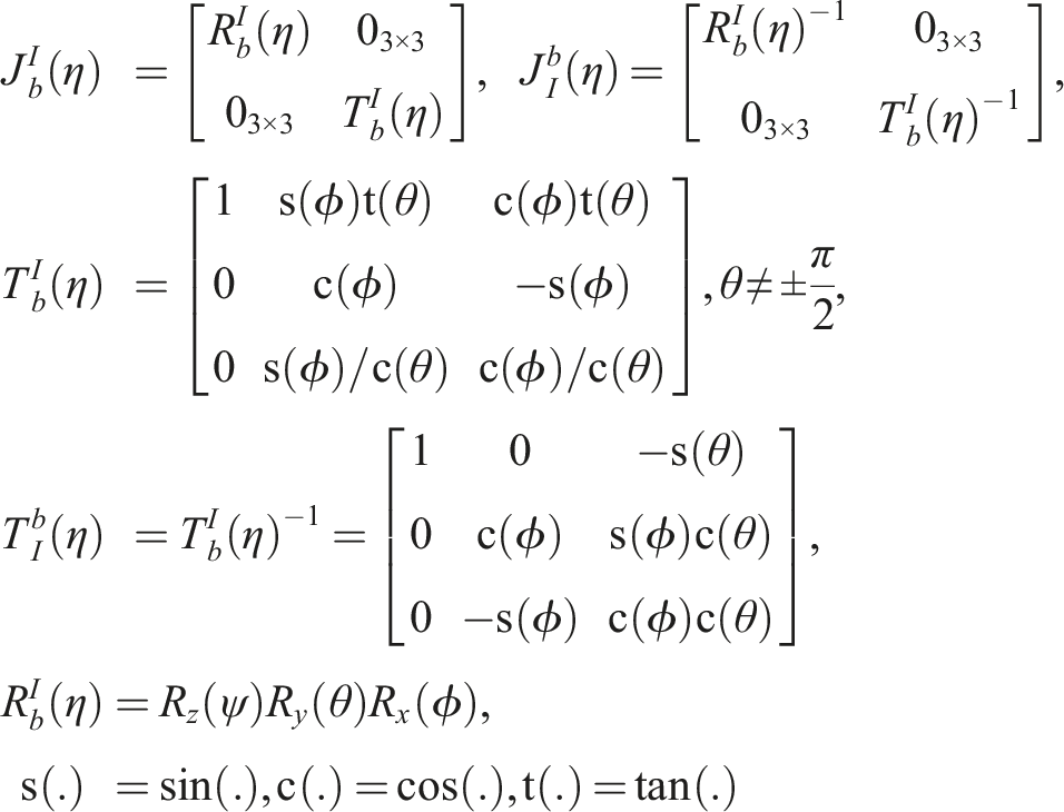
Let
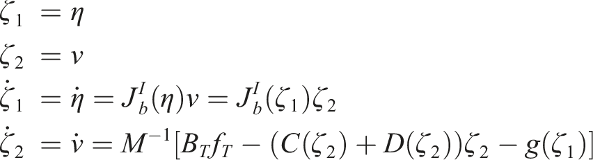
By rearranging the equations above, 12-state nonlinear state-space representation (SSR) model can be obtained as


To express all the states w.r.t Frame {b}, ζ1 and
In this work, the UUV’s 12-state nonlinear SSR model, represented by equations (4) and (6), will be used in the following subsection to develop the Linear-Parameter-Varying (LPV) system.
2.2. Linearized model
Conventionally, a nonlinear system is linearized to a Linear-Parameter-Varying (LPV) system via Jacobian at each operating point (MathWorks (Accessed 12 August 2023)). This method is based on the Taylor series expansion of the nonlinear system truncated at the first partial derivative around an operating point (ζ
o
, fT,o). For instance, equation (4) can be written as
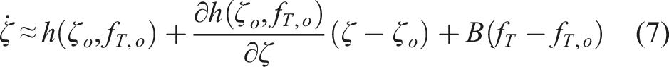
However, equation (7) is not suitable to produce a standard linear system (e.g.,
Suppose
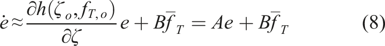
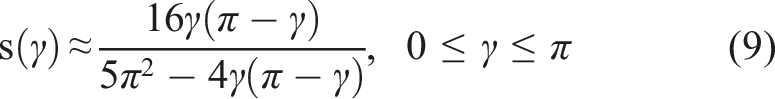
Therefore, instead of using the Jacobian method, the method of factorizing and extracting states ζ from equation (4) is proposed. In the term u|u|, u can be easily extracted, but this is not the case for sine or cosine functions. One way to deal with it is to represent sine (e.g., s(γ)) and cosine (e.g., c(β)) as rational functions such as Joseph (2009, p. 57) and Shirali (2011, p. 99),
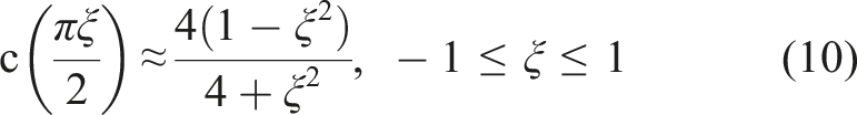
Letting
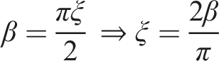
Equation (10) can be rewritten as
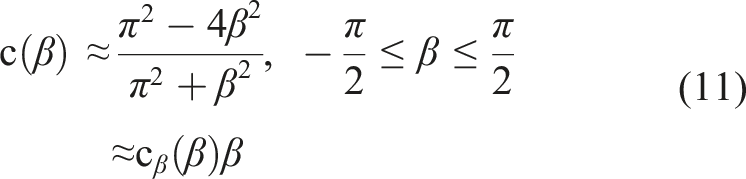
Equations (9) and (11) are modified further so that they can be factorized in a larger domain.

Using the properties of c
β
(β)2β2 + s
β
(β)2β2 ≈ 1, Sine approximation, resulting from the modified version (equation (12)) of Bhāskara I’s rational expression. Cosine approximation, resulting from the modified version (equation (13)) of Shirali’s rational expression.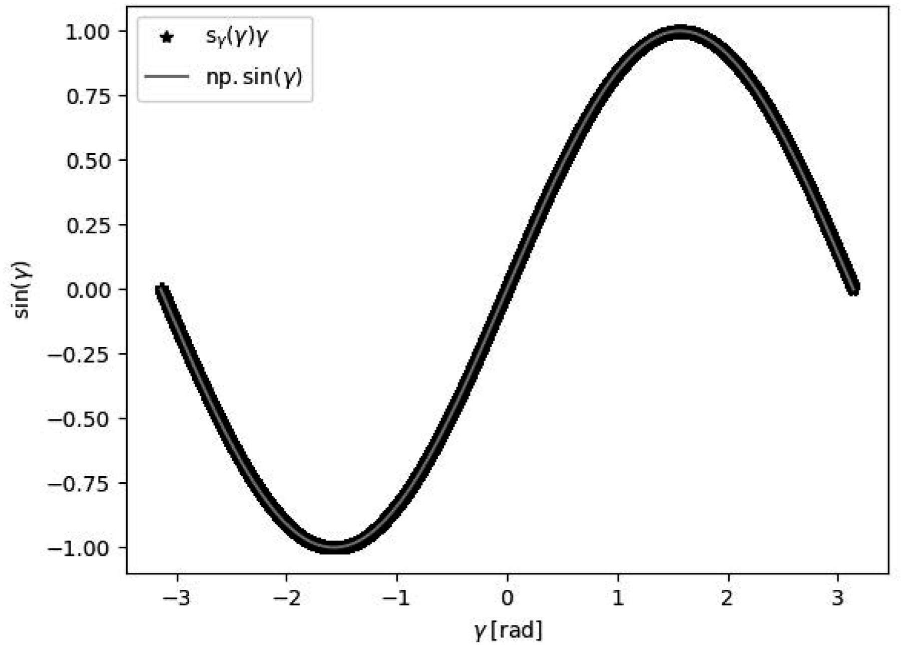
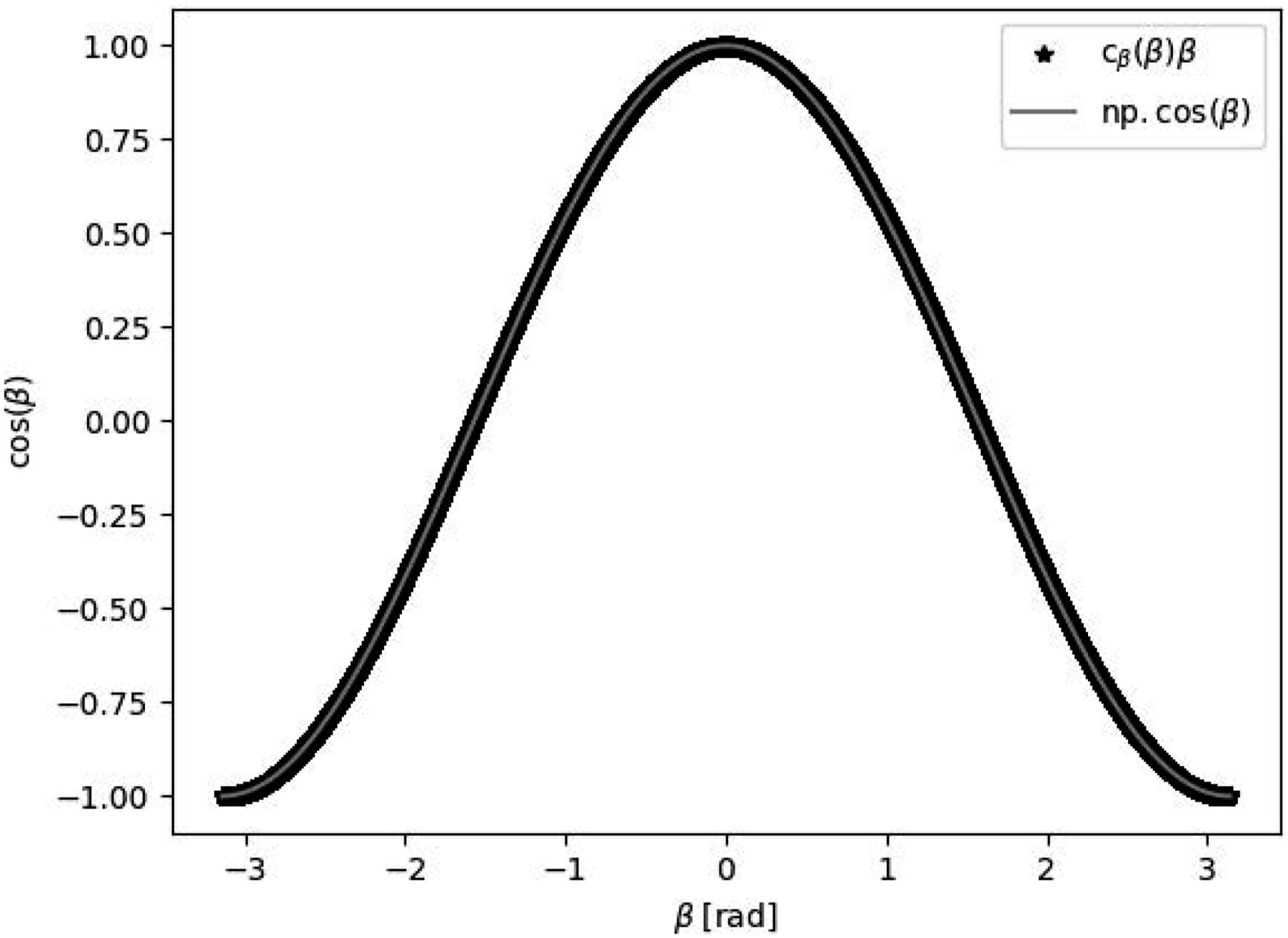

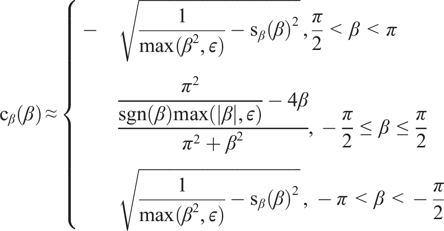
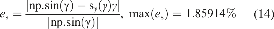
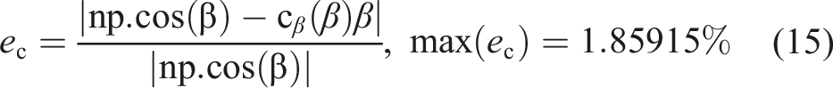
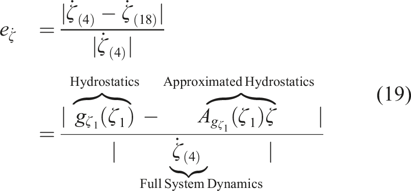
Therefore, our proposed method produces the approximated sine and cosine functions over the full domain with an accuracy of approximately 98 %.
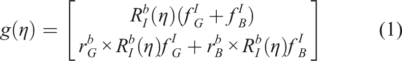
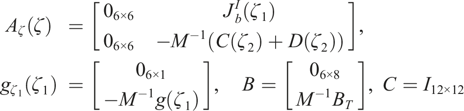
Using the techniques described above, equation (4) needs to be modified in the standard form for a Linear-Parameter-Varying (LPV) system. Firstly, due to the frame assignment of Frame {b} at the center of gravity, and the center of buoyancy in the positive z-axis (upward) of Frame {b}, the gravity vector and the buoyancy vector from equation (1) becomes
The simplified equation (1) becomes
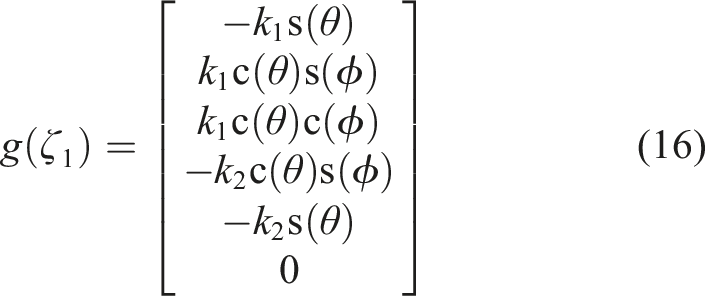
Subsequently, the proposed technique above for sine and cosine approximation will be applied on equation (16) such that it results in
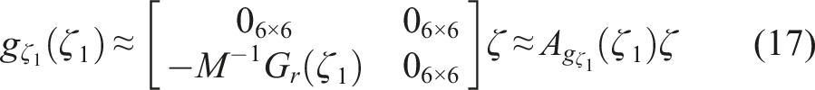
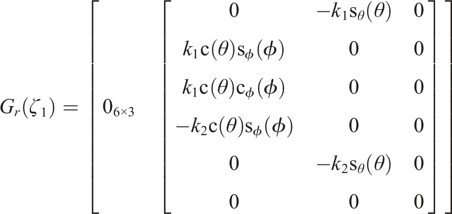
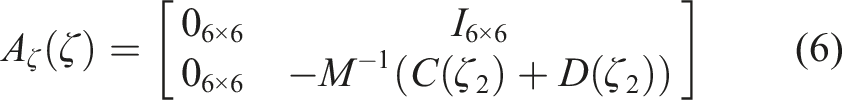
Finally, by substituting equation (17) into equation (4), the UUV’s LPV system can be described by

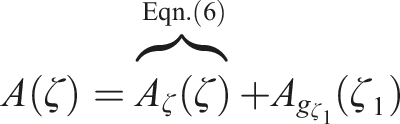
In a similar fashion to equations (14) and (15) for the elementwise comparison on equation (19),
The state-varying matrix A is also denoted as A(x, t), A(t), or A(x, k) (Morato et al., 2020).
3. Linear quadratic tracking control problem
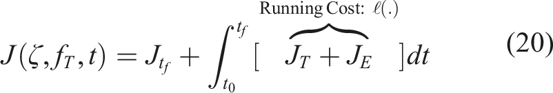
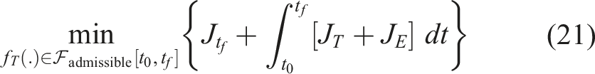
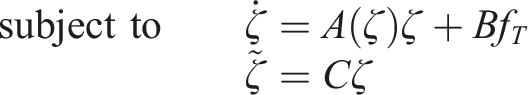
A general trajectory tracking problem in the sense of LQT is illustrated in Figure 6. In a generic LQT control for the fish net-pen visual inspection task, the performance index (PI) will be formulated as the finite-horizon Bolza type which includes both terminal cost and integral tracking cost, as shown in equation (20).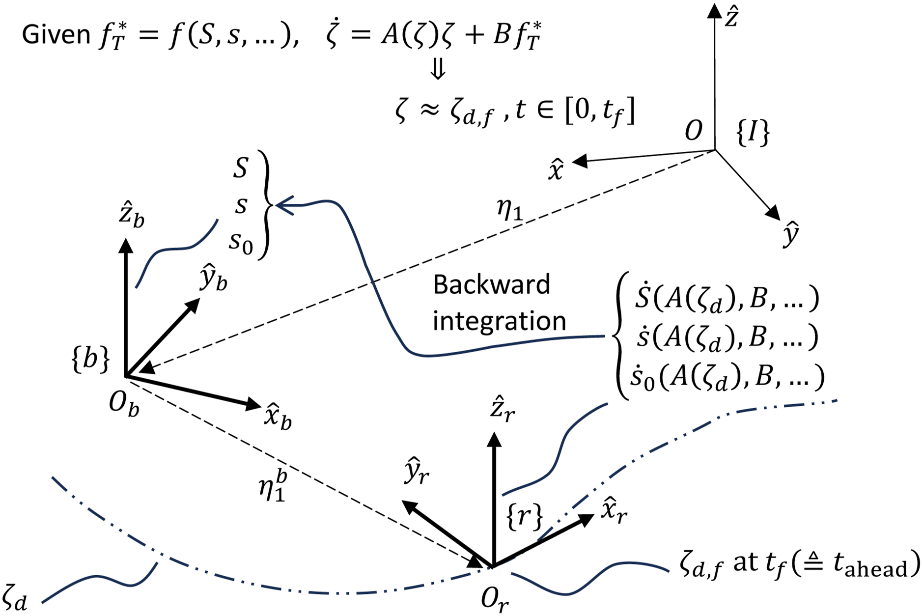
Therefore, the minimum cost function J^∗(ζ, t) is
4. Formulation of energy terms in the PI
The energy terms in the PI need to be established first before an EO-LQT controller can be designed. As shown in the UUV system’s dynamic model in equation (2), there are UUV’s states and inputs which are directly linked to the total energy consumption. According to the law of conservation of energy,

4.1. Energy associated with the UUV’s motion: Em
Generally, the energy associated with the UUV’s motion E
m
is related to the kinetic energy E
k
and the potential energy E
p
. Therefore, if these energy terms are embedded into the PI as a part of J
E
as shown in equation (21), the integration of the change in energy will result in action according to the Principle of Least Action (PLA), which states that the true trajectory is the one that results in the minimum action value of equation (24). Its use in optimal trajectory planning is demonstrated in Huang et al. (2023).
However, as mentioned in Remark 4.1, the potential energy: E
p
will not be considered. Therefore, equation (24) can be reflected in equation (21) as part of the energy-related term as shown below.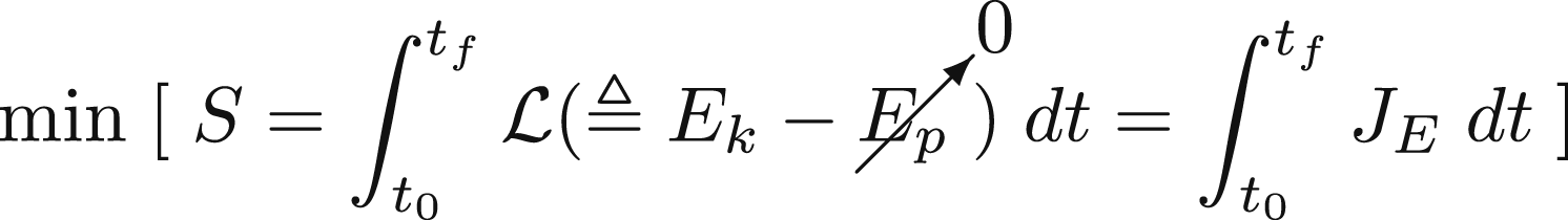
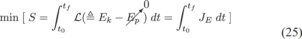
As the UUV can be configured mechanically to become neutrally buoyant, the potential energy resulting from the gravitational acceleration can be neglected. Although there are other types of potential energy (e.g., fluid memory effects), resulting from the environments and disturbances, they are not considered, as, unlike an unmanned surface vehicle (USV), the UUV will be fully submerged and will not operate at the free surface most of the time.
As
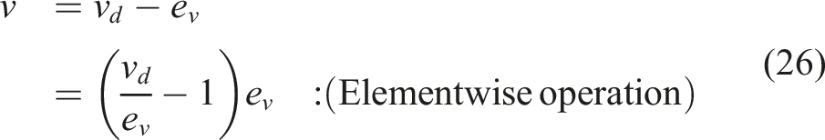
Subsequently, equation (26) can be rewritten, as a function of the full-state tracking error

Using equation (27), the kinetic energy can be expressed as follows:
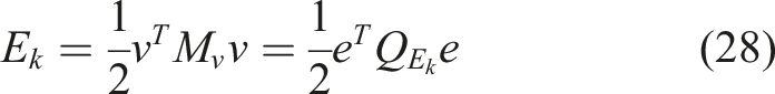
As E
k
consists only of ν as shown in equation (28), in the compatible form of LQT’s PI (either in state or control-effort), it now becomes a part of J
T
in equation (21) instead of J
E
. However,
4.2. Energy from the UUV thrusters
To determine the energy consumed by thrusters:


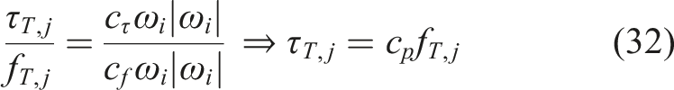
Therefore, the mechanical power of the jth thruster can be represented by

To write the power as a function of fT,j, the following relationship between τT,j and fT,j can be established.

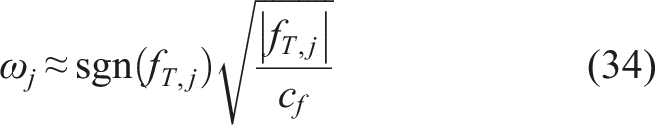
If ω
j
is not directly available from the thruster, it can be approximated as shown in equation (34) based on equation (30) as fT,j is available from the LQT controller output in real-time.
After establishing the individual thrusters’ power term as a function of ω
j
and fT,j, the total power term and quadratic power term of all thrusters as a function of f
T
can be written as follows:


The approximated linear relationship described by equation (33) can be observed in Figure 7. The least square linear regression estimates c
p
= 0.022 with R2 score (coefficient of determination) of 0.96 and thus, the regression model fits the data well. Mapping of ω
j
fT,j to pT,j of the jth T200 thruster.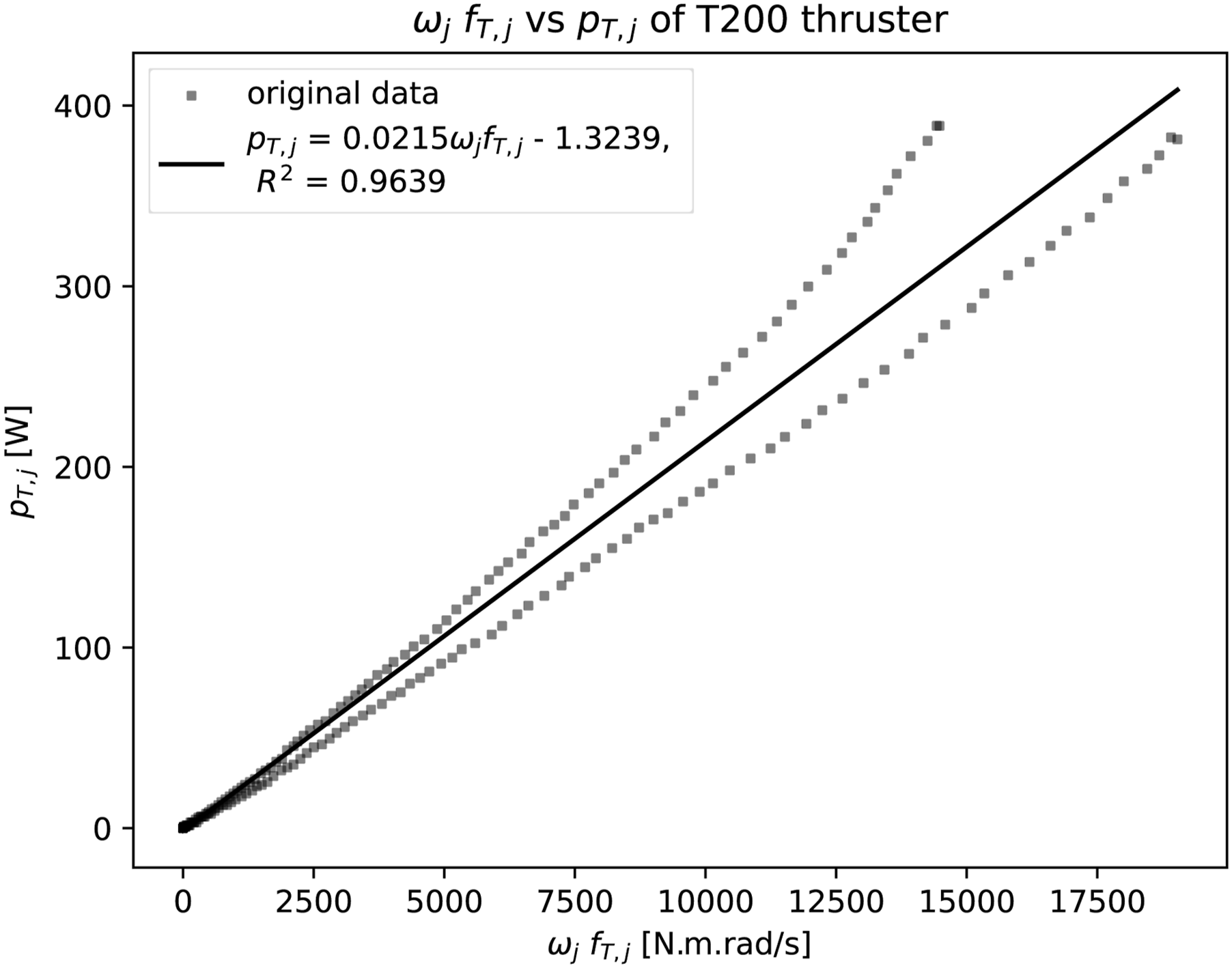
To improve the accuracy of the estimation of the energy consumption across various controllers during the analysis of experimental results, a higher-order polynomial function can be used to predict the power consumption pT,j of the jth thruster.
Therefore, using the publicly available dataset of T200 thruster, operating at 16 V, the polynomial regression on the relationship between thrust (N) and Power (W) will be generated, mapping fT,j to pT,j (T200 Thruster (Accessed 3 November 2023)). As shown in Figure 8, the resulting 6th-order polynomial regression yields, with R2 score of 0.99, in the form of Mapping of fT,j to pT,j of the jth T200 thruster. 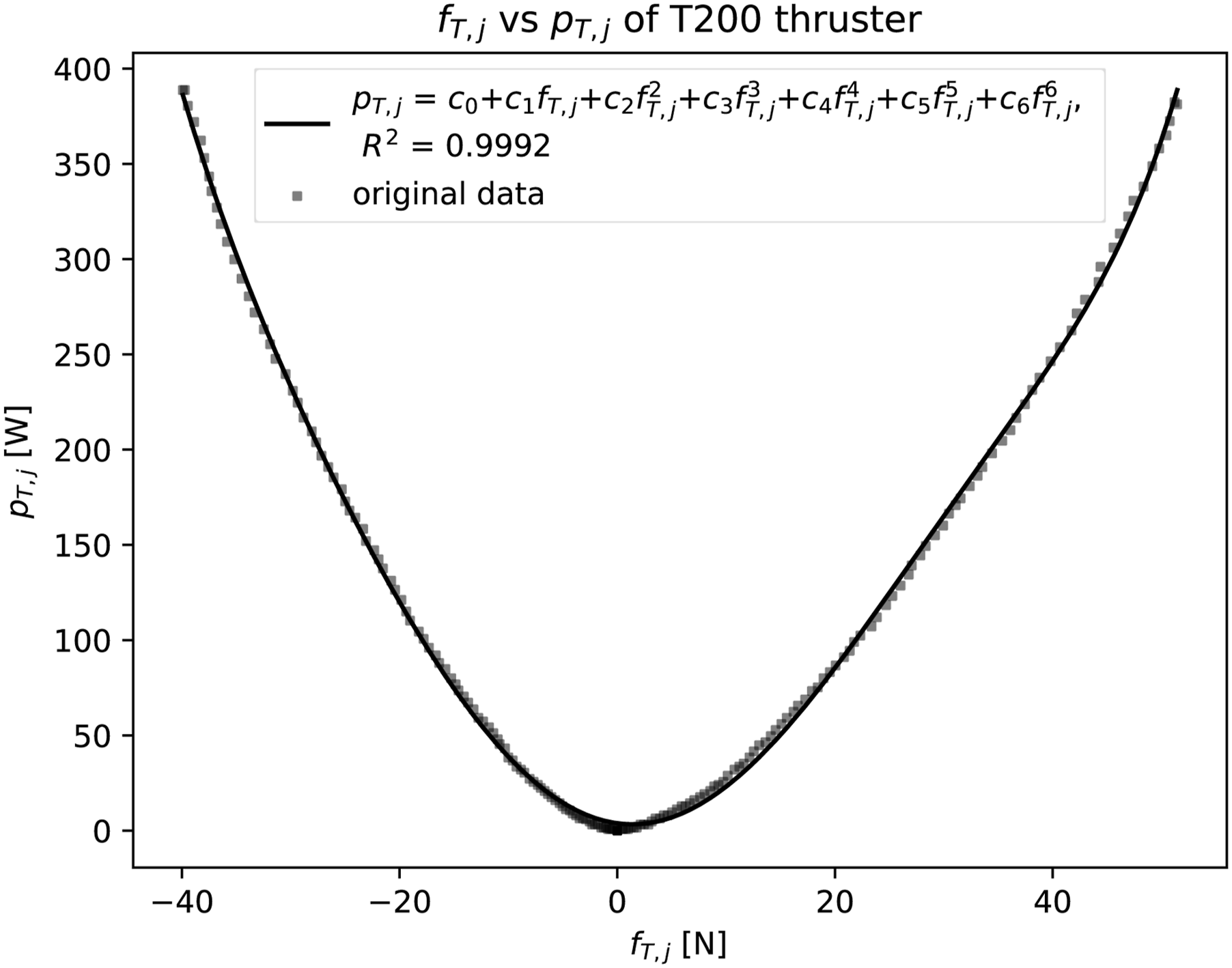
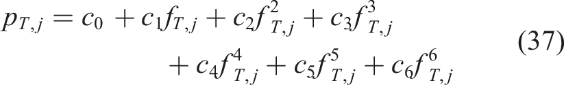
The total energy consumption of the thrusters at each control loop which is running with the control loop duration Δt is calculated using equation (37) as follows:
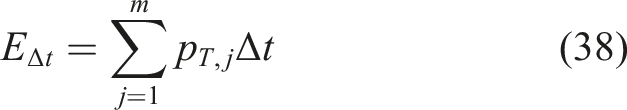
In the following section, E
m
(Specifically E
k
) in terms of tracking error states e and
Although E
h
is not dealt with directly in equation (21), it is part of equation (23). As such, the inclusion of E
m
and
5. Energy-optimal linear quadratic tracking control
Conventionally, J
T
and J
E
of CO-LQT control as shown in equation (21) are in quadratic form. Therefore, with the energy terms formulated above, the PI for EO-LQT control in quadratic form using E
k
as shown in equation (28) and quadratic power term of all thrusters as shown in equation (36) can be defined.
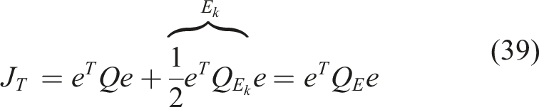
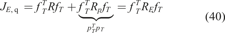
When using the total power term of all thrusters as shown in equation (35), there will be non-quadratic term involved as follows:

In JE,nq, the summation of
After formulating the relevant tracking cost J
T
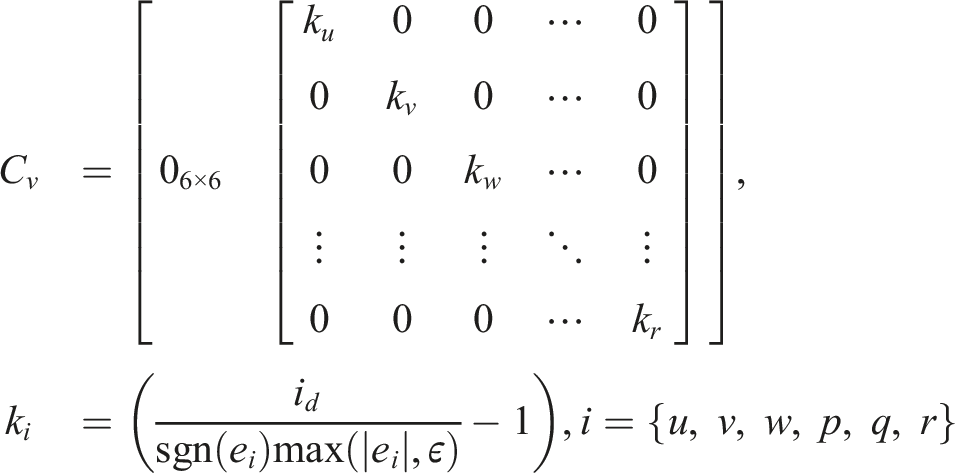
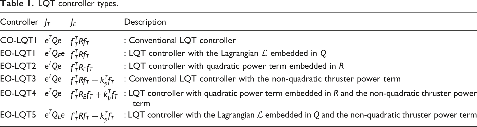
and energy costs JE,q, JE,nq for the EO-LQT control, the following six controllers with different PIs will be proposed to test the efficacy of those costs individually and in different combinations. The first controller is the conventional LQT controller, named CO-LQT1, which is exactly the same as equation (21) and will be used as a baseline controller for the comparison.
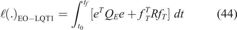
The second controller, named EO-LQT1, is designed from the tracking cost as shown in equation (39) which utilizes the Lagrangian
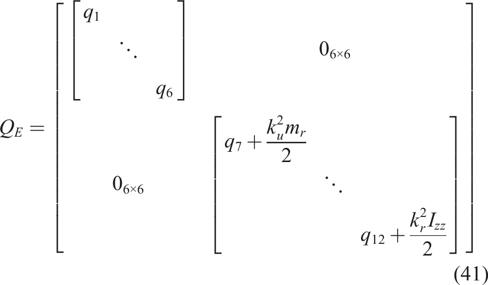
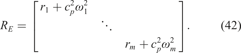
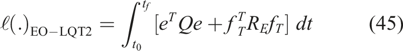
The third controller, named EO-LQT2, is formulated with the standard constant tracking penalty weight Q and the energy penalty weight with quadratic power term as shown in equation (40). Due to the auto-adjusted R
E
, this controller is expected to save energy consumption substantially.
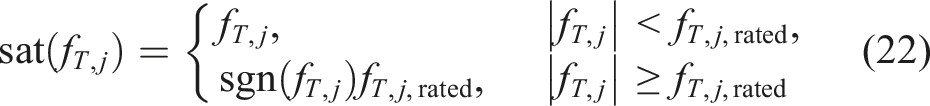
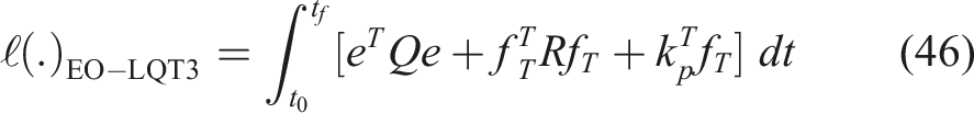
In the fourth controller, named EO-LQT3, the standard constant weight Q and R and the total power term in non-quadratic form as shown in equation (43) are used. As this controller involves non-quadratic term, the standard LQT equations cannot be used to find the energy-optimal control and thus, the detailed derivation will be presented in the next section.
The fifth controller, named EO-LQT4, is the combination of EO-LQT2 and EO-LQT3. This controller is designed with the standard constant tracking penalty weight Q and the quadratic and non-quadratic power terms. It is also expected to minimize energy consumption with a similar performance as EO-LQT3.
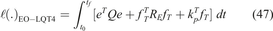
While energy-optimality is an important consideration, achieving a proper fish net-pen visual inspection requires a balanced trade-off between energy-optimality and trajectory tracking. The quadratic power term in EO-LQT2 and EO-LQT4 is expected to minimize energy consumption substantially and, at the same time, to have relatively larger tracking errors. However, another combination of the Lagrangian

As mentioned above, the six controllers are proposed with the minimally possible combinations of the formulated energy/power terms to investigate the trajectory tracking and energy-optimality performance.
LQT controller types.
6. Hamilton-Jacobi-Bellman equation: Necessary and sufficient condition for optimality
To obtain the optimal control, there exists a necessary and sufficient condition for optimality known as the Hamilton-Jacobi-Bellman (HJB) equation. As mentioned earlier, some of the proposed controllers have non-quadratic terms in PI and thus, there will be two separate derivations, one for purely quadratic PI and another for the PI with quadratic and non-quadratic terms.
6.1. Quadratic HJB and solution of the optimal control
Firstly, quadratic Hamiltonian 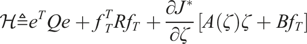
Therefore, the HJB equation based on 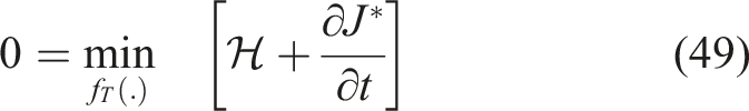
Unlike the infinite linear quadratic tracking problem, the optimal cost-to-go function J∗(ζ, t) consists of the state and time components (Tedrake, 2023). One possible definition for J∗(ζ, t) can be
Take the partial derivative of J∗(ζ, t) with respect to state ζ and time t, respectively.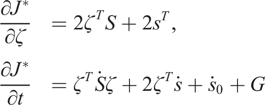

(Note: The term G is not considered in Tedrake (2023), and thus it is important to note that the resulting matrix differential equations are not the same. Especially, for the derivation based on the non-quadratic term, the matrix differential equations have additional terms.)
Setting the differentiation of equation (49) with respect to f
T
to be zero, we have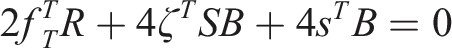
Therefore, the ideal optimal control without thrust saturation is

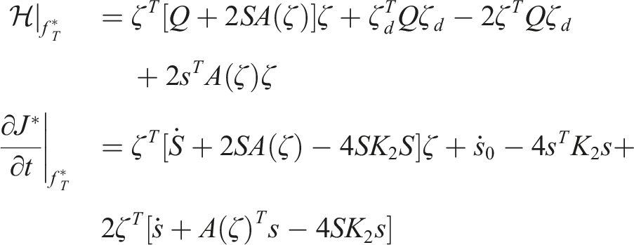
Hence, equation (49) becomes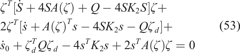
The resulting equation (53) implies that


Using the final conditions,


6.2. Non-quadratic HJB and solution of the optimal control
For the case of 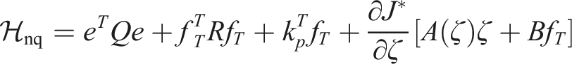
Therefore, the HJB equation based on 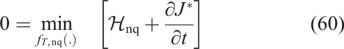
Following the same process for 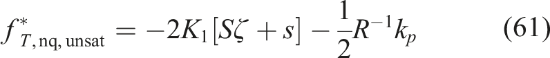

Substituting the optimal control expressed in equation (61) into the non-quadratic HJB as shown in equation (60), the resulting differential matrix and vector equations become


6.3. Uniform positiveness condition for J∗(ζ, t)
To ensure that J∗(ζ, t) is uniformly positive, the following conditions are needed (Tedrake, 2023).
Firstly, as shown in equation (50),
Secondly,
Although the resulting S and s ensure that Extracting the desired trajectory ζd,f at t
f
≜ t
ahead
. x
d
, y
d
, and z
d
are illustrated and so are other desired trajectory states with circular dots.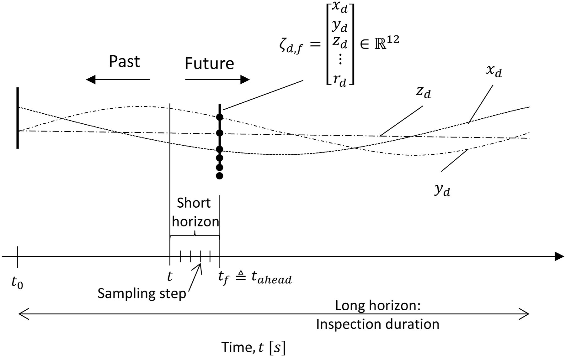
7. High-fidelity simulations and experiments
Number of simulations and experiments conducted.
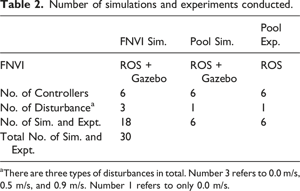
aThere are three types of disturbances in total. Number 3 refers to 0.0 m/s, 0.5 m/s, and 0.9 m/s. Number 1 refers to only 0.0 m/s.
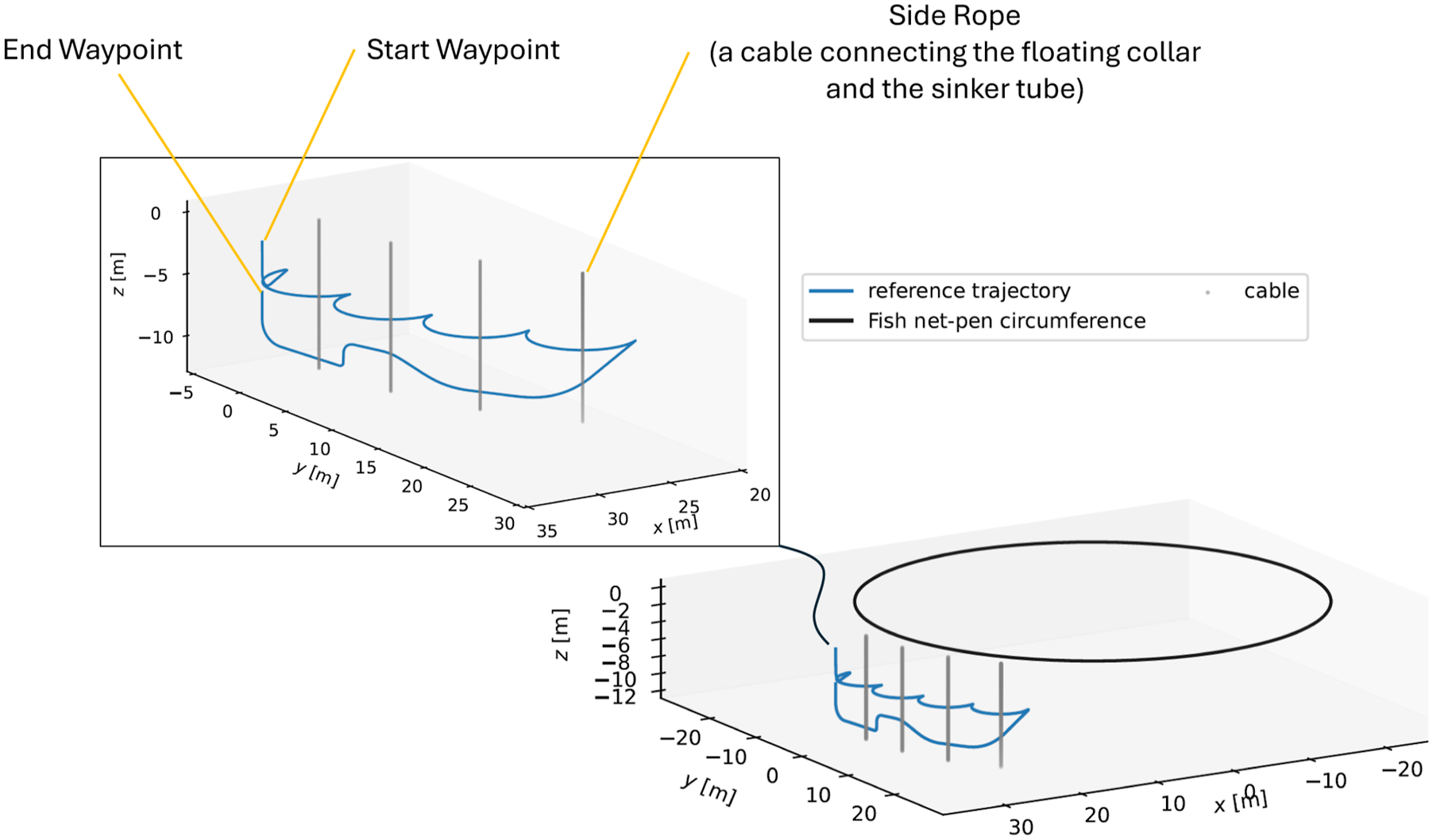
Illustration of the FNVI trajectory around the floating flexible fish net-pen from the operational perspective.
However, for the field trials in the open ocean, there are a few barriers (mainly budget constraint, expensive localization sensors, industrial-grade UUV, logistics and safety concerns) to deploying BlueROV2 Heavy Configuration in the actual fish farm at the current stage. Therefore, pool experiments are conducted, along with their respective simulations in ROS and Gazebo Physics Engine. Even in the case of pool experiments, the major challenge is the UUV localization, which will be detailed and addressed in the next subsection. As a result of this localization issue, a planar trajectory is utilized for the pool experiment; however, to consider realistic maneuvering capabilities required for the actual field trials in the future, the pool-experiment trajectory is designed with a sudden change in twist, curvature, and straight lines.
Hardware & Software specifications, controller tuning parameters, the numerical solvers for matrix differential equations, and ROS launch processes used in this work are summarized in Appendix A. The main difference between simulation and experiment is the availability of comprehensive state-estimation. In simulation, via Gazebo, the full state-estimation is readily accessible, whereas in experimental settings, the full state-estimation is one of the tedious tasks, and it can directly impact the performance of the controller and introduce confounding factors that compromise the experimental results. Therefore, the experimental setup for state-estimation will be detailed in the following subsection.
7.1. Experimental setup
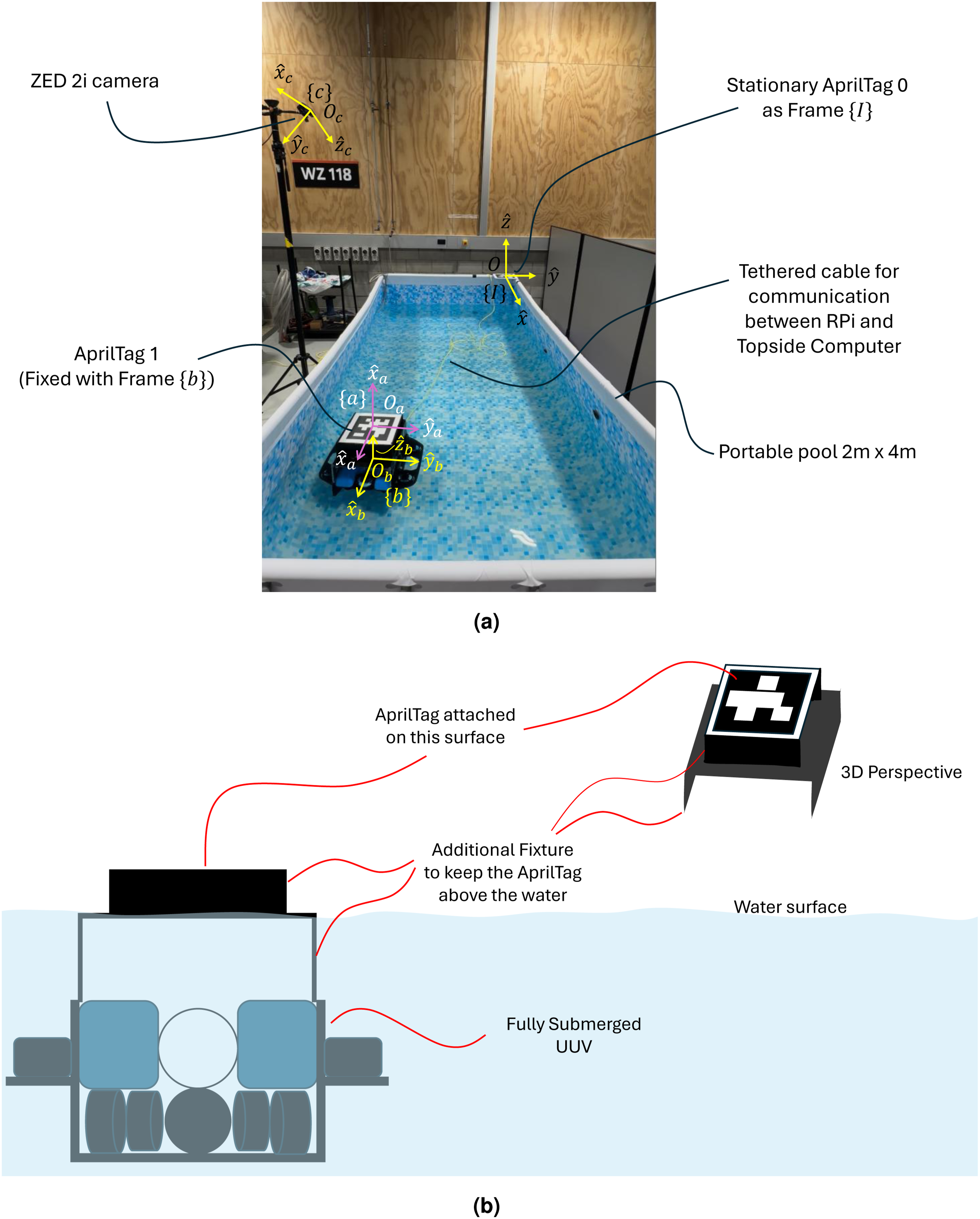
For the experiment, the main challenge is the affordability of a reliable localization system for state-estimation with the sensor suite (e.g., Ultra-Short Baseline (USBL), Doppler Velocity Logger (DVL), Inertial Navigation System (INS)), which usually costs much more than the BlueROV2 Heavy Configuration. Therefore, the AprilTag detection system, which many academic research institutes use to estimate the UUV’s pose (position and orientation), is integrated for the UUV localization (Bauschmann et al., 2023); Jung et al., 2025; Tang et al., 2025). To minimize the computation load on RPi in BlueROV2 Heavy Configuration and to avoid a meticulous installation process of many AprilTags in the pool, the proposed setup consists of only two AprilTags and a ZED 2i camera. This approach eliminates the requirement of accurate measurements among many AprilTags and does not require a particular orientation of the camera as long as both AprilTags can be seen from the ZED 2i camera frame as shown in Figure 11. The experimental pool setup for the UUV localization using AprilTags and the installation of AprilTag on the additional fixture, attached to the UUV, are illustrated in Figure 12. Illustration of the UUV Localization using AprilTags. (a) Experimental Pool Setup for the UUV Localization using AprilTags. (b) Installation of AprilTag on the additional fixture, attached to the UUV.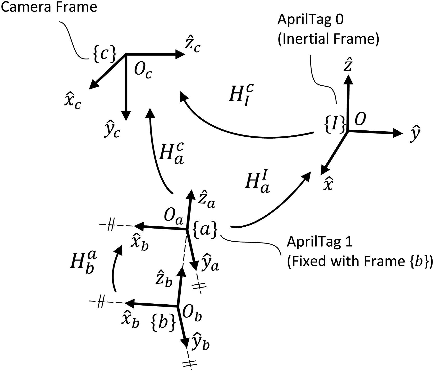
As 
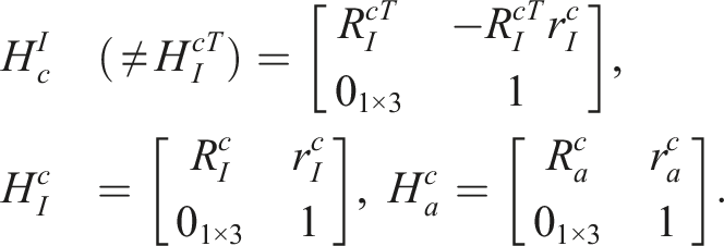
Subsequently, as Frame {b} is fixed in the negative 
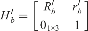
Now, as 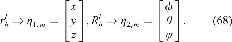
Suppose at time instant i after the time elapse Δt, using the current measured pose 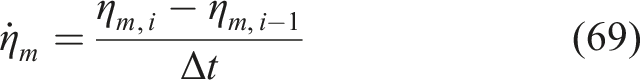
So far, using the AprilTag detection system, the full-state measurements
As the notation conventions, the full states, along with their estimates and the corresponding measured states and their estimates where all of which are represented with respect to and expressed in Frame {I} are denoted as follows: • • • • Other parameters will be described in the same fashion.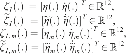
At the time instant i after a time elapse Δt, the state prediction equation can be described as follows:
As all the full states are acquired via the AprilTag detection algorithm and subsequent computation as shown in equation (69), the measurement prediction equation can be written using 
The measurement residual can be obtained by the difference between the actual measurement, ζI,m(i + 1) and measurement prediction as follows:
Given 
Given 
The KF gain can be obtained by
The KF estimated state, that utilizes the latest measurement, can be finally achieved via
Before the next KF loop, the state prediction covariance needs to be updated.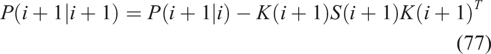
As the full-state estimates from KF are with respect to and expressed in Frame {I} as shown in equation (76) but the UUV’s dynamic model utilizes the twist which is in Frame {b} as shown in equation (2), the rates of change of position and Euler angles (the output of KF) need to be converted into the UUV’s linear and angular velocities. From equation (76), the KF output:
8. Results and discussions
In this section, there are two main subsections: firstly, FNVI Simulations, and secondly, Pool Experiments and Simulations. In each subsection, trajectory tracking, pose (position and orientation) tracking, and energy consumption will be discussed. Subsequently, a summary of the coherent findings between FNVI Simulations and Pool Experiments and Simulations is provided.
For the error comparison, mean-absolute-error (MAE) as shown in equation (78) and MAE ratio as shown in equation (79) will be used.
As shown in Table 1, J T and J E in EO-LQT control consist of the state-varying, input-varying matrix and vector in real-time, unlike CO-LQT control. Therefore, it is tedious to provide how each EO-LQT controller achieves the quantitative measures (MAE, Wh) via the tuning parameters, although it is expected to minimize energy consumption even at the expense of large tracking errors. For instance, CO-LQT1 uses constant Q and R and thus, it can be inferred that these specific values of Q and R result in particular MAE values. However, this inference method does not work for EO-LQT controllers and thus, only MAE ratio comparisons and energy consumptions are directly compared without the directly associated explanation to the tuning parameters in J T and J E . The recorded simulation videos are available at this hyperlink: https://autuni-my.sharepoint.com/:f:/g/personal/jyb1376_autuni_ac_nz/IgD1BjjFhNRRQIlDqYHVQZkJAWmWaM-sAPmGciyF3XaQ1sM.
8.1. FNVI simulations
For FNVI simulation, there are 18 simulations, conducted in total as shown in Table 2. Although the controllers are designed to track a trajectory with 12 reference states (including both pose and twist), only a subset of results is presented for clarity. Specifically, the 3D trajectory tracking performance, the tracking norms for position and orientation, and the energy consumption are reported. This information is sufficient enough to report the trajectory tracking performance and energy-optimality of the proposed controllers, avoiding an overabundance of plots that could overwhelm the overall presentation.
8.1.1. Trajectory tracking: FNVI simulations
The 3D trajectory tracking performance of all controllers are reported in Figure 13. The underwater current disturbance speed direction is illustrated with a black arrow. For a better illustration of 3D trajectory tracking, the 3D view and top views are presented side-by-side. [FNVI Simulation] Trajectory tracking comparison under simulated underwater current speeds.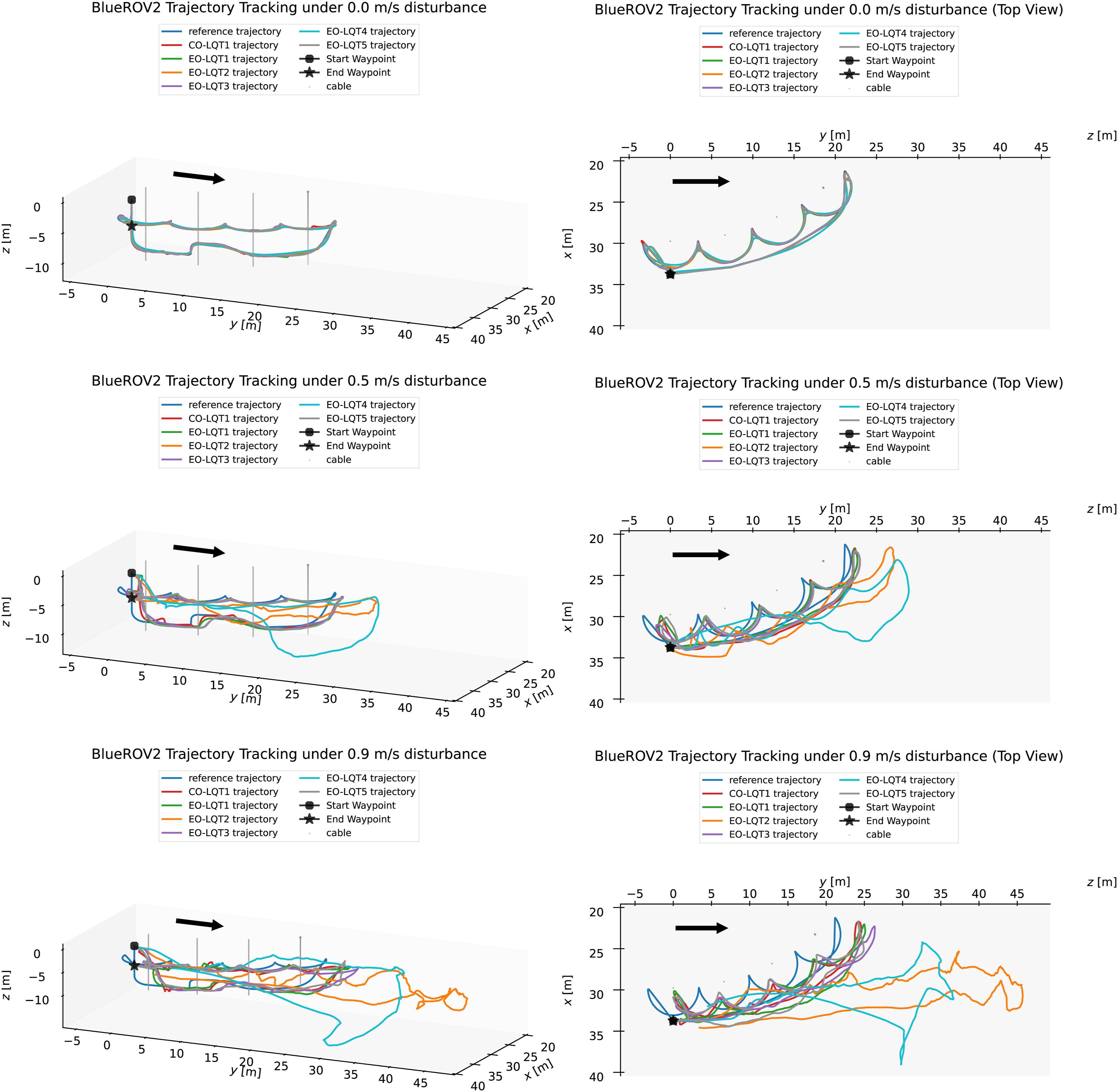
Generally, it can be observed that the tracking performance of EO-LQT2 and EO-LQT4 deteriorates substantially with increasing underwater current speeds, but all other controllers track relatively better than EO-LQT2 and EO-LQT4. In addition to the overall 3D trajectory tracking performance, it is important to quantitatively assess the tracking norms of position and orientation. These metrics will be reported in the following sections.
8.1.2. Pose tracking: FNVI simulations
[FNVI Simulation] Pose tracking error norm and energy consumption comparison taking CO-LQT1 as the baseline.
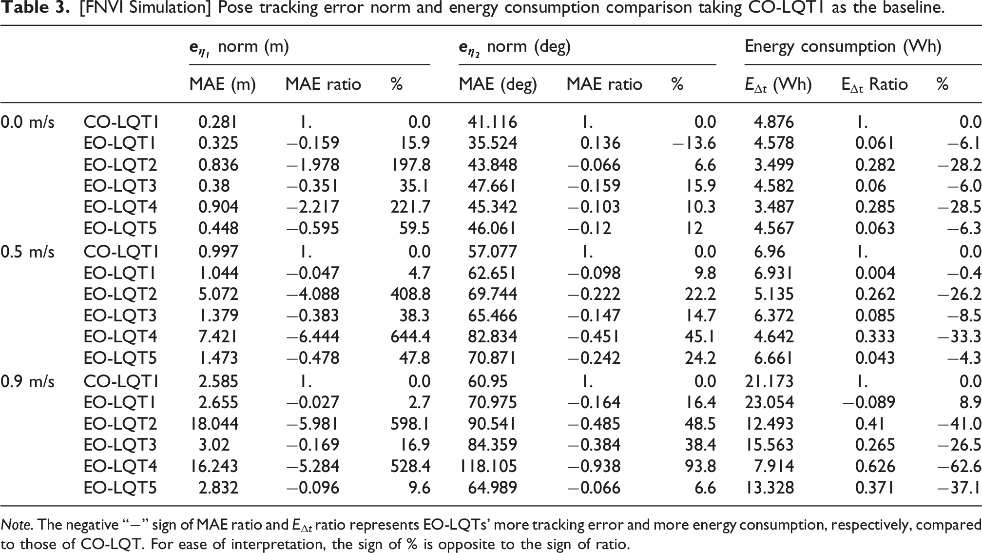
Note. The negative “−” sign of MAE ratio and EΔt ratio represents EO-LQTs’ more tracking error and more energy consumption, respectively, compared to those of CO-LQT. For ease of interpretation, the sign of % is opposite to the sign of ratio.
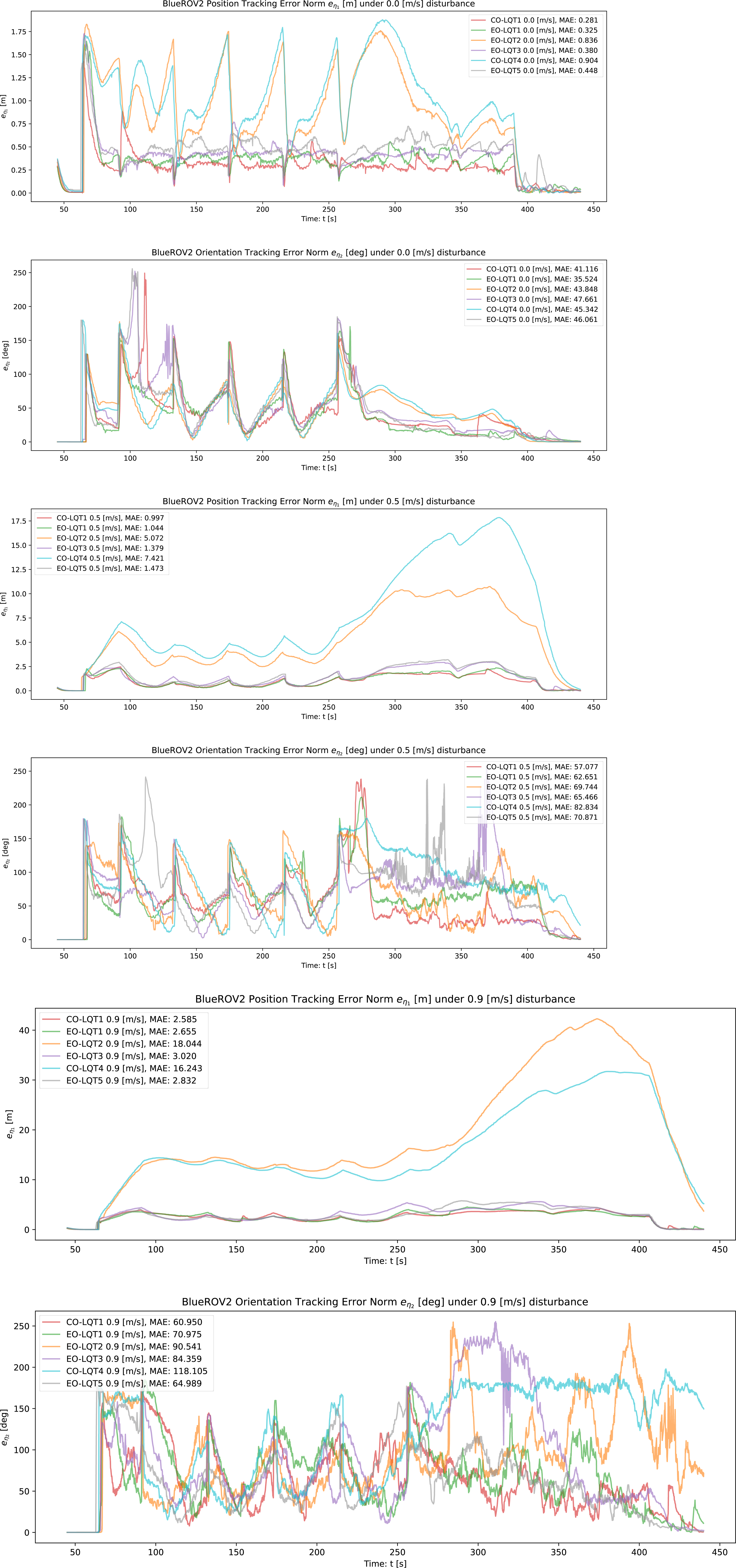
[FNVI Simulation] Pose tracking error norm comparison under simulated underwater current speeds.
Although the MAE % provides a quantitative measure for comparing the relative pose tracking performance among controllers, the selection of a controller should not rely solely on this metric. Instead, practical considerations—such as whether a given MAE value is acceptable for the intended application—should also guide the decision-making process. For instance under 0.9 m/s disturbance speed for a particular FNVI operation, if the MAE value of 2.832 m (EO-LQT5) is acceptable, compared to that of 2.585 m (CO-LQT1), the selection of EO-LQT5 is a better choice, supposed if it saves more energy. Hence, another evaluation metric for controller selection is energy consumption.
8.1.3. Energy consumption: FNVI simulations
The energy consumptions of the controllers under simulated underwater current speeds are plotted in Figure 15. Their respective EΔt Ratio and energy saving % are reported in Table 3. Generally as expected, all EO-LQTs save more energy than CO-LQT in an ideal scenario without any underwater current disturbance speed. EO-LQT1’s energy saving performance deteriorates under increasing disturbance speeds. EO-LQT2 and EO-LQT4 save more energy substantially under increasing disturbance speeds at the expense of very large pose tracking error as shown in Figure 13. Both EO-LQT3 and EO-LQT5 save energy regardless of the increasing disturbance speeds. Based on the % metric of [FNVI Simulation] Energy consumption comparison tested under simulated underwater current speeds.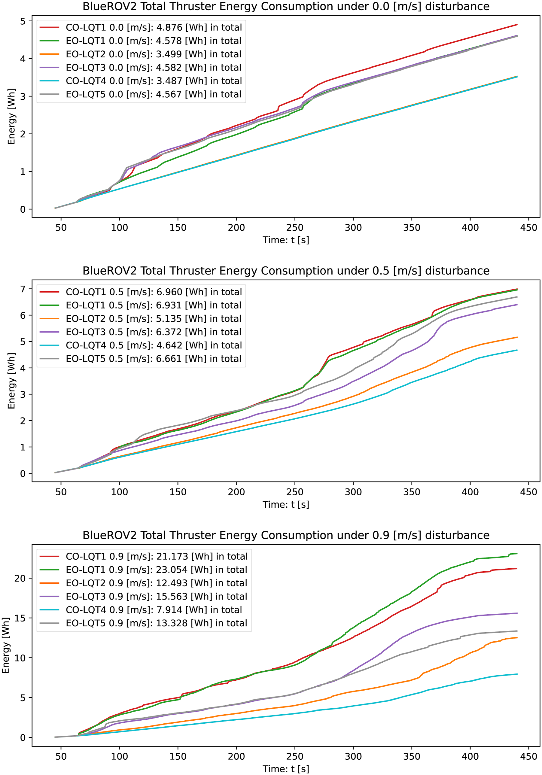
8.2. Pool experiments and simulations
Using the vision-based state-estimation, detailed in Subsection 7.1, all proposed controller are tested on the actual hardware of BlueROV2 Heavy Configuration in the pool as shown in Figure 12. Similarly, simulations are conducted with the same trajectory as the pool experiment.
In a similar fashion to FNVI simulations, the 2D trajectory tracking performance, the tracking norms for position and orientation, and the energy consumption of pool experiments and simulations are reported in this subsection. In addition, it is important to note that there are a few factors that can cause model uncertainties in addition to the unmodeled dynamics in the actual experiments. Some important factors are listed as follows: • The UUV is mounted with the additional corrugated plastic sheets to attach AprilTag for the vision-based state-estimation system. Although the weight can be considered negligible, the corrugated plastic sheets sealed with glue may introduce additional buoyancy, and it could potentially increase hydrodynamics parameters, especially for yaw motion. • The additional weight, tension, and drag introduced by the tethered cable could potentially affect the overall dynamics of the UUV. • Due to the requirement of the vision-based state-estimation system and the slight positive buoyancy, the UUV operates around the water surface level, although its main body is fully submerged underwater. Therefore, the near-surface operation could potentially affect the overall dynamics of the UUV.
8.2.1. Trajectory tracking: Pool experiments and simulations
The 2D trajectory tracking performance of all controllers is reported in Figure 16. In both pool experiments and simulations, inferior tracking performance is observed for EO-LQT2 and EO-LQT4 compared to the other controllers. While the differences in trajectory tracking performance among other LQT controllers are not particularly substantial in the pool simulations, they are notably more evident in the pool experiments. [Pool Experiments and Simulations] Trajectory tracking comparison (top view).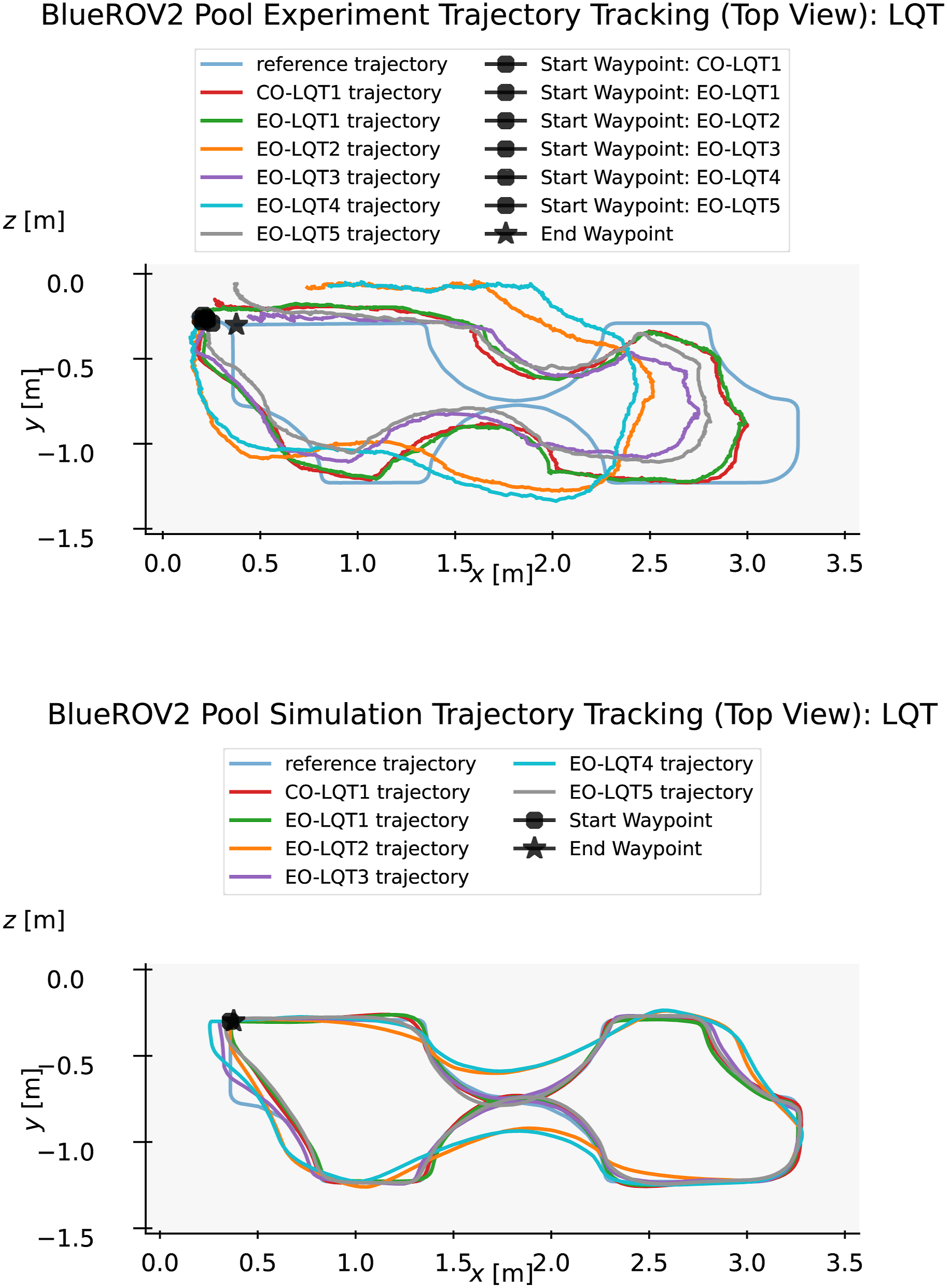
There are a few important observations between pool experiments and simulations. Firstly, unlike in simulations, it is challenging to maintain the UUV at a fixed position (Start Waypoint) in the pool prior to the activation of the controllers, resulting in multiple start waypoints as shown in Figure 16. Secondly, due to the aforementioned start waypoints drifted to the left (in the negative direction of x axis), the resulting UUV’s trajectory is also shifted to the left. The quantitative performance measures will be detailed in the following.
8.2.2. Pose tracking: Pool experiments and simulations
The pose tracking error norms of pool experiments and simulations are plotted in Figure 17. The pose tracking error norms and its ratio are reported in Table 4. Due to the drift to the left (in the negative direction of x axis), there are substantial difference in position tracking error norm at the start and the overall position tracking error norm profile is shifted to the left. Most likely due to model uncertainties and unmodeled dynamics mentioned earlier and experimental setup for the start waypoint, the respective [Pool Experiments and Simulations] Pose tracking error norm comparison. [Pool Experiments and Simulations] Pose tracking norm and energy consumption comparison taking CO-LQT1 as the baseline. The negative “−” sign of MAE ratio and EΔt ratio represents EO-LQTs’ more tracking error and more energy consumption, respectively, compared to those of CO-LQT. For ease of interpretation, the sign of % is opposite to the sign of ratio.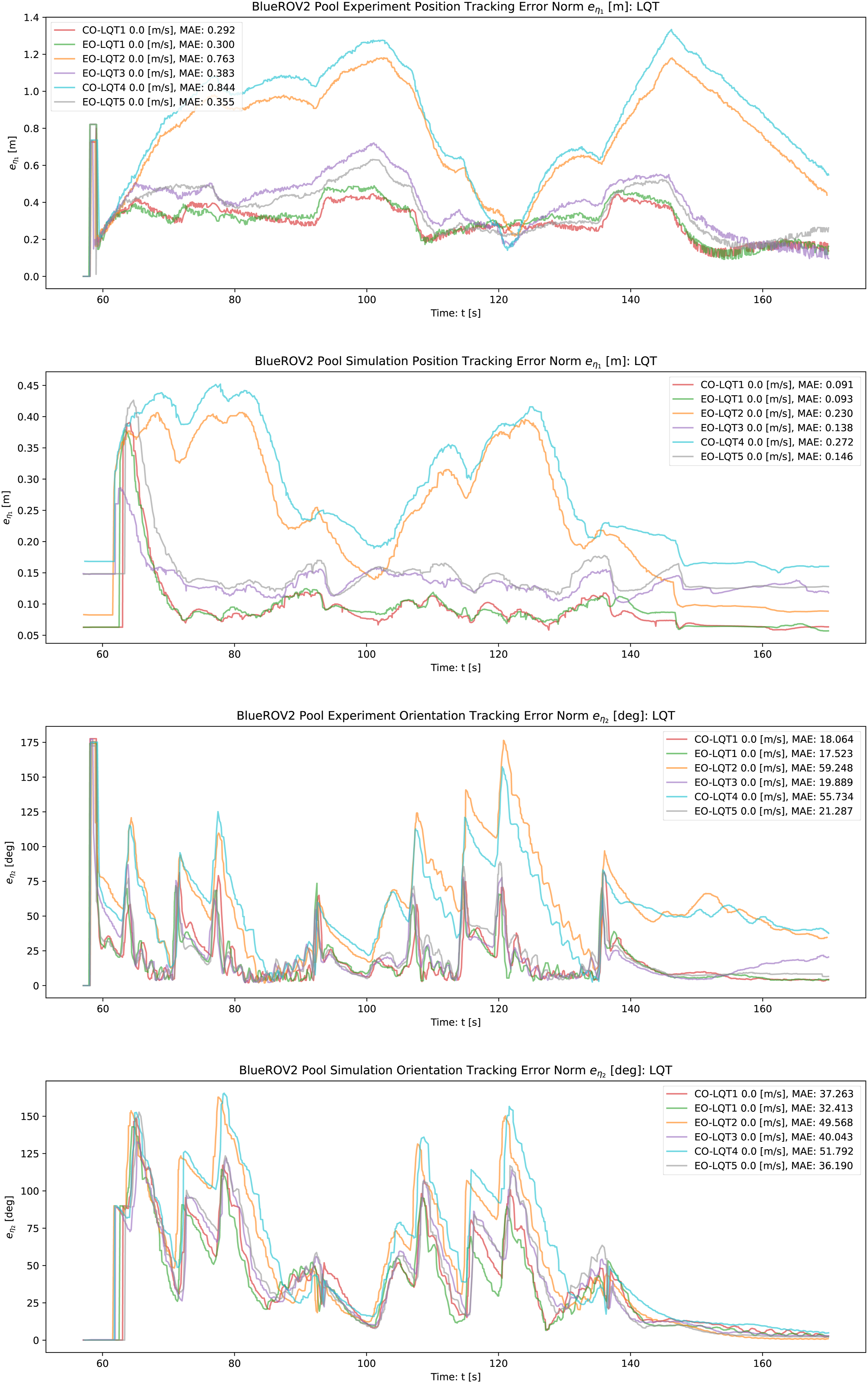
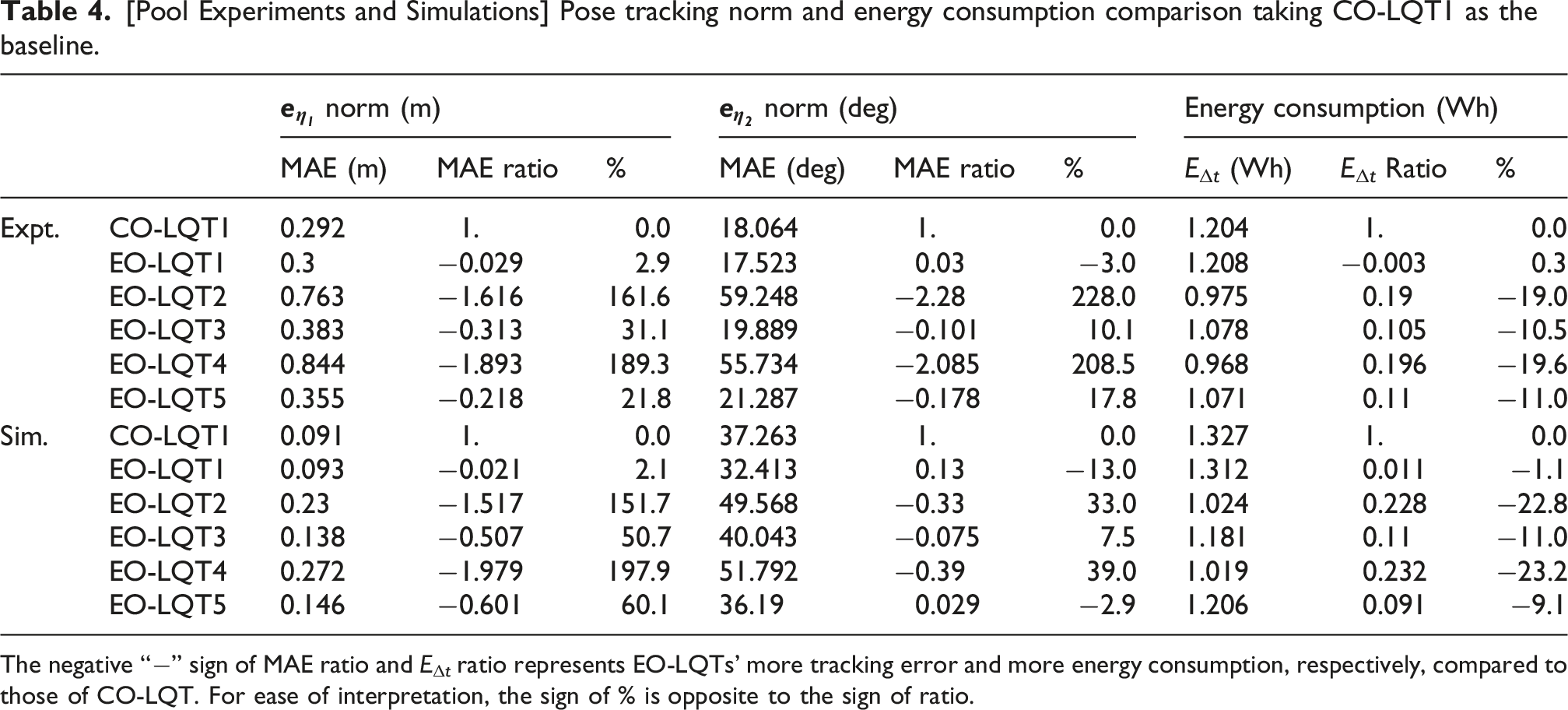
Similar to the position tracking error norm, a substantial difference in the orientation tracking error norm is observed at the beginning. Likewise,
Generally, the overall pose tracking performances of all controllers, especially including the baseline CO-LQT, are different in pool experiments and simulations. Based on this observation, it can be inferred that the main performance difference of the controllers during pool experiments and simulations is not due to the incoherent behaviors of the proposed controllers but because of the aforementioned model uncertainties, unmodeled dynamics, and experimental setup for the start waypoint, affecting all controllers.
In addition to the coherent profiles of MAE % of
8.2.3. Energy consumption: Pool experiments and simulations
As shown in Figure 18, the overall energy consumption profiles of the controllers during pool experiments and simulations are substantially similar. As reported in Table 4 and based on pose tracking performance differences discussed earlier, the energy consumption values of the controllers in both pool experiments and simulations are considered reasonable and consistent. Although EO-LQT1 consumes a negligible amount of more energy (0.3 %) in pool experiments, the overall energy consumption profiles of all controllers are coherent across pool experiments and simulations. With the consideration of energy consumption among EO-LQT1, EO-LQT3 and EO-LQT5, which are identified to achieve superior pose tracking performance earlier, EO-LQT3 and EO-LQT5 are the most energy-optimal trajectory tracking controllers. [Pool Experiments and Simulations] Energy consumption comparison.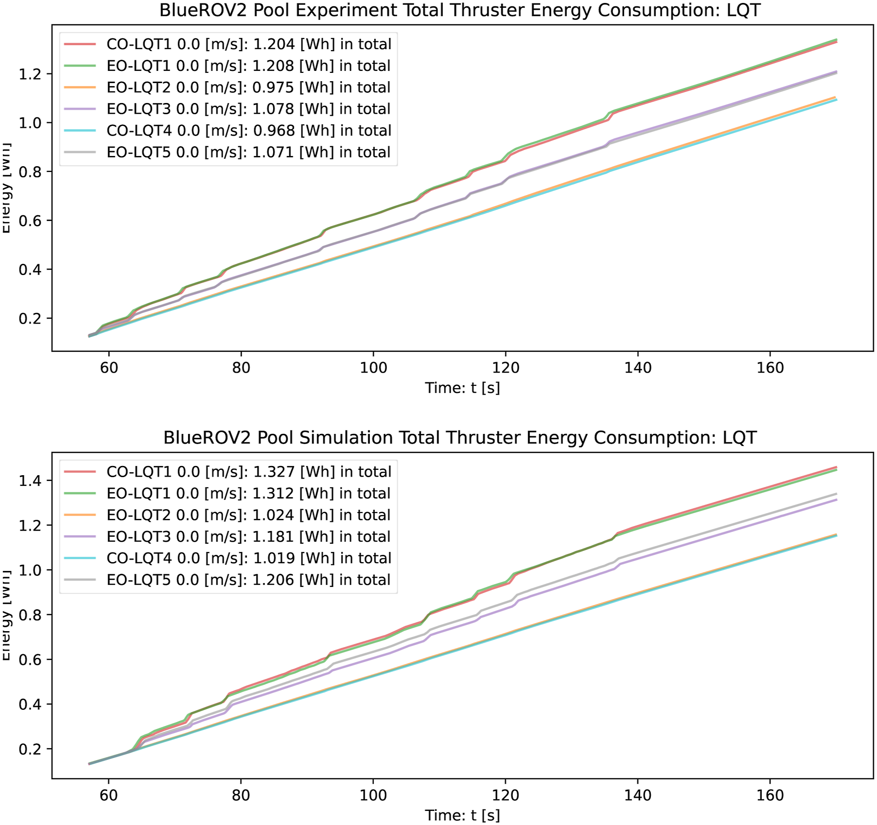
8.3. Inferring future FNVI field trial outcomes from pool experiments and simulations
Based on the earlier discussion on pose tracking and energy consumption of pool experiments and simulations, it is obvious that the MAE values of pose tracking and energy consumption of controllers are substantially different between pool experiments and simulations. Given that even the baseline CO-LQT exhibits the same phenomenon, it can be concluded that these substantial differences between pool experiments and simulations arise from model uncertainties, unmodeled dynamics and variations in the starting waypoint within the experimental setup. On the other hand, the respective overall profiles of MAE values of pose tracking and energy consumption of controllers are coherent between pool experiments and simulations. Given these coherent profiles between pool experiments and simulations, the next intriguing question is whether any plausible conclusion can be drawn between the pool experiments and FNVI simulations.
As shown in Tables 3 and 4, the MAE % profiles of pose tracking of controllers without disturbances in FNVI simulations are coherent with those in pool simulations. Likewise, energy consumption % profiles of controllers between FNVI simulations and pool simulations are similar. Given this coherent observation among pool experiments, pool simulations and FNVI simulations, it can be inferred that the experimental results of the proposed controllers in future FNVI field trials are likely to align with the findings from the pool experiments. Therefore, EO-LQT3 and EO-LQT5 are most likely to be the suitable energy-optimal trajectory tracking controllers, but there are substantial future works to be done before the field trials in the open ocean. The potential future works will be detailed in the following section.
9. Future work
Given the results of EO-LQT3 and EO-LQT5 under different underwater current disturbance speeds (e.g., 0.0 m/s - 0.9 m/s), they relatively perform the trajectory tracking well, while minimizing the energy consumption. However, the performance differences between pool experiments and simulations underline the plausible factors, highlighted in Subsection 8.2, which can cause model uncertainties in addition to the unmodeled dynamics. Therefore, future work directions are related to minimizing those factors via hardware upgrades and are targeted to field trials, exploring more energy-optimal control schemes with stability and robustness analysis. • Although the current experimental setup requires only one camera and two AprilTags, the additional fixture is needed to keep the fixed AprilTag on the UUV above the water. This fixture potentially increases hydrodynamic parameters and the overall UUV dynamics (model uncertainties and unmodeled dynamics). Therefore, to remove this additional fixture, the experimental setup should be changed to multiple AprilTags inside the pool and one low-light camera (with high resolution and high frames per second) mounted on the UUV dedicated to localization. • Relating to the use of multiple AprilTags inside the pool, it requires a real-time localization strategy for state-estimation, which does not rely heavily on the accuracy of the physical installation of multiple AprilTags. • Currently, the tethered cable is used for communication to transfer data between the topside computer and the UUV. The topside computer performs AprilTag detection, vision-based full state-estimation, and control algorithm executions. To achieve a tetherless operation, the UUV needs to perform all those tasks onboard and thus, it needs to be upgraded with higher computing capacities. • In addition to achieving a tetherless UUV with high computing capacities onboard, a proper identification of the hydrodynamic and hydrostatic parameters of the UUV needs to be carried out on the new form-factor due to the hardware upgrade. • After conducting the extensive controller experiments on BlueROV2 Heavy Configuration with the aforementioned hardware upgrade in the controlled environment, a larger industrial-grade UUV is required for the open ocean field trials in the future.
10. Conclusion
In this paper, the energy-optimal control schemes based on linear quadratic tracking (LQT) principles are developed for a UUV performing the FNVI task of the Blue Endeavour Project (the first of its kind for offshore aquaculture salmon farm in New Zealand) of New Zealand King Salmon Company. The linearized model in the form of an LPV system is produced via factorizing the nonlinear UUV dynamic model and extracting states using the proposed modified versions of Bhāskara I’s sine approximation and Shirali’s cosine approximation. Subsequently, the Lagrangian
Several variants of EO-LQT controllers are proposed and tested on a lightweight and highly maneuverable UUV, called BlueROV2 Heavy Configuration, in ROS-based high-fidelity simulation platform integrated with Gazebo Physics Engine called UUV Simulator under three underwater current speeds (0.0 m/s, 0.5 m/s, and 0.9 m/s). The proposed controllers are also tested on the actual hardware of BlueROV2 Heavy Configuration in the pool, along with their respective high-fidelity simulation tests in the pool environment.
From the analysis on trajectory tracking accuracy and energy-optimality, EO-LQT3, which uses a non-quadratic power function of T200 thruster, and EO-LQT5, which uses the Lagrangian
Footnotes
Acknowledgments
The authors acknowledge the financial support of the Blue Economy Cooperative Research Centre, established and supported under the Australian Government’s CRC Program, grant number CRCXX000001 (previously 20180101). The CRC Program supports industry-led collaborations between industry, researchers and the community. The authors also acknowledge the graduate research facilities and the financial support of the Auckland University of Technology (AUT) in providing the waiver of the PhD tuition fees. We greatly appreciate the technical support of Mr. Simon Hartley, the technical specialist-mechatronics at AUT, Mr. Adam Poloha, the research assistant at Mechatronics Lab, AUT and Mr. Sai Htet Moe Swe, my fellow PhD student at AUT.
Funding
The authors disclosed receipt of the following financial support for the research, authorship, and/or publication of this article: This research project is supported by the Blue Economy Cooperative Research Centre, established and supported under the Australian Government’s CRC Program, grant number CRCXX000001 (previously CRC-20180101).
Declaration of conflicting interests
The authors declared no potential conflicts of interest with respect to the research, authorship, and/or publication of this article.
Note
Appendix
Hardware and software specification for ROS.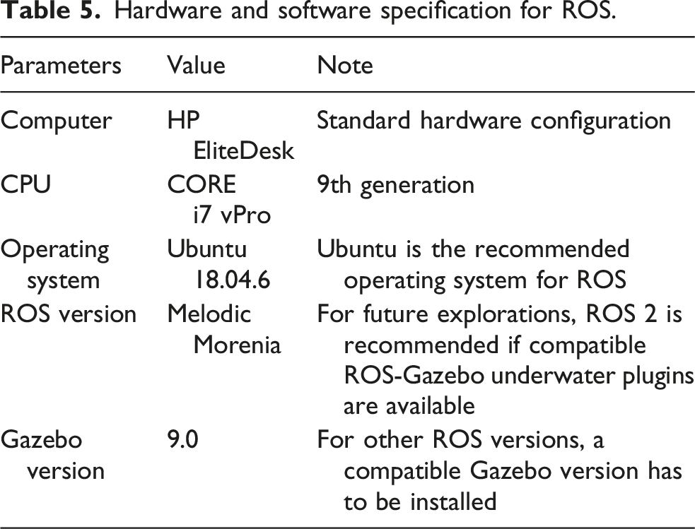
Parameters
Value
Note
Computer
HP EliteDesk
Standard hardware configuration
CPU
CORE i7 vPro
9th generation
Operating system
Ubuntu 18.04.6
Ubuntu is the recommended operating system for ROS
ROS version
Melodic Morenia
For future explorations, ROS 2 is recommended if compatible ROS-Gazebo underwater plugins are available
Gazebo version
9.0
For other ROS versions, a compatible Gazebo version has to be installed