
Abstract
Active perception is a fundamental problem in autonomous robotics in which the robot must decide where to move and what to sense in order to obtain the most informative observations for accomplishing its mission. Existing approaches either solve a computationally expensive traveling salesman problem over heuristically selected informative nodes, or adopt a more efficient but overly constrained shortest path tree formulation. To address these limitations, we explore beam search algorithms as scalable alternatives. While the standard beam search provides scalability by preserving the top-B paths at each depth level, it is prone to local optima and exhibits parameter sensitivity. Our first contribution is a node-wise beam search (NBS) algorithm, which maintains top-B candidates per node to enable more effective exploration of the solution space. Systematic benchmarking on graphs shows that NBS consistently outperforms other baselines and maintains strong performance even at low beam widths. As a second contribution, we integrate the concept of frontiers into the path selection criterion, introducing the expected gain metric, which better balances exploration and exploitation compared to existing alternatives. Our third contribution proposes the rapidly-exploring random annulus graph (RRAG), a novel graph construction method that preserves full orientation sampling and ensures connectivity in cluttered environments through a fallback local sampling-based planner. Extensive experiments demonstrate that NBS combined with RRAG achieves the highest performance across all three representative active perception tasks, outperforming state-of-the-art algorithms by at least 20% in one or more tasks. We further validate the approach on real robotic platforms in different scenarios. Project page: https://efficient-beam-search.github.io/
Keywords
1. Introduction
Autonomous robots are increasingly deployed for tasks requiring intelligent information gathering, such as environment monitoring (Cao et al., 2013; Ghaffari Jadidi et al., 2019; Popović et al., 2020; Singh et al., 2009; Yu et al., 2016), autonomous exploration (Bircher et al., 2016b; Cao et al., 2021; Meng et al., 2017; Zhou et al., 2021), and surface reconstruction (Bircher et al., 2015; Kompis et al., 2021; Schmid et al., 2020; Yoder and Scherer, 2016). Unlike conventional shortest path planning, which aims to minimize traversal cost to reach a goal, these applications pose a more complex challenge: how to enable robots to autonomously plan sensor trajectories that maximize accumulated information under resource constraints such as time or energy.
Furthermore, robots often operate under partial observability, with neither the environment nor the information distribution known a priori. This motivates active perception scenarios, where the robot must simultaneously explore the environment and plan informative trajectories in the free space. Sampling-based planners such as rapidly-exploring random tree (RRT) and RRT* (Karaman and Frazzoli, 2010; Kuffner and LaValle, 2000) have been adapted to this setting (Bircher et al., 2016b; Moon et al., 2022). However, tree-based structures have inherent limitations: each node stores only one incoming path, and extensive rewiring or pruning is required as the robot moves, often leading to degraded solution quality or high computational overhead.
Graph-based representations offer greater flexibility through multi-query planning capabilities. Since planning the most informative path on a graph is NP-hard (Ahuja et al., 1983), prior work has employed simplifying heuristics, such as restricting the search to a shortest path tree (SPT) (Dang et al., 2020; Xu et al., 2021). While computationally efficient, this severely limits the search space. Another common approach decouples node selection from routing: informative nodes are selected or sampled heuristically and then connected via shortest paths using a traveling salesman problem (TSP) solver (Arora and Scherer, 2017; Meng et al., 2017; Zhou et al., 2021). However, this separation often leads to suboptimal paths and high computational cost.
In this work, we adopt the term informative path planning (IPP) to refer broadly to graph-based path planning problems that seek a path maximizing a given gain metric subject to a cost budget. Importantly, we do not address information-theoretic objectives, such as those in Bai et al. (2016), Chen et al. (2024a), Lim et al. (2016), and Singh et al. (2009), but instead treat IPP as a path optimization problem defined over a graph.
Given the combinatorial nature of IPP, we turn to beam search—a well-established algorithm in sequential decision-making (Meister et al., 2020; Rush et al., 2013; Vijayakumar et al., 2018). It strikes a balance between the efficiency of greedy search and the optimality of exact inference by iteratively pruning the search space to focus only on the most promising partial solutions. We first explore the standard variant, termed depth-wise beam search (DBS), which maintains the top B paths at each search depth. Although more flexible than SPT- or TSP-based methods, this approach remains sensitive to parameter choices and prone to local optima. To address these limitations, we propose node-wise beam search (NBS), which maintains the top B paths per node. This design enhances robustness to parameter variation and enables more effective exploration of the search space.
We first benchmark path planning algorithms in two abstract graph settings: planning informative paths on a fully known graph and on a graph incrementally discovered from sensor data. Most algorithms require a path selection criterion, that is, a metric that generalizes across both settings for ranking candidate paths. The two most commonly used metrics are path gain and path ratio (gain-to-cost ratio). To better balance exploration of new information against exploitation of known gains, we introduce the expected gain metric, which incorporates frontier (Yamauchi, 1997) information to estimate potential future gains. Through extensive evaluations, we show that NBS consistently outperforms TSP, SPT, and DBS on graphs. Our proposed expected gain criterion achieves a superior balance between exploration and exploitation compared to existing metrics. We also observe that frequent replanning further improves performance, especially in online perception settings.
Transitioning from graph environments to active perception requires online and incremental graph construction. To this end, we propose rapidly-exploring random annulus graph (RRAG), an incrementally built graph structure inspired by rapidly-exploring random graph (RRG) (Karaman and Frazzoli, 2011). The name annulus graph reflects its spacing rules: nodes are accepted only if sufficiently distant from existing ones, and edges are formed only when nodes are within a suitable proximity, preventing excessive node density and edge connectivity. Unlike previous incremental graph construction methods that retain a single orientation per position (Schmid et al., 2020; Xu et al., 2021), RRAG preserves multiple orientations, enhancing directional coverage. Moreover, while most approaches assume straight-line edges—which often fail in narrow or cluttered environments—RRAG introduces a fallback local sampling-based planner to ensure connectivity even in highly constrained spaces.
We validate our approach through comprehensive simulations on three representative active perception tasks: point collection, surface reconstruction, and volumetric exploration, across eight scenarios from the Habitat Synthetic Scenes Dataset (HSSD) (Khanna et al., 2024). NBS combined with RRAG achieves the highest performance in all three tasks, outperforming state-of-the-art methods by at least 20% in one or more tasks. These results, complemented by real-world robotic experiments (see Figure 1 for an example), demonstrate the effectiveness and generalizability of our approach. Alongside this work, we release Surface reconstruction in hardware experiments. The figure illustrates the robot’s navigation sequence alongside the corresponding reconstructed scene. The completed trajectory is visualized with a color gradient from dark blue to bright yellow, while the currently planned path is shown as a sequence of light green arrows. The camera’s view frustum is depicted, and yellow voxels represent surface frontiers visible within it. Each node is represented by a color-coded arrow: low-gain nodes are blue, and high-gain nodes are red. The bottom left panel illustrates the planning pipeline: the planner identifies the optimal path using NBS and, upon reaching the next node, updates and expands the graph with new information before computing the next-best path.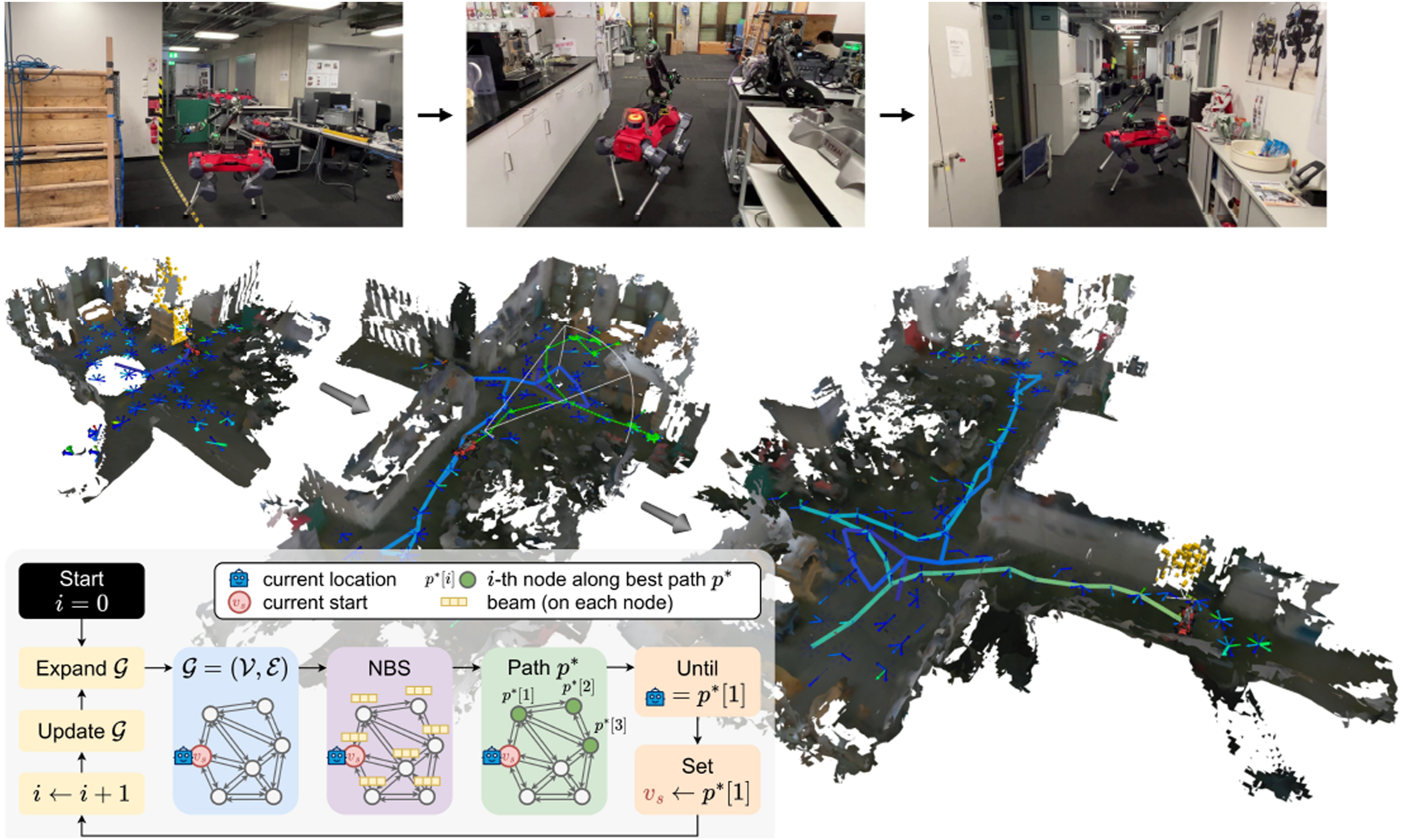
We summarize our main contributions as follows: (1) We propose NBS, an efficient node-wise beam search algorithm that maintains a bounded set of top candidate paths per node. Extensive experiments demonstrate that NBS is robust to parameter choices and consistently outperforms state-of-the-art approaches in both graph environments and active perception tasks. (2) We integrate frontier information into the path selection criterion by introducing the expected gain metric, which balances exploration of unknown space and exploitation of gains in free space. Empirical results show that this formulation surpasses other alternatives, such as path ratio, across a variety of graph environments. (3) We introduce RRAG, a novel incremental graph construction method for active perception. RRAG preserves multiple orientations at each position, enabling richer path optimization. It also incorporates a fallback local sampling-based planner to ensure graph connectivity in cluttered environments.
This paper is structured to progressively build both intuition and formal understanding of the proposed approach. Section 2 reviews relevant prior work in active perception, autonomous exploration, informative path planning, and sampling-based planning. Section 3 formulates the active perception problem across three increasingly realistic settings: planning on a fully known graph, planning on an incrementally discovered graph, and active perception with incremental environment exploration. Section 4 introduces key components such as path selection criteria and replanning strategies, and discusses properties of optimal paths. Section 5 presents different IPP algorithms, including the proposed NBS algorithm, along with theoretical analysis of their computational complexity. Section 6 evaluates the proposed methods against established baselines in different graph environments. Section 7 details RRAG, our incremental graph construction method that enables the application of IPP algorithms to active perception. Section 8 presents empirical results from extensive simulations and real-world robotic experiments, demonstrating the effectiveness of our approach in active perception tasks. Finally, Section 9 discusses limitations and future work, and Section 10 concludes the manuscript. An overview of the paper’s structure is provided in Figure 2. Paper organization overview. Circled numbers indicate the corresponding sections. In the graph a priori and online perception settings, the environment is represented as a graph, either fully known or partially known. In contrast, active perception necessitates graph construction from the collision-free state space. The path selection strategy encompasses both selection criteria and replanning frequencies, which are benchmarked in the graph-based settings. The best-performing combination is subsequently applied to the active perception tasks.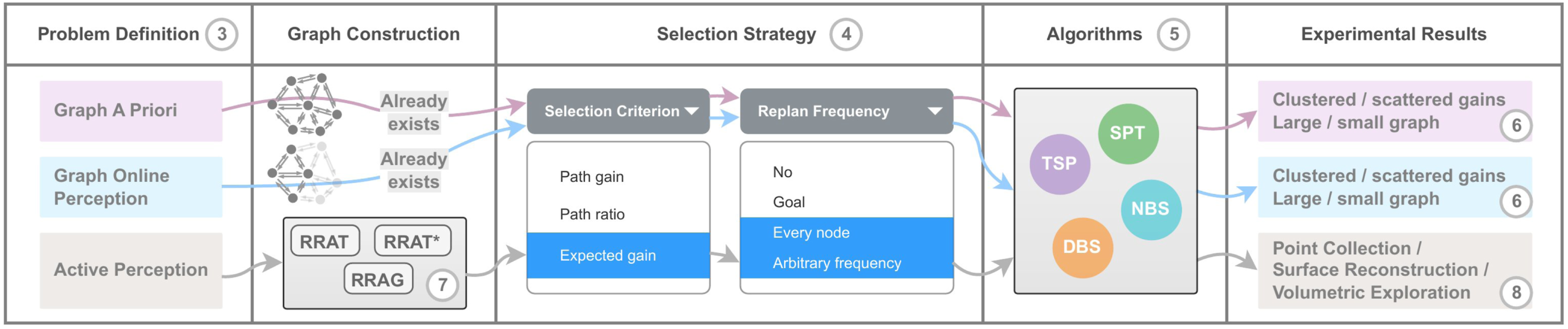
2. Related work
One of the most fundamental active perception tasks is autonomous exploration, in which a robot aims to explore as much of the environment as possible. A seminal approach is frontier-based exploration (Yamauchi, 1997), where the robot repeatedly navigates to the boundaries between known free space and unknown regions to incrementally complete a map. Subsequent work has addressed the challenge of high-speed exploration on multi-rotor platforms (Cieslewski et al., 2017). Building on the frontier concept, recent methods have integrated TSP-style formulations to achieve more globally efficient exploration policies. FUEL (Zhou et al., 2021) incrementally maintains a frontier information structure (FIS) by computing axis-aligned bounding boxes for frontier clusters and then solving an asymmetric TSP to generate a global tour that visits representative viewpoints. RACER (Zhou et al., 2023) extends FUEL to multi-UAV settings and uses coverage paths to guide exploration while avoiding repeated visits to the same regions. Other works, however, argue against casting exploration directly as a TSP problem. FAEL (Huang et al., 2023) introduces heuristic strategies that solve a path optimization problem jointly considering movement distance, information gain, and coverage. Yu et al. (2023) proposed ECHO, an efficient heuristic for next viewpoint determination that selects the next viewpoint via a lightweight cost function accounting for boundary awareness, environmental structure, and motion consistency, achieving both computational efficiency and improved performance.
Recently, many researchers have explored applying IPP formulations to a wide range of active perception problems. The objective of informative path planning is to compute a path that maximizes information gain while satisfying a given cost budget. Classical IPP formulations typically assume a fully known environment represented as a weighted graph, where vertices encode information gains and edges represent traversal costs (Lim et al., 2016; Singh et al., 2009). A major application is environment monitoring, where Gaussian processes are commonly used to model uncertainty and guide planning to reduce terrain uncertainty (Chen et al., 2024a; Ma et al., 2018; Popović et al., 2020; Singh et al., 2009). Yu et al. (2016) employ a mixed-integer quadratic program to solve the planning problem, while Ott et al. (2024) introduce an approximate sequential path optimization method that constructs trajectories segment by segment using dynamic programming. More recently, Jakkala and Akella (2025) propose a fully differentiable IPP formulation that offers significant gains in speed and scalability. Reinforcement learning-based approaches have also attracted increasing attention (Cao et al., 2023; Rückin et al., 2022). Beyond known environments, several works extend IPP to unknown settings for autonomous exploration and active mapping (Asgharivaskasi et al., 2022; Bai et al., 2016; Chen et al., 2024b; Ghaffari Jadidi et al., 2019).
To optimize information gain under a cost budget, one major line of work adopts a TSP-based approach: sampling a set of candidate nodes and then using established TSP solvers to determine an efficient visitation sequence. Arora and Scherer (2017) first applied TSP to generate a route through all sampled nodes and then iteratively evaluated the effect of adding or removing nodes to further improve the solution. This method leverages mature TSP solvers but assumes a predetermined endpoint, limiting its applicability in realistic scenarios. Meng et al. (2017) improved upon this by eliminating the dependency on a fixed endpoint and incorporating a heuristic cost function to accelerate the optimization. Cao et al. (2021) adopted a hierarchical framework, applying TSP both within a local planning horizon to sequence dense viewpoints and at the global level to visit sparse sub-spaces. Similar ideas appear in structural inspection and surface coverage tasks. Bircher et al. (2015, 2016a) proposed generating a minimal set of viewpoints that collectively cover a structure (analogous to the Art Gallery Problem (Lee and Lin, 1986)), then solved the TSP to connect them. Rather than solving the Art Gallery Problem directly, they used multiple iterations of random sampling to refine the solution. The TSP-based paradigm has two key limitations. First, it employs a two-stage optimization: candidate nodes are selected (or sampled) first, and only afterward is a near-optimal tour computed—sequencing and node selection are not jointly optimized under the cost constraint. Second, TSP quickly becomes computationally prohibitive as the number of candidate nodes increases, limiting its scalability.
Another mainstream approach to applying the IPP formulation in active perception is via sampling-based planning. In this paradigm, a tree or graph is incrementally grown in the free space, with the information gain of each sampled node evaluated to ultimately extract the most informative path. Sampling-based planning has become the de facto standard for path planning in high-dimensional configuration spaces. These methods avoid the explicit construction of obstacles, instead relying on collision-checking modules to build a connectivity graph or tree. Kavraki et al. (1996) proposed the probabilistic roadmap (PRM), which constructs a persistent graph of the free space, enabling efficient multi-query planning. For single-query problems, the RRT was developed (LaValle, 1998; LaValle and Kuffner Jr., 2001), which utilizes a Voronoi bias to rapidly expand a tree from the start state toward the goal. Several extensions improve planning efficiency, such as RRT-Connect (Kuffner and LaValle, 2000), which grows two trees simultaneously (from the start and the goal), and expansive space trees (EST) (Hsu et al., 1997), which bias expansion toward sparsely explored regions. To address the suboptimality of these early approaches, Karaman and Frazzoli (2011) introduced the RRG and its tree-based counterpart, RRT*, both of which are asymptotically optimal. RRT* employs a rewiring mechanism to dynamically maintain the lowest-cost parent for each node while preserving a tree structure. RRT X (Otte and Frazzoli, 2016), another asymptotically optimal algorithm that grows from the goal toward the start, was proposed to enable real-time replanning in dynamic environments. However, these seminal sampling-based planners focus on finding the shortest path to a goal in a fully known environment and do not inherently address mapping or information-gathering objectives.
Recently, RRTs have been adapted to extend traditional motion planning algorithms to active perception tasks. Bircher et al. (2016b) adapted RRTs for exploration by sampling viewpoints to construct a tree and selecting the branch with the highest gain, with a weight affected by the cost, for execution. After each planning step, only the selected immediate branch is retained, and the tree is re-expanded. This approach has been further extended to surface inspection in unknown environments (Bircher et al., 2018). Witting et al. (2018) proposed sampling from pruned nodes to rapidly recover node density. Schmid et al. (2020) enhanced this method by rewiring the non-executed branch to the new root, enabling direct reuse of previously sampled nodes, following the connection strategy in RRT* (Karaman and Frazzoli, 2011). To address large and high-dimensional search spaces, Kompis et al. (2021) and Moon et al. (2022) introduced informed sampling strategies to sample nodes with high expected information gain. Tree-based planners inherently sacrifice optimality due to the limited number of candidate paths and the need for frequent tree updates. Additionally, shortest-path formulations typically exclude repeated nodes, whereas revisiting nodes can be beneficial.
Graph-based algorithms relax the constraint of maintaining a single path to each node by constructing a graph representation of the environment and searching for informative paths within it. Moreover, such approaches are inherently better suited for online replanning, as they do not rely on a rooted structure and thus eliminate the need for tree rewiring. Xu et al. (2021) and Duberg and Jensfelt (2022) propose incrementally constructing a graph during exploration. GBPlanner (Dang et al., 2020) introduced a dual-graph structure for large-scale exploration, where local graphs are built within bounded regions and incrementally merged into a global graph. All these methods reduce the search space by applying shortest-path algorithms (e.g., Dijkstra) over selected nodes to generate shortest-path trees, effectively transforming the problem into a tree search embedded in an underlying graph. Hollinger and Sukhatme (2014) proposed RIG-roadmap and RIG-graph, in which path planning is integrated with graph construction under the assumption of prior knowledge of cost and gain. Although they incorporate a pruning strategy, they do not impose explicit bounds on graph size, which can result in poor scalability in large environments. Additionally, these methods lack fine-grained control over path selection, as graph growth and path planning are tightly coupled—that is, path selection is performed only on the currently constructed subgraph rather than the complete graph. In this work, we focus on algorithms designed for fast online replanning, capable of handling online exploration with partial information while maintaining scalability in large environments.
3. Problem formulation
We consider three progressively more realistic and complex formulations of this problem: (i) planning on a fixed, known graph; (ii) planning with online perception over a partially observed graph; and (iii) active perception scenarios in which the robot autonomously constructs a graph within the discovered free space to achieve its objective. We are interested in finding an algorithm that works well across all three setups. Before delving into these formulations, we introduce the terminology used throughout the discussion.
Let
Each edge
Each vertex

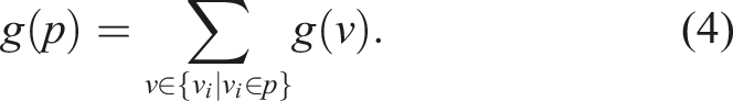
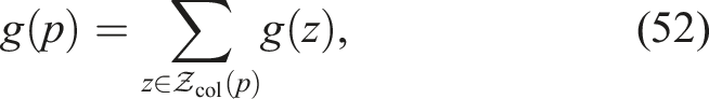
By definition, g
set
is invariant under repeated visits to the same vertex. With

An illustrative example is provided in Figure 3(a). Examples of IPP graphs. Each node has an associated gain, each edge a cost, and v
s
denotes the start node. Revisiting nodes can be advantageous. For example, the optimal solution in (b) requires multiple traversals of v3. 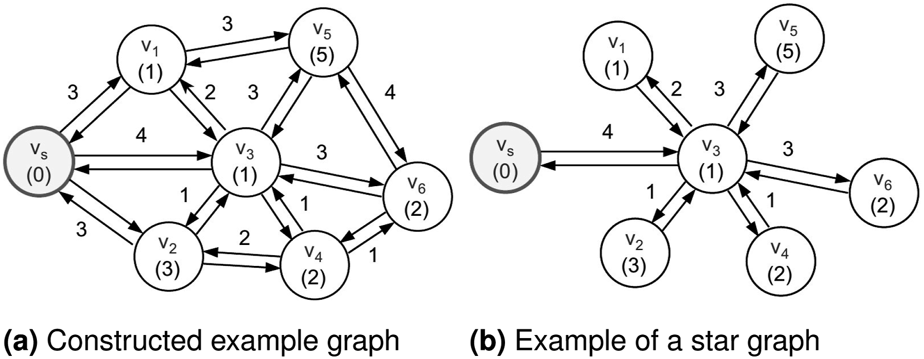
3.1. Graph a priori formulation
We first consider the case in which the environment is fully known in advance and represented as a directed simple graph as in equation (3). In this formulation, the gain accumulated along a path is computed as the sum of gains from the unique vertices visited:
Note that this complies with equation (2).
Let


The initial vertex v0 is fixed at v s , while the final vertex is unconstrained. Paths may revisit vertices and edges, which can be advantageous (see Figure 3(b), where the robot must traverse v3 multiple times to collect all gains). This formulation assumes complete a priori knowledge of the graph’s topology and associated cost and gain functions. Note that the policy π* may correspond to a one-shot plan computed at the beginning or a receding-horizon strategy that replans at every node. The notation here is general and accommodates all cases.
3.2. Graph online perception formulation
We next consider the case in which the graph is not known a priori and must be discovered incrementally through local perception. This online perception setting introduces significant challenges, particularly in balancing exploration and exploitation with partial information.
Let the environment be modeled as a directed simple graph

Let


Given a perception radius ρ > 0, cost budget C > 0, and initial vertex

This formulation reflects a setting in which the policy π* is inherently adaptive, continually updated with new local information. Note that when the perception radius ρ exceeds the graph’s diameter, the entire graph
3.3. Active perception formulation
We generalize the online perception framework to a more realistic active perception setting, where a robot operates autonomously in a continuous, bounded 3D workspace using a depth sensor with limited range, completing tasks without prior knowledge of the environment. In contrast to prior formulations that assume a directed graph as the environment, in this formulation, the robot incrementally constructs a graph as an internal abstraction solely to support planning and navigation.
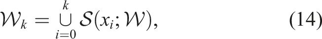
Let
The robot begins at an initial configuration


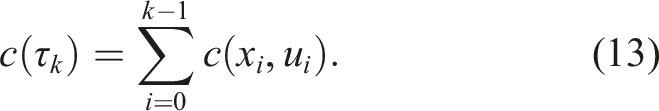
In this work, we use the term trajectory τ to denote a sequence of states and control actions generated under the robot’s velocity model with fixed timestep Δt, whereas a path p refers to an abstract sequence of vertices on a graph. Each action incurs a traversal cost
If the cost is time, then the cost is simply

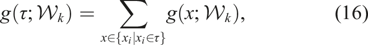
This function is sometimes instantiated as a sum over state-specific gains:
Given the sensor model


4. Preliminaries
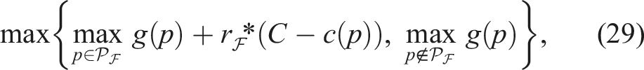
This section discusses the fundamental design choices of selection criteria and replanning strategies that underlie all subsequent algorithms for informative path planning. The choice of selection criterion is pivotal. In the graph a priori formulation (Section 3.1), the planner focuses solely on exploitation—maximizing gain within the cost constraint. In contrast, the graph online perception formulation (Section 3.2) and active perception formulation (Section 3.3) require balancing exploration (discovering new informative areas) and exploitation (maximizing collected gain). This work proposes a unified selection criterion designed to be effective across these settings. In addition, we investigate how the frequency of replanning influences performance, ranging from replanning at arbitrary frequency to single-shot planning (without replanning). Finally, we analyze the structure of optimal paths under symmetric graphs, offering insights for algorithmic design.
4.1. Selection criteria
The selection criterion defines a quality function of a path Illustration of path selection criteria. Each path is represented by a circle: open circles denote paths leading to frontier nodes 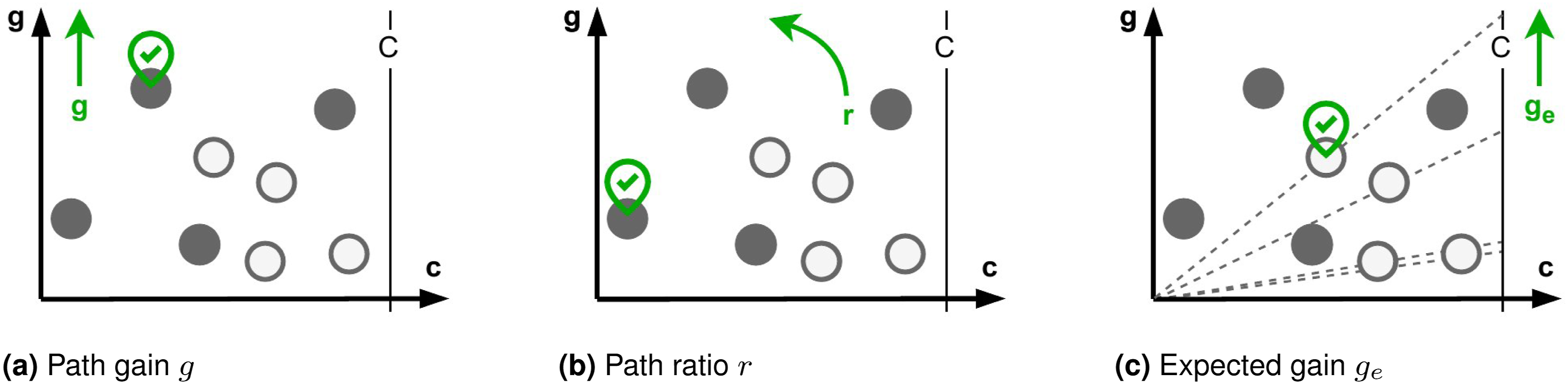
4.1.1. Path gain
The most straightforward quality function is the path gain
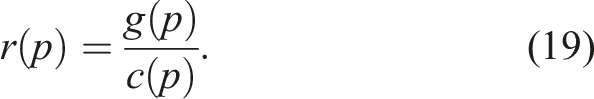
4.1.2. Path ratio/gain-to-cost ratio
Since the full environment may not be known a priori, a commonly used heuristic is to optimize for path efficiency, defined as the gain collected per unit cost:
Note that this quality function implicitly assumes that the current gain-to-cost ratio provides a reliable estimate of the future gain over the entire budget, which can be formalized as:

This ratio has been proposed as the principal objective in several informative path planning frameworks (Popović et al., 2017; Schmid et al., 2020; Xu et al., 2021). However, it does not constitute a well-defined optimization problem. Once the path with the highest ratio is identified, the robot has no incentive to continue beyond that path, as doing so would reduce the overall ratio. In contrast, practical scenarios typically impose a maximum cost budget, which should ideally be fully utilized for collecting maximum gains.
4.1.3. Expected gain
To explicitly account for exploration, we propose the expected gain, which incorporates frontier information:
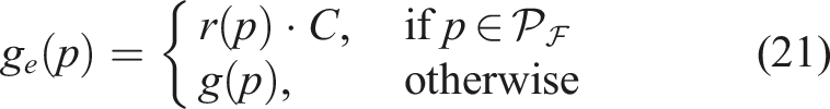
Here,
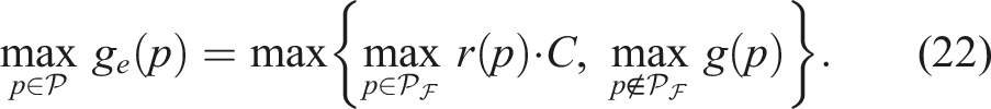
A natural question that arises is whether the extrapolation in equation (21) should use the maximum gain-to-cost ratio across all frontier paths instead of individual path-specific ratios. The following theorem establishes that both approaches yield the same path selection. Consequently, the optimal path can be determined without precomputing the maximum ratio, reducing computational overhead while preserving optimality.
Let
Proof. We prove this theorem by showing the path that achieves the highest ratio r* maximizes both path quality functions. Define, for any Let p* maximize r, meaning The term r*C is constant, so maximizing


Let
This shows that extrapolating each frontier path using its own gain-to-cost ratio yields the same optimal path as using the maximum frontier ratio
Additionally, the maximum expected gain
Notably, our formulation equation (21) allows the optimal path to be determined without explicitly computing


4.1.4. Complexity class of selection criteria
Consider the case where the path gain is defined as the sum of node gains along a path. Under this formulation, maximizing the path gain reduces to the classical longest path problem in a weighted graph, which is known to be NP-hard (Hardgrave and Nemhauser, 1962). In contrast, maximizing the gain-to-cost ratio corresponds to the maximum ratio path problem (Radzik, 2013). Ahuja et al. (1983) showed that the longest path problem can be reduced to a special case of the maximum ratio path problem. Consequently, any algorithm that solves the maximum ratio path problem can also solve the longest path problem, implying that the former is NP-hard. As the expected gain integrates both path gain and path ratio, its complexity subsumes theirs. Therefore, maximizing the expected gain is also NP-hard.
It is important to note that while the maximum ratio cycle problem is solvable in polynomial time (Dantzig et al., 1966; Lawler, 1972), this variant does not accommodate start-vertex constraints and is therefore not directly applicable to most informative path planning scenarios. That problem can be cast as detecting negative cycles (Cherkassky and Goldberg, 1999; Lawler, 1972) or solved using linear programming (Dantzig et al., 1966), but it does not generalize to the path-based formulations considered in this work.
4.2. Replanning strategies
When an underlying graph structure is available, the robot navigates by planning and executing paths over this graph. It may (i) follow a precomputed path without any replanning, (ii) replan only upon reaching the terminal node of the current path, or (iii) replan at each visited node along the trajectory, as illustrated in equations (5) and (10). In active perception scenarios, where planning and navigation are grounded in an internally constructed graph, the same three replanning strategies are applicable. Moreover, since the robot operates under velocity control, replanning can, in principle, occur at any time step. For example, the robot may execute a partial trajectory (e.g., five steps along the current path) before reevaluating its policy at an intermediate configuration. The frequency of replanning introduces a trade-off between computational cost and responsiveness to new sensory inputs.
4.2.1. No replanning
At the start node, the planner computes an optimal path

The robot then executes this plan to completion. This approach is computationally efficient but does not incorporate newly acquired information during execution and may underutilize the available cost budget.
4.2.2. Replanning at the goal
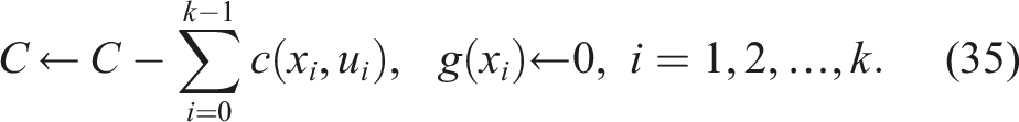
Once the robot completes the current optimal path p*, the remaining cost budget is updated, and the gain from previously visited nodes is zeroed:

The planner then computes a new optimal path based on the updated budget and updated graph. This strategy is typical in frontier-based exploration, where the robot selects the most promising frontier and replans upon reaching it (Gervet et al., 2023; Xu et al., 2021; Yamauchi, 1997).
4.2.3. Replanning at every node
Instead of executing the entire path, the robot moves to the next node v1 along edge e0,1 and then replans. The cost budget is updated, and the gain from the visited node is zeroed:

The planner then computes a new optimal path from v1. This strategy enhances adaptability to new information but incurs a higher computational cost.
4.2.4. Replanning at arbitrary frequency
In active perception settings, the robot constructs and updates its internal graph representation online, based on sensory observations. At a given configuration, the planner computes an optimal path

This strategy enables replanning at arbitrary time steps, unconstrained by discrete node transitions. Such flexibility allows for the highest replanning frequency and, consequently, the most rapid adaptation to newly acquired information, albeit at the expense of maximal computational cost.
4.3. On the structure of optimal paths
A key challenge in informative path planning is that the optimal path may revisit vertices (see Figure 3(b)), leading to an infinite number of candidate paths. However, we show that it suffices to search only for paths that do not revisit edges in a symmetric directed graph, significantly reducing the search space.
Let
Proof. Let p be a path that traverses the edge

We construct a modified path Repeated edges can be removed to construct a lower-cost path with identical gain.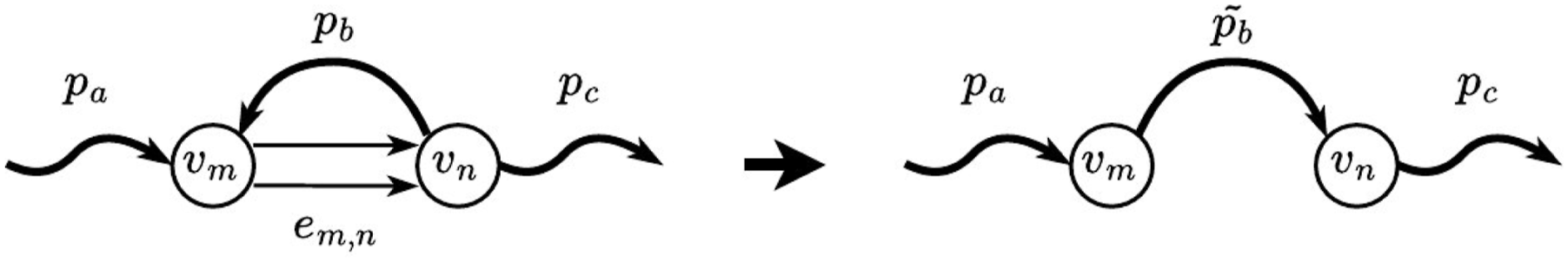

Because

By applying this transformation iteratively to each repeated edge, we progressively eliminate all edge repetitions. Although reversing a subpath may introduce new repetitions, each application strictly reduces the total number of edge traversals by two. Since the initial path is finite, the process terminates after a finite number of steps, yielding a path with no repeated edges.
Thus, any path that revisits an edge can be transformed into a trail (i.e., a path with no repeated edges) with identical gain and strictly lower cost, completing the proof. □
This theorem directly leads to the following corollary.
In informative path planning over symmetric directed graphs, it suffices to restrict the search space to
trails—that
is, paths that do not traverse any edge more than
once.
5. Informative path planning algorithms
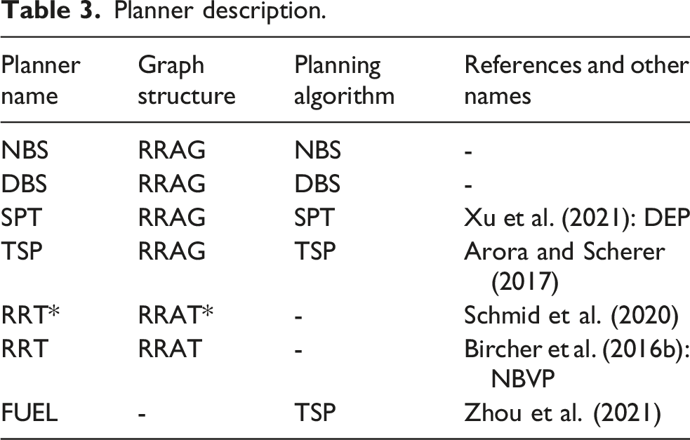
For informative path planning, we consider two widely used baseline algorithms: one based on the TSP and the other on the SPT. To overcome their limitations and improve computational efficiency, we propose beam search algorithms for solving the IPP problem. We first implement the standard beam search, referred to as depth-wise beam search (DBS), which retains the top B partial solutions at each search depth for further expansion. We then introduce a modified variant, node-wise beam search (NBS), which retains up to B candidate paths per visited node, rather than per depth level. This modification enhances the planner’s ability to explore the graph more globally and avoid becoming trapped in local optima.
To compare the potential of different paths, we define a path-preference relation that first prioritizes the gain-to-cost ratio, then the path gain, and finally penalizes higher cost when all other factors are equal.
Path Preference Relation. Let p
1
and p
2
be two candidate paths. We say that p
1
is preferred over p
2
, denoted (1) (2) (3)
5.1. Existing algorithms
5.1.1. Traveling salesman problem approach
A common foundation underlying various TSP-based approaches (Arora and Scherer, 2017; Cao et al., 2021) is a two-stage pipeline: first, a subset of nodes is sampled or selected from the full set for traversal; second, the resulting TSP instance is solved using an off-the-shelf solver. In the context of informative path planning, where the goal is to maximize information gain, the most natural strategy is to select nodes whose gain exceeds a threshold gthr. To explicitly encourage exploration, the selected set should further include frontier nodes:

The gain threshold is determined using a mid-range criterion:

Given the selected nodes from the previous stage, we first construct a cost matrix representing the shortest distances between every pair of nodes. We compute this matrix using the Floyd–Warshall algorithm (Cormen et al., 2022), which finds all-pairs shortest paths with a time complexity of
5.1.2. Shortest path tree approach
The shortest path tree approach (Xu et al., 2021) comprises two computational stages: (1) constructing the SPT, and (2) selecting the optimal path within the SPT. We employ the Bellman–Ford algorithm (Cormen et al., 2022) to compute the SPT that encodes the minimum-cost path from the source to every node. This step dominates the computational complexity, requiring
5.2. Depth-wise beam search
Beam search is a variant of breadth-first search that selectively retains the most promising partial solutions at each depth level. In the standard formulation, a fixed parameter
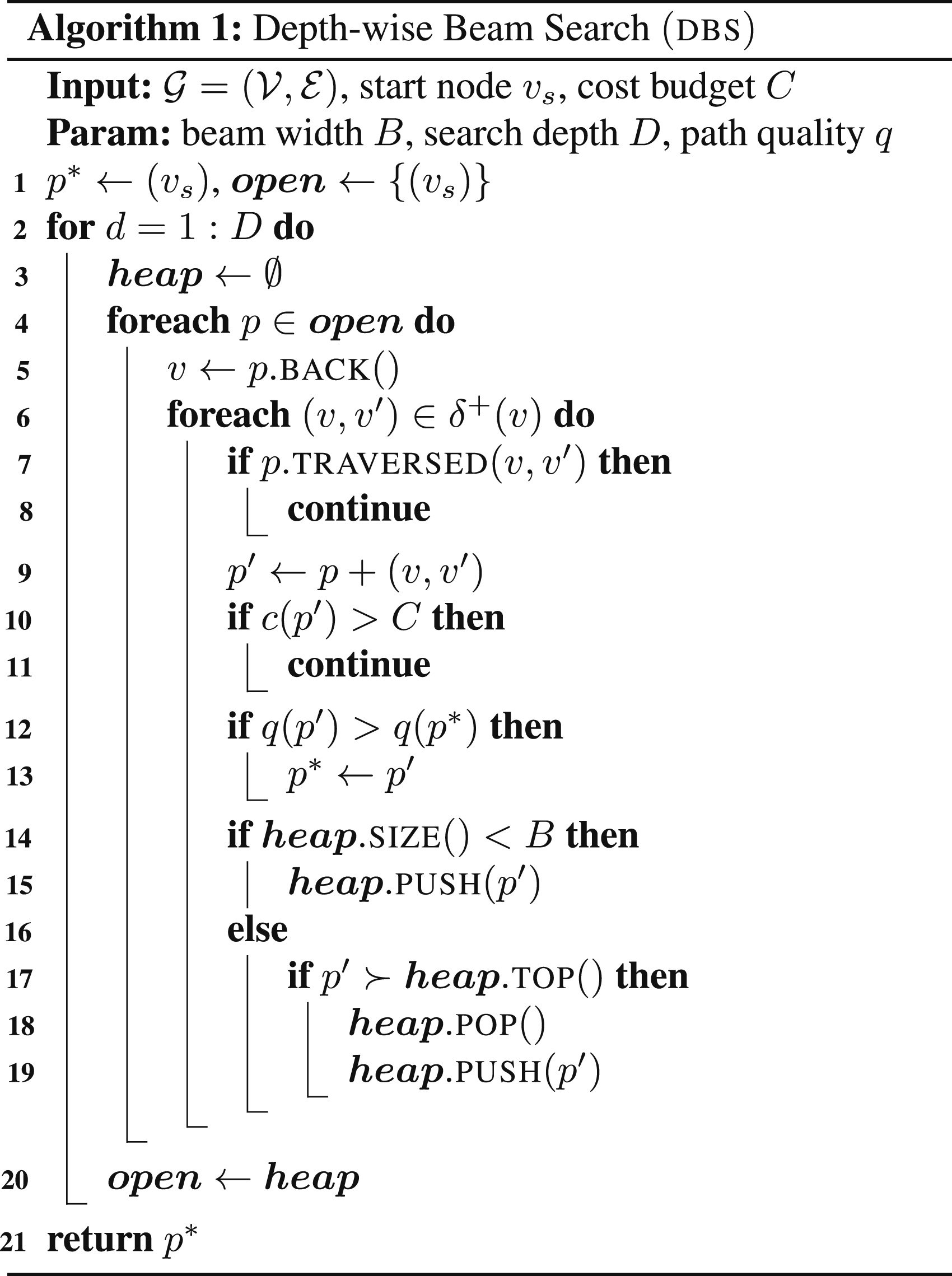
Algorithm 1 outlines the DBS procedure for identifying the most informative path in a given graph. The search begins with a beam
DBS exhibits a time complexity of
5.3. Node-wise beam search
Depth-wise beam search prioritizes expanding the most promising paths at each depth level, but this makes it easily fall prey to local optima. Once the entire beam converges on regions with high immediate gains, it will neglect other promising candidates that initially appear less favorable but could ultimately lead to better solutions. In the worst case, all paths in the beam may even terminate at the same node. To address this, we propose an alternative algorithm, NBS. Instead of maintaining the top B path candidates per depth, NBS stores up to B paths for each visited node. This modification ensures that at least one promising path remains available at every visited node, encouraging exploration across the graph rather than focusing on immediate high-gain regions.
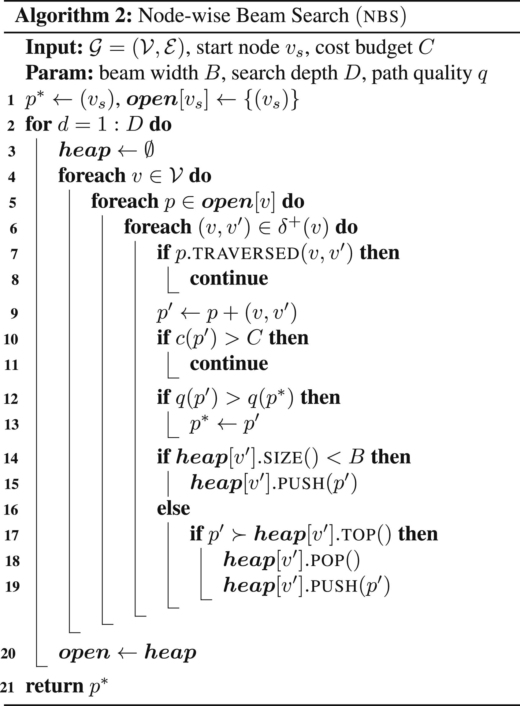
Algorithm 2 outlines the NBS procedure. The search maintains a per-node beam,
To better analyze the computational complexity, we can adjust the implementation by iterating the depth in the outer loop, then iterating over the edges
5.4. Computational complexity
Asymptotic time and space complexity of the evaluated algorithms.
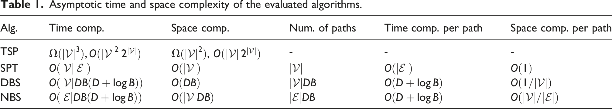
For the SPT approach, since the tree contains exactly one path to each vertex, the number of evaluated paths is
Among all methods, TSP exhibits the highest asymptotic time and space complexity with the upper bound. While direct comparison between SPT and beam search methods in terms of overall computation time is challenging due to their dependence on beam width and search depth, their per-path complexities offer clearer insight. In most scenarios, D and log B are expected to be significantly smaller than
6. Benchmarking on graphs
We evaluate all four algorithms, each with a range of key parameters. For beam search, the primary parameter is the beam width B. The maximum beam width is chosen so that DBS and NBS have comparable computation times. For DBS, the beam widths are 1, 100, and 10000; for NBS, they are 1, 10, and 100. For TSP, the relevant parameter is α, as defined in equations (40) and (41). While the shortest path tree typically does not involve tunable parameters, in Xu et al. (2021) the same parameter α is used to reduce the search space and computation time. We set α to 0.5, 0.75, and 1.0. All algorithms are implemented in C++, run in a single-threaded environment, and use the same graph representation to ensure a fair comparison. Experiments are conducted on an Intel i9-12900 CPU.
We evaluate each planner on two graph structures: clustered gains and scattered gains (examples in Figure 6). Both structures are generated at two scales: a small graph spanning 25 m in the x- and y-directions, and a large graph spanning 50 m. In the scattered scenario, vertex gains are uniformly sampled from [0,100]. In the clustered scenario, these gains are assigned only to eight randomly placed clusters (all other vertices receive zero gain). Edge costs equal Euclidean distances, with the start vertex fixed at (0, 0). For each graph type, we generate five instances and average the results for gain and computation time. Illustrations of four types of graphs used for benchmarking. 
We consider both sensing scenarios: the a priori case (Section 3.1), where the robot has full knowledge of the graph from the beginning, and online perception (Section 3.2), where the robot observes only nodes within a given perception radius ρ, gradually discovering the graph as it navigates. We evaluate all applicable pairings of selection criteria and replanning strategies. In the a priori scenario, the expected gain equals the path gain (
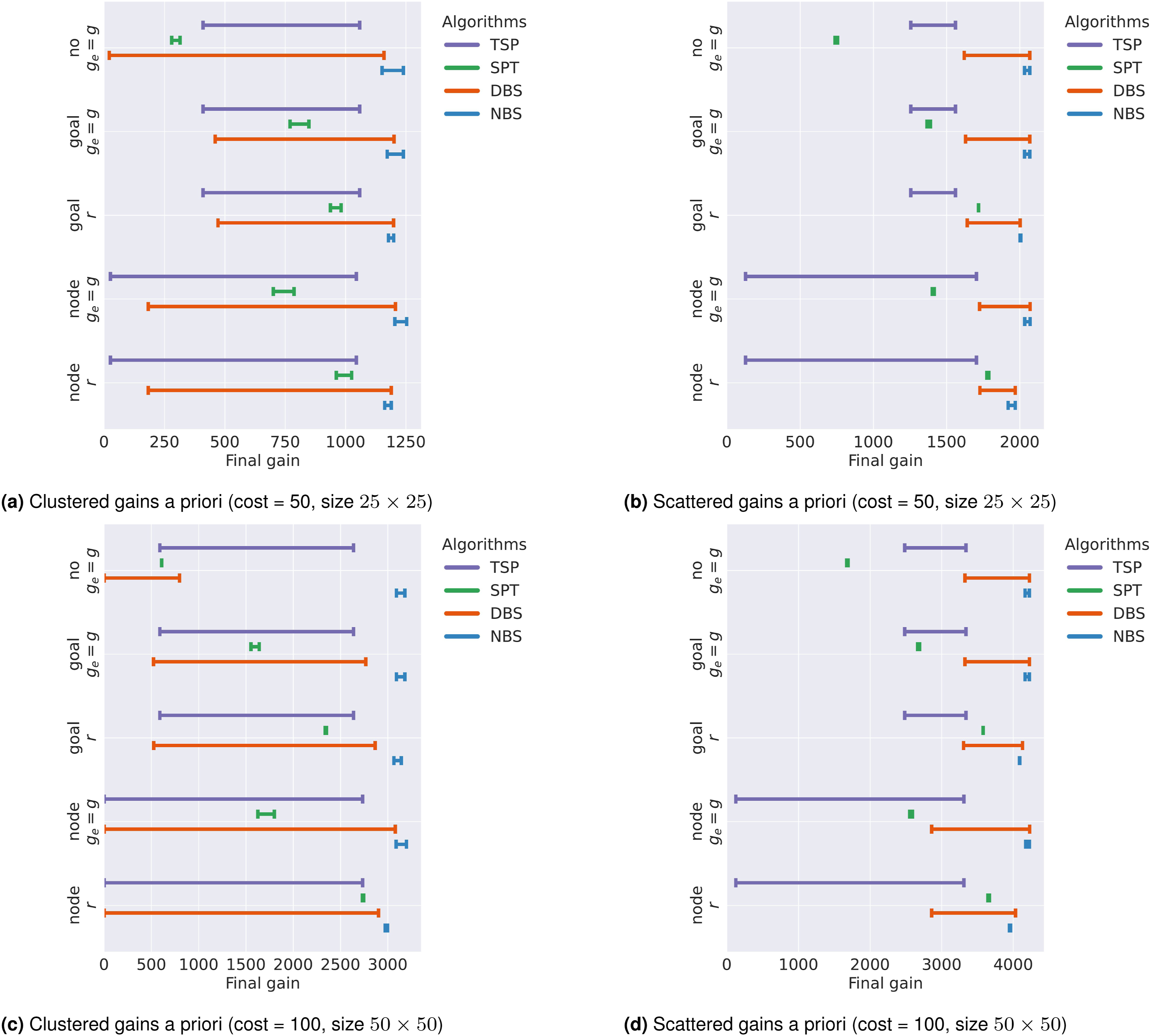
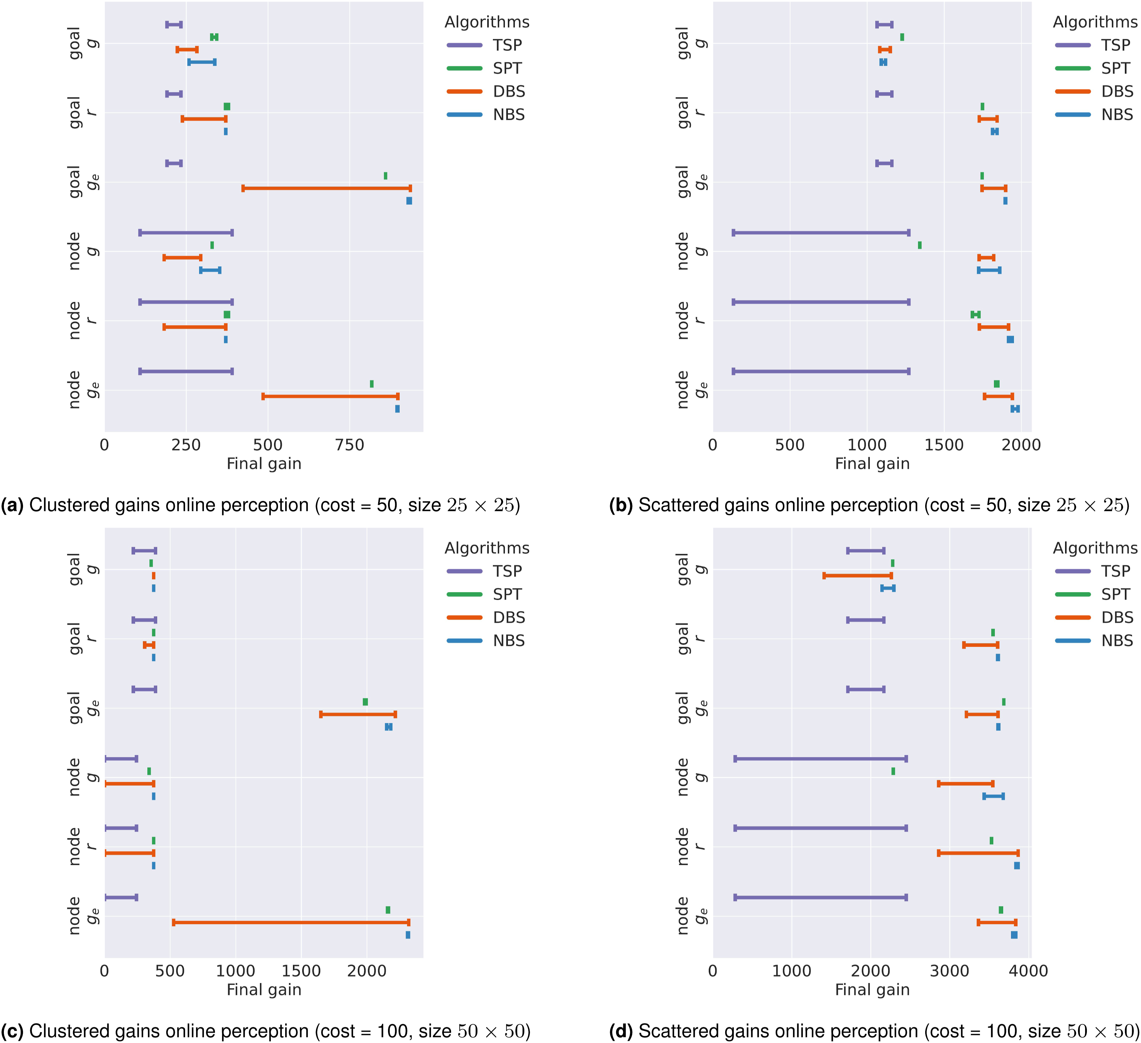
In the plots, the y-axis represents different path selection pairings, while the x-axis shows either the range of computation time or the final accumulated gain across parameter settings. Figure 7 presents the average computation time of various algorithms under different parameters. For this metric, we consider only the fully known graph case, as planning under exploration introduces significant uncertainties that can affect planning time. Figures 8 and 9 present the results for the a priori and online perception scenarios, respectively. We evaluate algorithmic performance along two principal dimensions: (i) the maximum achievable gain, represented by the rightmost extent of each horizontal bar, and (ii) sensitivity to parameter settings, indicated by the bar’s length. An algorithm is considered best if it consistently yields high gain with low sensitivity, corresponding to a short bar positioned to the far right. We prioritize the algorithm that achieves higher gain over those with merely lower sensitivity. Beyond identifying the top-performing algorithms, our analysis also aims to determine the most effective path selection combination across both formulations. Average computation time in the graph a priori experiments. The range of final collected gain in the graph a priori scenario. NBS achieves the highest and most consistent gains, as shown by short horizontal bars positioned to the far right. The range of final collected gain in the graph online perception scenario. The expected gain selection criterion delivers the strongest results overall, and replanning at every node further improves performance compared to other replanning strategies. With this setup, NBS offers the most reliable performance with little sensitivity to parameter choices. 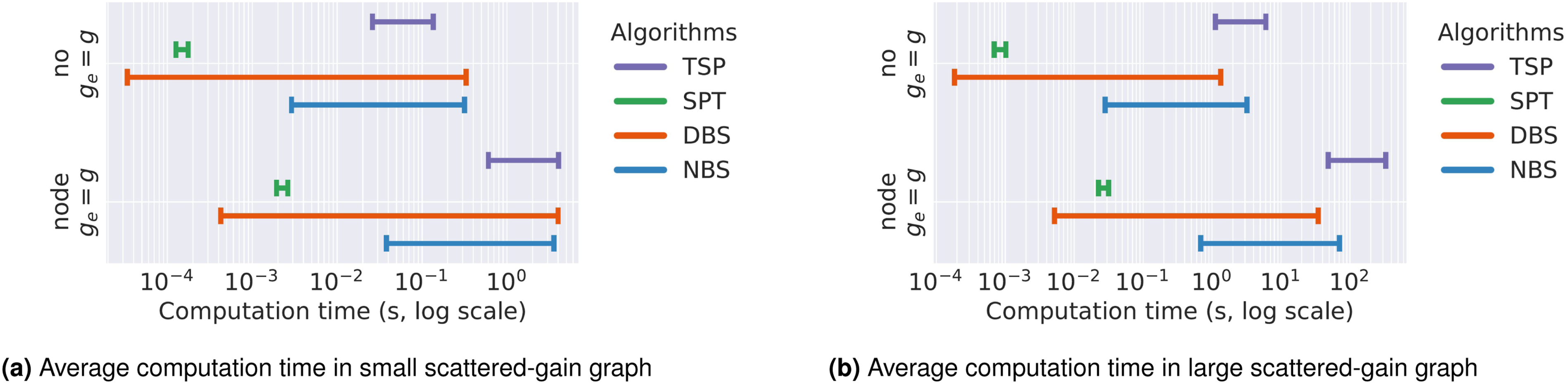
6.1. Graph a priori benchmarking
Figure 7 shows the average computation time per algorithm, in seconds, plotted on a logarithmic scale. We consider two replanning strategies: no replanning and replanning at every node; the “replan-at-goal” case is excluded due to its inconsistent replanning frequency. Results are shown only for scattered gain graphs, as clustered graphs exhibit qualitatively similar trends. We observe that computation time increases with both graph size and replanning frequency. TSP scales the worst, exceeding 300 seconds per episode on large graphs, whereas SPT remains consistently efficient. DBS achieves very low planning times at small beam widths. NBS is slightly slower than DBS at a beam width of 1, but its absolute computation time remains small: approximately 0.1 seconds for small graphs and about 1.0 second for large graphs under the every-node replanning strategy.
We visualize algorithm performance in the a priori formulation in Figure 8. NBS consistently achieves the best performance across all conditions. It exhibits low sensitivity to both parameter settings and path selection, achieving high gains—as evidenced by short horizontal bars positioned to the far right. While DBS can potentially achieve comparable gains, its performance is more sensitive to both parameter and path selection setups. For example, it performs much worse in the clustered-gain graph without replanning. Across most settings, the long horizontal bars indicate that DBS’s performance is highly dependent on careful parameter tuning. SPT is insensitive to its parameters but shows considerable sensitivity to path selection. Without replanning, SPT fails to function effectively and, overall, achieves much lower gains than DBS and NBS. TSP lacks an explicit selection criterion, and its performance varies only with the replanning strategy. It is the most sensitive algorithm: while it can occasionally match SPT’s performance, it often achieves the lowest gains due to repeatedly traversing the same edge back and forth.
Regarding path selection, the top-performing algorithm, NBS, exhibits minimal sensitivity to this choice. This suggests that the specific path selection strategy is less critical in the fully known graph scenario when a robust algorithm is employed. Consequently, we omit further discussion of path selection for this scenario.
6.2. Graph online perception benchmarking
In the online perception scenario, the robot can only perceive nodes within a fixed radius (5 m in this case). Figure 9 illustrates the algorithms’ performance with this setup. The analysis parallels that of the a priori case, focusing on maximum gain, parameter sensitivity, and the path selection combination that yields the best performance.
We observe that the expected gain objective consistently yields superior results compared to the path ratio or path gain. This advantage arises because the expected gain explicitly encourages exploration by incorporating frontier information. In contrast, the other selection criteria lack such exploratory incentives, leading planners to over-exploit known areas and become trapped in local optima. Under the expected gain criterion, replanning at every step generally outperforms replanning only at the goal. Replanning exclusively at the goal ignores new information acquired en route, resulting in suboptimal behavior in three of the four evaluated graph types.
With this path selection setup, NBS consistently achieves the best performance and exhibits low sensitivity to parameter choices. DBS can attain similar performance but is more sensitive to parameter tuning. SPT performs worse overall, limited by its tree-based structure. TSP shows the weakest performance and exhibits high sensitivity to parameter settings.
6.3. Performance analysis on graphs
The effectiveness of selection criteria depends on the underlying graph formulation. When the graph is fully known a priori, the top-performing algorithms achieve strong results across all criteria. In contrast, in the online perception setting, the expected gain consistently outperforms other criteria across all planners. Regarding replanning frequency, in the a priori case, DBS and SPT benefit significantly from frequent replanning to improve performance. While TSP can also benefit from higher replanning frequency, it often exhibits oscillatory behavior between competing paths. Notably, NBS maintains strong performance across all replanning frequencies (even without any replanning), highlighting its robustness and computational efficiency. In the online perception setting, when paired with the expected gain criterion, high-frequency replanning mostly improves gain accumulation. This combination enables planners to effectively balance exploration and exploitation, adapting in real time to newly acquired information.
NBS demonstrates exceptional robustness to parameter variations, enabling reliable deployment with minimal tuning effort. Even at the smallest beam width (B = 1), it delivers strong performance. In contrast, DBS is more sensitive to beam width selection—poor parameter choices can significantly degrade its performance. SPT remains the most computationally efficient but sacrifices solution quality due to its restricted search space. TSP performs poorly overall: it is highly sensitive to its parameters, prone to oscillations between suboptimal paths, and exhibits poor scalability, with prohibitively high computation times on larger graphs.
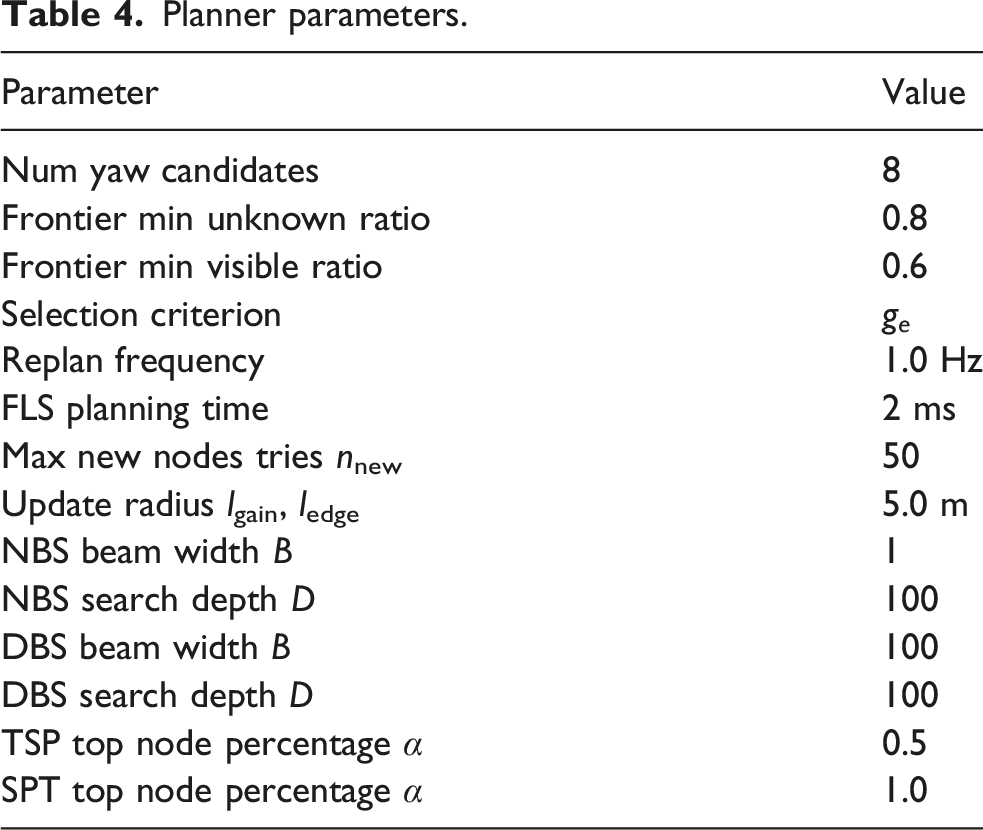
Overall, our results show that NBS is the top-performing IPP algorithm. The combination of the expected gain metric with every-node replanning demonstrates the most effective selection strategy. Together, they form the best-performing planning approach, consistently achieving superior results in both a priori and online perception scenarios. In the following section, we shift our focus to active perception. Based on our findings, we adopt the expected gain criterion and apply a high replanning frequency. NBS is selected with a beam width of 1, as it is the most robust and reliable algorithm across all settings. DBS is configured with a larger beam width (B = 100). For SPT, given its computational efficiency, we evaluate the entire tree search space by setting the threshold α to 1.0. The TSP algorithm is configured with a threshold of 0.5.
7. Graph construction for active perception
As introduced in Section 3.3 and illustrated in Figure 2, active perception does not assume a predefined underlying graph environment, unlike prior IPP problems defined on graphs. Therefore, to apply IPP algorithms, we incrementally build a graph as the robot explores the environment.
Following prior work (Schmid et al., 2020; Xu et al., 2021), we enforce a minimum edge length constraint lmin: a newly sampled, collision-free configuration is accepted only if its distance to all existing graph nodes exceeds lmin. This helps avoid oversampling that would yield highly redundant information and improves computational efficiency during information-gain evaluation and path planning. Once accepted, bidirectional edges are attempted between the new node and its neighbors, subject to a maximum edge length lmax and the existence of a collision-free path. The maximum edge length prevents excessive edge density, such as
The resulting structure, in which edges exist only between nodes separated by distances within the interval [lmin, lmax], is known as an annulus graph (Lichev and Mihaylov, 2024). In such graphs, the number of outgoing edges per node—referred to as the out-degree—is inherently bounded. This bound follows from a geometric sphere-packing argument: specifically, the maximum number of non-overlapping spheres of radius 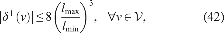
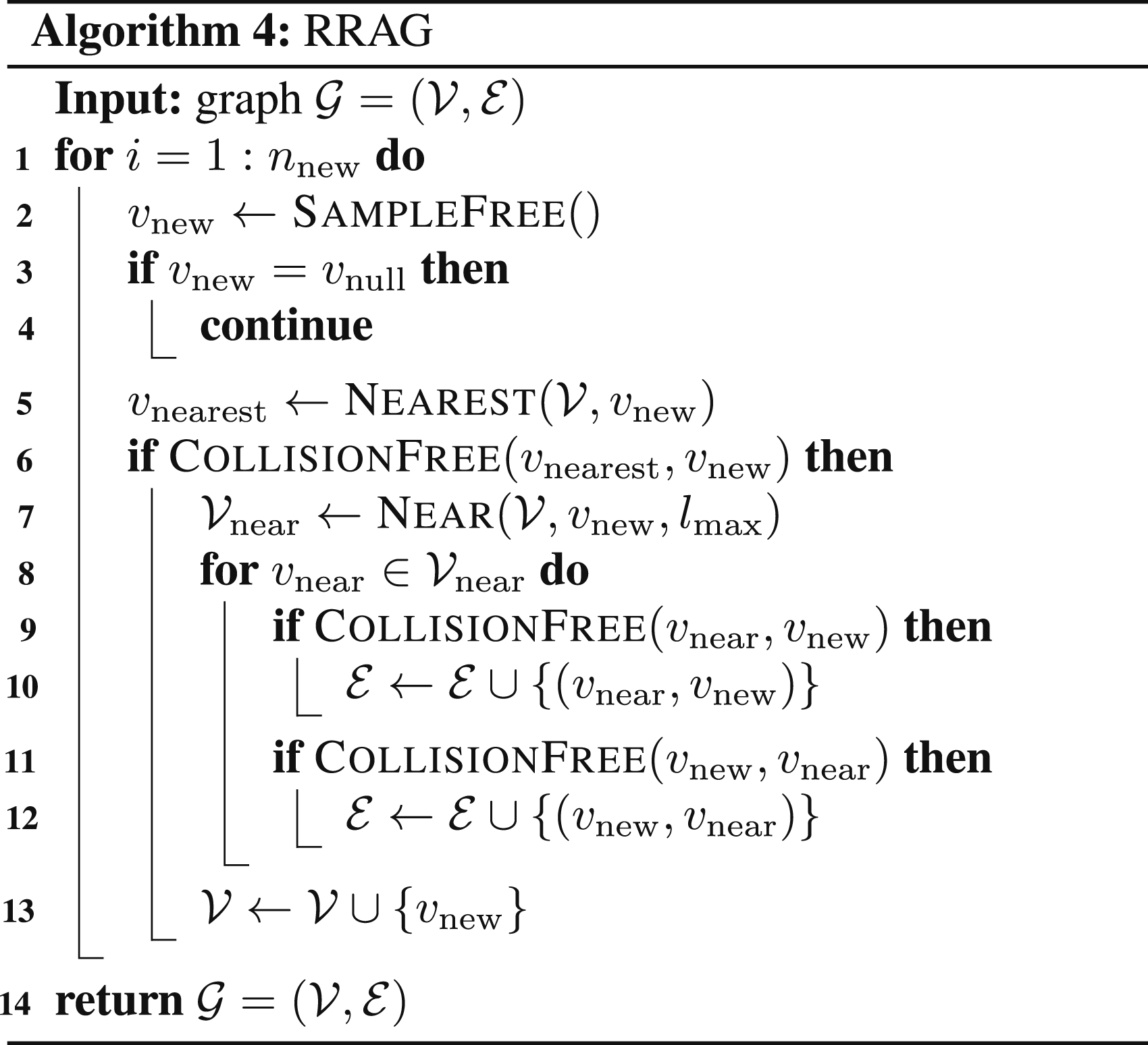
We introduce the rapidly-exploring random annulus graph (RRAG), a variant of the RRG that incorporates both minimum and maximum edge length constraints. The graph construction procedure is described in Algorithm 4. The auxiliary function
7.1. Collision checking between nodes
To determine whether a trajectory between two nodes is feasible, we must verify that it lies entirely within the free space
When connecting two configurations via straight-line interpolation in
Path length bound (Barraquand et al., 1997). For any bounded robot, there exists a constant η > 0, such that when the robot moves along the straight-line path between any two configurations x1 and x2, every point on the robot traces a curve of length at most η‖x1 − x2‖2 in the workspace.
This bound allows us to derive a sufficient condition under which linear interpolation between two collision-free configurations remains entirely within
Adjacency (Barraquand et al., 1997). For a self-collision-free robot, two configurations 
If self- collisions are possible, the right- hand side should be scaled by 1/ 2.
This sufficient condition leads to the following guarantee for collision-free edges in annulus graphs.
For robots without self-collision risks, any attempted trajectory verification in RRAG between
Proof. In RRAG, edges are only formed between nodes satisfying ‖x1 − x2‖2 ≤ lmax. To ensure that the linear path lies entirely in 
Requiring
Similarly, when ‖x1 − x2‖2 = lmin, we require
Imposing
Therefore, in narrow or heavily cluttered workspaces, where clearances are typically small, lmin and lmax must be reduced accordingly to guarantee sufficient graph coverage. However, this adjustment results in a denser graph, leading to highly overlapping information gains and significantly increased computational burden. If not properly tuned, the robot may fail to establish new edges, stalling graph expansion. To address this, we introduce a fallback local sampling-based planner (FLS) to recover valid transitions in cluttered or geometrically complex regions where straight-line interpolation would otherwise fail, as illustrated in Figure 10. The FLS is integrated into all three graph construction methods (RRAG, RRAT, RRAT*). Specifically, we employ the standard RRT* algorithm, implemented via the OMPL library (Sucan et al., 2012), to explore alternative collision-free paths locally. The FLS operates within an axis-aligned bounding box that tightly encloses the start and goal configurations, expanded by a margin of lmax in each dimension. It is invoked with a planning time budget to minimize path length. Thanks to the probabilistic completeness of RRT*, the planner will eventually find a valid path if one exists, given sufficient time. The necessity of the FLS in narrow passages. The FLS can find a path through a narrow “L”-shaped corridor when a straight-line connection fails.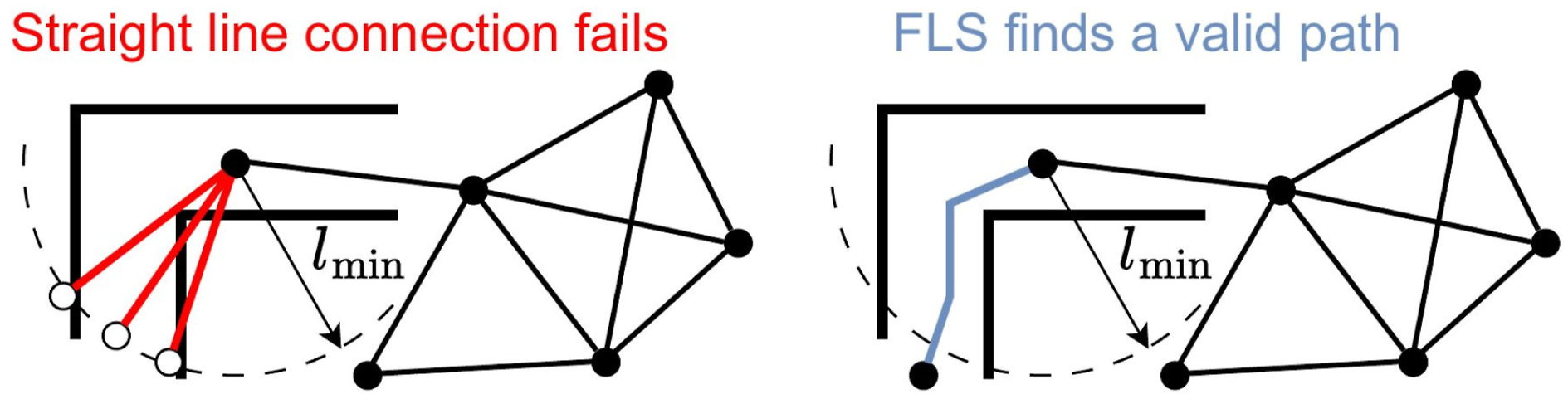
7.2. Connectivity of annulus graph
While Galhotra et al. (2019) provided initial theoretical insights into the connectivity of random annulus graphs, their analysis primarily focuses on point sets sampled on a unit sphere (e.g.,
Let
(1) l
min
-packing: Nodes in (2) l
min
-covering: Every point in
Let

Proof. We first prove the sufficiency condition by contradiction. Suppose lmax ≥ 2lmin, but
Since
By the lmin-covering property, 
Define the covered regions:
At this boundary point, there exist nodes 
Given lmax ≥ 2lmin, it follows that
For necessity, consider a counterexample in one dimension. Let
However, ‖0 − d‖ = d > lmax, so no edge exists between the two nodes. Thus,
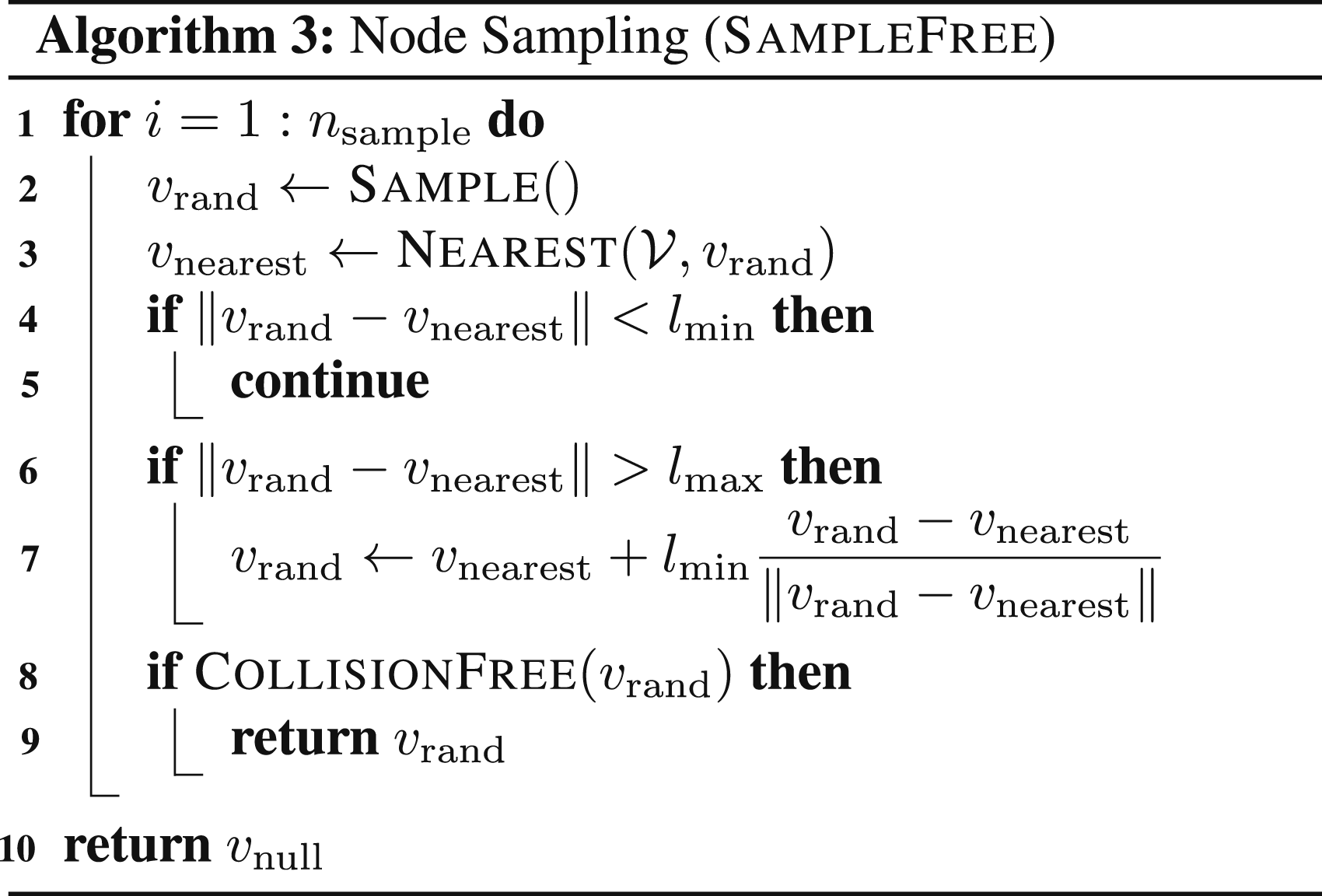
Theorem 4 requires two conditions. The packing condition is inherently enforced by our sampling procedure (Algorithm 3), which rejects any new sample within distance lmin of existing nodes. The covering condition means that the vertices must be sufficiently densely sampled to ensure effective coverage of the free space, which encourages using a sufficiently large nnew in Algorithm 4.
7.3. Preserving all orientations
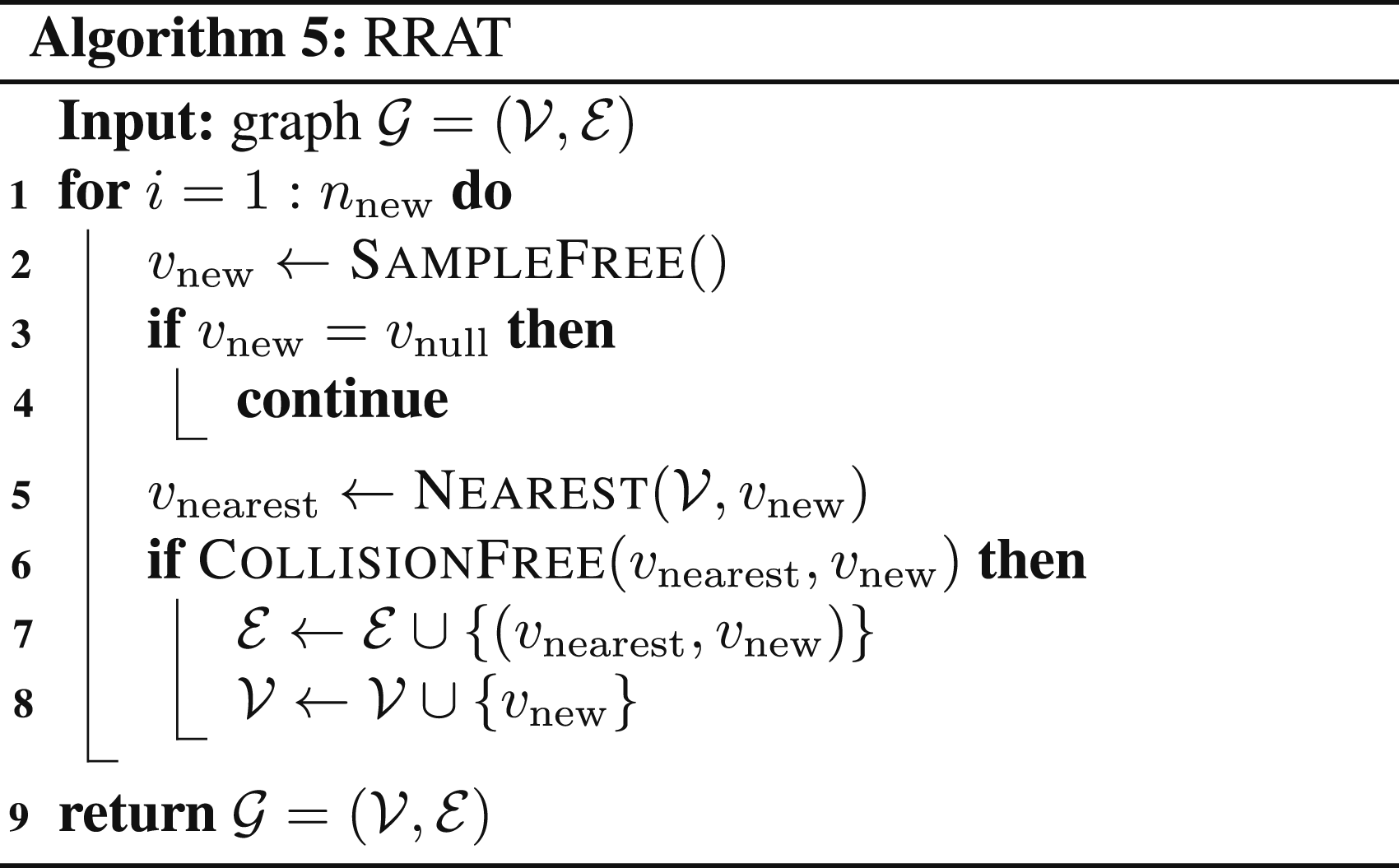
In prior work, orientation is typically managed by discretizing the yaw space and selecting a single orientation per sampled position based on the highest gain, while discarding all other candidates (Schmid et al., 2020; Witting et al., 2018; Xu et al., 2021). Consequently, once a node is selected by the planner, its assigned orientation must be reached through additional turning—even if such rotation is less advantageous than proceeding directly to other nodes. Both RRAT and RRAT* adhere to this strategy.
In contrast, our graph representation provides greater flexibility. For each sampled position, all discrete orientations are retained and treated as distinct nodes. The set of nodes corresponding to different orientations at the same position is referred to as a node cluster. Within each cluster, adjacent orientation nodes are connected by bidirectional edges, provided the transitions are feasible. For connections between different clusters (i.e., inter-cluster edges), connectivity is simplified by retaining only two directed edges (one in each direction) rather than creating a fully connected graph. These edges are constructed by selecting, in each cluster, the node whose orientation is most aligned with the direction of traversal, thereby minimizing unnecessary reorientation during inter-cluster motion. An example of RRAG with all orientations preserved is shown in Figure 11. Example of the RRAG with all orientations preserved. Only the edges are visualized. An offset perpendicular to the edge direction is applied to inter-cluster edges to distinguish overlapping connections. For intra-cluster edges, an offset is applied along the node’s yaw direction, forming a polygonal pattern around the actual node. Since FLS can be used to connect nodes, the edges are not strictly straight lines.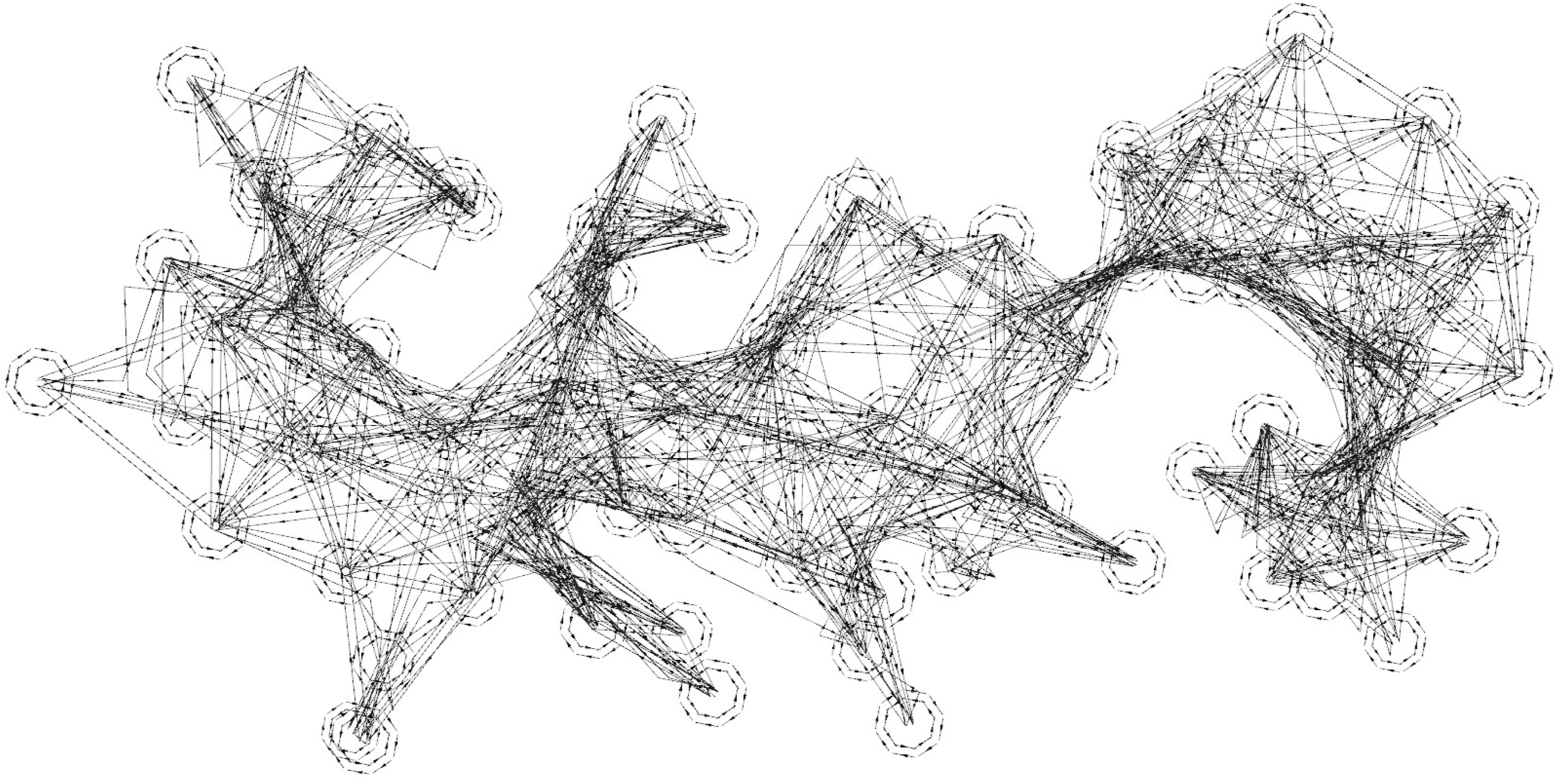
7.4. Graph updating
Prior to each replanning step, the planner updates both node gains and the graph structure. Node gains are recomputed within a local neighborhood of radius lgain centered at the robot’s current position. For RRAT and RRAT*, the best yaw is reselected at each update. Graph structure updates are handled differently depending on the planner. In all cases, edges are revalidated within a local region of radius ledge; any edge that no longer satisfies feasibility constraints is removed. For RRAT, graph updating further includes pruning all child edges of the current root node except the one selected for traversal. For RRAT*, there is a rewiring mechanism that rewires all nodes in the tree relative to the new root. While effective, this step is computationally expensive due to the need for collision checks across numerous node pairs. In contrast, RRAG benefits from its graph structure: since edges are not constrained to form a tree, no additional rewiring is required during replanning. After edge revalidation, the graph expansion process continues as in Algorithms 4, 5, and 6.
Different planners handle replanning slightly differently. For RRAT and RRAT*, which maintain a strict tree structure, this is done by introducing an intermediate node at which replanning is triggered, and then splitting the current edge at this intermediate node. Once the robot reaches this intermediate node, replanning proceeds as discussed, including gain updates, edge revalidation, graph expansion, and path selection. In the RRAG setting, the original edge is retained, and two new edges are added—connecting the start of the current edge to the intermediate node, and the intermediate node to the end of the current edge. Additionally, RRAG attempts to connect the intermediate node to nearby nodes within distance lmax via outgoing edges, enabling the robot to consider alternative paths beyond the original trajectory. The intermediate node is discarded once the robot reaches the next node.
8. Experiments on active perception
To evaluate the proposed planner, we conduct experiments in a simulated environment using Habitat (Savva et al., 2019) with the HSSD dataset (Khanna et al., 2024), a synthetic collection of diverse 3D environments. We consider eight distinct scenarios, which are visualized along with their IDs in Figure 12. Eight HSSD scenarios used in the active perception simulation environment. Note that the scenarios are displayed at different scales for visualization purposes.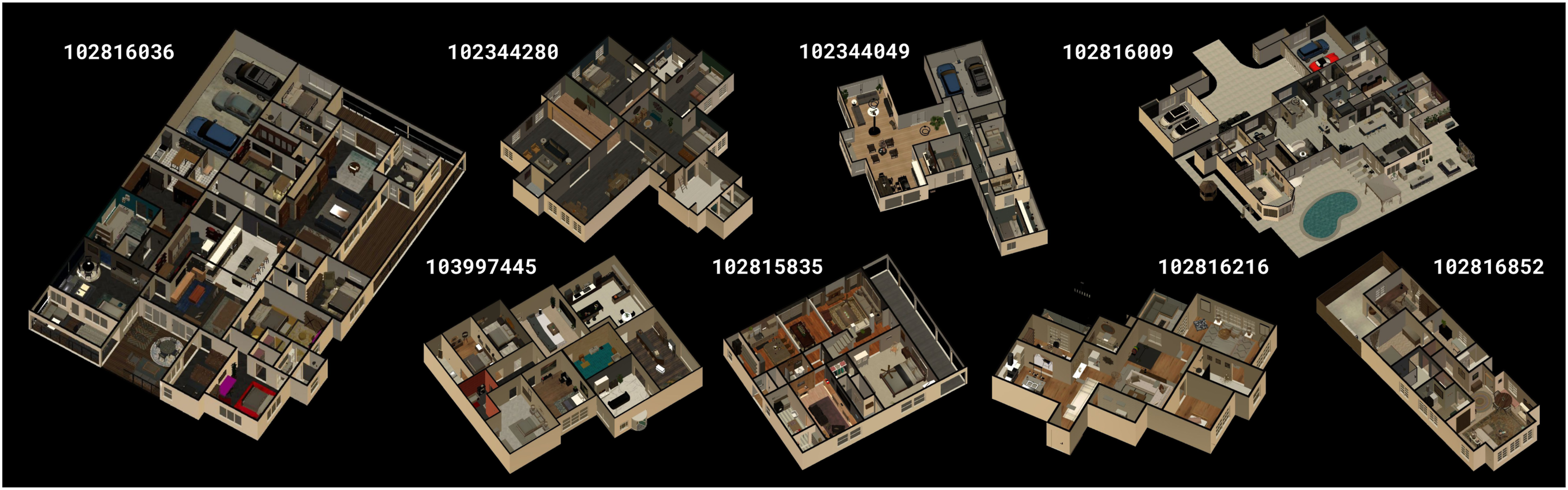
Robot parameters.
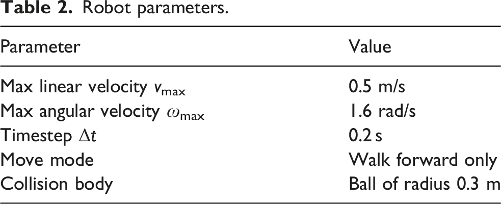
We consider three representative application scenarios: (i) point collection in an observed area, (ii) surface mapping for 3D reconstruction, and (iii) volumetric exploration. These tasks differ primarily in their respective gain definitions. In the point collection scenario, gain is computed by identifying all observed points within a local neighborhood of each node. The total path gain is defined as the sum of all unique points near the nodes visited along the path. For surface reconstruction, we adopt the surface frontier criterion introduced by Yoder and Scherer (2016). In the volumetric exploration setting, gain corresponds to the number of unknown voxels within the sensor’s field of view. For both surface reconstruction and volumetric exploration, inter-node gain correlations are neglected; node-level gains are simply aggregated along the trajectory, following established practice (Schmid et al., 2020; Witting et al., 2018; Xu et al., 2021).
We further analyze the relationship between the modeled gain g and the realized gain f (the principal objective). In the point collection scenario, the gain estimate is exact, as it accounts for all visible points and captures spatial correlations. For surface reconstruction, the estimate is conservative and constitutes a lower bound, as the surface frontier only considers unknown voxels adjacent to occupied regions as potential surface continuations. In contrast, the volumetric exploration model provides an upper bound, assuming visibility through free space while ignoring occlusions. By evaluating different algorithms under these differing modeling assumptions, we aim to demonstrate the robustness and effectiveness of our proposed algorithm.
Planner description.
Planner parameters.
The remainder of this section details each application scenario and presents corresponding benchmarking results. We then discuss validation of the pipeline on a physical robot platform using onboard computation.
8.1. Point collection
In the point collection scenario, the robot observes a set of collectible points and must navigate to within a Euclidean distance lcol of each point (orientation-independent) to collect it. Let 
Because the collection neighborhoods of different nodes may overlap, we impose a non-redundancy constraint: once a point z is collected (i.e., its gain has been accounted for), any future visit to nodes within distance lcol of z yields no additional reward. Formally, for a path 
This setup parallels the object-goal navigation (Batra et al., 2020) task, albeit without relying on semantic mapping. The core mechanism is similar: after observing a target, the robot must navigate to its vicinity to realize the reward. Consequently, the robot must balance exploration of unobserved regions against exploitation of known collectibles. An example of an agent collecting points is visualized in Figure 13. For evaluation, points are uniformly sampled within the bounding volume and assigned integer gains g(z) ∈ [0, 10], with both positions and gains held constant for all algorithms to ensure fair comparison. The collection radius lcol is set to 1 m, as in the Habitat ObjectNav Challenge (Yadav et al., 2023). Accordingly, we set the minimum and maximum distance thresholds to lmin = 1 m and lmax = 2 m, respectively. Visualization of an agent navigating to collect points represented as golden rings. These points are initially unknown and become visible only when the corresponding regions are perceived by the agent. The trajectory is visualized using a temporal gradient, transitioning from dark blue (start) to bright yellow (end). Each node is visualized as an arrow, with clusters of nodes at identical positions forming node clusters. Node gains are color-coded, with blue indicating the lowest gain and red the highest. Frontier nodes are emphasized with larger markers, while transparent nodes indicate non-frontier nodes with zero gain.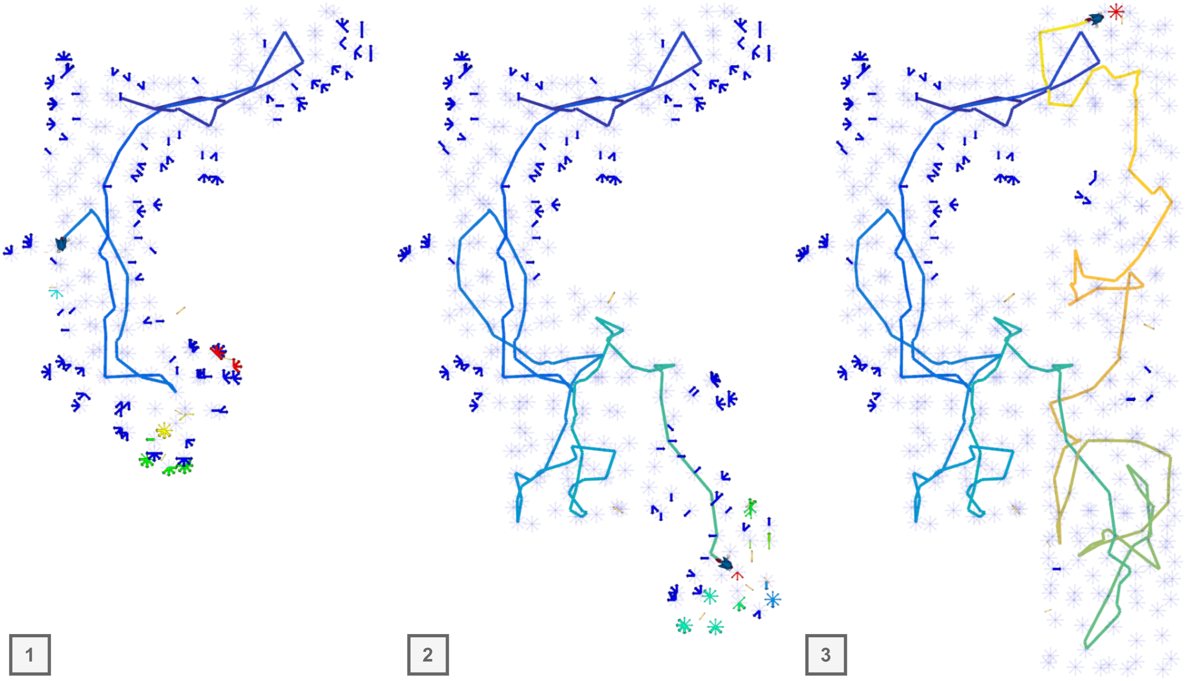
8.2. Surface reconstruction
In surface reconstruction, the objective is to scan and recover the geometry of a scene as completely as possible, quantified by the total number of voxels ultimately classified as occupied. However, this true objective f, as used in equation (18), cannot be directly computed because it requires complete knowledge of the environment—information unavailable to the robot during exploration.
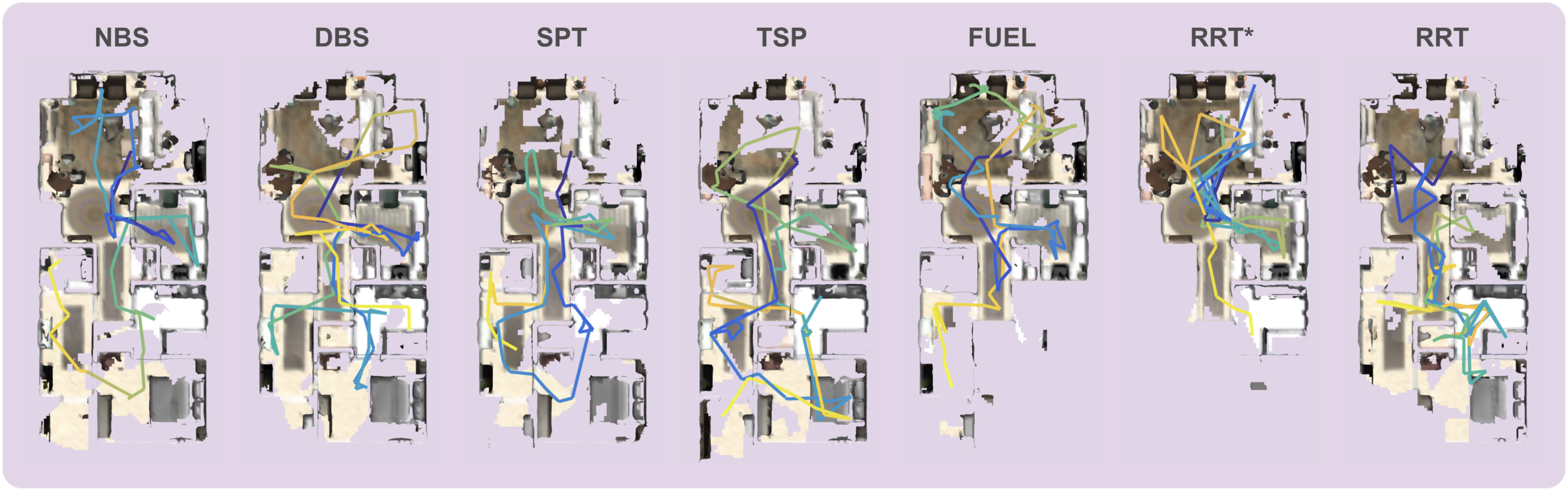
Therefore, we define our gain function g in equation (15) using the concept of surface frontiers (Yoder and Scherer, 2016). Surface frontiers are unknown voxels that are adjacent to currently known occupied voxels (i.e., the reconstructed surface). For each node v, the gain is calculated as the number of such frontier voxels visible from v: Qualitative comparison of surface reconstruction for scene 102816852. Each planner is executed 10 times, and the visualization shows the worst-case result among the trials, representing a lower-bound performance. The total reconstructed surface area (in square meters) for each planner is as follows: NBS: 445.73, DBS: 419.10, SPT: 349.96, TSP: 432.21, FUEL: 341.03, RRT*: 301.75, and RRT: 348.43. The trajectory is visualized using a temporal gradient, from dark blue to bright yellow.
8.3. Volumetric exploration
In the task of volumetric exploration, the objective is to observe as much of the unknown environment as possible, which can be measured by the total number of voxels whose occupancy state is known after the exploration. This includes both free and occupied voxels that have been successfully classified. Unlike other tasks, volumetric exploration directly equates gain collection with exploration itself. Thus, there is no intrinsic need to trade-off between exploration and exploitation.
As with surface reconstruction, the true objective f is not accessible during execution. Therefore, the gain g at each node is defined as the number of unknown voxels visible from that node, a commonly used metric due to its simplicity and practical effectiveness. Formally, for any node v, the gain is given by:
Following the setup for surface reconstruction, we set lmin = 1.5 m and lmax = 3 m, and compute the total gain along a trajectory as the sum of node gains.
8.4. Performance analysis in active perception
Each algorithm is evaluated across the three application scenarios over 10 independent trials, with execution terminated upon reaching a predefined maximum planning time. The resulting performance curves, showing average gain as a function of cost, are presented in Figure 15 for five large environments and Figure 16 for three small environments. For each curve, the mean and standard deviation of accumulated gains are calculated from linearly interpolated gain values over a cost range from 0.0 to the smallest final cost achieved by the corresponding algorithm. The mean and half the standard deviation of accumulated gain across large HSSD scenarios. Trajectory time serves as the cost function with a 10-min budget. Planning terminates at the 15-min time limit. The mean and half the standard deviation of accumulated gain across small HSSD scenarios. Trajectory time serves as the cost function with a 5-min budget. Planning terminates at the 7-min time limit.
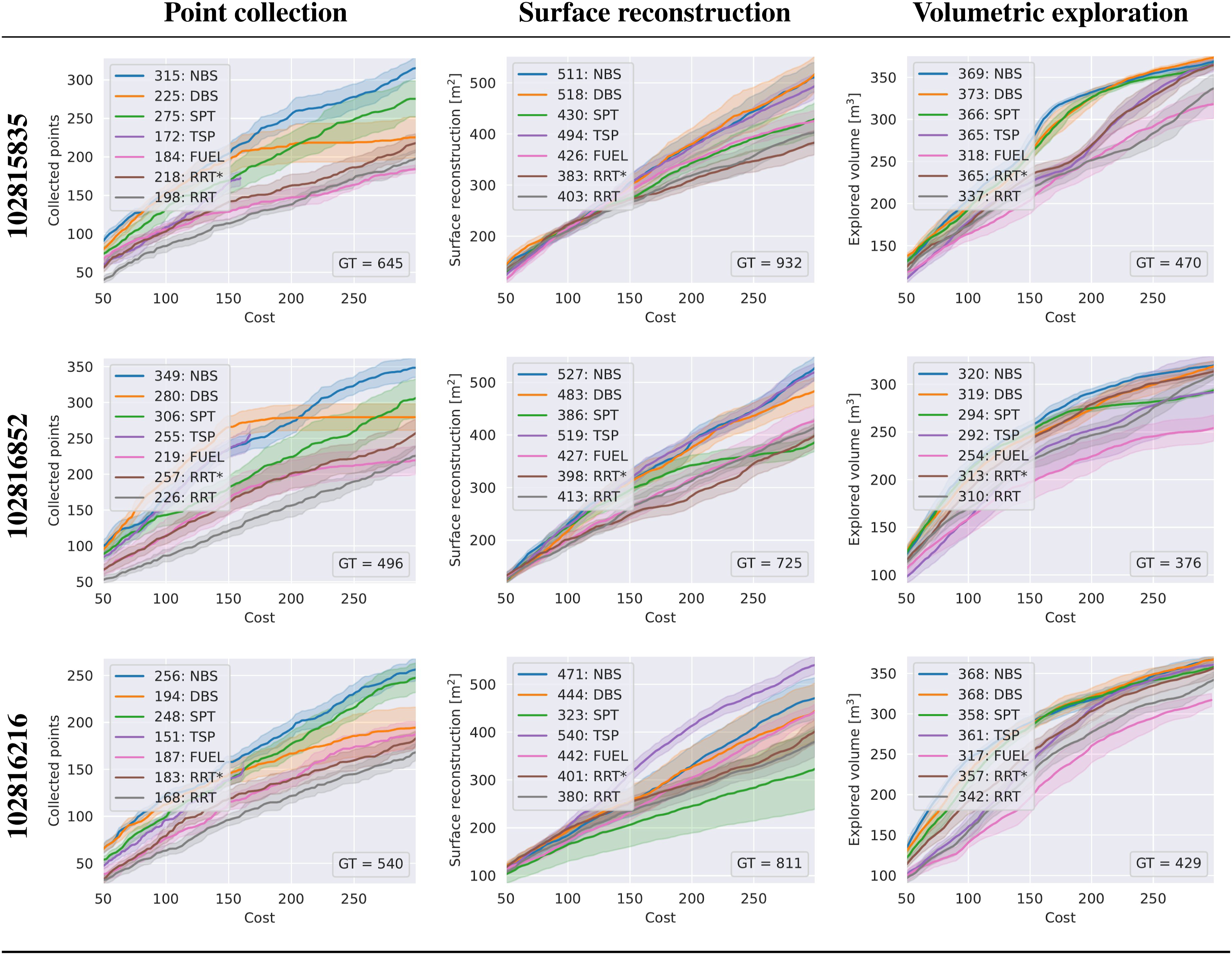
Since gain varies across environments and tasks, we use normalized gain to enable comparisons across different scenarios (Figure 17). For each task and environment, we run both NBS and RRT twice for a sufficient duration until the gain plateaus. We take the maximum observed gain from these four runs as an estimate of the ground truth (see Figures 15 and 16) and normalize the gain with respect to this value. Comparison of normalized gain across methods and tasks.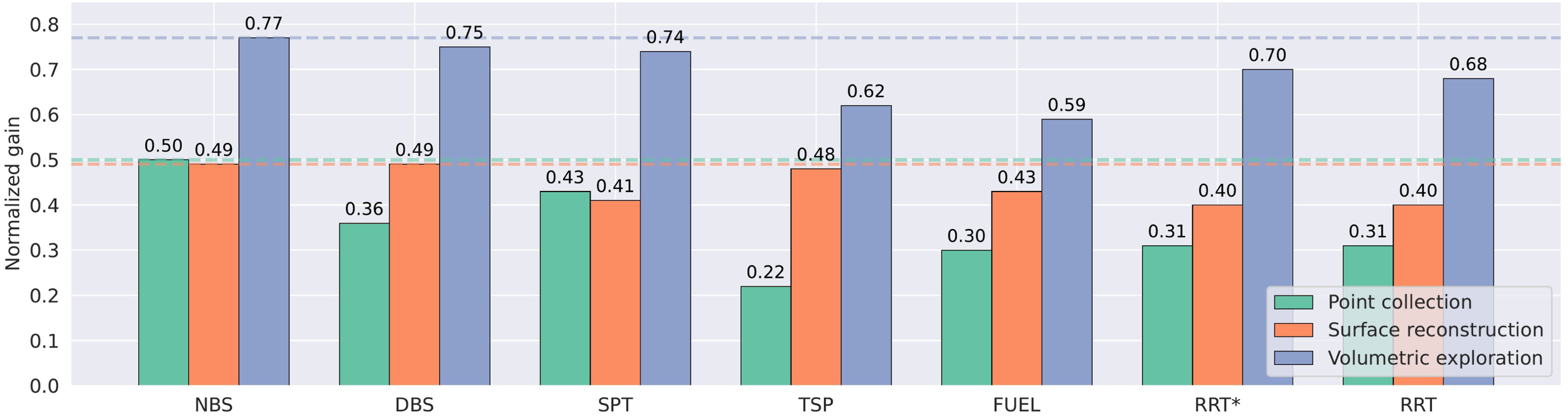
The three tasks present different levels of difficulty. Exploration is the easiest, as all algorithms achieve more than 0.50 normalized gain. This is intuitive, since this task does not require the robot to exploit the known environment. The other two tasks are more challenging, as they require a balance between exploration and exploitation. Surface reconstruction has a medium level of difficulty, with the worst performance around 0.40. Point collection is the hardest, due to the smaller collection radius and consequently denser graph. The worst-performing algorithm achieves only 0.22 normalized gain.
NBS achieves the highest performance across all three tasks: 0.50 in point collection, 0.49 in surface reconstruction, and 0.77 in exploration. Moreover, NBS outperforms other algorithms by at least 20% in one or more tasks, highlighting its robustness and effectiveness. In point collection, it demonstrates a significant improvement, surpassing the second-best algorithm by 16% (increasing normalized gain from 0.43 to 0.50).
DBS performs best in surface reconstruction, primarily because this task often requires the robot to thoroughly map its immediate surroundings before exploring farther. In such cases, DBS’s preference for locally optimal paths becomes an advantage. However, it performs notably worse in point collection. This degradation arises from the sparser gain distribution in this setting, where DBS is prone to getting trapped in local regions with low or zero gains. This behavior reveals a fundamental limitation of DBS: its susceptibility to local optima.
SPT underperforms relative to NBS, primarily due to its constrained search space. The performance gap is particularly pronounced in point collection and surface reconstruction, where the limited candidate set often yields trajectories biased toward either exploration or exploitation, without effectively balancing the two.
RRT* exhibits similar limitations, further exacerbated by the need to rewire the tree when the root node changes, which incurs significant computational overhead. Moreover, it lacks full orientation coverage, often requiring inefficient back-and-forth maneuvers to execute simple turns. RRT inherits some of these drawbacks: although computationally efficient, its continuous node pruning and sparse graph structure can lead to suboptimal decisions.
The TSP algorithm should, in principle, be well-suited for surface reconstruction, as TSP tends to prioritize high-gain nodes in the vicinity before expanding to other regions. However, we find that it suffers from excessive computational demands. In practice, it often fails to complete within the allotted time budget, resulting in the lowest average performance among the evaluated methods. Additionally, its performance is even worse in the other two tasks, as the decoupling of node selection and path optimization can lead to poor node choices that the TSP is then forced to traverse.
In contrast, the FUEL planner is driven by frontier information and generates a relatively sparse set of viewpoints to traverse, contributing to its time efficiency. Its overall performance trend closely resembles that of the other TSP-based planner. However, FUEL performs poorly on the point collection task, as this requires specific point-level information rather than just frontier awareness. Because FUEL actively maps all frontiers, it tends to exploit nearby viewpoints before moving to distant regions, leading to comparatively better performance in surface reconstruction than in pure exploration. Since the robot assigns only one viewpoint per location, it would need to travel back and forth to perform simple turns, which could consume the cost budget compared to our approach.
8.5. Hardware experiments
We deploy our planner on the ANYmal quadruped robot (Hutter et al., 2016), equipped with a ZED X Mini camera mounted on the front-facing end-effector, offering a field of view of [74°, 45°]. On the physical platform, depth estimation from a ZED X camera is processed onboard by an NVIDIA Jetson Orin, while the mapping and planning modules execute on an Intel Core i7 CPU. Captured RGB-D images are converted into colorized, downsampled point clouds, which are subsequently used by Voxblox for volumetric map generation. Unlike the simulation setup, the real-world deployment constrains the planner to a two-dimensional search space at a fixed height. The collision model is adapted to better encapsulate the legged robot’s body, resulting in larger and additional collision spheres. Consequently, collision checking needs to be more optimistic: if at least one collision sphere is verified to be collision-free and none is known to be in collision, the pose is deemed traversable. Because yaw influences the collision geometry of legged robots, this checking is performed across all yaw angles at each node.
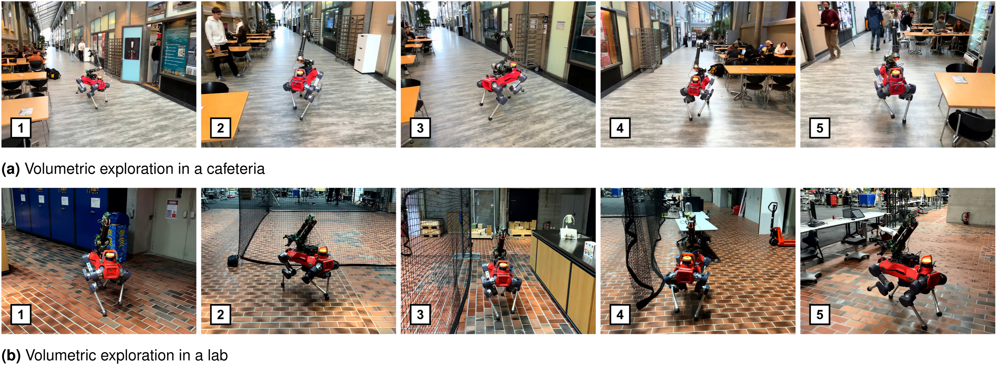
In the first hardware experiment, the robot is tasked with autonomously reconstructing the surface of a lab. We use surface frontiers to estimate gain, allowing the robot to actively navigate toward regions with holes to complete the surface reconstruction. Figure 1 illustrates the reconstructed maps as time evolves. The robot simultaneously explores the environment, expands its graph, and fills in missing holes to produce a more complete surface. While following the planned path, the robot replans at a fixed frequency (omitted from the figure for simplicity). The robot successfully explores this complex and cluttered environment and reconstructs the surface densely, with minimal artifacts such as small holes. We have also conducted surface reconstruction in an outdoor space and an engine museum (Figure 18) and volumetric exploration in a cafeteria and another laboratory environment (Figure 19). These experiments demonstrate the feasibility and effectiveness of running the full planning and perception pipeline onboard the robot across diverse environments. Autonomous surface reconstruction using surface frontiers as the gain. The robot’s trajectory is visualized with a red arrow indicating its direction of movement. The mesh reconstructed from the captured RGB-D images is also shown, with boundary artifacts removed for clarity. Autonomous volumetric exploration using unknown voxels as the gain. Experiments were conducted in both a cafeteria and a lab environment. 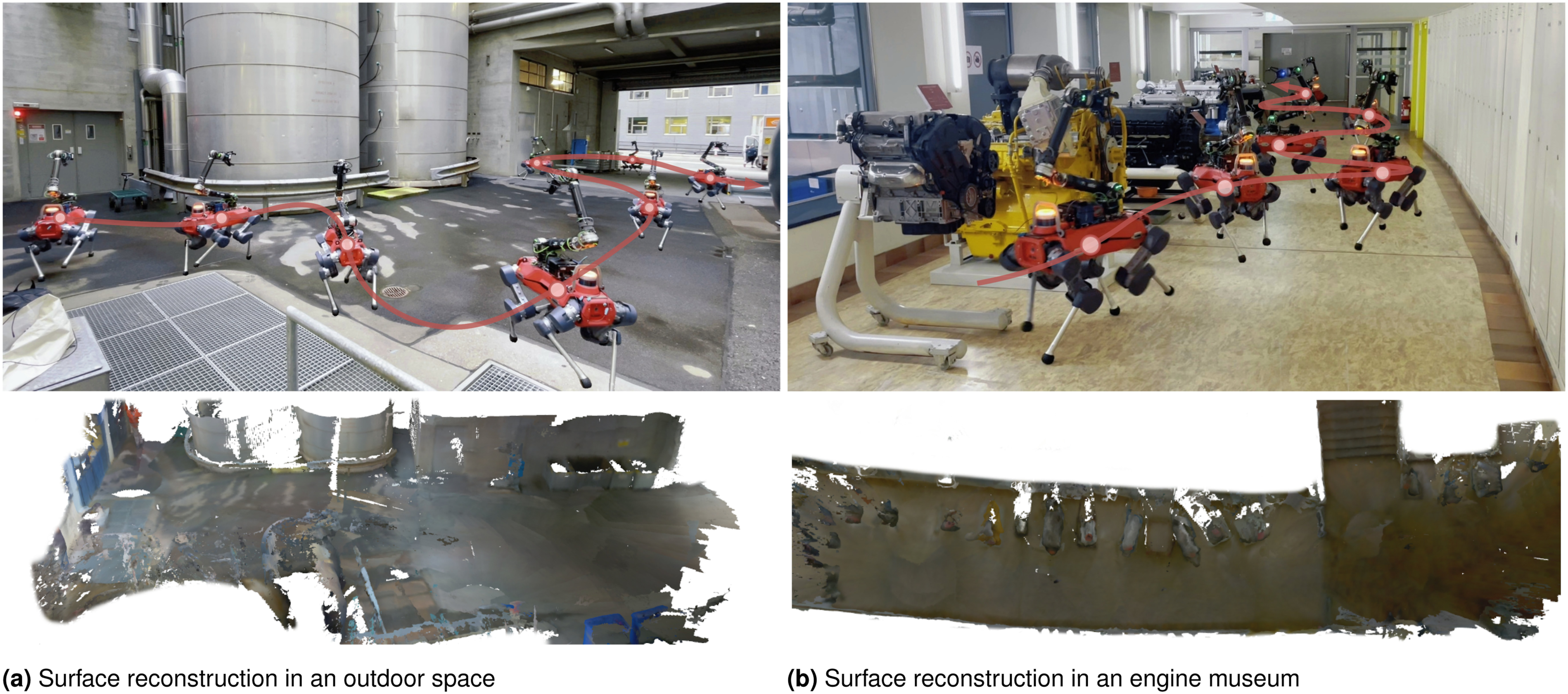
9. Limitations and future directions
While our approach demonstrates strong performance across extensive simulation and hardware experiments, several limitations remain. Our method is validated through empirical evaluation, and we do not provide a formal proof of optimality. Our quantitative evaluation also focuses primarily on indoor environments, as supported by the HSSD dataset, even though we show qualitative hardware results across a broader range of settings (see Figures 1, 18, and 19). Our current framework addresses only semantic-agnostic active perception, and extending it to more challenging semantic tasks is a natural direction for future work. Examples include object-goal navigation, where a robot must find objects in an unknown environment based on natural language instructions (Chang et al., 2024; Gervet et al., 2023; Qu et al., 2024; Shah et al., 2023), and semantic mapping (Fu et al., 2026; Gu et al., 2024; Jatavallabhula et al., 2023; Takmaz et al., 2023; Zhang et al., 2025). In these settings, designing a semantic-aware gain function becomes nontrivial, and it would be compelling to evaluate how our planner performs under such task-driven, semantics-heavy objectives. The present implementation also relies exclusively on ESDF-based mapping. We aim to generalize the planning framework to additional mapping paradigms, particularly 3D Gaussian Splatting (Chen et al., 2025; Goli et al., 2024; Jiang et al., 2023; Kerbl et al., 2023), and to incorporate learned information-gain predictors (Sun et al., 2025). Moreover, while we account for gain correlations in point-collection tasks, we do not model them in volumetric exploration and surface reconstruction. This is because accurately computing inter-node correlations for voxel-counting-based gains is computationally prohibitive—requiring per-voxel tracking to avoid double-counting—and would compromise real-time planning performance. Developing an efficient method to explicitly model correlations between nodes could relax the common additive node-wise gain assumption, thereby improving gain estimation and overall planning performance (Yu et al., 2016).
10. Conclusion
We present NBS, a beam-per-node strategy designed to address the challenges of active perception in mobile robotics. Through extensive empirical evaluation, we show that NBS consistently outperforms classical TSP and SPT baselines as well as naive beam search in graph-based environments. We further demonstrate that the expected gain selection criterion—by incorporating frontier information—achieves a better balance between exploration and exploitation, leading to higher task performance. To bridge abstract graph representations with active perception, we introduce the RRAG, which preserves orientation density and ensures graph connectivity in cluttered environments. In extensive simulations, NBS surpasses state-of-the-art planners across three representative tasks by a significant margin. We validate the practicality of our approach through hardware experiments in different scenarios using onboard computation. All proposed algorithms are available in the open-source
Footnotes
Acknowledgments
The authors would like to thank Jie Tan for the initial discussions, Changan Chen for helpful input, and Boyang Sun and Jiaxu Xing for proofreading the manuscript.
Funding
The authors disclosed receipt of the following financial support for the research, authorship, and/or publication of this article: This research was supported by the Swiss National Science Foundation through the National Centre of Competence in Digital Fabrication (NCCR dfab), by Huawei Tech R&D (UK) through a research funding agreement, and by an ETH RobotX research grant funded through the ETH Zurich Foundation.
Declaration of conflicting interests
The authors declared no potential conflicts of interest with respect to the research, authorship, and/or publication of this article.