Optimisation of the ladle furnace differential flow bottom blowing model using response surface methodology

Abstract

This study investigates the mixing time variations within a 130-ton ladle furnace (LF) using hydraulic experiments to compare the dual-plug equal flow bottom blowing model (Model-EF) and the dual-plug differential flow bottom blowing model (Model-DF). Single-factor analysis was conducted to obtain the optimal porous plug arrangement. Response surface methodology (RSM) was employed to construct a mixing time prediction model based on three factors: high gas flow, low gas flow, and liquid depth, analysing the interaction effects of these factors on mixing time. The results show that the Model-DF with a flow ratio of 2:1 outperformed Model-EF across various porous plug arrangements. The best mixing effect was achieved when the radial position of the porous plugs was 0.57R and the separation angle was 120°, representing an optimisation improvement of 21.05% over the current production Model-EF. The constructed mixing time prediction model exhibited excellent fit, with an R² value as high as 0.9597. Single-factor analysis revealed that the interaction between high gas flow and low gas flow significantly influenced mixing time. Based on this model, three different liquid depths were optimised, yielding corresponding optimal process parameters, which were validated through hydraulic experiments. Experimental results showed that under different operating conditions, the errors between experimental mixing times and predicted values were 2.17%, 1.54%, and 3.77%, respectively. These findings confirmed the effectiveness and reliability of the predictive model, providing new insights and technical support for optimising the LF refining process.

Keywords

Ladle furnace argon bottom blowing Argon stirring gas flow rate hydraulic experiment mixing time response surface methodology differential flow

Introduction

Producing high-quality steel has become one of the core tasks in modern steelmaking processes. Secondary refining technology plays a crucial role in bridging different stages of steel production, significantly enhancing product quality and ensuring production stability.^1,2 Ladle argon blowing is an important method in secondary refining, where argon gas is blown into the bottom of the ladle to improve the flow field distribution within the melt, promote the flotation of inclusions, and homogenise the composition and temperature of the melt, thereby enhancing the cleanliness of the steel.^3–5 In current production processes, improper control of bottom blowing techniques leads to prolonged mixing times of the molten steel. Optimising the arrangement of porous plugs and bottom blowing modes can effectively alleviate these issues, significantly improving refining efficiency and steel quality.^6–11 Due to the high-temperature and opaque nature of the refining process, directly observing flow phenomena inside the reactor is extremely challenging. Therefore, physical models of the reactor are primarily used to investigate internal transport phenomena.¹² In current laboratory studies, hydraulic experiments are commonly employed to explore mixing times within ladles.¹³ Several studies have revealed the impact of multiple factors on mixing time. These experiments demonstrated that mixing time is influenced by various factors and is correlated with bottom blowing flow rates and the arrangement of porous plugs.^14–16

Currently, two porous plugs are typically arranged in large-capacity ladles. For large-capacity ladles, the design of dual porous plugs can effectively meet their demand for more efficient stirring, thereby achieving more uniform molten steel mixing and higher refining efficiency. The traditional equal-flow bottom-blowing mode has the drawback of gas columns colliding and interfering with each other inside the ladle, leading to partial energy dissipation and reduced stirring efficiency.¹⁷ The interference between gas columns makes it difficult to form effective large-scale circulation flows, which is not conducive to the uniform mixing of molten steel. To address the above issues, a dual-hole differential-flow bottom-blowing mode has been proposed. In this mode, the gas flow rates through the bottom-blowing holes are different, generating two streams of gas with one stronger and one weaker kinetic energy above the blowing holes. This creates a large circulation flow in a specific direction. The stronger stream primarily stirs the molten steel, while the weaker stream helps float the inclusions.¹⁸

Numerous scholars have conducted extensive physical experiments to investigate the impact of bottom blowing processes on mixing time, analysing the effects of gas flow rate, liquid depth, radial position of porous plugs, and separation angle on mixing time.^19–21 Tang et al.²² proposed a dual-plug bottom blowing mode with different gas flow rates. Through hydraulic experiments, they compared the stirring effects of two argon blowing methods: varying argon flow rates and constant argon flow rates. They derived empirical relationships between mixing time and other factors, enabling the prediction of mixing time. Wang et al.²³ used Model-DF with different flow ratios to find the optimal bottom blowing ratio that minimised mixing time and slag eye area. They validated the optimisation effects of Model-DF on mixing time under various angles and eccentricities. Jardón-Pérez et al.²⁴ used physical modelling to study the effects of gas velocity and blowing methods on mixing time within ladles. They found that a 3:1 flow ratio in Model-DF resulted in shorter mixing times compared to Model-EF, and was more effective than increasing gas velocity alone. Liu et al.²⁵ considered the effects of gas flow rate, slag layer thickness, single-plug position, and dual-plug angle on mixing time within ladles. They found that under dual-plug conditions, for the same porous plug angle, mixing time decreased with increasing gas velocity. Under the same gas flow rate, mixing time decreased as the porous plug angle increased.

Previous studies have shown that appropriately increasing the bottom blowing flow rate can enhance stirring effects and shorten mixing time within the melt pool. However, increased stirring intensity can also exacerbate slag entrainment. Therefore, multiple factors must be considered when optimising LF bottom blowing processes. Response surface methodology (RSM), as a multi-objective optimisation algorithm, has demonstrated its broad application value in fields such as biomedicine, energy and power, thermal systems, etc.^26–28 In recent years, this method has also been introduced into the metallurgical field to address complex process optimisation problems. Xin Zicheng et al.²⁹ used response surface analysis to establish predictive models for mixing time and slag eye area, investigating the combined effects of gas flow rate, liquid level height and slag layer thickness on mixing time and slag eye area. Through experimental validation, they obtained the optimal combination of process parameters.

However, current research on Model-DF primarily focuses on the effects of single factors (such as gas flow rate, porous plug arrangement and melt depth) on mixing time, lacking studies on the interactions among multiple factors and their impact on mixing time. Moreover, most current studies explore optimal bottom blowing process parameters through extensive experiments and data comparisons but rarely delve deeper into establishing predictive models for the outcomes under multi-factor interactions based on experimental data. Therefore, this study aims to investigate the impact of the interactions among high gas flow, low gas flow, and liquid depth on mixing time during Model-DF refining processes. It seeks to establish a mixing time prediction model using RSM and optimise process parameters based on this model. The effectiveness of the predictive model will be validated through experiments, providing a scientific basis and technical support for optimising LF refining processes. The RSM analysis workflow is shown in Figure 1.

Figure 1.

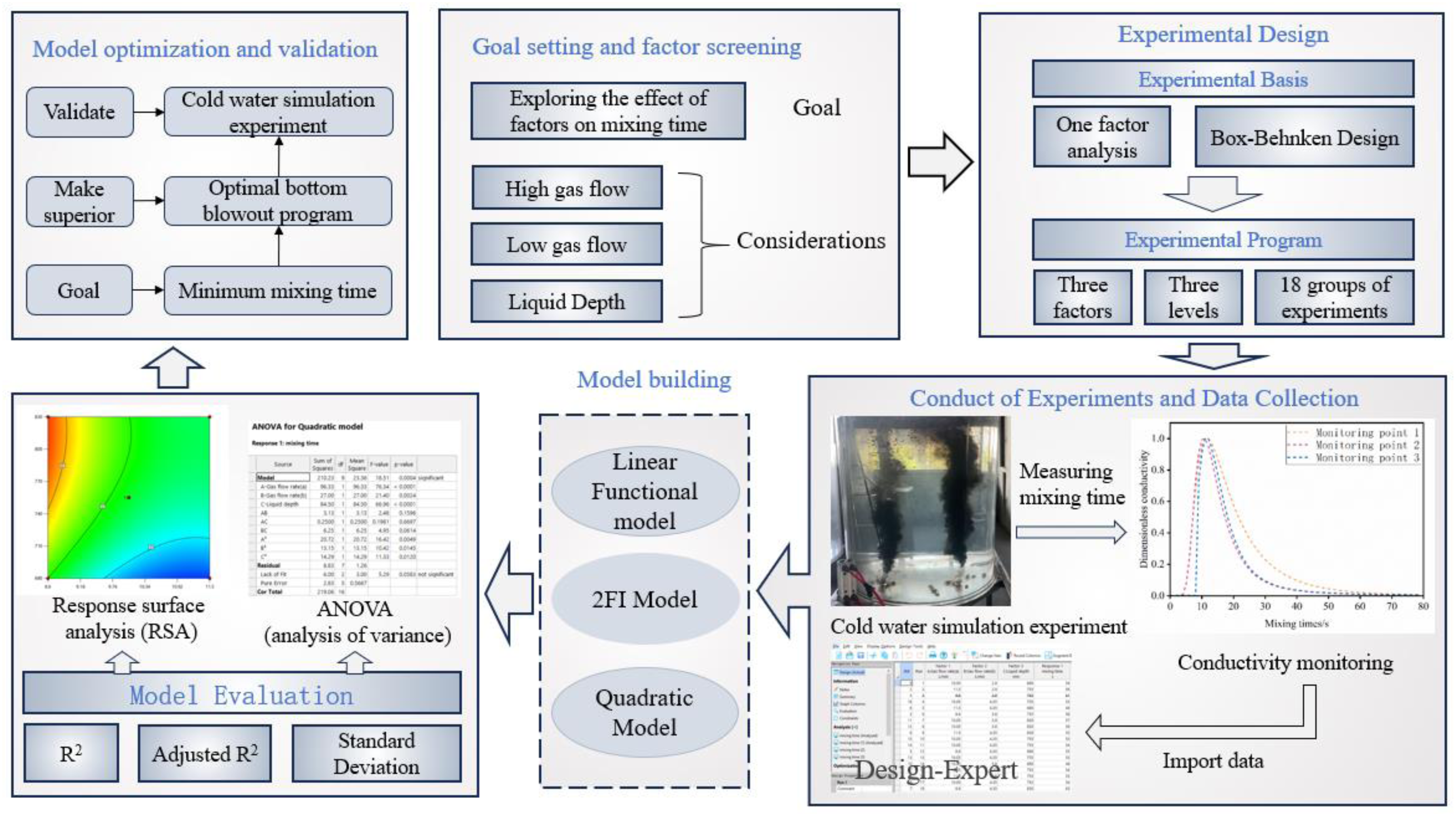
RSM analysis workflow.

Using a 130 t LF refining furnace from a steel plant as a prototype, hydraulic experiments were conducted to investigate the mixing conditions within the ladle under different bottom blowing modes. First, the effects of Model-EF and Model-DF on mixing time were studied under various porous plug arrangements to determine the optimal porous plug layout and the best mixing scheme for each model. Subsequently, single-factor analysis was conducted to study the impact of gas flow rate on mixing time. Based on the experimental data, a mixing time prediction model incorporating high gas flow, low gas flow, and liquid depth was established and its performance was evaluated. Finally, the established model was used to determine the optimal parameters, which were then validated through hydraulic experiments.

Experimental principles and methods

Experimental principles

Geometric similarity

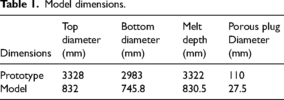
Using a 130 t ladle furnace from a steel plant as a prototype, an acrylic water model was constructed with a geometric similarity ratio of 1:4. To facilitate operation and observation in a laboratory setting and reduce experimental costs, the study employs a geometric similarity ratio of 1:4 and simulates prototype flow behaviour by maintaining a consistent modified Froude number, ensuring the reliability of experimental results. The bottom of the model uses a diffusive permeable element. Relevant dimensional parameters are shown in Table 1.

Table 1.

Model dimensions.

Dimensions	Top diameter (mm)	Bottom diameter (mm)	Melt depth (mm)	Porous plug Diameter (mm)
Prototype	3328	2983	3322	110
Model	832	745.8	830.5	27.5

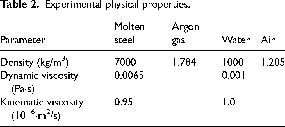
The physical properties of water and air (such as density and viscosity) are similar to those of molten steel and argon, effectively reflecting their flow characteristics. Therefore, water and air are used instead of molten steel and argon for water model experiments. Relevant physical properties are shown in Table 2. The arrangement of porous plugs is shown in Figure 2.

Figure 2.

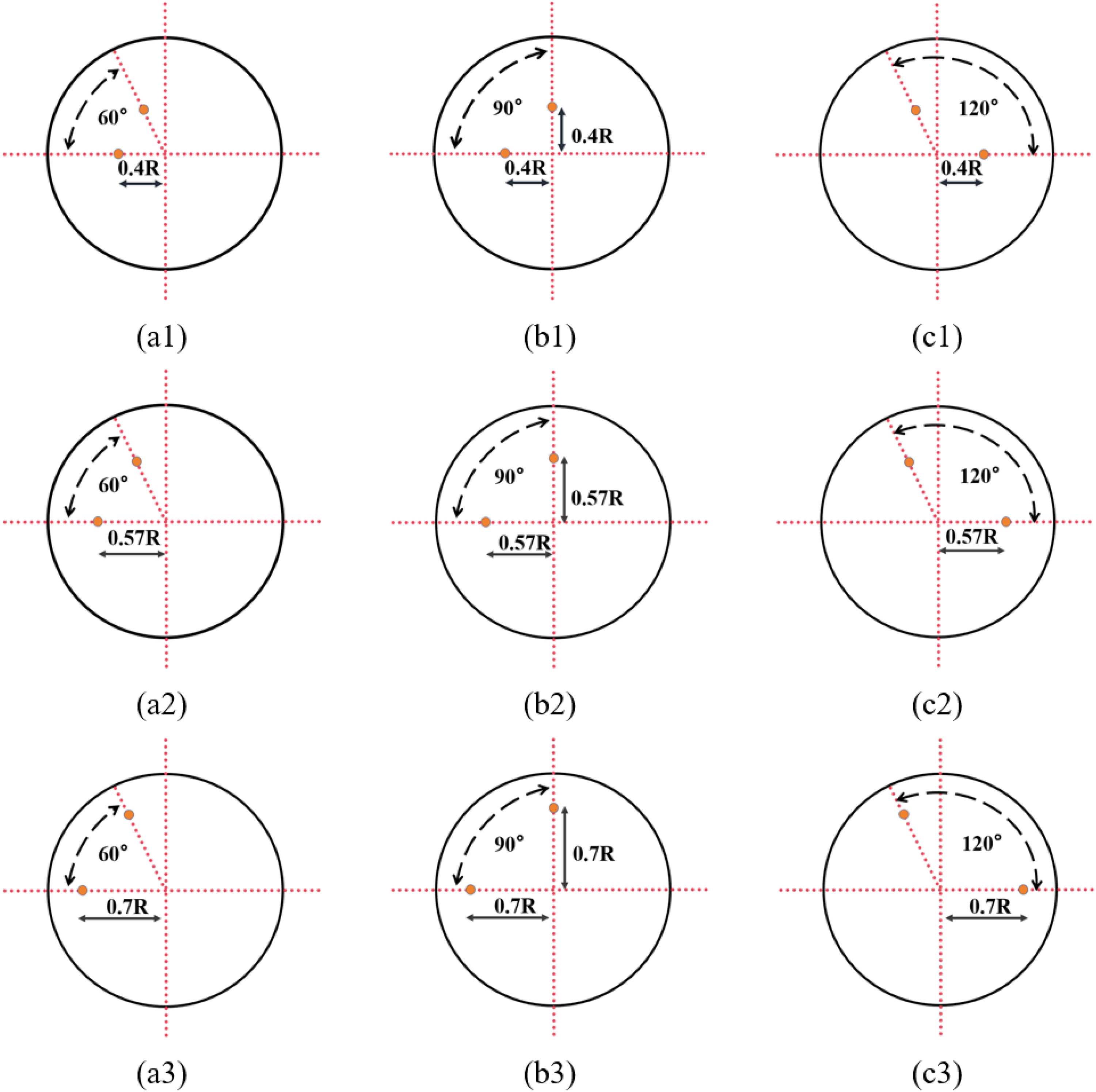
Arrangement of porous plugs: (a) 60°, (b) 90°, (c) 120°.

Table 2.

Experimental physical properties.

Parameter	Molten steel	Argon gas	Water	Air
Density (kg/m³)	7000	1.784	1000	1.205
Dynamic viscosity (Pa·s)	0.0065		0.001
Kinematic viscosity (10⁻⁶·m²/s)	0.95		1.0

The flow of molten steel in the ladle is primarily influenced by gravity, viscous forces, and buoyancy. To maintain dynamic similarity between the prototype and the experimental model, the corrected Froude number should be consistent.^21,30 In a gas–liquid two-phase system, the corrected Froude number can be expressed as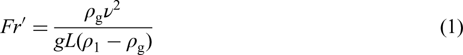

F r^{'} = \frac{ρ_{g} ν^{2}}{g L (ρ_{1} - ρ_{g})}

(1)

where: v is the characteristic velocity, m·s⁻¹, which can be expressed as

4 Q / π d^{2}

; Q is the gas volumetric flow rate, m³·s⁻¹; d is the diameter of the porous plug, m; g is the gravitational acceleration, m·s⁻²; L is the characteristic length, m; ρ_l and ρ_g are the densities of the liquid and gas, kg·m⁻³.

If the corrected Froude number of the experimental model Fr’m is made equal to that of the industrial prototype Fr’pr then the relationship between the bottom-blowing air flow rate Q_m in the experimental model and the bottom-blowing argon gas flow rate Q_p in the industrial prototype can be derived.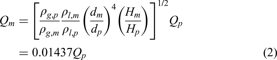

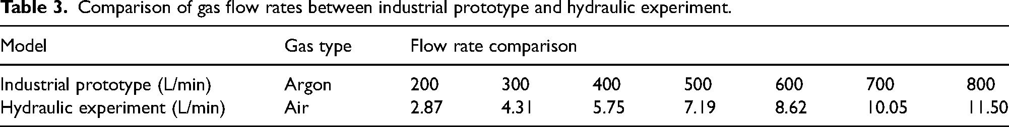
Q_{m} = {[\frac{ρ_{g, p}}{ρ_{g, m}} \frac{ρ_{l, m}}{ρ_{l, p}} {(\frac{d_{m}}{d_{p}})}^{4} (\frac{H_{m}}{H_{p}})]}^{1 / 2} Q_{p} = 0.01437 Q_{p}

(2)

According to Equation (2), the bottom-blowing air flow rate for the hydraulic experiment was calculated. The comparison of bottom-blowing argon gas flow rates in the industrial prototype and bottom-blowing air flow rates in the experimental model is shown in Table 3.

Table 3.

Comparison of gas flow rates between industrial prototype and hydraulic experiment.

Model	Gas type	Flow rate comparison
Industrial prototype (L/min)	Argon	200	300	400	500	600	700	800
Hydraulic experiment (L/min)	Air	2.87	4.31	5.75	7.19	8.62	10.05	11.50

Experimental method

The mixing time was measured using the apparatus shown in Figure 3. The experimental setup consists of three main parts: the gas supply system, the ladle model, and the detection system. The gas supply system comprises an air compressor, a gas tank, valves, and a rotameter, which are connected via flexible air hoses to the porous plugs at the bottom of the ladle model to simulate bottom-blowing argon gas. The detection system includes a computer, a DJ800 multi-functional data acquisition and processing system, data cables, a conductivity metre, and three electrode probes.

Figure 3.

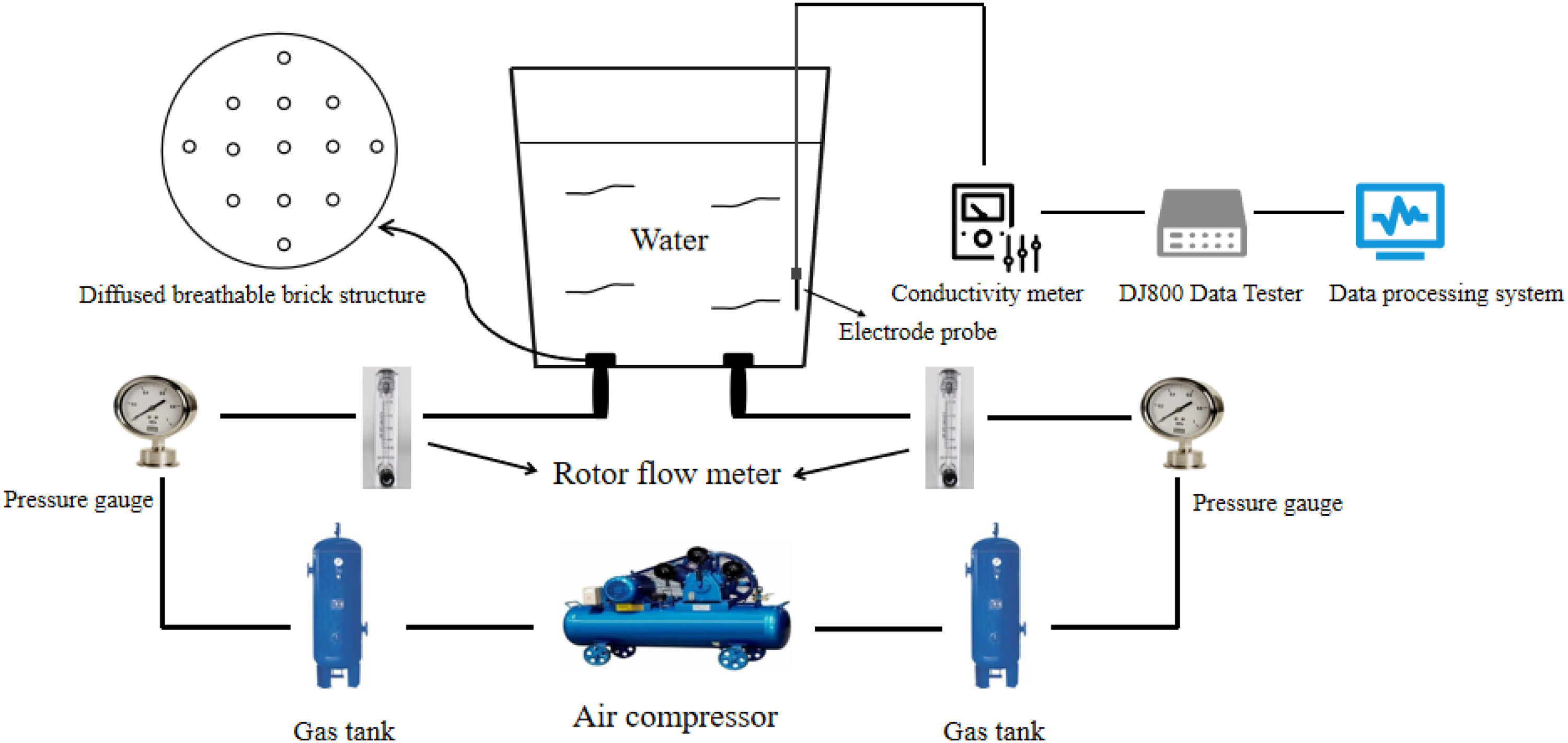
Schematic diagram of hydraulic experiment setup.

Figure 4 shows the placement of the conductivity probes. After opening the gas supply system to introduce air into the ladle model and filling it with water to a specified height, the system is maintained for 3 min until the flow field stabilises. At this point, a fixed amount of saturated KCl solution as a tracer is added at a designated position in the model, and the detection system is activated to collect the conductivity change curves at the electrode positions. After data collection, the conductivity change curves are analysed. When the fluctuation of the conductivity curve does not exceed 5% of the stable value, this time is considered the mixing time at that electrode.^31,32 The longest mixing time among the three electrodes is taken as the mixing time for this experiment. To minimise the impact of experimental errors, each set of experiments is repeated three times, and the average of the three mixing times is taken as the mixing time for that set of experiments.

Figure 4.

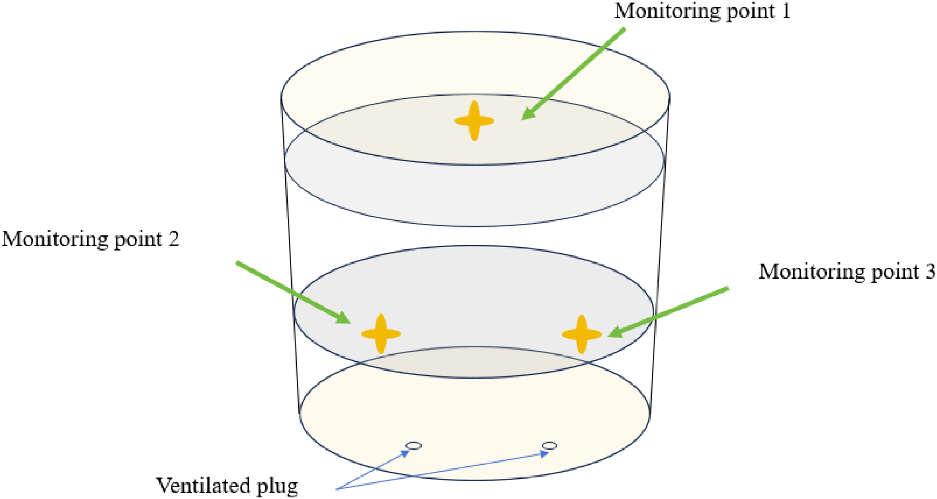
Placement of conductivity probes.

Experimental design

First, the mixing times for Model-EF (Mode 1: 11.5 L + 11.5 L/min, flow rate ratio 1:1) and Model-DF (Mode 2: 11.5 L + 8.62 L/min, flow rate ratio 4:3; Mode 3: 11.5 L + 5.75 L/min, flow rate ratio 2:1) are compared under different porous plug arrangements. Based on the results of this comparison, the optimal porous plug arrangement is determined. Using the optimal porous plug arrangement, the effects of different factors on the mixing time are investigated. RSM is used to design the experimental scheme, establish a model for predicting mixing time, and evaluate and validate this model.

Comparison experimental design for Model-EF and Model-DF

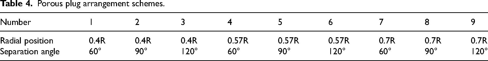
Mixing time is an important metric for evaluating the effectiveness of bottom-blowing agitation, reflecting the uniformity of molten steel under argon stirring. It serves as a critical basis for optimising the arrangement of bottom-blowing holes. The study uses mixing time to determine the optimal direction for configuring the bottom-blowing holes. In the hydraulic experiment model, the radial positions of the porous plugs are 0.4R, 0.57R, and 0.7R, with separation angles of 60°, 90°, and 120°. The porous plug arrangement for the industrial prototype is at a radial position of 0.57R and a separation angle of 90°. The porous plug arrangement schemes are shown in Table 4.

Table 4.

Porous plug arrangement schemes.

Number	1	2	3	4	5	6	7	8	9
Radial position	0.4R	0.4R	0.4R	0.57R	0.57R	0.57R	0.7R	0.7R	0.7R
Separation angle	60°	90°	120°	60°	90°	120°	60°	90°	120°

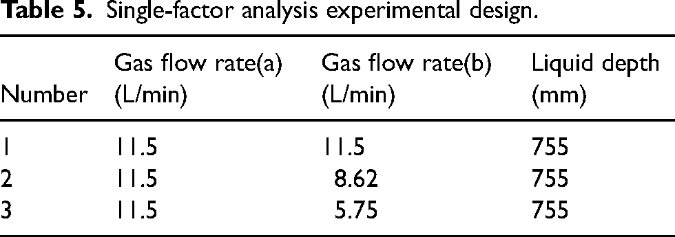
Based on the selected optimal porous plug arrangement, a single-factor analysis is conducted to investigate the effect of gas flow rate on mixing time at a liquid depth of 755 mm. The single-factor analysis experimental design is shown in Table 5.

Table 5.

Single-factor analysis experimental design.

Number	Gas flow rate(a) (L/min)	Gas flow rate(b) (L/min)	Liquid depth (mm)
1	11.5	11.5	755
2	11.5	8.62	755
3	11.5	5.75	755

Experimental design and results based on RSM for bottom-blowing argon

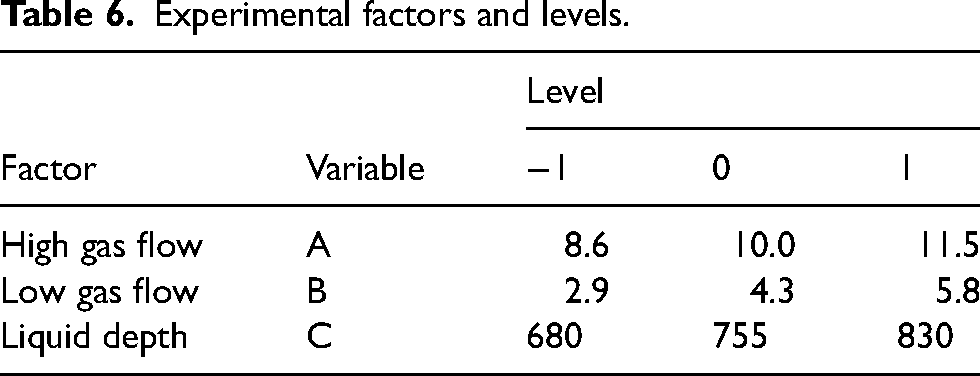
Based on single-factor analysis and the Box–Behnken design (BBD) method, a three-factor, three-level experimental design was developed to analyse the effects of high gas flow, low gas flow, and liquid depth on mixing time, and to determine the mathematical relationship between these factors and mixing time using response surface analysis. During the refining process, the single-hole gas flow rate ranges from 200 to 800 L/min. The minimum and maximum liquid levels of molten steel range from 2720 to 3322 mm. Based on similarity principles, in the hydraulic experiment, the gas flow rate and liquid depth ranges are 2.9–11.5 L/min and 680–830 mm, respectively. The experimental factors and levels are shown in Table 6.

Table 6.

Experimental factors and levels.

Factor	Variable	Level
Factor	Variable	−1	0	1
High gas flow	A	8.6	10.0	11.5
Low gas flow	B	2.9	4.3	5.8
Liquid depth	C	680	755	830

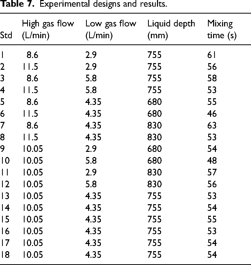
Considering different level combinations of the three factors, 18 experiments were designed. The experimental designs and results are shown in Table 7. These experimental data will be used to construct the subsequent response surface model.

Table 7.

Experimental designs and results.

Std	High gas flow (L/min)	Low gas flow (L/min)	Liquid depth (mm)	Mixing time (s)
1	8.6	2.9	755	61
2	11.5	2.9	755	56
3	8.6	5.8	755	58
4	11.5	5.8	755	53
5	8.6	4.35	680	55
6	11.5	4.35	680	46
7	8.6	4.35	830	63
8	11.5	4.35	830	53
9	10.05	2.9	680	54
10	10.05	5.8	680	48
11	10.05	2.9	830	57
12	10.05	5.8	830	56
13	10.05	4.35	755	53
14	10.05	4.35	755	54
15	10.05	4.35	755	55
16	10.05	4.35	755	53
17	10.05	4.35	755	54
18	10.05	4.35	755	54

Analysis of experimental results

Comparison of hydraulic experiment results for Model-EF and Model-DF

To investigate the impact of Model-DF and Model-EF on ladle mixing, experiments were conducted under different porous plug arrangements for three bottom-blowing modes, recording the corresponding mixing times. The experimental results are shown in Table 8. To more intuitively demonstrate the influence of different bottom-blowing modes on mixing time, a scatter plot of mixing times under different radial positions of porous plugs is drawn as shown in Figure 5.

Figure 5.

Comparison of mixing times for three bottom-blowing modes under different porous plug arrangements.

Table 8.

Comparison of mixing times for three schemes (s).

Bottom-blowing flow rate	Radial position	Separation angle
Bottom-blowing flow rate	Radial position	60°	90°	120°
11.5 L + 11.5 L/min	0.4R	57	57	52
	0.57R	56	57	53
	0.7R	67	64	60
11.5 L + 8.62 L/min	0.4R	58	58	62
	0.57R	53	61	54
	0.7R	58	68	58
11.5 L + 5.75 L/min	0.4R	57	48	49
	0.57R	63	56	45
	0.7R	64	62	53

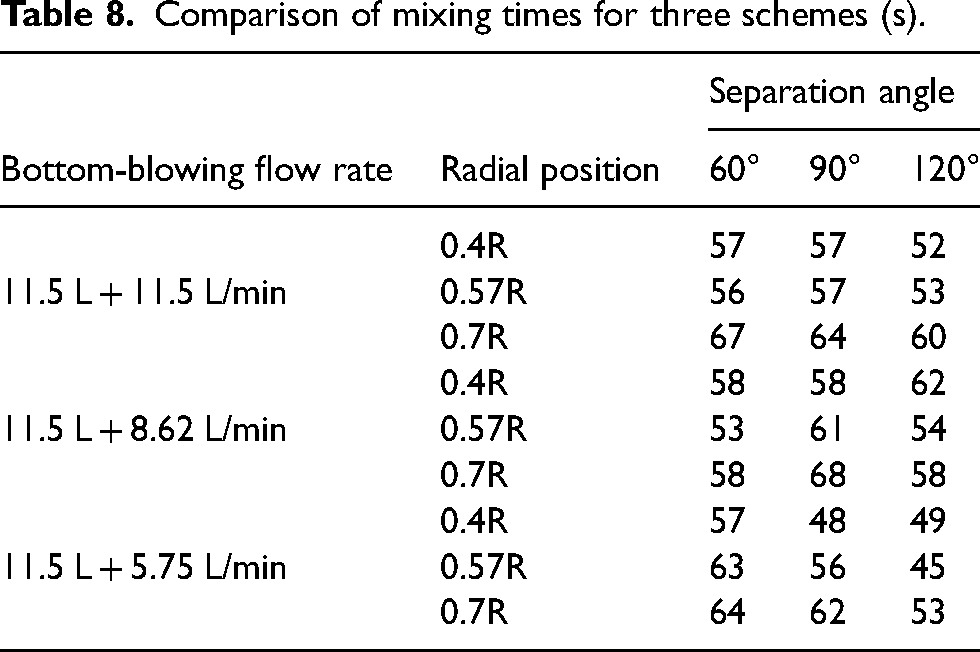
As can be seen from Figure 5, the Model-DF with a flow rate ratio of 2:1 (11.5 L + 5.75 L/min) generally exhibits better mixing effects under different porous plug arrangements compared to Model-EF (11.5 L + 11.5 L/min), except when the radial position is 0.57R and the separation angle is 60°, where the mixing time is longer than that of the dual-plug equal-flow bottom-blowing mode. At radial positions of 0.4R with a separation angle of 90° and at 0.57R with a separation angle of 120°, the mixing time for the Model-DF with a flow rate ratio of 2:1 is shortened by 9 and 8 s, respectively, compared to Model-EF, optimising the bottom-blowing effect by 15.79 and 15.09%, respectively. For the Model-DF with a flow rate ratio of 4:3, compared to the other two bottom-blowing modes, the mixing time is the longest at a radial position of 0.4R; it remains relatively long at radial positions of 0.57R and 0.7R with separation angles of 90° and 120°; however, it is the shortest at radial positions of 0.57R and 0.7R with a separation angle of 60°. The characteristics of Model-EF and the Model-DF with a flow rate ratio of 2:1 are distinct, showing a clear pattern in their impact on mixing time. The Model-DF with a flow rate ratio of 4:3, due to the smaller difference in bottom-blowing flow rates, possesses both the features of equal-flow bottom-blowing and differential-flow bottom-blowing. When the distance between porous plugs is close, its effect is similar to equal-flow bottom-blowing; when the distance is greater, it tends to exhibit characteristics of differential-flow bottom-blowing but shows relatively weaker optimisation in mixing effect.

Additionally, as shown in Figure 5(b), under the conditions of a radial position of 0.57R and a separation angle of 120°, the Model-DF with a flow rate ratio of 2:1 (11.5 L + 5.75 L/min) achieved a mixing time of 45 s, which is the shortest among all schemes, making it the optimal bottom-blowing scheme. Currently, in production, the porous plug arrangement with a radial position of 0.57R and a separation angle of 90° using Model-EF results in a mixing time of 57 s. Compared to the current production scheme, adopting the optimal bottom-blowing scheme can reduce the mixing time by 12 s, achieving an optimisation ratio of 21.05%.

Figure 6 shows the tracer diffusion patterns at different times for Model-EF and the Model-DF with a flow rate ratio of 2:1. From the figure, it can be seen that after the tracer is added at the porous plug location, it rises with the bubble plume and spreads outwards below the horizontal plane, forming an enveloping distribution. This is due to the bubble plume driving the flow of molten steel, creating large-scale circulation which aids in the mixing of the melt pool. By comparing Figure 6(a4) and (b4), it can be observed that after 12 s of adding the tracer, the tracer under Model-DF has a larger diffusion range within the ladle. This indicates that compared to Model-EF, Model-DF can achieve faster melt pool homogenisation, consistent with previous experimental results.

Figure 6.

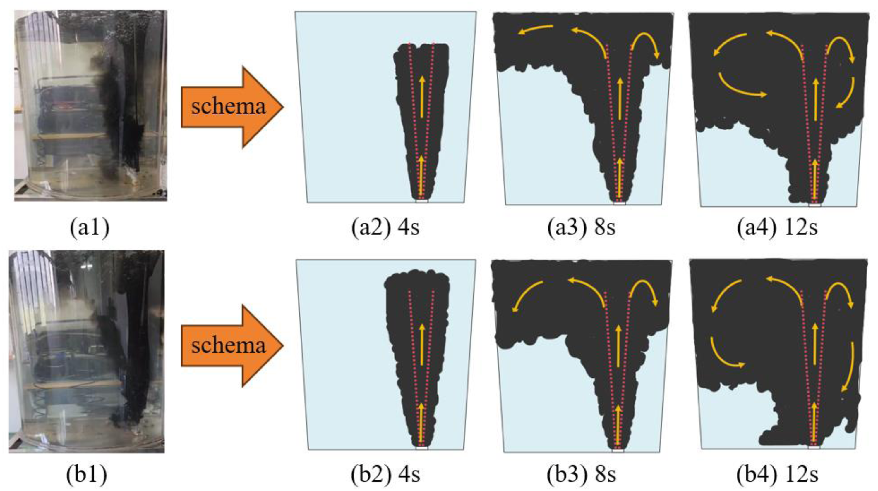
Schematic comparison of mixing conditions at different times for Model-EF (a) and Model-DF with a flow rate ratio of 2:1 (b). (a) Flow rates of 800 and 800 L/min, with a liquid level height of 755 mm; (b) flow rates of 800 and 400 L/min, with a liquid level height of 755 mm.

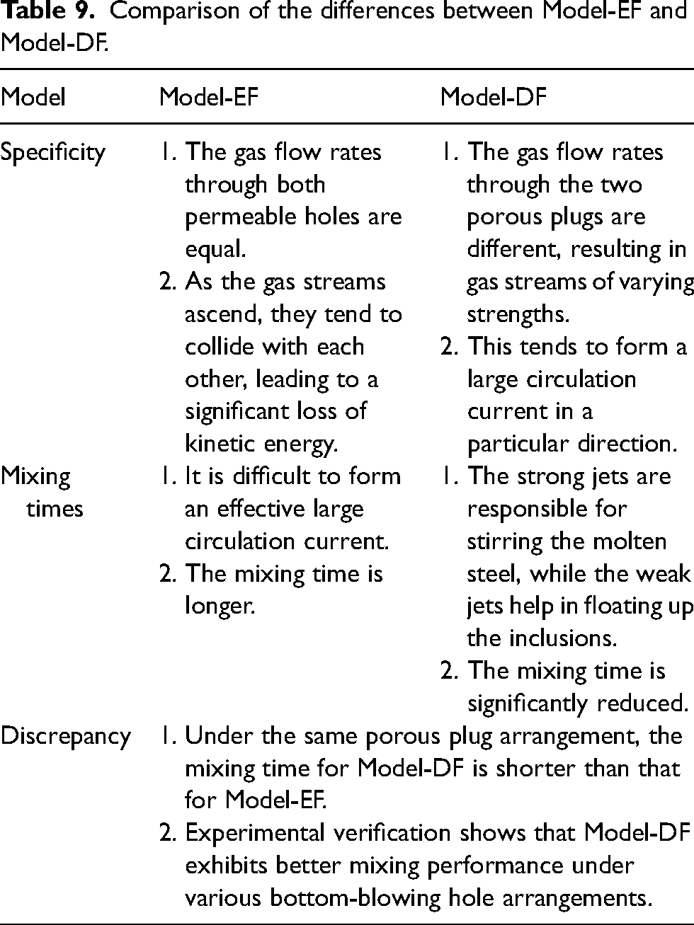
The study compares the Model-EF with the Model-DF and summarises the characteristics and advantages of the two bottom-blowing modes, as shown in Table 9.

Table 9.

Comparison of the differences between Model-EF and Model-DF.

Model	Model-EF	Model-DF
Specificity	1. The gas flow rates through both permeable holes are equal.2. As the gas streams ascend, they tend to collide with each other, leading to a significant loss of kinetic energy.	1. The gas flow rates through the two porous plugs are different, resulting in gas streams of varying strengths.2. This tends to form a large circulation current in a particular direction.
Mixing times	1. It is difficult to form an effective large circulation current.2. The mixing time is longer.	1. The strong jets are responsible for stirring the molten steel, while the weak jets help in floating up the inclusions.2. The mixing time is significantly reduced.
Discrepancy	1. Under the same porous plug arrangement, the mixing time for Model-DF is shorter than that for Model-EF.2. Experimental verification shows that Model-DF exhibits better mixing performance under various bottom-blowing hole arrangements.

Single factor analysis

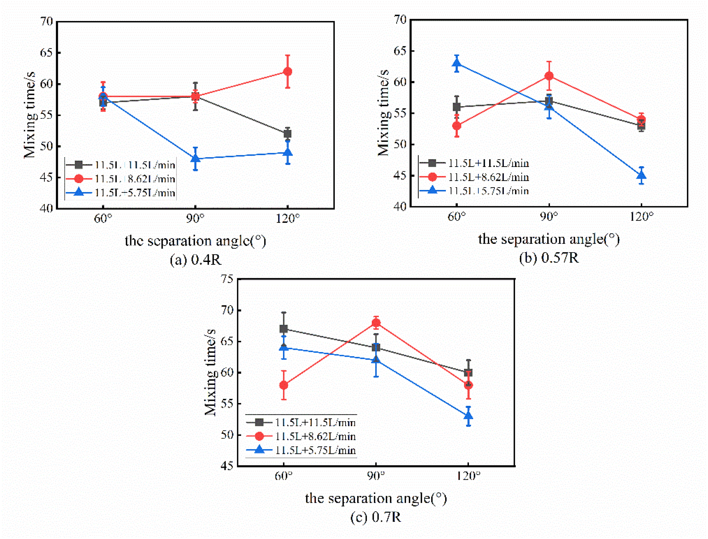
Figure 7 shows the effects of gas flow rate of porous plug b, separation angle of porous plugs, and radial position of porous plugs on mixing time under three different bottom-blowing modes. When the radial position of the porous plug is 0.4R, as shown in Figure 7(a), the mixing time initially increases and then decreases with the reduction in gas flow rate of porous plug b at different separation angles. All three bottom-blowing modes achieve the minimum average mixing time when the separation angle is 120°. In Figure 7(b), when the radial position of the porous plug is 0.57R, all three bottom-blowing modes achieve shorter mixing times at a separation angle of 120°, with the minimum average mixing time still being achieved. From Figure 7(c), it is clearly visible that all three bottom-blowing modes achieve the minimum mixing time at a separation angle of 120°, with the average mixing time significantly leading. Especially, when the radial positions are 0.57R and 0.7R and the gas flow rate of porous plug b is 5.75 L/min, the minimum mixing time of 45 s is achieved under a separation angle of 120°. In summary, the optimal separation angle for porous plugs under all three different bottom-blowing modes is 120°.

Figure 7.

Influence of bottom-blowing modes on mixing time at different radial positions: (a) 0.4R; (b) 0.57R; (c) 0.7R.

Figure 8 shows the influence of gas flow rate of porous plug b, separation angle of porous plugs, and radial position of porous plugs on mixing time from another perspective under three different bottom-blowing modes. As shown in Figure 8(a), when the separation angle is 60° and the radial position of the porous plug is 0.4R, the mixing times for the three bottom-blowing modes are 57 s, 58 s, and 57 s, respectively, with almost identical mixing times. At radial positions of 0.57R and 0.7R, the mixing time initially decreases and then increases as the gas flow rate of porous plug b decreases. The minimum mixing time of 53 s is achieved when the gas flow rate of porous plug b is 8.62 L/min and the radial position is 0.57R.

Figure 8.

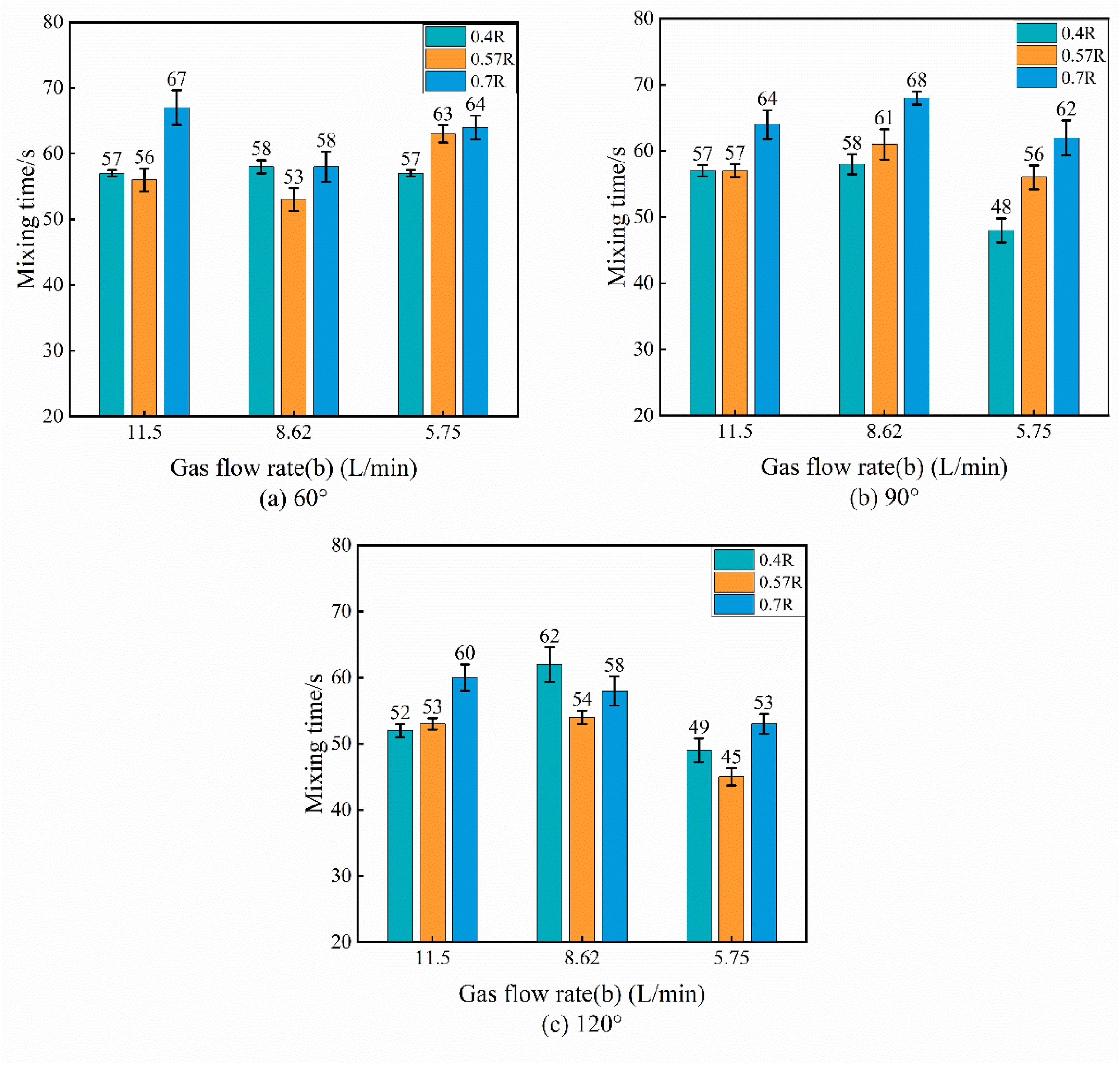
Influence of bottom-blowing modes on mixing time at different porous plug separation angles: (a) 60°; (b) 90°; (c) 120°.

In Figure 8(b), when the separation angle is 90°, the mixing time under all three radial positions initially increases and then decreases as the gas flow rate of porous plug b decreases. The average mixing times for radial positions of 0.4R, 0.57R, and 0.7R are 54.3 s, 58 s, and 64.7 s, respectively. The mixing times for all three bottom-blowing modes perform well at a radial position of 0.4R, with the lowest average mixing time. The average mixing time at a radial position of 0.57R is only 3.7 s longer than at 0.4R, indicating slightly poorer bottom-blowing efficiency at 0.57R compared to 0.4R under a separation angle of 90°. The average mixing time at a radial position of 0.7R is the longest, showing poorer performance.

As can be seen from Figure 8(c), when the separation angle is 120°, at radial positions of 0.4R and 0.57R, the mixing time initially increases and then decreases as the gas flow rate of porous plug b decreases. At a radial position of 0.7R, the mixing time decreases as the gas flow rate of pore b decreases. The average mixing times for the three radial positions are 54.3 s, 50.7 s, and 57 s, respectively, with the shortest average mixing time occurring at a radial position of 0.57R. In the previous section, it was concluded that the optimal separation angle for porous plugs under all three different bottom-blowing modes is 120°. Under this condition, compared to the other two bottom-blowing modes, the bottom-blowing mode with a flow rate ratio of 2:1 (11.5 L + 5.75 L/min) achieves the optimal mixing time at radial positions of 0.4R, 0.57R, and 0.7R. When both plugs are located at 0.4R, the distance between them is relatively close. If the gas flow rates are similar, there is significant interference between the gas columns, leading to collisions between the two rising flow streams and mutual cancellation of kinetic energy. This reduces the stirring effect on the melt pool and extends the mixing time. If the gas flow rates differ significantly, the stronger flow stream dominates the stirring of the melt pool, overcoming the influence of the weaker stream and effectively promoting melt pool movement, thereby reducing the mixing time. When both plugs are located at 0.57R, the distance between them is moderate, resulting in lower interference between the rising flow streams during ascent. Under Model-EF, the flow streams still collide near the free surface, making it difficult to form large-scale circulation, which is not conducive to steel liquid homogenisation. Under Model-DF, the two flow streams have different kinetic energies, forming large-scale circulation along a certain direction within the melt pool, which is more beneficial for steel liquid homogenisation. When both plugs are located at 0.7R, the flow streams are close to the ladle wall, experiencing boundary layer and wall viscous forces during their ascent, leading to partial loss of kinetic energy. This results in poorer stirring effect on the melt pool and longer mixing time.

Analysis of bottom-blown argon experiment results based on RSM

Predictive modelling

Based on the experimental data in Table 7, three different response surface prediction models were constructed: linear function model, two-factor interaction (2FI) model, and quadratic model. The models were evaluated by comparing their R², adjusted R², and standard deviation. The results are shown in Table 10.

Table 10.

Model results.

Model	Mixing time (s)
Model	R ²	Adjusted R²	Standard deviation
Linear function model	0.7733	0.7210	1.95
2FI Model	0.8078	0.6924	2.05
Quadratic model	0.9597	0.9078	1.12

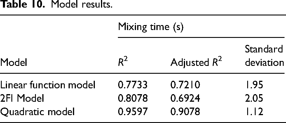
From the above results, it can be seen that the R² and adjusted R² of the quadratic model are 0.9597 and 0.9078, respectively, significantly higher than those of the linear function model and the 2FI model, indicating that the quadratic model has a very high fit. Additionally, the standard deviation is 1.12, significantly lower than the other two models, indicating that the predictions from the quadratic model are more stable and closer to actual observations. In contrast, the linear function model and the 2FI model perform poorly in terms of R² and adjusted R² and have higher standard deviations, resulting in less accurate and less stable predictions. It can be concluded that compared to the linear function model and the 2FI model, the quadratic model better reflects the relationship between bottom-blowing mode, liquid depth, and mixing time in the ladle. Therefore, the quadratic model was chosen to establish the prediction model for mixing time. A regression model for mixing time was established, yielding the regression equation for the independent variables high gas flow (A), low gas flow (B) and liquid depth (C) with the dependent variable mixing time (Y). The regression equation is given in Equation (3).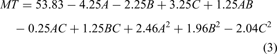

\begin{aligned} M T = 53.83 - 4.25 A - 2.25 B + 3.25 C + 1.25 A B \\ - 0.25 A C + 1.25 B C + 2.46 A^{2} + 1.96 B^{2} - 2.04 C^{2} \end{aligned}

(3)

where: MT is the mixing time, s; A is the high gas flow, L/min; B is the low gas flow rate, L/min; C is the liquid depth, mm.

Model analysis and evaluation

To gain a deeper understanding of the impact of the three factors and their interactions on mixing time, and to evaluate the overall fit of the model, an analysis of variance (ANOVA) was performed on the quadratic model. The results are shown in Table 11. In the ANOVA, F-values and p-values are used to assess whether the contributions of each component of the model to changes in mixing time are significant. When the p-value is less than 0.01, the model is highly significant; when the p-value is between 0.01 and 0.05, the model is significant; when the p-value is greater than 0.05, the model is not significant. The ANOVA results show that the model has a p-value < 0.01, indicating that the model is highly significant overall with good fit, effectively reflecting the relationship between high gas flow, low gas flow, liquid depth, and mixing time during bottom-blowing processes with different flow rates. The influence of each factor on mixing time is as follows: high gas flow (A) >liquid depth (C) >low gas flow (B). Among these, high gas flow (A) and liquid depth (C) reached extremely significant levels, while low gas flow (B) was at a significant level. For the calculated results of interaction terms, the p-values of AB, AC, and BC are all greater than 0.05, indicating that their effects on mixing time are not significant. The p-value for AC is 0.6697, suggesting that the interaction between high gas flow and liquid depth has almost no impact on mixing time. The p-value for AB is 0.1596, indicating that the interaction between low gas flow and liquid depth also has a negligible effect on mixing time. The p-value for BC is 0.0614, slightly exceeding the threshold for model significance, implying that the interaction between low gas flow and liquid depth might have some influence on mixing time under certain conditions. When the bottom-blowing flow rate is small, the stirring capability of the molten steel is weak, and a high liquid level in the melt pool may result in uneven stirring. With a lower liquid level, the limited stirring capacity can better mix the melt pool. Therefore, compared to high gas flow, the interaction between low gas flow and liquid depth has a more significant impact on the mixing time within the ladle. The RSM used in this study is primarily based on a second-order regression model, which has limited ability to detect interactions. In cases where experimental data fluctuates significantly or covers a smaller range, this may result in less pronounced statistical significance for interaction terms. In the results of the quadratic terms, the p-value for A² is less than 0.01, indicating a highly significant effect. The p-values for B² and C² are between 0.01 and 0.05, suggesting that they also have a significant impact on mixing time.

Table 11.

ANOVA analysis table.

Source of variation	Sum of squares	Degrees of freedom	Mean square	F-value	P-value	Significance
Model	210.23	9	23.36	18.51	0.0004	**
A – High gas flow	96.33	1	96.33	76.34	<0.0001	**
B – Low gas flow	27	1	27	21.4	0.0024	**
C – Liquid depth	84.5	1	84.5	66.96	<0.0001	**
AB	3.13	1	3.13	2.48	0.1596	Not significant
AC	0.25	1	0.25	0.1981	0.6697	Not significant
BC	6.25	1	6.25	4.95	0.0614	Not significant
A²	20.72	1	20.72	16.42	0.0049	**
B²	13.15	1	13.15	10.42	0.0145	*
C²	14.29	1	14.29	11.33	0.012	*
Residual	8.83	7	1.26
Lack of fit	6	2	3	5.29	0.0583	Not significant
Pure error	2.83	5	0.5667
Cor total	219.06	16

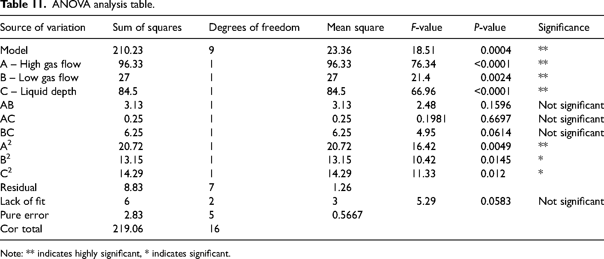
Note: ** indicates highly significant, * indicates significant.

Figure 9(a) shows the normal probability distribution of residuals for mixing time. The points in the plot roughly follow a straight line, indicating that the residuals are normally distributed. Figure 9(b) illustrates the relationship between the actual and predicted values of mixing time. The scatter points in the plot generally follow a straight line, indicating that the model has small prediction errors and that the predicted data closely match the experimental data, demonstrating good predictive performance of the model.

Figure 9.

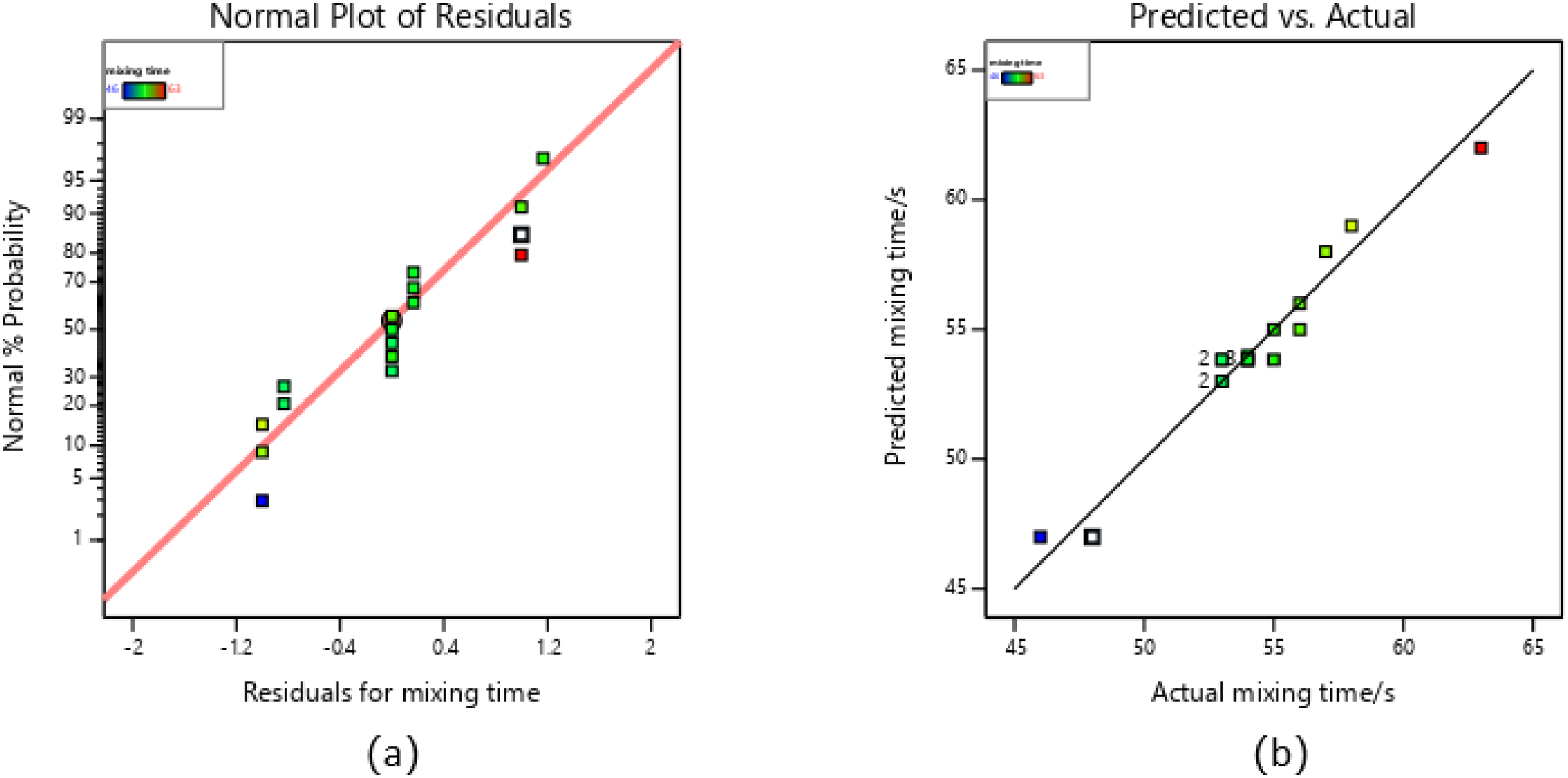
(a) Residual normal probability distribution of mixing time and (b) comparison between actual and predicted values of mixing time.

Response surface analysis

RSM was employed to analyse the mixing time, yielding three-dimensional response surfaces and contour plots that illustrate the interaction effects of the three factors on mixing time, as shown in Figures 10 and 11. In the response surface plots, the steepness of the graph reflects the degree of influence of the factors on mixing time. The steeper the graph, the stronger the interaction between the two factors. In the response surface plots, the steepness of the graph reflects the degree of influence of the factors on mixing time. The steeper the graph, the stronger the interaction between the two factors. In the contour plots, the shape of the graph aids in assessing the strength of the interaction between factors. The closer the shape is to an ellipse, the stronger the interaction between the two factors.

Figure 10.

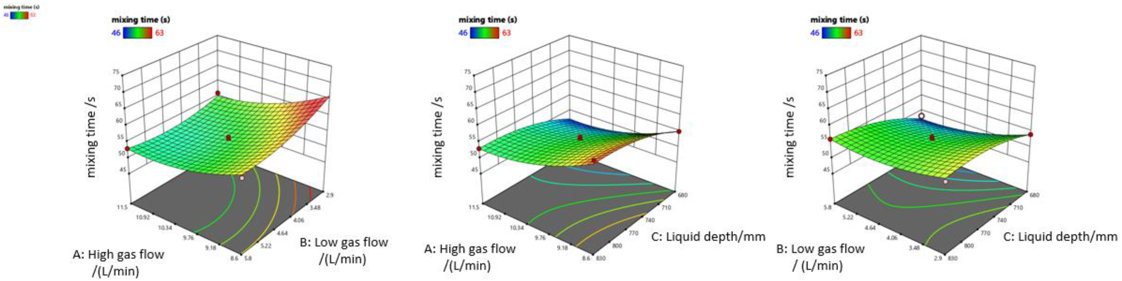
Three-dimensional response surface plots for interactions between different factors: (a) high gas flow and low gas flow, (b) high gas flow and liquid depth, (c) low gas flow and liquid depth.

Figure 11.

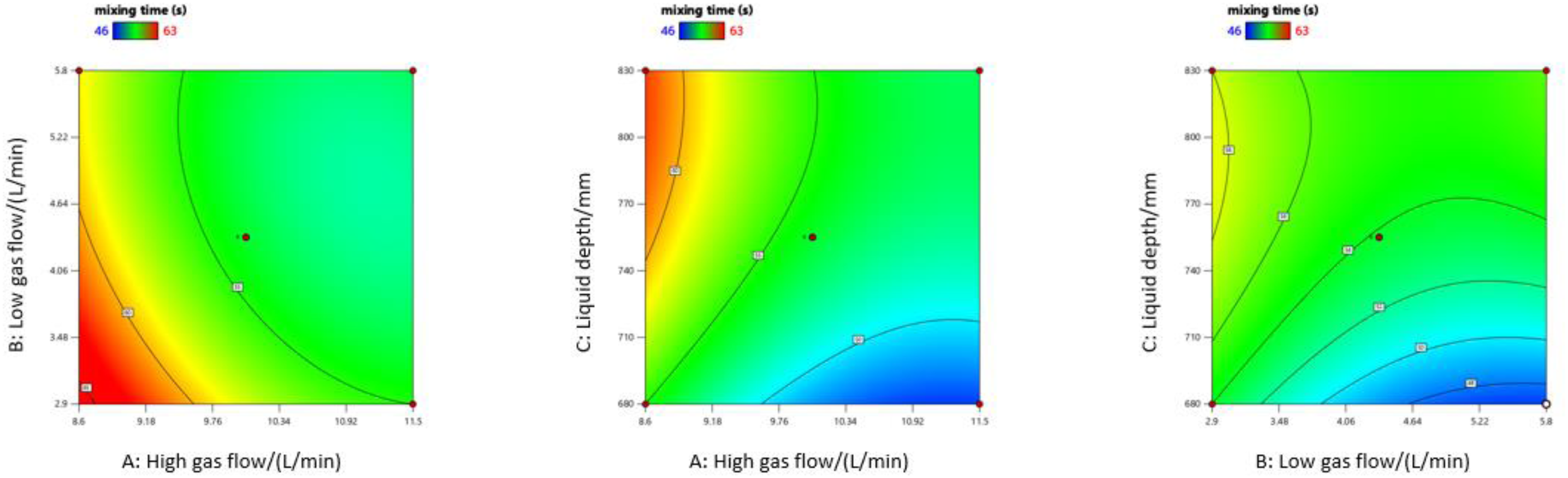
Contour plots of mixing time for interactions between different factors: (a) high gas flow and low gas flow, (b) high gas flow and liquid depth, (c) low gas flow and liquid depth.

Figures 10(a) and 11(a) depict the effect of high gas flow and low gas flow on mixing time when liquid depth is set at 755 mm. As high gas flow increases, mixing time initially decreases and then tends to increase. Increasing low gas flow leads to a decrease in mixing time. Compared to the response surface in the low gas flow direction, the slope of the response surface in the high gas flow direction is greater, indicating a more significant impact on mixing time. Under Model-DF, the mixing time of steel liquid is predominantly influenced by high gas flow. As illustrated in Figure 10(a), with high gas flow increasing from 8.6 to 11.5 L/min, mixing time generally follows a trend of first decreasing and then increasing. This is because the mixing time in the ladle is primarily dominated by high gas flow; as high gas flow increases, the turbulent kinetic energy caused by large circulation due to gas plumes enhances, thereby improving stirring efficiency and reducing mixing time. When high gas flow exceeds 10.34 L/min, mixing time begins to increase. This occurs because excessive bottom-blowing flow beyond a certain range leads to intense turbulence in the steel liquid, disrupting the circulation caused by the rising bubble plume, resulting in longer overall mixing time. Excessive flow causes violent agitation of the steel liquid, potentially leading to slag entrainment and splashing, which can affect the cleanliness of the steel liquid. Increasing low gas flow from 2.9 to 5.8 L/min results in an overall decreasing trend in mixing time, but the reduction is less pronounced compared to high gas flow. Weak bottom-blowing bubble plumes have lower kinetic energy and form recirculation earlier while carrying the steel liquid upward, serving a stirring function on the lower part of the ladle's steel liquid and interacting with large recirculations to promote homogenisation.

Figures 10(b) and 11(b) illustrate the effect of the interaction between high gas flow and liquid depth on mixing time when low gas flow is set at 4.35 L/min. Figures 10(c) and 11(c) show the effect of the interaction between low gas flow and liquid depth on mixing time when high gas flow is fixed at 10.05 L/min. As previously analysed, mixing time initially decreases and then increases with increasing high gas flow, while it decreases with increasing low gas flow. Regarding liquid depth, as liquid depth increases from 680 to 770 mm, mixing time shows an increasing trend. However, from 770 to 830 mm, the rate of increase in mixing time slows down. From Figures 10(b) and 11(b), it can be observed that the slope of the response surface in the high gas flow direction is greater compared to liquid depth, indicating that high gas flow has a more significant impact on mixing time than liquid depth. From Figures 10(c) and 11(c), it can be seen that the slope of the response surface in the low gas flow direction is steeper, indicating that liquid depth has a more significant impact on mixing time compared to low gas flow.

Model-DF optimisation and experimental validation

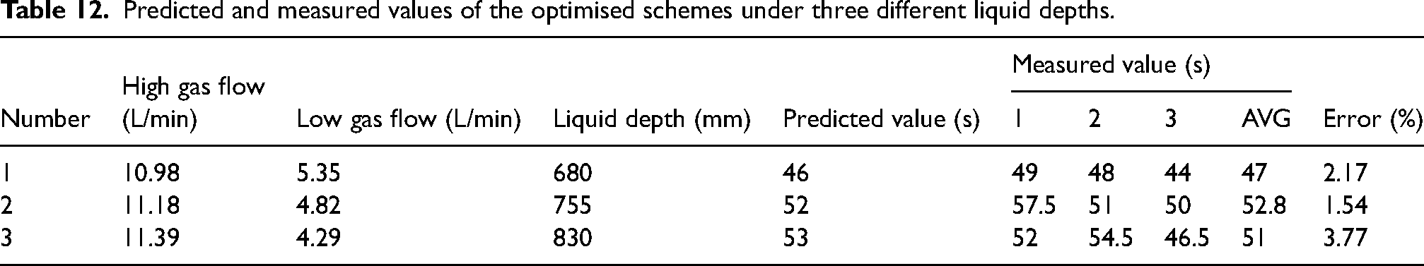
Based on the analysis in section ‘Response surface analysis’, the interaction between high gas flow and low gas flow has a primary influence on mixing time. Using the established mixing time prediction model and aiming to achieve the shortest mixing time, Design-Expert 11 software was utilised to optimise the best conditions for each of the three scenarios with liquid depths of 680, 755 and 830 mm, resulting in three sets of optimal process parameters: (1) for a liquid depth of 680 mm: high gas flow of 10.98 L/min, low gas flow of 5.35 L/min, with a predicted minimum mixing time of 46 s; (2) for a liquid depth of 755 mm: bottom-blowing flow of 11.18 L/min, low gas flow of 4.82 L/min, with a predicted minimum mixing time of 52 s; (3) for a liquid depth of 830 mm: high gas flow of 11.39 L/min, low gas flow of 4.29 L/min, with a predicted minimum mixing time of 53 s. To verify the reliability of the prediction model, hydraulic experiments were conducted using the optimal parameters. The experimental parameters and results are shown in Table 12. From the table, it can be seen that the average measured mixing times for the three sets of parameters were 47 s, 52.8 s, and 51 s, corresponding to predicted values of 46, 52 and 53 s, with measurement errors of 2.17, 1.54 and 3.77%, respectively. The results indicate that under the three optimised conditions, the error between the measured values and predicted values is less than 4%, demonstrating the feasibility of using the response surface-based prediction model to optimise the LF Model-DF.

Table 12.

Predicted and measured values of the optimised schemes under three different liquid depths.

Number	High gas flow (L/min)	Low gas flow (L/min)	Liquid depth (mm)	Predicted value (s)	Measured value (s)				Error (%)
Number	High gas flow (L/min)	Low gas flow (L/min)	Liquid depth (mm)	Predicted value (s)	1	2	3	AVG	Error (%)
1	10.98	5.35	680	46	49	48	44	47	2.17
2	11.18	4.82	755	52	57.5	51	50	52.8	1.54
3	11.39	4.29	830	53	52	54.5	46.5	51	3.77

Research has demonstrated that the mixing time prediction model developed based on RSM effectively reflects the influence of high gas flow, low gas flow, and liquid depth on mixing time. Under experimental conditions, the model exhibits a high degree of fit (R² = 0.9597), accurately predicting mixing time and providing targeted guidance for optimising bottom-blowing processes. This significantly reduces mixing time and improves production efficiency. Using similarity theory, this model can be applied to ladles of different sizes and operating conditions, provided they have the same geometric shape.

However, it must be acknowledged that the model still has certain errors and limitations. The range and quantity of experimental data directly affect the accuracy of the model; insufficient data may lead to increased prediction errors. Additionally, the precision of experimental equipment and measurement errors also impact the model's results. Although hydraulic experiments can effectively simulate the flow field characteristics within a ladle, the high-temperature conditions and complex inclusion distribution in actual industrial production cannot be fully replicated, potentially affecting the predictive accuracy of the model.

Conclusions

Based on a 130 t LF prototype from a steel mill, water model experiments were conducted to investigate the effects of bottom-blowing modes and radial positions of multi-hole plugs on mixing time. Additionally, a mixing time prediction model based on RSM was established. The main conclusions are as follows:

Among different bottom-blowing modes, the shortest mixing time is achieved when the separation angle of the multi-hole plug is 120°. Under this condition, the bottom-blowing mode with a flow ratio of 2:1 achieves optimal mixing times at radial positions of 0.4R, 0.57R, and 0.7R.

The Model-DF with a flow ratio of 2:1 (11.5 L/min + 5.75 L/min) generally exhibits better mixing performance than Model-EF (11.5 L/min + 11.5 L/min) under various multi-hole plug arrangements. Specifically, the minimum mixing time of 45 s is achieved when the radial position of the multi-hole plug is 0.57R and the separation angle is 120°, representing an optimisation ratio of 21.05% compared to the currently used Model-EF in production.

The mixing time prediction model has an R² of 0.9597, an adjusted R² of 0.9078, and a standard deviation of 1.12, indicating good performance. Response surface analysis revealed that the interaction between high gas flow and low gas flow has a primary influence on mixing time, with the impact ranking of the three factors being: high gas flow > low gas flow > liquid depth.

Based on the established prediction model, the optimal process parameters for different liquid depths were optimised. Hydraulic experiments verified the reliability of the optimised schemes, with errors between measured and predicted mixing times all less than 4%, demonstrating the effectiveness and reliability of the prediction model. This provides new insights and technical support for optimising the LF refining process.

Footnotes

Declaration of conflicting interests

The authors declared no potential conflicts of interest with respect to the research, authorship, and/or publication of this article.

Funding

The authors disclosed receipt of the following financial support for the research, authorship, and/or publication of this article: This work was supported by the Tangshan Science and Technology Innovation Program, Natural Science Foundation of Hebei Province, Hebei Province Innovation Ability Improvement Plan (grant numbers 23150219A, A2024108004, E2023209107, 23561001D).

Ethical considerations

This article does not contain any studies with human or animal participants.

ORCID iD

Haobo Qin

References

Emi

. Optimizing steelmaking system for quality steel mass production for sustainable future of steel industry. Steel Res Int 2014; 85: 1274–1282.

Kikuchi

. Development and prospects of refining techniques in steelmaking process. ISIJ Int 2020; 60: 2731–2744.

Castillejos

Brimacombe

. Measurement of physical characteristics of bubbles in gas-liquid plumes: part I. An improved electroresistivity probe technique. Metall Trans B 1987; 18: 649–658.

Chattopadhyay

SenGupta

Ajmani

, et al. Optimisation of dual purging location for better mixing in ladle: a water model study. Ironmak Steelmak 2009; 36: 537–542.

Morales

Calderon-Hurtado

Chattopadhyay

. Demystifying underlying fluid mechanics of gas stirred ladle systems with top slag layer using physical modeling and mathematical modeling. ISIJ Int 2019; 59: 1224–1233.

Conejo

Kitamura

Maruoka

, et al. Effects of top layer, nozzle arrangement, and gas flow rate on mixing time in agitated ladles by bottom gas injection. Metall Mater Trans B 2013; 44: 914–923.

Ramasetti

Visuri

Sulasalmi

, et al. Numerical modeling of open-eye formation and mixing time in argon stirred industrial ladle. Metals (Basel) 2019; 9: 829.

Hua

Bao

Wang

. Multiphysics numerical simulation model and hydraulic model experiments in the argon-stirred ladle. Processes 2022; 10: 1563.

Wang

Zhao

, et al. CFD study on improvement of non-uniform stirring in a large bottom-blown copper smelting furnace. Min Metall Explor 2024; 41: 1421–1435.

10.

Xing

Xiao

Bao

, et al. Process optimization of bottom-blown argon for 130t ladle furnace. Ironmak Steelmak 2023; 50: 894–899.

11.

Safavi Nick

Teng

Yang

, et al. Mathematical modelling of novel combined stirring method during the final stage of ladle refining. Ironmak Steelmak 2023; 50: 721–733.

12.

Sahai

Emi

. Criteria for water modeling of melt flow and inclusion removal in continuous casting tundishes. ISIJ Int 1996; 36: 1166–1173.

13.

Liu

Ersson

Liu

, et al. A review of physical and numerical approaches for the study of gas stirring in ladle metallurgy. Metall Mater Trans B 2019; 50: 555–577.

14.

Conejo

Zhao

Zhang

. On the limits of the geometric scale ratio using water modeling in ladles. Metall Mater Trans B 2021; 52: 2263–2274.

15.

Maldonado-Parra

Ramírez-Argáez

Conejo

, et al. Effect of both radial position and number of porous plugs on chemical and thermal mixing in an industrial ladle involving two phase flow. ISIJ Int 2011; 51: 1110–1118.

16.

González-Bernal

Solorio-Diaz

Ramos-Banderas

, et al. Effect of the fluid-dynamic structure on the mixing time of a ladle furnace. Steel Res Int 2018; 89: 1700281.

17.

Tang

Liu

Zhang

, et al. A novel dual plugs gas blowing mode for efficient ladle metallurgy. Ironmak Steelmak 2019; 46: 405–415.

18.

Yasipourtehrani

Strezov

Bliznyukov

, et al. Investigation of thermal properties of blast furnace slag to improve process energy efficiency. J Cleaner Prod 2017; 149: 137–145.

19.

Chen

Tao

, et al. Effect of salt solution tracer dosage on the transport and mixing of tracer in a water model of asymmetrical gas-stirred ladle with a moderate gas flow rate. Symmetry (Basel) 2024; 16: 619.

20.

Ouyang

Wang

, et al. Physical simulation study on flow field characteristics of molten steel in 70t ladle bottom argon blowing process. Metals (Basel) 2023; 13: 639.

21.

Sun

Zhang

Lin

, et al. Effect of bottom blowing mode on fluid flow and mixing behavior in converter. Metals (Basel) 2022; 12: 117.

22.

Haiyan

Xiaochen

Guanghui

, et al. Effect of gas blown modes on mixing phenomena in a bottom stirring ladle with dual plugs. ISIJ Int 2016; 56: 2161–2170.

23.

Wang

Liu

, et al. Effect of differential flow blowing argon and nozzle position on mixing time and slag eye in dual nozzle ladle using water model experiment. Metall Mater Trans B 2024; 55: 2209–2223.

24.

Jardón-Pérez

González-Morales

Trápaga

, et al. Effect of differentiated injection ratio, gas flow rate, and slag thickness on mixing time and open eye area in gas-stirred ladle assisted by physical modeling. Metals (Basel) 2019; 9: 555.

25.

Liu

. Modeling of gas-steel-slag three-phase flow in ladle metallurgy: part I. Physical modeling. ISIJ Int 2017; 57: 1971–1979.

26.

Hussain

Panchal

Allamraju

, et al. Optimization of wear behavior of heat-treated ti-6Al-7Nb biomedical alloy by response surface methodology. Environ Res 2023; 231: 116193.

27.

Tan

, et al. Performance optimization of a diesel engine fueled with hydrogen/biodiesel with water addition based on the response surface methodology. Energy 2023; 263: 125869.

28.

Matheswaran

Arjunan

Muthusamy

, et al. A case study on thermo-hydraulic performance of jet plate solar air heater using response surface methodology. Case Stud Therm Eng 2022; 34: 101983.

29.

Xin

Sun

Zhang

, et al. Multiobjective collaborative optimization of argon bottom blowing in a ladle furnace using response surface methodology. Mathematics 2022; 10: 2610.

30.

Xiao

Peng

. Mathematical modelling of entrapment phenomena at slag/metal interface in gas-stirred ladle. Iron Steel(China) 1989; 24: 17–21.

31.

Pan

Björkman

. Numerical analysis on the similarity between steel ladles and hot-water models regarding natural convection phenomena. ISIJ Int 2002; 42: 53–62.

32.

Han

Heo

Kam

, et al. Transient fluid flow phenomena in a gas stirred liquid bath with top oil layer—approach by numerical simulation and water model experiments. ISIJ Int 2001; 41: 1165–1172.