Study on the vision transformer numerical regression based prediction model of the outlet induction heating set temperature for a hot-dip galvanised steel strip

Abstract

The quality of galvanising alloying for a continuous hot-dip galvanised steel strip subjected to the induction heating (IH) treatment after being delivered out of a zinc pot can be effectively improved. The temperature of an IH outlet setting strip represents a key factor affecting the alloying quality. However, traditional prediction models have low accuracy, which requires additional manual intervention and poses difficulty in improving the quality of coating alloying. To address these challenges, this study proposes the vision transformer-based algorithm for numerical data regression, named the vision transformer numerical regression (ViTNR) algorithm. In addition, using the historical datasets of IH outlet strip temperature in the hot-dip galvanising production, this study develops a ViTNR prediction model for IH outlet setting strip temperature. The proposed ViTNR model of IH outlet strip setting temperature is compared with four typical deep learning-based models, including convolution neural networks, and five shallow learning-based models, including the AdaBoost model. The comparison results show that the proposed ViTNR model can achieve higher prediction accuracy and better generalisation ability in the IH outlet strip temperature prediction application scenarios compared to the comparison models.

Keywords

induction heating deep learning outlet strip temperature attention mechanism hot-dip galvanising

Introduction

In the manufacturing industry, steel is an indispensable structural material, and galvanised strip steel is an important steel product with the advantages of high strength, toughness, corrosion resistance, surface quality, processing and forming performance, and convenient transportation and storage.¹

Common methods for galvanising strip steel include continuous or batch hot dip galvanising, electric galvanising, spray galvanising, mechanical electroplating and spraying zinc-rich paint.² Among them, hot dip galvanising represents the main production process of industrial galvanising, which has the advantages of high efficiency and relatively low cost. For automotive plates and other high-value-added hot dip galvanised strip steel products, the coating has high-quality requirements. Namely, after exiting the zinc pot and passing through the air knife, the strip steel enters the induction heating (IH) furnace for IH to conduct the alloying of the strip steel coating (Galvanneal, GA). The alloying IH process has the advantages of rapid metal surface heating, simple temperature control and energy saving.³

The temperature of an IH outlet strip is the most critical parameter in GA product production, and it directly affects key properties, such as zinc layer adhesion; it can also cause quality-related problems, such as incomplete alloying (i.e., white edges). The alloying process of hot dip galvanised GA products is complex and includes many tasks, such as heat transfer and temperature changes, metal diffusion and alloying reaction on the coating surface. The IH outlet strip temperature is set based on many factors, such as process speed, annealing furnace temperature, zinc pot temperature, alloy element content in zinc liquid and alloying furnace temperature. However, the relationship between the IH outlet strip temperature and process parameters is complex and highly nonlinear.^4,5

The traditional method for determining the most convenient IH outlet strip temperature is to calculate the empirical formula, which represents a linear equation of the coating's target thickness and the unit's linear speed. However, the empirical formula cannot accurately reflect the nonlinear relationship between the IH outlet strip temperature and various influencing factors, which results in low calculation accuracy. In addition, the determination of the temperature of an IH outlet setting strip in online production requires manual intervention, which restricts the improvement of GA coating alloying quality.

With the development of modelling theory based on big data, the development of data-driven prediction models based on machine learning has become an effective method for establishing nonlinear relationships in complex industrial processes and improving prediction accuracy. This method has been successfully applied to many metallurgical processes, such as hot rolled strip width (SW) prediction and continuous annealing furnace process settings.^6–8

According to the number of hidden layers, data-driven machine learning-based prediction models can be roughly divided into shallow learning-based models and deep learning-based models. The shallow learning-based models have fewer hidden layers, and they include support vector machine (SVM), k-nearest neighbours (KNN), decision tree and related integrated learning-based algorithms. In addition, backpropagation neural network models with fewer hidden layers can also be classified as shallow learning-based models. Deep learning-based models have many hidden layers, usually more than five. Representative deep learning-based algorithms include convolutional neural networks (CNNs) and deep neural networks (DNNs).^9–11

Considering shallow learning-based prediction models, Ding Luxi et al.¹² selected the strip running speed, which has the greatest influence on the strip coiling temperature, as a prediction index to improve the control accuracy of strip coiling temperature. The dataset was standardised based on the Z-scores, and the optimal hyperparameters were found by grid search. In addition, the gradient boosting decision tree (GBDT), random forest (RF) and SVM export speed prediction models for hot-rolled strip steel were established and compared, and the results showed that the GBDT model had the highest prediction accuracy among the tested models. Therefore, this model could effectively improve the precision of coiling temperature control. Qu et al.¹³ sought to address the inaccuracy of the model between gas flow and temperature in the annealing furnace temperature control system. To this end, they established a gas flow prediction model for the annealing furnace by employing the SVM algorithm. They then optimised the model's hyperparameters by utilising the genetic algorithm. Finally, they employed field production data as test samples to verify the reliability and accuracy of the model.

Studying deep learning-based prediction models, Xie et al.¹⁴ constructed a prediction model for the mechanical properties of a hot-rolled thick plate based on the DNN algorithm. The main aim was to address complex and challenging relationships between process parameters and mechanical properties in steel plate production. The authors also analysed the impact of the DNN structure and hyperparameters on the model's properties. The prediction accuracy of the DNN, SVM, RF and five other types of machine learning models was compared. The comparison results showed that the DNN model achieved the highest prediction accuracy among all models; it could realise online monitoring and control of mechanical properties of the hot rolled thick plate in steel mill application. He et al.¹⁵ proposed a novel prediction model that integrates the advanced techniques of a generalised radial basis function neural network and composite expectation regression. This innovative approach was developed to address the challenges posed by nonlinearity and data heterogeneity in modelling. Extensive experimental evaluations have demonstrated the efficacy of the proposed model, substantiating its high prediction accuracy.

For the CNN models whose input features are numerical, in addition to feeding one-dimensional numerical data directly to the model input, a data-filling method can also be used to convert one-dimensional numerical data into two-dimensional image data that is then input to the model. This data dimension expansion makes a prediction model apply the training data more fully, and this strategy has attracted increasing attention in recent research.

Xu et al.¹⁶ proposed a CNN method for predicting the mechanical properties of the hot-rolled strip steel, considering the chemical composition and process parameters. In addition, a small convolution kernel and a small pooling region were adopted in the CNN structure to reduce the number of model parameters and improve the model's generalisation ability. The prediction accuracy was higher than that of the SVM model. Li et al.¹⁷ addressed the problem of predicting the mechanical properties of hot-rolled strip steel using a simplified Inception module to construct a convolutional network for predicting mechanical properties (CNPMP). They optimised the network structure and compared the proposed model with nine machine learning-based models, such as the SVM and RF. The comparison results showed that the CNPMP model could achieve higher prediction accuracy than the other models.

Transformer is an advanced type of DNN architecture which does not contain a convolutional layer and adopts an attention mechanism and a full connection layer to process sequence data. Transformer and its derivative algorithms have advantages in the fields of natural language processing and image processing over other algorithms [.¹⁸ Vision Transformer is a typical Transformer derivative algorithm, which simplifies the Transformer's structure while improving its performance in image classification and large-scale image processing.¹⁹

To improve product quality, this study proposes a method for predicting the temperature of a hot-dip galvanising IH outlet setting strip, which employs a Vision Transformer deep learning-based algorithm. In addition, a Vision Transformer numerical regression (ViTNR) model is constructed, and Vision Transformer is applied to the field of regression prediction, adjusting the model's hyperparameters. Finally, the prediction performance of nine learning models, including the CNN and DNN models, is analysed and compared on the test dataset.

Method

Big data processing and feature screening

The production process of hot-dip galvanised GA steel sheets includes uncoiling, welding of the front and rear ends of coils, cleaning residual oil and iron from the strip surface, annealing and cooling, hot-dip galvanising in a zinc pot, controlling the weight and thickness of the zinc layer using an air knife and IH in an alloying furnace.

Developing an efficient and accurate temperature prediction model of a hot-dip galvanising IH outlet setting strip is a key process in parameter prediction modelling. The prediction model uses an IH outlet setting strip's temperature, which is the most critical in the alloying IH process, as output, and the factors affecting the temperature of a setting strip are used as input for production control. To this end, this study selects 22,712 high-quality data samples obtained from the historical big data on the hot-dip galvanised process accumulated by steel mills and uses the coating alloying quality index as a modelling dataset. The modelling dataset includes a total of 21 feature parameters, such as specifications and strip temperature. The statistical results of some feature parameters are shown in Table 1.

Table 1.

Statistical results of some characteristic parameters of the modelling dataset of the IH outlet setting strip temperature prediction model.

Feature	Unit	Minimum value	Maximum value	Mean value	Standard deviation
ST	mm	0.68	2.32	1.49	0.35
SW	mm	806.00	1526.00	1052.28	168.07
ZWT	g/m²	70.00	110.00	97.32	9.01
PS	m/min	50.00	123.00	80.19	14.50
JCFT	°C	451.00	520.00	469.56	10.42
THFT	°C	440.00	549.00	531.05	14.84
IHST	°C	492.00	570.00	534.29	9.62

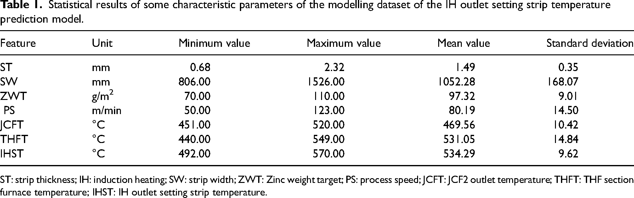
ST: strip thickness; IH: induction heating; SW: strip width; ZWT: Zinc weight target; PS: process speed; JCFT: JCF2 outlet temperature; THFT: THF section furnace temperature; IHST: IH outlet setting strip temperature.

The Z-score method is used to detect outliers in the IH outlet setting strip temperature modelling dataset. The points with an absolute Z-score larger than three are removed from the dataset, yielding a dataset consisting of 18,320 data samples.

In the research of IH outlet setting strip temperature modelling, the accuracy of models, such as the GBDT, RF and AdaBoost, which use decision trees as base learners, is not affected by the scale of input features; therefore, no normalisation is required in the prediction model design. However, the accuracy of other shallow and deep learning-based models is affected by the dimension of input features. To ensure the convergence speed and performance of the fitted models, this study uses the Min-Max Scaling to normalise the dataset.

The temperature of an IH outlet strip is an important factor affecting the alloying process and coating quality. The output of the IH outlet strip temperature prediction model is the IH outlet strip temperature value, and important factors related to the IH outlet temperature denote the model's input data.

According to the metallurgical mechanism, the following four types of features are selected in this study as input features for initial screening:^20–23

Strip steel specification features: Strip thickness (ST) and SW;

Basic chemical element features: Effective aluminium content in zinc solution;

Zinc coating weight features: Zinc coating weight target (Zinc weight target: ZWT) and online zinc layer weight average;

Processing technology parameter features: Process section speed (process speed: PS), annealing JCF2 section temperature (JCFT), THF section furnace temperature (THFT) and zinc bath temperature.

Alloying Furnace #1 Holding Section Position 1 Temperature (AF1T#1);

Alloying Furnace #1 Holding Section Position 2 Temperature (AF1T#2);

Alloying Furnace #2 Holding Section Position 1 Temperature (AF2T#1);

Alloying Furnace #2 Holding Section Position 2 Temperature (AF2T#2)

The factors influencing the alloyed coating properties selected by the metallurgical mechanism could be mutually coupled; thus, there might be redundant characteristics. In view of that, this study uses the Pearson correlation coefficient method for analysis. The correlation coefficient threshold is set to 0.8, and redundant features AF1T#2, AF2T#2 and ZWT are removed. After feature screening, the number of remaining input features becomes 10.

Multi-head attention mechanism

Similar to the human tendency to focus on valuable information while ignoring other information when perceiving the world, in the deep learning field, the means of using limited resources to extract high-value information are denoted as attention mechanisms. The introduction of an attention mechanism into the Transformer algorithm can significantly improve the efficiency and accuracy of information processing. In addition, it has great advantages in many other fields, including natural language processing and image processing.¹⁸

Before the input attention mechanisms, three trainable linear transformations are performed on each embedded vector, transforming it into query information (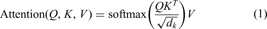 q ), corresponding key information ( k ), and value information ( v ). Assume that the dimensions of query and key information are denoted by d_k, and the dimension of value information is denoted by d_v; then, the query information is dot-multiplied with the corresponding key information, divided by $\sqrt{d_{k}}$ , and processed by a softmax function to obtain the weights of value information. This yields the output data of the attention mechanism. If the query information matrix, key information matrix, and value information matrix are denoted by Q , K and V , respectively, then the attention mechanism matrix's output is expressed by:

\begin{matrix} Attention (Q, K, V) = softmax (\frac{Q K^{T}}{\sqrt{d_{k}}}) V \end{matrix}

(1)

As shown in Figure 1, a multi-head self-attention (MSA) mechanism represents an extension of the attention mechanism. Suppose that query information, key information and value information are projected to d_k, d_k and d_v dimensions, respectively, for h times by different learnable linear projections (Linear). Then, the attention function is calculated in parallel for the projections of the query, key, and value information to obtain the output value of a dimension d_v. This information is then connected and projected again to obtain the output value (M) of the multi-head attention mechanism. The calculation process can be expressed as follows: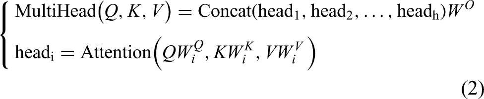

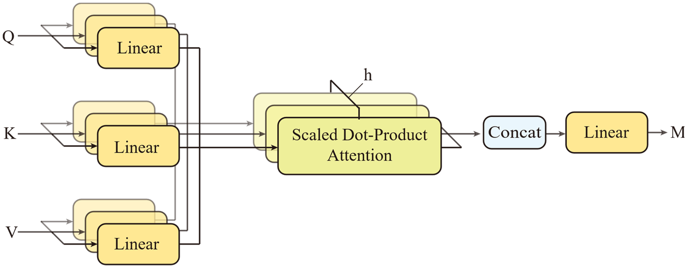
{\begin{aligned} MultiHead (Q, K, V) = Concat ({head}_{1}, {head}_{2}, \dots, {head}_{h}) W^{O} \\ {head}_{i} = Attention (Q W_{i}^{Q}, K W_{i}^{K}, V W_{i}^{V}) \end{aligned}

(2)

where the projection is expressed as parameter matrices

W_{i}^{Q} \in R^{d_{model} \times d_{k}}

W_{i}^{K} \in R^{d_{model} \times d_{k}}

W_{i}^{V} \in R^{d_{model} \times d_{v}}

and

W_{i}^{O} \in R^{h d_{v} \times d_{model}}

Figure 1.

Illustration of the calculation process of the multi-head attention mechanism.

Operational principle of vision transformer algorithm

The operational principle of the Vision Transformer algorithm for image classification is illustrated in Figure 2,¹⁹ and it includes the following steps: (1)

Data processing

Figure 2.

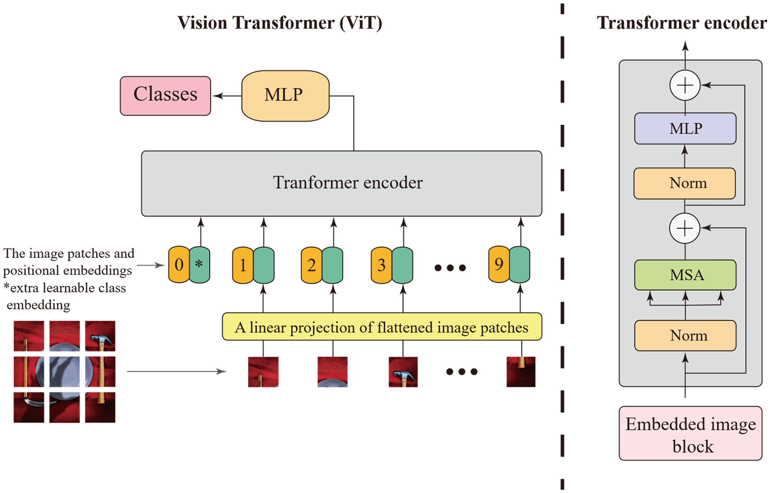
The schematic diagram of the vision transformer algorithm.

The input original image data $X \in R^{H \times W \times C}$ is segmented into multiple patches $X_{p} \in R^{N \times (P^{2} \times C)}$ , where H is the image height, W is the image width, P is the image block's size, C is the number of channels and $N = H W / P^{2}$ is the number of image blocks; (2)

Image block conversion into Transformer encoder input

The two-dimensional image blocks obtained through image segmentation are flattened to obtain a one-dimensional vector, which is then mapped by a trainable linear projection to obtain an embedded image block sequence. In Figure 2, the green blocks adjacent to the orange blocks, numbered 1–9, denote small patch embedding blocks in the sequence; the orange blocks are position embedding blocks that retain the position information on the blocks.

Next, an extra learnable class embedding is added to the embedded image block sequence header.

A sequence of embedding vectors consisting of image block embedding, extra learnable class embedding and position embedding is used as input to the encoder, as shown in equation (3); (3)

Transformer encoding

The encoder used in this study consists of a MSA layer and a fully connected layer (MLP). The output of the multi-head attention layer is given by equation (4), and the MLP output is expressed by equation (5). The input of each layer has a normalised layer (Norm), and the output of each layer applies residual connections; (4)

Output image classification

The extra learnable class embedding (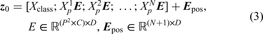 $z_{0}^{0} = X_{class}$ ) is obtained from the state at the Transformer encoder's output ( $z_{L}^{0}$ ), and then the MLP outputs the probability for each class to which the image belongs. The class with the highest probability is taken as the predicted image class, as shown in equation (6).

\begin{matrix} \begin{matrix} z_{0} = [X_{class}; X_{p}^{1} E; X_{p}^{2} E; \dots; X_{p}^{N} E] + E_{pos}, \\ E \in R^{(P^{2} \times C) \times D}, E_{pos} \in R^{(N + 1) \times D} \end{matrix} \end{matrix}

(3)

{z^{'}}_{l} = MSA (LN (z_{l - 1})) + z_{l - 1}, l = 1 \dots L

(4)

\begin{matrix} z_{l} = MLP (LN ({z^{'}}_{l})) + {z^{'}}_{l}, l = 1 \dots L \end{matrix}

(5)

\begin{matrix} y = MLP (z_{L}^{0}) \end{matrix}

(6)

where E indicates the image block embedding information; E _pos denotes the position embedding information; z₀ is the encoder embedding; z_l is the output of MLP at layer l, D is the dimension of data obtained through the linear projection of image blocks by the convolution layer; N is the number of image blocks; L is the number of Transformer encoder layers; y is the image class probability distribution vector.

Improved vision transformer regression algorithm

Based on the Vision Transformer algorithm, this study develops an improved Vision Transformer algorithm for numerical data regression named ViTNR. The block diagram and operational principle of the proposed algorithm are shown in Figure 3.

Figure 3.

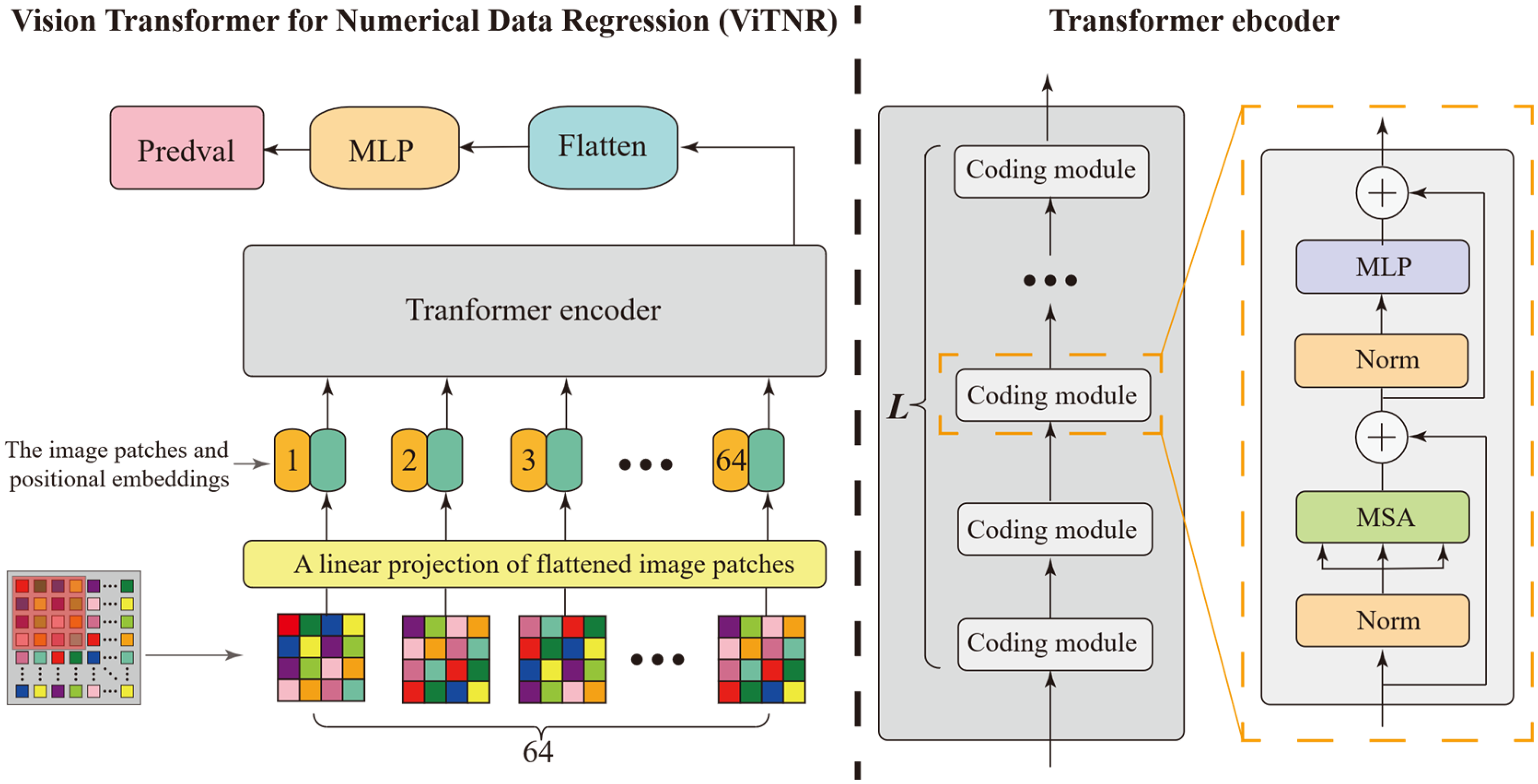
The block diagram and operational principle of the vision transformer numerical regression (ViTNR) algorithm.

The main steps of the ViTNR algorithm include:

The numerical input features are inserted into the two-dimensional array based on the image size, filling the rows first and then columns until all positions of the image are filled to generate two-dimensional image data $X \in R^{H \times W \times C}$ , as illustrated in Figure. 4. The larger the height and width of an image are, and the greater the number of channels is, the more effectively numerical feature data will be used, which is beneficial for improving the model's accuracy. However, if an image size or the number of channels is too large, the model's training time will increase. For the temperature prediction problem of an IH outlet setting strip, the feature number is 10, the number of available channels is one, and (H, W) is (32, 32);

The generated image data are segmented into $4 \times 4$ small image blocks and flattened. A sequence of embedded image blocks is generated through trainable linear projection mapping, which is combined with positional embedding and used as input to the encoder. The sequence vector of image blocks is shown in z₀ defined in equation (7);

The transformer encoder contains L coding modules, each of which includes the MSA layer and the MLP layer. The input of each layer has a normalised layer (Norm), and the output of each layer applies residual connections;

The output module contains the Flatten layer and the MLP. After dimensionality reduction of the Transformer encoder's output data by the Flatten layer, the predicted value (Predval) of output target features obtained by the MLP's output node 1 is determined, as expressed by equation (8).

\begin{matrix} \begin{matrix} z_{0} = [X_{p}^{1} E; X_{p}^{2} E; \dots; X_{p}^{N} E] + E_{pos}, \\ E \in R^{(P^{2} \times C) \times D}, E_{pos} \in R^{N \times D} \end{matrix} \end{matrix}

(7)

\begin{matrix} y = MLP (Flatten (z_{L})) \end{matrix}

(8)

Figure 4.

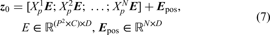
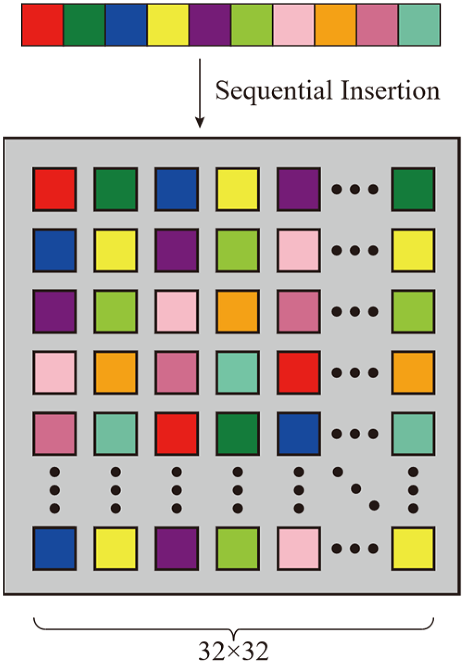
Illustration of data processing.

Model hyperparameter optimisation and settings

The main hyperparameters of the ViTNR model include: Image size, patch size, iteration number (i.e., the number of epochs), batch size, optimiser type, optimiser learning rate, weight decay rate (the AdamW optimiser only), impulse (the SGD optimiser only), a number of coding blocks, the MLP size, the dropout rate of the MLP, the image block mapping dimension (D denotes the number of dimensions of flattened patches), a number of attention heads and the dropout rate of the MSA of multiple attention layers.

Seven hyperparameters, including the optimiser type, a batch size, an optimiser's learning rate, the number of coding blocks, the MLP size, D dimensions of flattened patches and the number of attention heads, are adjusted in this study. The remaining hyperparameters are kept fixed, including the image size of 32, the patch size of four, the weight attenuation (the AdamW optimiser only) of 0.01, the impulse (the SGD optimiser only) of 0.9, the dropout rate of the MLP of 0.01 and the dropout rate of the MSA of multiple attention layers of 0.01.

Results and discussion

Results of model parameters adjustment

In order to ensure the training accuracy and generalisation ability of the model, the dataset was divided into training, test and verification sets according to a certain proportion. In order to ensure consistent data distribution among the datasets, the data were divided into 10 layers by a hierarchical sampling method, and then the data of each layer was sub-divided into training, test and verification sets according to the ratio of 60:20:20.

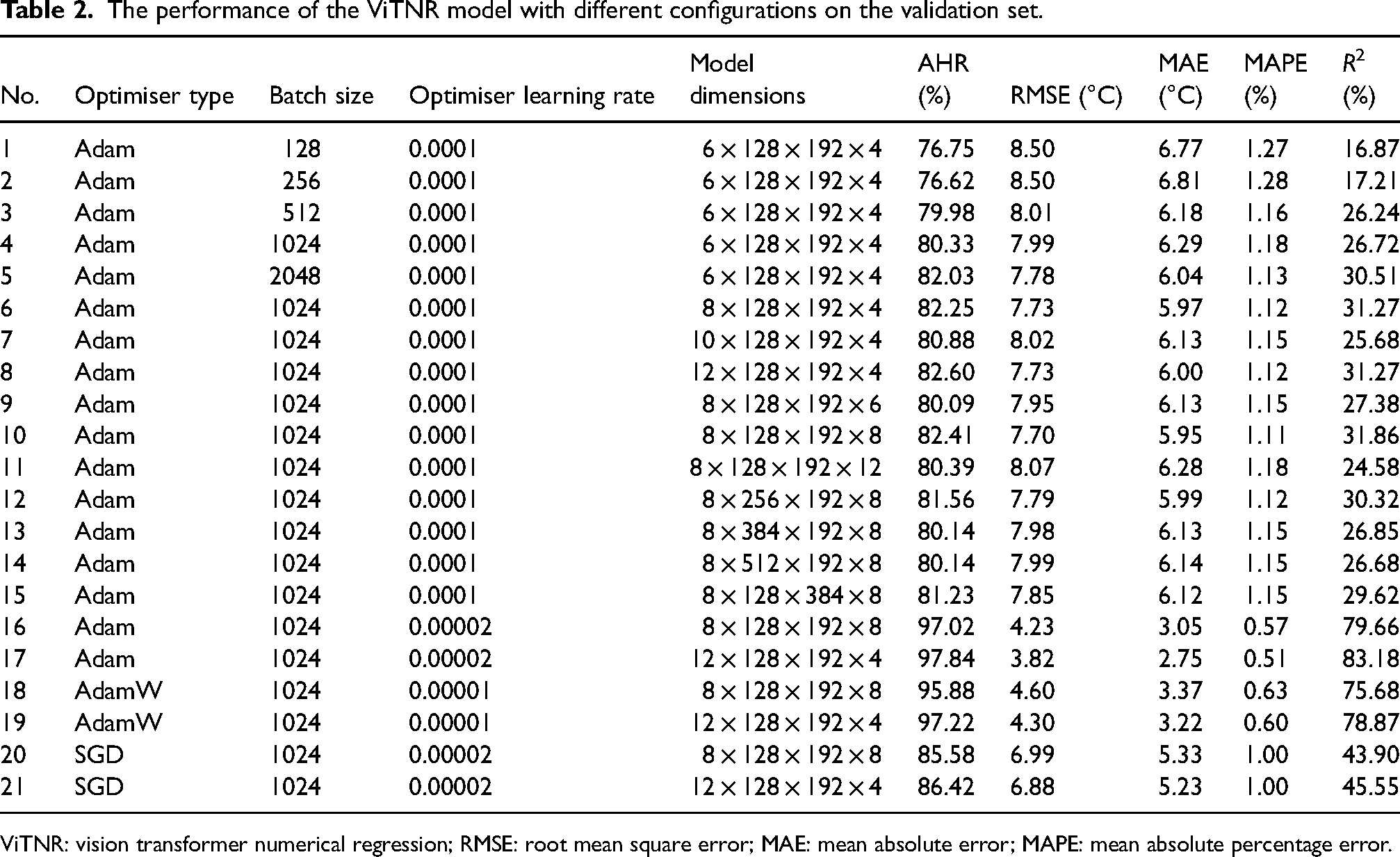
Next, 21 types of hyperparameter combinations of the ViTNR prediction model were optimised during model training on the training dataset, and the model performance for each hyperparameter combination was evaluated on the verification set, as shown in Table 2. The order of Model architecture parameters in Table 2 is as follows: the number of coding blocks, the MLP size, D dimensions of flattened patches and the number of attention heads.

Table 2.

The performance of the ViTNR model with different configurations on the validation set.

No.	Optimiser type	Batch size	Optimiser learning rate	Modeldimensions	AHR(%)	RMSE (°C)	MAE(°C)	MAPE(%)	R²(%)
1	Adam	128	0.0001	6 × 128 × 192 × 4	76.75	8.50	6.77	1.27	16.87
2	Adam	256	0.0001	6 × 128 × 192 × 4	76.62	8.50	6.81	1.28	17.21
3	Adam	512	0.0001	6 × 128 × 192 × 4	79.98	8.01	6.18	1.16	26.24
4	Adam	1024	0.0001	6 × 128 × 192 × 4	80.33	7.99	6.29	1.18	26.72
5	Adam	2048	0.0001	6 × 128 × 192 × 4	82.03	7.78	6.04	1.13	30.51
6	Adam	1024	0.0001	8 × 128 × 192 × 4	82.25	7.73	5.97	1.12	31.27
7	Adam	1024	0.0001	10 × 128 × 192 × 4	80.88	8.02	6.13	1.15	25.68
8	Adam	1024	0.0001	12 × 128 × 192 × 4	82.60	7.73	6.00	1.12	31.27
9	Adam	1024	0.0001	8 × 128 × 192 × 6	80.09	7.95	6.13	1.15	27.38
10	Adam	1024	0.0001	8 × 128 × 192 × 8	82.41	7.70	5.95	1.11	31.86
11	Adam	1024	0.0001	8 × 128 × 192 × 12	80.39	8.07	6.28	1.18	24.58
12	Adam	1024	0.0001	8 × 256 × 192 × 8	81.56	7.79	5.99	1.12	30.32
13	Adam	1024	0.0001	8 × 384 × 192 × 8	80.14	7.98	6.13	1.15	26.85
14	Adam	1024	0.0001	8 × 512 × 192 × 8	80.14	7.99	6.14	1.15	26.68
15	Adam	1024	0.0001	8 × 128 × 384 × 8	81.23	7.85	6.12	1.15	29.62
16	Adam	1024	0.00002	8 × 128 × 192 × 8	97.02	4.23	3.05	0.57	79.66
17	Adam	1024	0.00002	12 × 128 × 192 × 4	97.84	3.82	2.75	0.51	83.18
18	AdamW	1024	0.00001	8 × 128 × 192 × 8	95.88	4.60	3.37	0.63	75.68
19	AdamW	1024	0.00001	12 × 128 × 192 × 4	97.22	4.30	3.22	0.60	78.87
20	SGD	1024	0.00002	8 × 128 × 192 × 8	85.58	6.99	5.33	1.00	43.90
21	SGD	1024	0.00002	12 × 128 × 192 × 4	86.42	6.88	5.23	1.00	45.55

ViTNR: vision transformer numerical regression; RMSE: root mean square error; MAE: mean absolute error; MAPE: mean absolute percentage error.

In Table 2, Nos. 1–5 indicate different batch sizes. The results showed that larger batch sizes could improve the prediction accuracy of the ViTNR model. However, when the batch size increased from 1024 to 2,048, the model training speed became extremely slow. After balancing the training efficiency, the optimal batch size was set to 1024.

Further, Nos. 6–15 indicate different model structures. The two better-performing model structures (i.e., Nos. 8 and 10) were selected as candidates for further model optimisation.

Finally, Nos. 16–21 corresponded to different optimisers used in the model optimisation process. The results showed that the optimal learning rate depended on the optimiser type. The models corresponding to Nos. 16–19 performed better than those corresponding to Nos. 20 and 21; namely, the Adam and AdamW optimisers outperformed the SGD optimiser.

The comparison results showed that the optimal model configuration was No. 17, with the Adam optimiser, a batch size of 1,024, an optimiser learning rate of 0.00002, a number of coding blocks of 12, the MLP size of 128, D = 192 dimensions of flattened patches and a number of attention heads of four. For this hyperparameter combination, all evaluation indexes of the model on the verification set were better than those of the model trained under other hyperparameter combinations.

Comparison models

The DNN represents an artificial neural network that learns complex patterns by stacking multiple layers of neurons, including input, hidden, and output layers.¹⁴ The input layer is responsible for receiving the raw data and passing it to the hidden layer, where, typically, each node represents a feature. The hidden layer is composed of several layers of neurons, which are connected by weights. The function of the hidden layer is to learn and abstract the input data's features in a layer-by-layer manner and perform nonlinear transformations so that the neural network can effectively learn complex relationships in data. The output layer receives the processing results of the hidden layer and uses them to generate the final predicted results based on the specific task requirements.

The CNN consists of a convolutional layer, a pooling layer, an activation function and a fully connected layer. In Wang et al.,²⁴ the author proposed four types of CNN structures equipped with the inception module to address the problem of the plate shape defects in cold-rolled strip steel and used the feature extraction capability of the model to predict the steel strip's flatness. The core idea of the Inception module is to capture features of different sizes through parallel convolutional operations and pooling operations, thereby improving the expressiveness of the network. The core of the convolution layer is the convolution kernel, which represents a small learnable weight matrix that slides over the input image through convolution operations to extract local features. The convolution operation performs a weighted summation and biasing on each local region and then conducts a nonlinear transformation through the activation function, yielding a feature map. The pooling layer is used to downsample the feature maps output by the convolutional layer. It typically retains important feature information through the maximum or average pooling operation while reducing the feature maps’ spatial size, thus reducing the computation burden. By stacking multiple convolution and pooling layers, the size of the feature map can be gradually reduced, and more and more abstract high-level features can be extracted. Finally, through the flattening operation, the high-dimensional feature graph is flattened into a one-dimensional vector, which is then input to the fully connected layer for weighting processing, and the final prediction result is generated by the activation function.

The multi-scale CNN model²⁵ represents an improved CNN. By using multiple convolution kernels of different sizes to conduct convolution operations on the same input image in parallel, this model can focus on feature information of different scales simultaneously, which enhances its perception and feature extraction capabilities. Namely, a more comprehensive and rich feature representation can be obtained by combining multiple feature maps extracted using convolution kernels of different sizes. The merged feature map undergoes a series of convolution, pooling, activation and fully connected operations to obtain the final prediction result.

In Li et al.,¹⁷ the authors proposed the CNPMP model for predicting the mechanical properties of hot-rolled strip steel. This model consists of two parallel branches, as shown in Figure 5. In Branch 1, one-dimensional numerical data are first converted into two-dimensional data through padding and then used as input to the inception module. The inception module processes the same input using convolutional kernels of different sizes, thus aggregating features at different scales. After passing through multiple inception modules, the output image is processed by convolutional layers (Cov1 and Cov2) and a fully connected layer (FC1), finally generating a feature vector. Branch 2 processes the one-dimensional numerical data directly and includes a fully connected layer (FC2), generating a vector. The feature vectors output by the two branches are concatenated to form a comprehensive feature vector, which allows the model to simultaneously fuse image features and numerical data during the feature extraction process, thus enhancing the model's expressive power. Finally, after the data have been processed by a fully connected layer (FC3), the model outputs the final prediction result.

Figure 5.

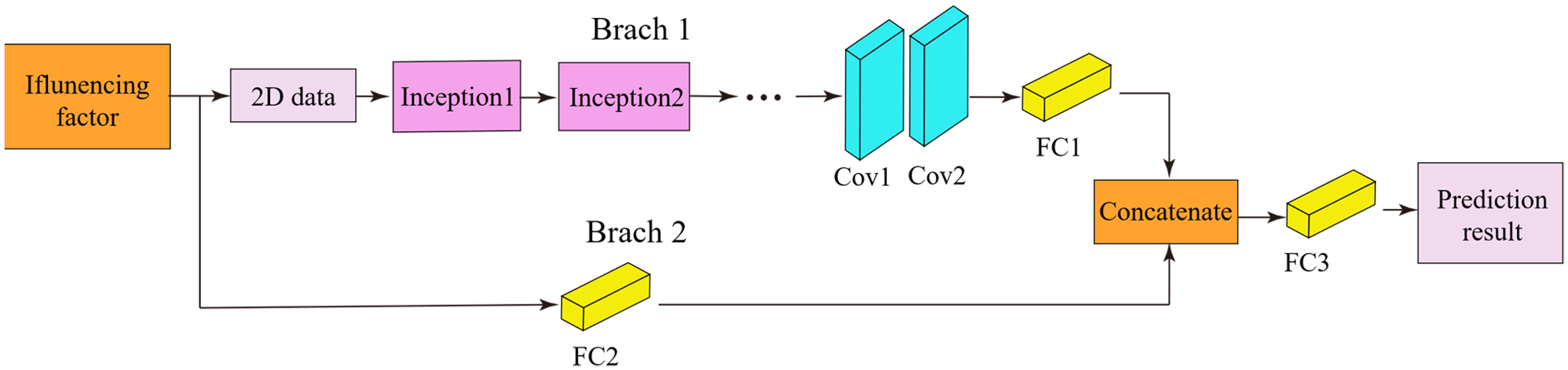
The block diagram of the convolutional network for predicting mechanical properties (CNPMP) algorithm.

The AdaBoost²⁶ is a weighted ensemble learning method that belongs to the boosting class of algorithms, and its block diagram is shown in Figure 6. The core idea of boosting is to train multiple weak learners sequentially and combine their outputs by weighted aggregation to enhance the model's predictive performance. Following this idea, the AdaBoost adjusts the sample weights so that each new weak learner in each round focuses primarily on the samples with larger errors from the previous round of training, which gradually reduces the model's overall error. The specific process is as follows. First, equal weights are assigned to each sample in dataset D, resulting in the initial dataset D1. Then, weak learner 1 is trained using dataset D1, and the sample weights are adjusted based on the error of weak learner 1, yielding dataset D2. Next, weak learner 2 is trained using dataset D2, and the sample weights are adjusted again. This iterative process continues with the training of multiple weak learners. Finally, by combining the outputs of multiple weak learners with weighted aggregation, a strong learner is formed.

Figure 6.

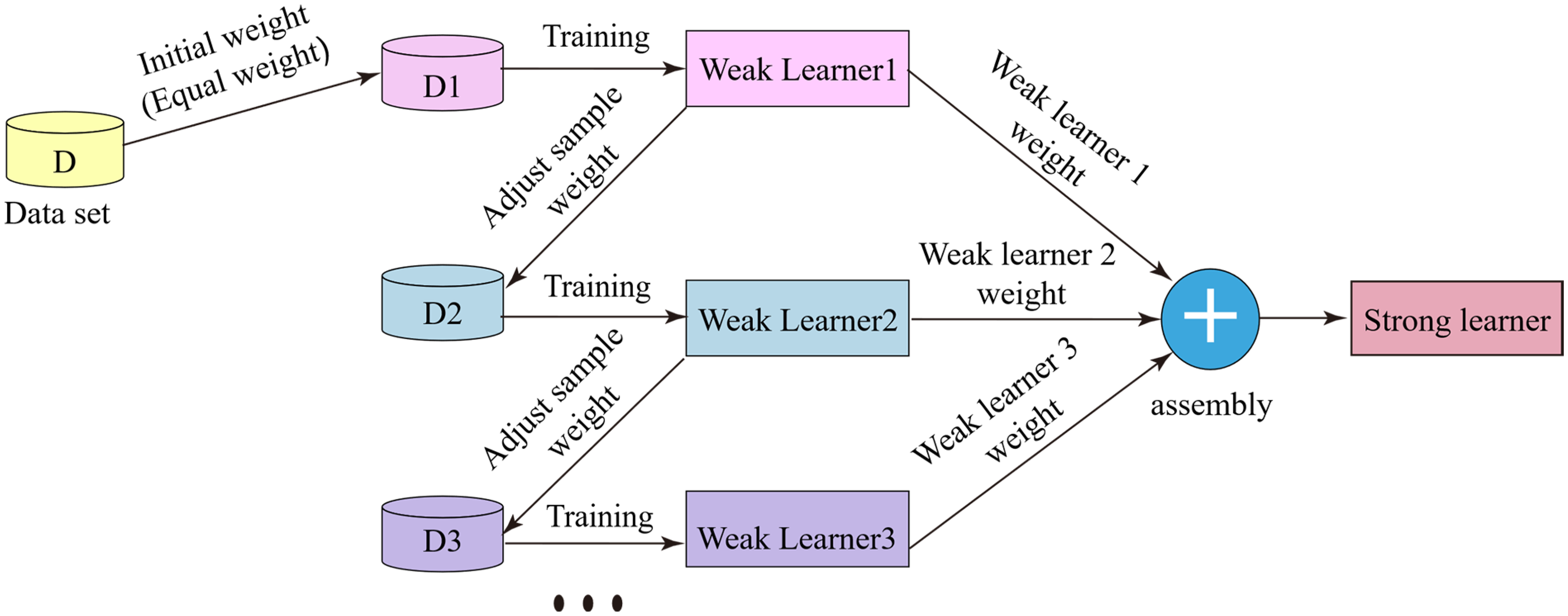
Illustration of the operational principle of the AdaBoost algorithm.

The GBDT is an ensemble learning method based on gradient boosting.¹² It belongs to the Boosting-type algorithms, but unlike the traditional AdaBoost algorithm, the core idea of the GBDT method is to optimise the loss function progressively and use gradient information to guide the training of weak learners. Specifically, in each iteration, the GBDT first calculates the residuals of the current model (i.e., the difference between the current predictions and the true values) and then trains a new weak learner (typically a decision tree) to fit these residuals. This means that each new weak learner aims to ‘correct’ the errors of the previous model, particularly focusing on improving the parts with larger residuals. Finally, the GBDT combines the outputs of all weak learners through weighted aggregation to obtain the final strong learner. Through such a step-by-step adjustment and improvement process, the GBDT can significantly enhance the prediction accuracy of the model.

The RF²⁷ is an ensemble learning-based algorithm, which randomly extracts multiple sub-datasets from the original dataset by the bootstrap method and then uses the obtained sub-datasets to train multiple decision trees in parallel and finally either votes or averages their prediction results to improve the accuracy and stability of the model.

The core idea of the KNN algorithm²⁸ is to classify or perform the regression on distance between samples. Unlike many other algorithms, the KNN algorithm does not learn during the training phase but stores all training samples directly in memory. In the prediction stage, the KNN algorithm calculates the distance between the sample to be predicted and all the training samples and makes a prediction based on the nearest K neighbours. In the regression task, the KNN algorithm obtains the final prediction by calculating the average value of the KNNs.

The SVM¹³ is a supervised learning algorithm for classification and regression, whose main goal is to improve the generalisation ability of a prediction model by finding an optimal hyperplane in the feature space, thus separating the data points as far as possible while maximising the spacing. For regression tasks, the SVM finds a regression plane that maximises the interval so that most data points are located near the plane while maintaining a certain tolerance. The SVM determines the position of the regression plane by focusing on the support vector located on the boundary data. For nonlinearly separable data, the SVM uses kernel functions to map the data to a higher-dimensional feature space, where linear separability is realised to handle complex regression tasks.

Prediction results analysis

The 3664 data samples from the test dataset were fed to the ViTNR model with the optimal configuration (3,000, Adam, 1,024, 0.00002, 12 × 128 × 192 × 4) for evaluation. The evaluation indexes included the AHR, RMSE, MAE, MAPE and R². On the test dataset, the ViTNR model achieved the AHR, RMSE, MAE, MAPE and R² values of 97.37%, 3.922, 2.788 °C, 0.521% and 81.75%, respectively.

The DNN model consisted of five hidden layers, each of which contained 50 nodes, the L2 regularisation parameter was 0.1, the activation function was the ReLU function and the initial learning rate was set to 0.0001. The CNN model²⁴ adopted the Model C framework, the Adam optimiser and a learning rate of 0.0005. The multi-scale CNN model²⁵ included the inception module with two types of asymmetric convolution kernels, input feature reuse, Adam optimiser and a 0.0005 learning rate. The CNPMP model¹⁷ had a simplified Inception module that was stacked and spliced; the selected optimiser was the AdamW optimiser, the weight decay coefficient was 0.01 and the learning rate was set to 0.0001.

The five shallow learning-based contrast models were the AdaBoost, GBDT, KNN, SVM and RF models. The optimal hyperparameter combination of the GBDT model was as follows: a learning rate was 0.11, an estimator was 700 and the maximum depth was nine. The optimal hyperparameter combination of the KNN model was: the number of neighbours was two, and weights denoted distances. The optimal hyperparameter combination of the SVM model was: C = 19 and epsilon = 0.11. The optimal hyperparameter combination of the RF model was as follows: The number of estimators was 800, the maximum depth was 80 and the minimum sample split was two. The optimal hyperparameter combination of the AdaBoost model was: learning rate = 0.11, estimator = 800 and max depth = 13. Both the TPE algorithm and the DE algorithm were used to optimise the shallow learning-based models and obtain optimal results.

The simplified model of the IH outlet setting strip temperature of continuous hot galvanizing line (CGL) denoted a linear equation of alloying points, coating target thickness and unit line speed, where the alloying points were related to the steel class.

The accuracy indexes of the ViTNR model, comparison models and simplified production site model on the test dataset are shown in Table 3. In Table 3, AHR is the hit rate of the IH outlet setting strip temperature prediction error within 10 °C, which represents the main accuracy evaluation index of a model in the production field; RMSE represents the standard deviation between the predicted and actual values; MAE is the average value of the absolute error between the predicted and actual values; MAPE is the average of the absolute error between the predicted and actual values, expressed as a percentage of the true value; the R² value measures the goodness of fit of the model to the data, reflecting the proportion of the variance of the dependent variable that the model explains.

Table 3.

The accuracy comparison results of different models on the test dataset.

Model	AHR (%)	RMSE (°C)	MAE (°C)	MAPE (%)	R² (%)
Proposed ViTNR	97.37	3.92	2.79	0.52	81.75
CNPMP	93.25	5.43	4.12	0.77	66.07
DNN	92.78	5.53	4.04	0.76	63.33
CNN	88.23	6.77	5.48	1.02	47.41
Multi-scale CNN	87.46	6.70	5.36	1.01	48.09
AdaBoost	96.91	4.05	2.63	0.49	80.55
GBDT	96.63	4.11	2.76	0.52	79.94
KNN	96.03	4.28	2.05	0.38	78.25
RF	96.02	4.24	2.76	0.52	78.40
SVM	92.70	5.83	4.47	0.84	59.14
simplified model of CGL	35.88	21.02	17.08	3.35	0.20

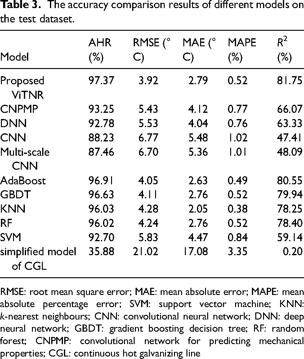
RMSE: root mean square error; MAE: mean absolute error; MAPE: mean absolute percentage error; SVM: support vector machine; KNN: k-nearest neighbours; CNN: convolutional neural network; DNN: deep neural network; GBDT: gradient boosting decision tree; RF: random forest; CNPMP: convolutional network for predicting mechanical properties; CGL: continuous hot galvanizing line

As shown in Table 3, among all models, the CNPMP model (which denoted a deep learning-based model) had the highest AHR index, the AdaBoost model (which indicated a shallow learning-based model) had the highest AHR index, and the KNN model had the lowest MAE value. The measured and predicted values of the proposed ViTNR model and these three models are shown in Figure 7.

Figure 7.

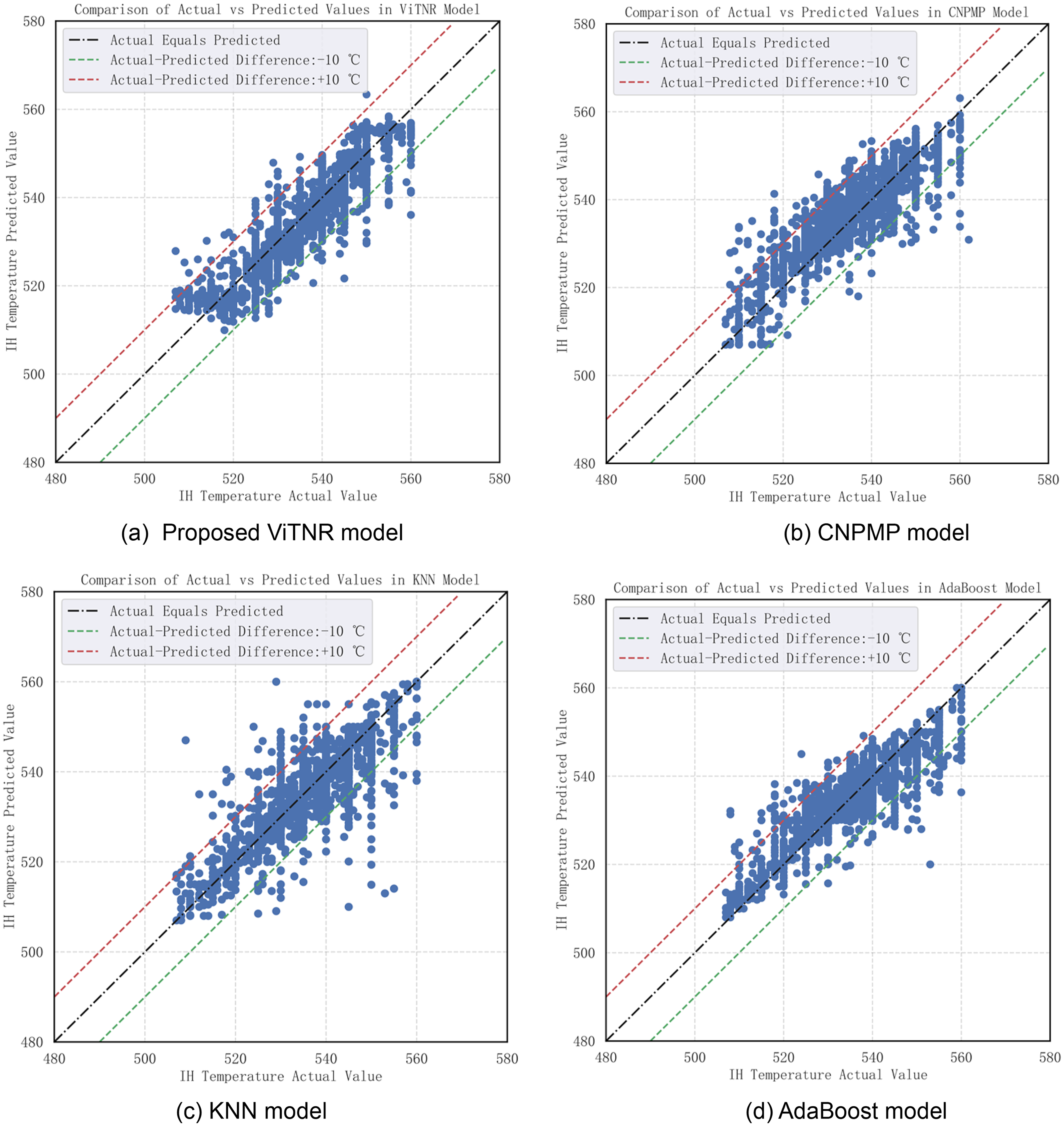
The scatter plots of the actual value versus the predicted value of different prediction models on the test dataset.

Model accuracy comparison results

The index in Table 3 represents the accuracy index of a prediction model on the test dataset, but the data of the test set were not used in model training. Therefore, the accuracy of the model on the test set could reflect both the accuracy of the model on the test set and the prediction ability of the model on unknown data, which is also known as the generalisation ability.

Based on the comparison results in Table 3 and Figure 7, the following conclusion could be drawn:

The AHR, RMSE and R² indexes of the ViTNR model were 97.37%, 3.92 °C and 81.75%, respectively, which denoted the optimal result among all models. The AHR, RMSE and R² values of the AdaBoost model were 96.91%, 4.05 °C and 80.55%, respectively, following those of the ViTNR model. Thus, the proposed ViTNR model outperformed the AdaBoost model by 0.46%, 0.13°C and 1.20% on the AHR, RMSE and R² indexes, respectively, indicating that the ViTNR model had high accuracy and strong generalisation ability;

The MAE and MAPE indexes of the KNN model were 2.05 °C and 0.38%, respectively, which denoted the best results among all models. The MAE and MAPE values of the KNN model were 0.74 °C and 0.14% lower than those of the ViTNR model, respectively; however, the RMSE value of the KNN model was higher than that of the ViTNR model. This indicated that the variance of the prediction error of the KNN model was large, that is, the prediction result fluctuated significantly. Figure 7 showed that the data points of the ViTNR model (Figure 7(a)) were close to the diagonal and evenly distributed, whereas the data points of the KNN model (Figure 7(c)) were loosely distributed with more extreme error points;

The parameters of alloying points in the simplified model of the current CGL were closely related to the steel grade. When the types of steel were few, the simplified model could achieve higher accuracy and meet the production requirements. However, due to the wide variety of steel grades and addition of new steel grades, accurately determining the alloying points was challenging, which led to lower prediction accuracy of the simplified model showed by the indicators listed in Table 3. As a result, the simplified model did not meet the IH outlet setting strip temperature control requirements, and a more accurate model is needed as an alternative.

Conclusion

This study proposes the ViTNR model that transforms numerical features into images by the filling method and uses segmented images as input for deep learning. The multi-head attention mechanism of the Transformer encoder is used to learn the importance of input feature information, thus improving the model's accuracy.

In addition, based on the proposed ViTNR model and the production data with good alloying quality, combined with hyperparameter adjustment, this study designs a ViTNR prediction model for the temperature of a hot-dip galvanised IH outlet setting strip. The comparison results show that the AHR, RMSE and R² indexes of the ViTNR model are the best among all comparison models. Moreover, the ViTNR model has the advantages of high prediction accuracy, strong generalisation ability and small prediction error fluctuations.

On the basis of good prediction performance of ViTNR offline modelling, an online prediction program of IH outlet setting strip temperature will be developed for replacing the present simplified model of CGL, the online prediction accuracy of ViTNR model by comparing the prediction values of ViTNR model and the IH outlet strip temperature setting control values of CGL will be evaluated, and the model will be improved progressively by continuously gathering new production data and model optimisation for IH outlet strip temperature setting control.

Footnotes

Declaration of conflicting interests

The authors declared no potential conflicts of interest with respect to the research, authorship, and/or publication of this article.

Funding

The authors disclosed receipt of the following financial support for the research, authorship, and/or publication of this article: This study was supported by the Science and Technology Project of Fujian Province (grant number, 2018H0015).

Research

Mechanics and control of metallurgical equipment, Intelligent manufacturing of metallurgical industry process, Intelligent theory and application of industrial big data.

ORCID iDs

Wei Wang

Ziang Wang

References

Bian

. Development of hot dip galvanized steel strip and its application in automobile industry. J Iron Steel Res Int 2006; 13: 47–50.

Dey

Sahu

Banerjee

, et al. A review on metallurgical features of hot-dip aluminized steel. Eng Res Exp 2023; 5: 012002.

Dallin

. Continuous hot-dip galvanizing—process and products. Galvinfo Center—A Program of the International Zinc Association, Galvanizing-2015 2015; 8–20.

Chuan

Yonglin

Huaxiang

. Effect of galvannealing temperature on microstructure and properties of coating on galvannealed high strength IF steel. Trans Mater Heat Treat 2014; 35: 79–83.

Sanming

Biao

. Analysis of the factors affecting the galvannealing process of alloying hot dip galvanized steel sheet. Baosteel Technol 1998; 16: 34–37.

Liu

Zhou

, et al. A machine learning and genetic algorithm-based method for predicting width deviation of hot-rolled strip in steel production systems. Inf Sci (Ny) 2022; 589: 360–375.

Dong

Luan

, et al. Prediction and analysis of key parameters of head deformation of hot-rolled plates based on artificial neural networks. J Manuf Process 2022; 77: 282–300.

Mao

Yang

Huang

, et al. Coating Thickness Modeling and Prediction for Hot-dip Galvanized Steel Strip Based on GA-BP Neural Network[C]//2020 Chinese Control And Decision Conference (CCDC). Hefei, China: IEEE, 2020, 3484–3489.

Kai

Lei

Yuqiang

, et al. Deep learning: yesterday, today, and tomorrow. J Comput Res Dev 2013; 50: 1799–1804.

10.

Feiyan

Linpeng

Jun

. Review of convolutional neural network. Chin J Comput 2017; 40: 1229–1251.

11.

Yifeng

. Pedestrian detection based on deep learning by shallow learning. Wuhan, China: Wuhan University, 2016.

12.

Luxi

Dianyao

Baoqian

, et al. Prediction of strip running speed in cooling zone after rolling based on gradient boosting algorithm. Metall Ind Autom 2023; 47: 62–69+99.

13.

Yuan

Yali

, et al. Establishment and Optimization of Gas Flow Prediction Model for Annealing Furnace Based on GA-SVM[C]//2018 37th Chinese Control Conference (CCC). Wuhan: IEEE, 2018, 3486–3490.

14.

Xie

Suvarna

, et al. Online prediction of mechanical properties of hot rolled steel plate using machine learning. Mater Des 2021; 197: 109201.

15.

Zhou

Tian

, et al. Prediction of mechanical properties of hot rolled strips with generalized RBFNN and composite expectile regression. IEEE Access 2022; 10: 106534–106542.

16.

Liu

Zhang

. Mechanical properties prediction for hot rolled alloy steel using convolutional neural network. IEEE Access 2019; 7: 47068–47078.

17.

Xie

Zhao

, et al. Prediction model for mechanical properties of hot-rolled strips by deep learning. J Iron Steel Res Int 2020; 27: 1045–1053.

18.

Vaswani

Shazeer

Parmar

, et al. Attention Is All You Need[M]. arXiv, 2023.

19.

Dosovitskiy

Beyer

Kolesnikov

, et al. An Image is Worth 16(16 Words: Transformers for Image Recognition at Scale[M]. arXiv, 2021.

20.

Pokorny

Kolisko

Balik

, et al. Reaction kinetics of the formation of intermetallic Fe–Zn during hot-dip galvanizing of steel. Metalurgija 2016; 55: 111–114.

21.

Bicao

Jianhua

Xuping

, et al. Effects of zinc bath temperature on the coatings of hot-dip galvanizing. Surf Coat Technol 2008; 202: 1785–1788.

22.

Yong

Taixiong

. Influence factors of powdering-resistance of galvannealed steel sheets. Corros Prot 2012; 33: 610–613+629.

23.

Jiashun

Feng

Rendong

, et al. Influence factors on properties and research progress of galvannealed technology. Hot Work Technol 2010; 39: 155–159+162.

24.

Wang

Peng

, et al. Application of convolutional neural networks for prediction of strip flatness in tandem cold rolling process. J Manuf Process 2021; 68: 512–522.

25.

Zhang

Tan

, et al. Controlled cooling temperature prediction of hot-rolled steel plate based on multi-scale convolutional neural network. Metals (Basel) 2022; 12: 1455.

26.

Freund

Schapire

. A decision-theoretic generalization of on-line learning and an application to boosting. J Comput Syst Sci 1997; 55: 119–139.

27.

Breiman

. Random forests. Mach Learn 2001; 45: 5–32.

28.

Cover

Hart

. Nearest neighbor pattern classification. IEEE Trans Inf Theory 1967; 13: 21–27.