





Abstract
Converter steelmaking is a key technology in steel production. Precise prediction of the endpoint carbon content is of great significance for improving steel quality, optimising production efficiency, and reducing costs. In response to the limitations of traditional prediction methods, this study proposes a multi-stage endpoint carbon content prediction model for converter steelmaking based on the grey wolf optimisation (GWO) algorithm and bidirectional long short-term memory (BiLSTM) networks. First, a dynamic cumulative quantity modelling method based on function fitting is employed to divide the steelmaking process into three stages according to CO and CO2 emission volumes. Next, the autoencoder combined with the optuna optimisation algorithm is used to reduce the dimensionality of 2048-dimensional spectral data. Finally, the GWO algorithm is utilised to optimise the parameters of the BiLSTM model. Experimental results demonstrate that compared with back propagation, long short-term memory, BiLSTM and transformer models, the proposed model exhibits relatively lower mean absolute error (MAE), mean absolute percentage error, and root mean square error (RMSE) across all stages of CO and CO2 emission prediction. Especially in the third stage, the prediction errors are significantly reduced. For CO and CO2 gas, the MAE decreases to 18.0017 and 1.7307, respectively, and the RMSE decreases to 20.2151 and 2.1321, respectively. The contributions of various features to the prediction results are clarified through the analysis using the Shapley Additive exPlanations method, thereby enhancing the interpretability of the model. This research provides an efficient and reliable method for the precise prediction of the endpoint carbon content in converter steelmaking, which has important practical significance for optimising the steel-making production process.
Keywords
Introduction
The converter steelmaking process is one of the key technologies in the iron and steel industry, dominating global steel production and accounting for ∼70% of the world's total steel output. 1 Accurately predicting and controlling the carbon content and temperature of molten iron is critical for producing high-quality steel, especially in fields such as bridge construction, road infrastructure, shipbuilding, and aerospace, where the performance requirements for steel are extremely stringent.2–4 Precise control of the endpoint in the converter steelmaking process is essential for ensuring product quality, production efficiency and cost management.5,6
Generally speaking, obtaining the carbon content at the end of converter steelmaking can be divided into contact measurement and non-contact measurement. Sublance detection is the most commonly used method for contact measurement. It involves inserting a probe into the molten steel bath in the converter and using various sensors to obtain information such as the temperature and composition of the molten steel. However, it can only detect the carbon content and temperature of the molten steel at specific time nodes, and the maintenance cost is high. 7 The non-contact methods include manual fire observation, static model and dynamic model control.8–11 The traditional endpoint prediction techniques for converter steelmaking face several limitations. 12 Early manual flame observation relied heavily on the experience of operators, resulting in strong subjectivity and low accuracy. Although static models represented an improvement, they struggled to adapt to the complex and dynamic steelmaking process, leading to significant prediction errors.
In addition to the methods mentioned above, the furnace gas analysis method has certain advantages, as it can be applied to converters of different models. Pan et al. 13 calibrated the flue gas composition and constructed a mathematical model for the continuous prediction of the carbon content and temperature during the blowing process. They also carried out an offline simulation for the actual smelting process of a steel plant in Tangshan. However, this method is only applicable to the end-point control of low-carbon steel grades and has strict requirements for the production site environment.
In traditional converter steelmaking processes, operators determine the endpoint carbon content and temperature by observing characteristics such as the colour and brightness of the flame inside the furnace. Inspired by this practice, and with the continuous advancement of computer technology and data analysis methods, researchers have proposed various approaches to predict the endpoint by extracting features from flame images or spectral data.
Liu et al. 14 utilised a three-dimensional multi-layer complex network to mine the texture features of dynamic flames, and combined dynamic features with static features such as flame colour to construct a prediction model, which improved the end-point carbon content. However, this method only analysed the features of the flame at the furnace mouth and ignored the process data collected during the entire reaction process. Zhou et al. 15 used the information of the steelmaking process contained in the flame spectrum and the furnace mouth image as the input of the model, and constructed a fuzzy support vector machine classification model for the prediction of the end-point carbon content.
However, flame images contain a large amount of information, and the harsh collection environment is prone to interference, which can degrade image quality and damage equipment. Additionally, the complexity of analysis algorithms, challenges in feature extraction, poor adaptability, and high computational resource requirements make it difficult for researchers to achieve real-time prediction of temperature and carbon content in molten steel during the later stages of steelmaking.
In the process of converter steelmaking, the chemical reaction of the material in the furnace will emit a spectrum with a specific wavelength and intensity distribution. Compared to flame images, spectral features can more directly reflect changes in the chemical composition and physical state of the molten steel and are less susceptible to environmental interference.
The change of spectral information can reflect the carbon conversion process, thus indirectly reflecting the change of carbon content. 16 Zhang et al. 17 extracted the main characteristics of the flame spectrum through factor analysis, and developed a non-contact prediction model by using big data deep learning and the CPS framework, which improved the universality of the model. However, this method only extracts the local frequency domain features of the spectral data, resulting in a relatively low prediction accuracy. Zhao et al. 18 used the flame spectrum data at the converter mouth, combined with the rough set attribute reduction algorithm optimised by the baseline estimation and denoising with sparsity (BEADS) algorithm and the genetic algorithm, extracted the features closely related to the carbon content, and used the back propagation (BP) neural network for prediction. The results show that the hit rate of carbon content prediction reaches 94.0%. Shao et al. 19 divided the basic oxygen steelmaking blowing process into four stages, and applied the directed acyclic graph-support vector machine (DAGSVM) model to predict the carbon content of the flame spectrum data. However, the application scenario of this method is limited, and it is only applicable for operators to predict that the carbon content is < 0.5%.
Due to the dynamic changes of spectral feature data, the characteristics and changing trends of data in different stages are significantly different. All the above methods uniformly process the entire process and ignore the errors caused by the characteristics of different stages. In order to more accurately capture the dynamic change characteristics of the converter steelmaking process and improve the prediction accuracy, this paper introduces a method of using the grey wolf optimisation and bidirectional long short-term memory (GWO-BiLSTM) model to predict the carbon content in converter steelmaking. This method first fits the function curves of the emissions of CO and CO2, and divides the entire reaction process into three stages. Then, an autoencoder is used to reduce the dimension of the data of these three stages, respectively, retaining the main features of the spectral information. Subsequently, a GWO-BiLSTM model is constructed to predict the dimension-reduced data, and the Shapley Additive exPlanations (SHAP) method is used to explain the influence degree of each feature in the model on the prediction results.
In summary, the highlights of this study are as follows:
Aiming at the problem that it is difficult to accurately calculate the total emissions of CO and CO2 due to the intermittent sampling of flue gas analysis mass spectrometers, a dynamic cumulative quantity modelling method based on function fitting was proposed. The cumulative emissions were selected as the threshold to divide the converter steel-making process into three stages. The combination of autoencoder and Optuna optimisation method was used to reduce the dimension of 2048-dimensional high-dimensional spectral data. The Bayesian optimisation algorithm of Optuna was utilised to determine the optimal dimension reduction and learning rate, retaining the key information of the spectral data. The GWO algorithm was applied to optimise the parameters of the BiLSTM prediction model for the three stages of the CO and CO2 fitting curves. This enables the BiLSTM model to better capture the trends of time-series data when predicting the changes of CO and CO2, improving the prediction accuracy.
In the ‘Methodology’ section of this study, the model proposed in this study is introduced. In the ‘Case study’ section, the method of dimensionality reduction of spectral data is focused on, and the effect of dimensionality reduction is verified through principal component analysis (PCA). In the ‘Experimental results and discussion’ section, the experimental results are analysed and the effectiveness of the model is verified. Finally, the ‘Conclusions and future work’ section presents the conclusions and future research directions.
Methodology
BiLSTM
Recurrent neural network (RNN) has shown some advantages in processing sequence data, but it faces key problems such as long-term memory loss, gradient disappearance and gradient explosion. To solve these problems, Hochreiter and Schmidhuber 20 proposed a long short-term memory (LSTM) neural network model, which introduces unique memory units and gating mechanisms on the basis of RNN. Through the use of different gate structures as well as neurons, it is able to effectively control the learning rate. By using different gate structures and neurons, it can effectively control the learning rate and forgetting rate, and has the function of memorising long and short-term sequence data.
The LSTM cell consists of an input gate, a forgetting gate, an output gate, and a cell state.
21
The input gate controls the entry of new information into the cell's state by filtering information from the current input and the hidden state of the previous time step. The forgetting gate decides whether the information in the cell state is discarded or not. The output gate decides what information to output as a hidden state to pass to the next time step. The computation process is as follows:






BiLSTM sets two independent hidden layers on top of LSTM and maps to the same output layer spliced for output. Running forward and reverse LSTMs simultaneously at each time step enables simultaneous acquisition of information in both the front and back directions of the sequence. 22 The forward LSTM unit processes the data step-by-step from the start position of the sequence to capture historical information. The reverse LSTM unit processes the data from the end of the sequence to capture future information about the data. In this way, the BiLSTM model can capture the dependencies in the sequence more comprehensively. 23 The principle is shown in Figure 1.
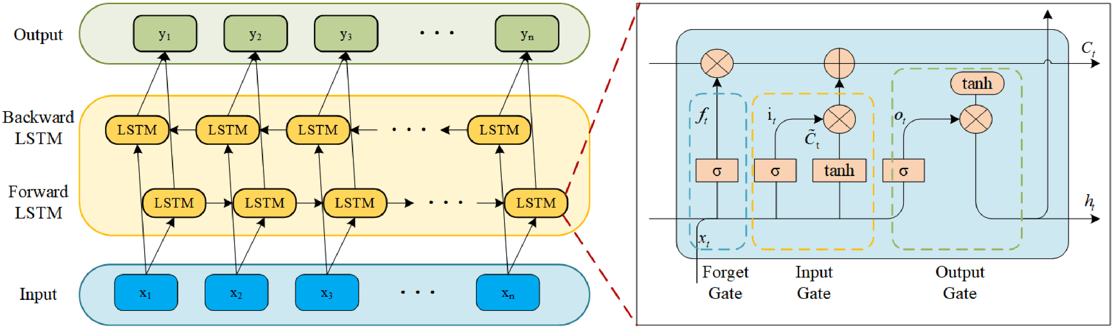
The principle of bidirectional long short-term memory (BiLSTM).
Grey wolf optimisation
The GWO algorithm is a group intelligence optimisation algorithm proposed by Mirjalili in 2014. The GWO algorithm simulates the social hierarchy and hunting strategy of grey wolves, which strikes a good balance between global search and local exploitation to find the optimal solution to the problem. 24
Grey wolf packs have a clear social hierarchy in nature, which is sequentially divided into four classes:
The GWO algorithm analogises the solution space of the problem to be optimised to the search space of a grey wolf, where the location of the prey corresponds to the global optimal solution of the optimisation problem and the location of the grey wolf corresponds to the candidate solution. During the hunting process, the wolves achieve the optimisation objective through three main behaviours: encircling, pursuing and attacking the prey.
Encircle prey. In the GWO algorithm, the grey wolf pack approaches the prey gradually by adjusting its position and the mathematical expression for encircling the prey is as follows:




Pursuit of prey. After encircling the prey, the grey wolf pack adjusts its position according to the prey's direction of movement and gradually approaches the prey. The position information of α, β and δ wolves guides other grey wolves (ω wolves) to update their positions. The distances between grey wolves and α, β and δ wolves are calculated as follows, respectively:

Based on the positions of α, β and δ wolves, the grey wolf updates its own position:


Attacking prey. Grey wolf packs, led by α, β and δ wolves, disperse in pursuit of prey. When the prey stops moving, the grey wolf pack attacks. That is, when the value of is small, the grey wolves move in smaller steps and gradually approach the prey. As shown in the following equation:

Autoencoder
An autoencoder is a neural network-based unsupervised learning model designed to learn effective low-dimensional representations from high-dimensional data. 25 Its core architecture is composed of two parts: an encoder and a decoder. The encoder is responsible for mapping the high-dimensional input data, that is, the spectral data in this study, to a low-dimensional latent space representation. And the decoder performs the opposite operation of the encoder, reconstructing the potential representation into high-dimensional data.
The encoder extracts key features from the spectral data through a series of nonlinear transformations and compresses them into a low-dimensional vector. For spectral data

The decoder reconstructs the low-dimensional representation z into high-dimensional data


GWO-BiLSTM
In this study, a GWO-BiLSTM model is proposed. The process of this model is shown in Figure 2, and the specific steps are as follows:
The USB4000 + fibre optic spectrometer is used to collect 2048-dimensional spectral data and flue gas data. Function fitting is performed on the emissions of CO and CO2, respectively, and they are divided into three stages according to the first derivative. The autoencoder is integrated with the Optuna optimisation algorithm to determine the optimal dimensionality reduction parameters and learning rates for the spectral data across each stage. The encoder projects the high-dimensional spectral features onto a latent space, while the decoder reconstructs the original input. The model is trained via BP to minimise the reconstruction error. The GWO algorithm is employed to search for the optimal hyperparameters of the BiLSTM, including the number of nodes in the hidden layer and the dropout rate. The dataset is divided into a training set and a test set at a ratio of 7:3. The performance of the proposed model is evaluated using mean absolute error (MAE), root mean square error (RMSE) and mean absolute percentage error (MAPE) as evaluation indicators.
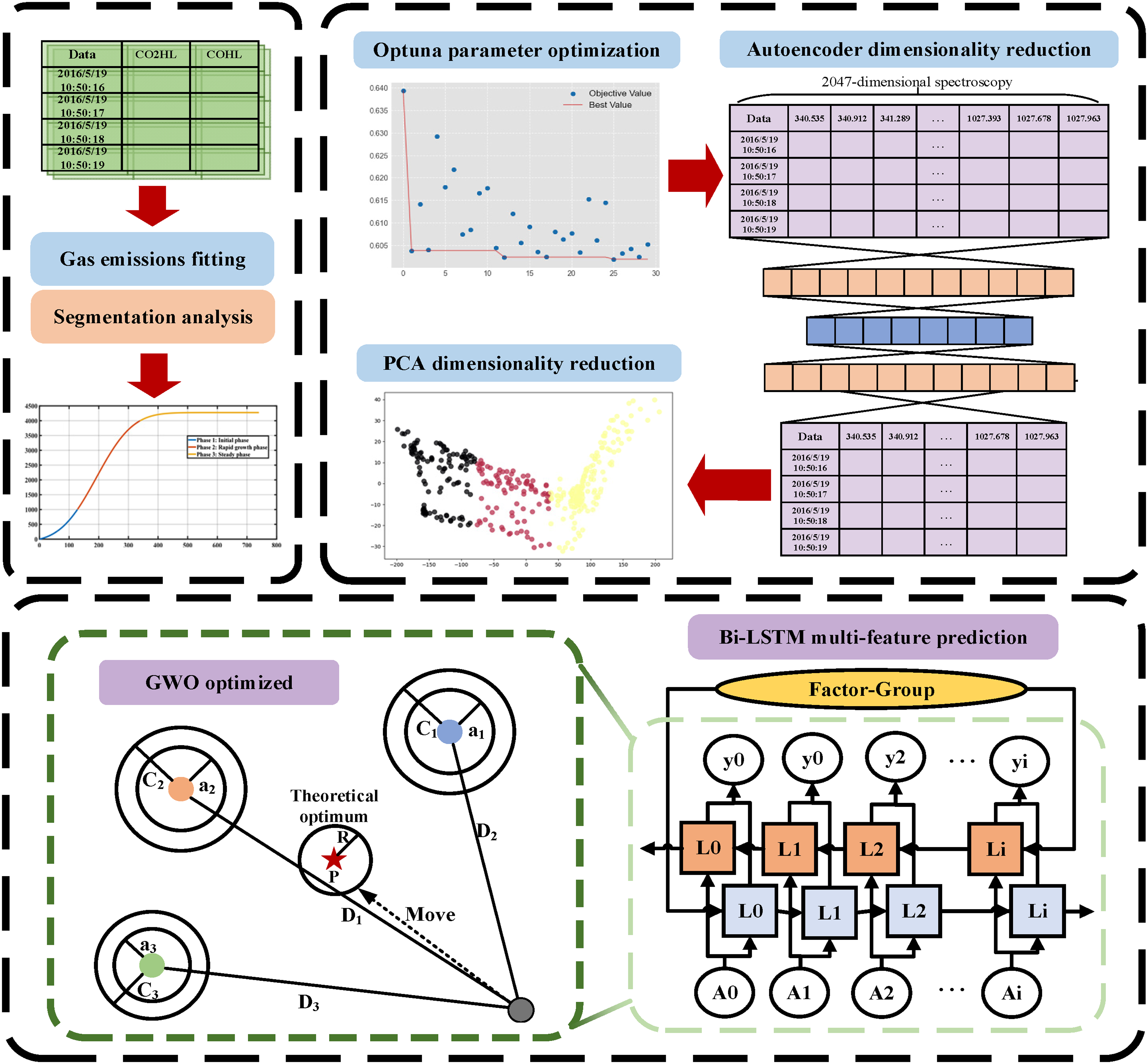
Full-text research framework diagram.
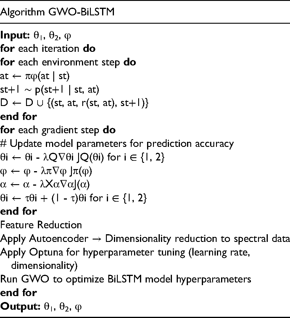
In order to more intuitively demonstrate the construction and training process of the GWO-BiLSTM model, the following is the pseudocode of this model.
Case study
Acquire the furnace mouth
The experimental data is divided into two parts: spectral data and flue gas data. In converter steelmaking, oxygen oxidises various impurities in the hot metal through oxidation reactions. The slag produced by oxidation will float on the surface of molten steel, which plays a role in protecting molten steel, preventing excessive oxidation and adsorbing harmful impurities. In the construction of experimental equipment, based on a 150 kg medium frequency furnace, the converter body is composed of a stainless-steel furnace body section and a furnace mouth section.
Then, a hood is installed above the furnace mouth and a simple water dust removal device is equipped as a flue gas recovery system. A multimode fibre is installed on the right side of the furnace mouth to connect the light microscope probe.
The flame spectrum data is transmitted to the USB4000 + fibre optic spectrometer. The flame spectrum information of the furnace mouth during the whole smelting period is collected and analysed in real time. The wavelength range of the spectrometer is from 300 to 1025 nm, which fully covers the spectral information perceptible to the human eye. The original data are shown in Table 1.
The original flame spectral data.
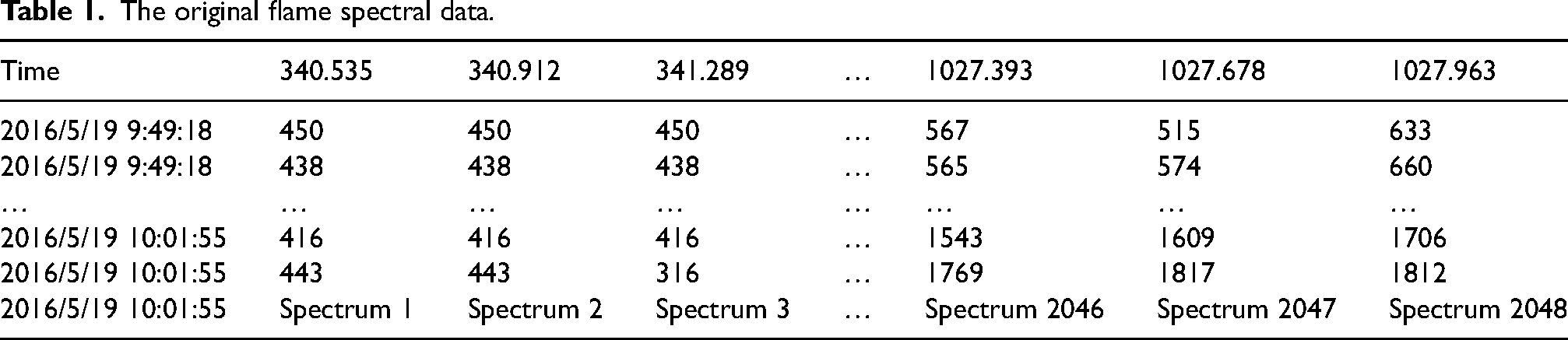
The instrument divides the measurable wavelength into 2048 points according to a fixed step size, that is, the amount of data collected each time is 2048 dimensions, corresponding to the light intensity at each wavelength. With a sampling interval of 0.5 s, two sets of spectral data are collected every second. On average, 3.684 million data points can be obtained throughout the smelting process. The formation process of blast furnace flame is shown in Figure 3.
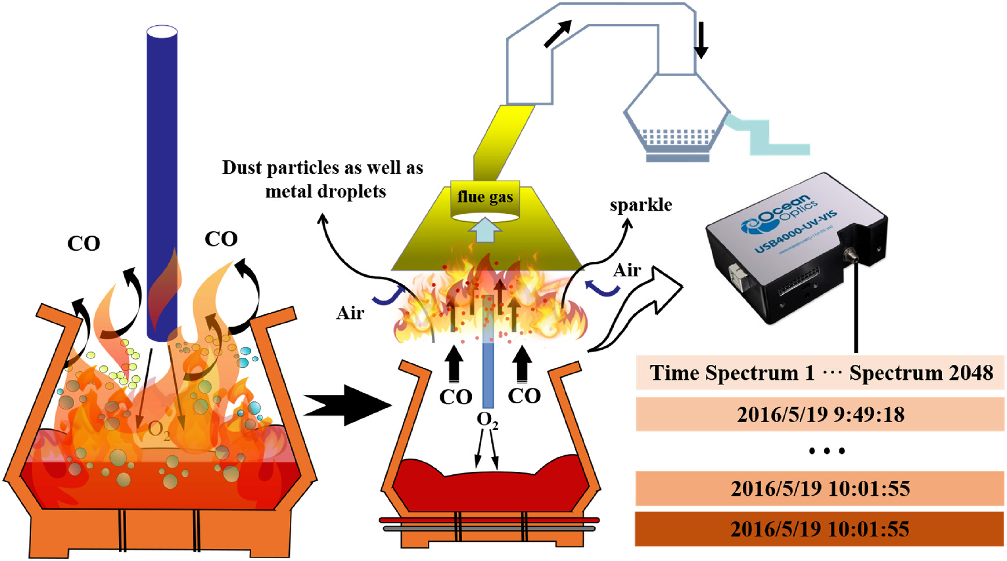
Formation process of blast furnace flame.
Due to the excessively high temperature at the furnace mouth during the steel-making process, there are no effective collection methods available to conduct real-time detection of the CO and CO2 content at the furnace mouth. Therefore, a stainless-steel gas probe is installed in the flue to collect flue gas. After the collected flue gas is cooled and filtered, it is connected to a Raman gas analyzer to detect the changes in the composition of the flue gas inside the furnace. This data is used to characterise the variations in gas composition at the furnace mouth, as shown in Figure 4.
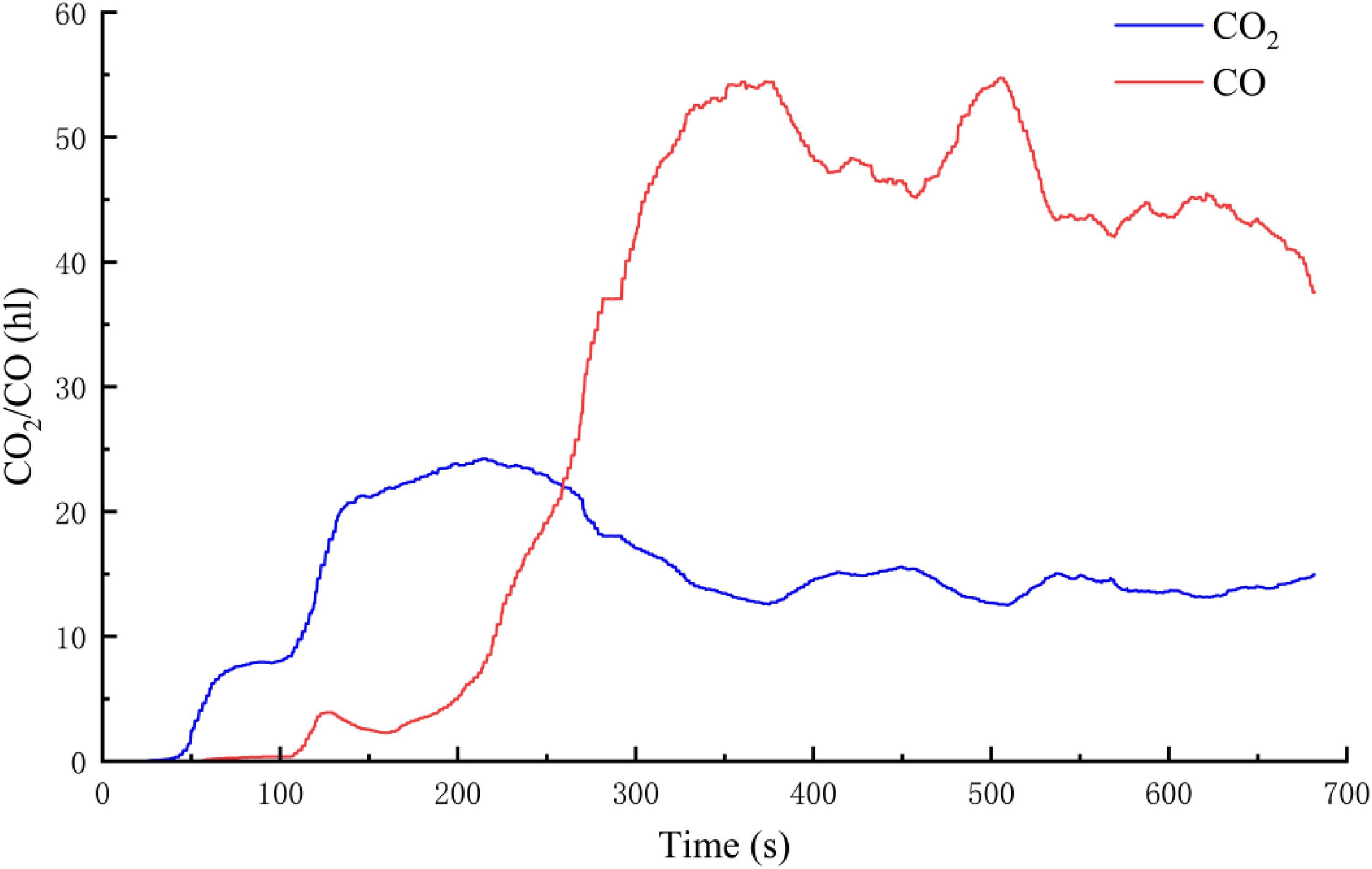
Gas trends of carbon monoxide (CO) and carbon dioxide (CO2).
The production of CO begins to show a noticeable upward trend around 200 s, then fluctuates around 350 s. Then it is relatively stable. In contrast, the production of CO2 largely stabilises after 100 s.
The fitting function of CO and CO2 emissions
Since the emission of CO and CO2 is a continuous process, and the flue gas analysis mass spectrometer employs an intermittent sampling method (sampling interval Δt = 5 s). It is difficult to accurately calculate the total amount of emissions by the direct integration method. To address this, the study proposes a dynamic cumulative modelling method based on function fitting. This approach constructs a continuous emission function to compensate for the information gaps between discrete sampling data points.
To identify the optimal fitting model, this study evaluated five function models: linear polynomial, single exponential polynomial, power-law polynomial, double exponential polynomial and double Gaussian model. The goodness of fit for each model was assessed by comparing the coefficient of determination values calculated after fitting. This comparison was used to determine the optimal function model. Table 2 presents the fitting performance of the different function models for CO emissions.
Five function fitting models for CO fitting R2
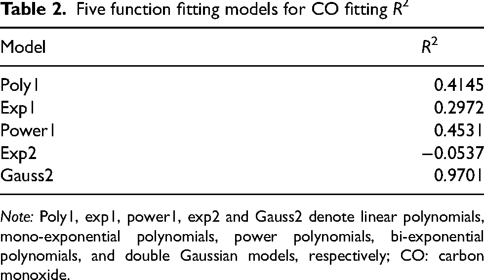
Note: Poly1, exp1, power1, exp2 and Gauss2 denote linear polynomials, mono-exponential polynomials, power polynomials, bi-exponential polynomials, and double Gaussian models, respectively; CO: carbon monoxide.
As shown in Table 2, the double Gaussian model demonstrates the best fitting performance, with an R2 value of 0.9701. This indicates that the model effectively describes the cumulative process of CO emissions and can serve as a reliable foundation for predicting CO emissions in subsequent studies. The functional relationship of the model is as follows:
Figure 5(a) shows the variation curve of CO concentration over time. The measured data (represented by red dots) closely align with the fitted curve (represented by a blue line), demonstrating the accuracy and reliability of the selected fitting model. The change in CO concentration exhibits distinct phase characteristics. In the first 200 s, the CO concentration rises slowly, and then it begins to rise rapidly. Then it reaches a peak of ∼60 mg/m³ between 300 and 400 s. After the peak, the CO concentration shows a fluctuating decline until it drops sharply after 600 s. By integrating the fitted functional relationship of CO, the cumulative emissions are obtained, as shown in Figure 5(b).
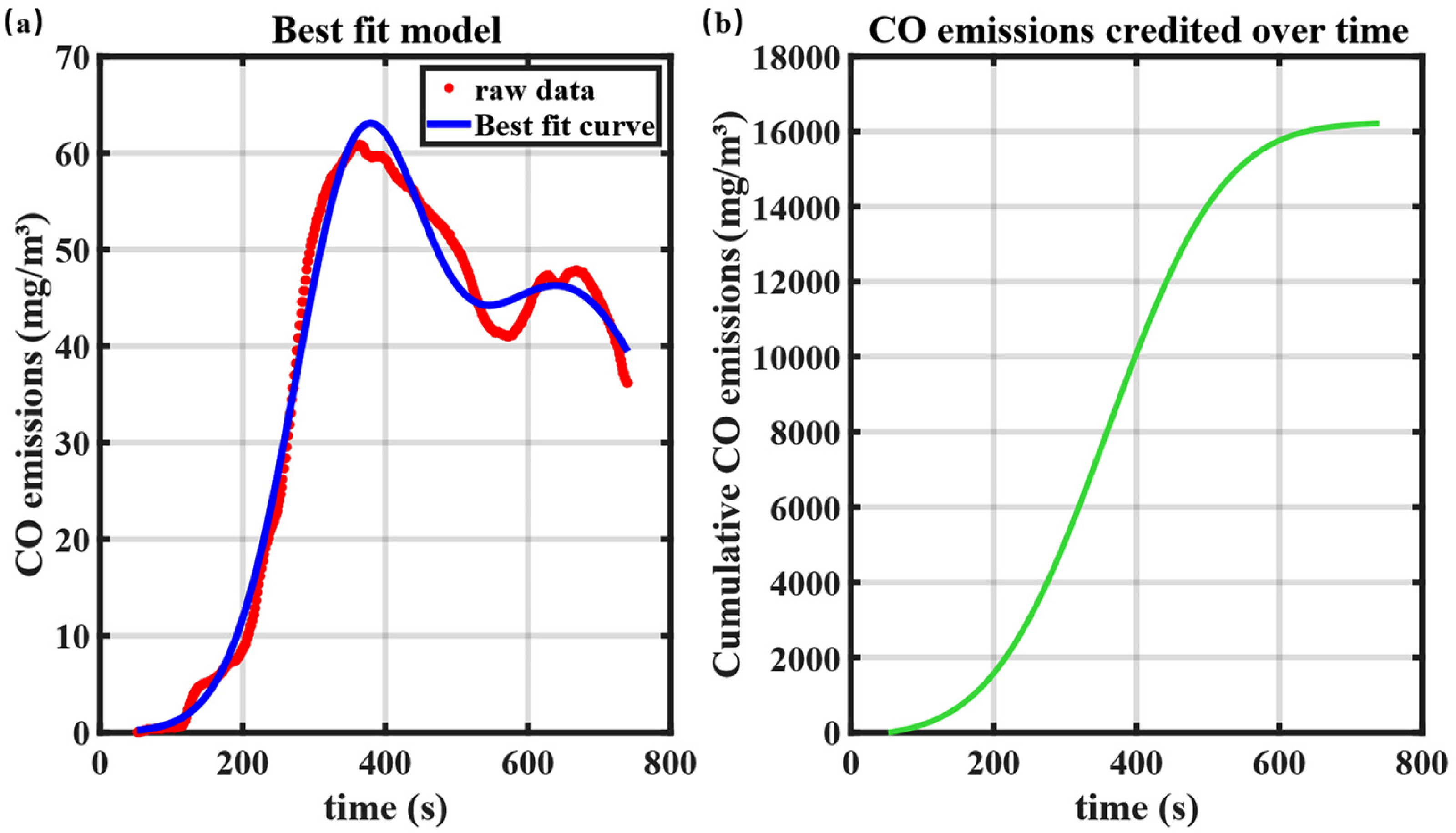
Carbon monoxide (CO) concentration and its fitting curve.
Similarly, the five models are applied to fit CO2 data, with the R2 values presented in Table 3 and the fitting performance is illustrated in Figure 6(a). The double Gaussian model again demonstrates the best fitting performance, achieving an R2 value of 0.9561. The resulting fitted function is as follows. Figure 6(b) displays the cumulative emissions of CO2.
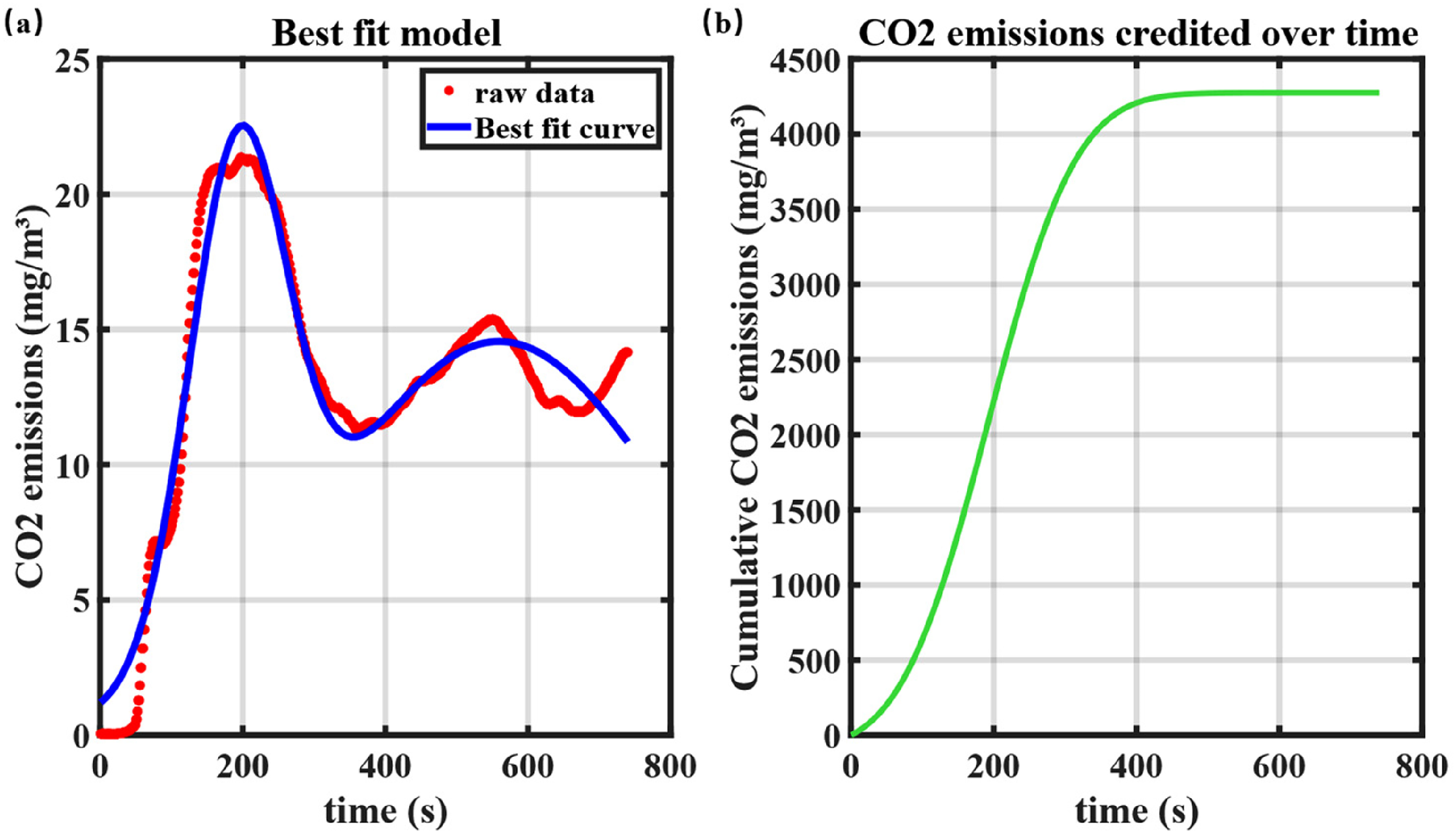
Carbon dioxide (CO2) concentration and its fitting curve.
CO2 fitting R2 of five function fitting models.
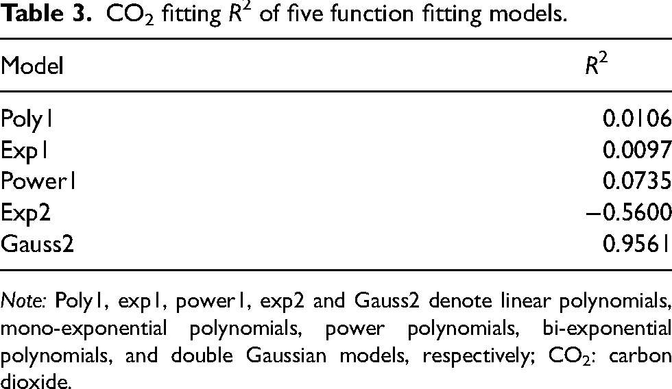
Note: Poly1, exp1, power1, exp2 and Gauss2 denote linear polynomials, mono-exponential polynomials, power polynomials, bi-exponential polynomials, and double Gaussian models, respectively; CO2: carbon dioxide.
Phased changes of spectral characteristics
The cumulative emission curve clearly reflects three distinct phases of the process: an initial phase of slow accumulation, a middle phase of rapid growth, and a final phase of stabilisation, exhibiting a characteristic S-shaped growth trend.
During the converter steel-making process, the emissions of CO and CO2 exhibit stage-by-stage characteristics. By analysing the first-order derivative of cumulative emissions, the inflection points of different emission stages can be accurately determined. And then a reasonable cumulative emission threshold can be determined to divide the stages. The central difference method is used to calculate the first-order derivative of the cumulative emissions. The formula is as follows:
By observing the change trend of the first-order derivative, it is found that when the cumulative emission reaches 5000 mg/m³, the first-order derivative begins to increase significantly, and the CO emission enters a rapid-growth stage. As the carbon content is continuously consumed, the carbon-oxygen reaction rate is gradually limited. When the cumulative emission reaches ∼15,000 mg/m³, the first-order derivative starts to decrease, and the CO emission rate tends to be stable. Similarly, by using 2000 and 4500 as two thresholds, the CO2 emission process is divided into three stages.
For a more intuitive presentation, the segmentation results are visualised in Figure 7. As shown in the figure, the selected thresholds effectively divide the cumulative emissions into distinct stages to provide a foundation for subsequent analysis.
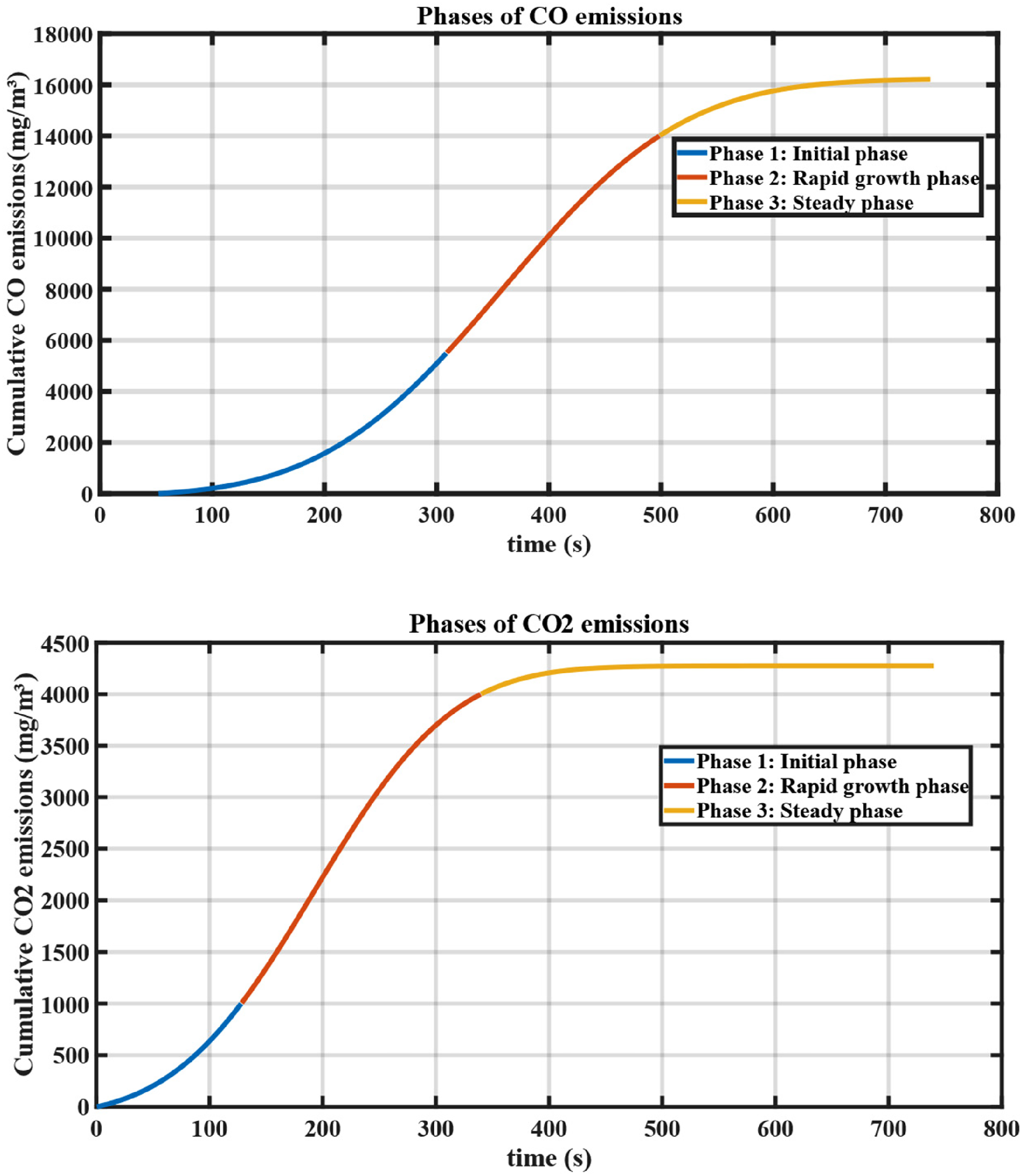
Stage division of carbon monoxide (CO) and carbon dioxide (CO2) emissions.
Dimension reduction analysis of spectral data
The original dimensionality of the spectral data is as high as 2048 dimensions, which imposes a significant computational burden on subsequent model training and prediction, leading to low computational efficiency and potentially reduced prediction accuracy. To improve computational efficiency, reduce model complexity, and retain the key information in the spectral data, it is essential to perform dimensionality reduction. By reducing data dimensionality, this process lowers computational costs while retaining key features, improving both the efficiency of machine learning model training and prediction accuracy.
This study employs a strategy combining an autoencoder and Optuna optimisation for spectral data dimensionality reduction. Optuna, an efficient hyperparameter optimisation tool, employs the Bayesian optimisation algorithm to quickly find the optimal dimension reduction dimension and learning rate through intelligent exploratory search, so as to improve the performance of the model. 26 The dimensionality determines the size of the latent space, while the learning rate influences the speed of network parameter updates and the convergence of the optimisation process.
In order to ensure that Optuna can explore the parameter space fairly and effectively, the autoencoder adopts a unified optimisation algorithm parameter setting for the three stages of CO and CO2. The parameters of the Optuna model are listed in Table 4. The optimisation direction is set to “minimise” to reduce the reconstruction error, ensuring that the data reconstructed by the autoencoder after dimensionality reduction closely approximates the original data.
Optuna model parameters.
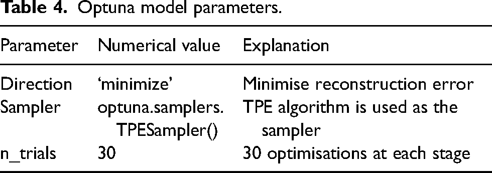
During the optimisation process for each stage, Optuna compares the performance of different parameter combinations to determine the optimal dimensionality and learning rate.
The encoder consists of two fully connected layers. The first layer transforms the dimensionality of the input data to 128 dimensions and employs the ReLU activation function for nonlinear transformation. The second layer maps the 128-dimensional representation to the dimension specified by hyperparameter optimisation, which is the target dimensionality for dimensionality reduction. The decoder mirrors the encoder's architecture but operates in reverse, progressively reconstructing the data from the reduced-dimensional space back to the original input dimensionality. To ensure the effectiveness of the autoencoder, the decoder uses ReLU activation functions in its hidden layers and a sigmoid function in the output layer to constrain the output values within the range [0, 1]. The mean squared error is used as the loss function to quantify the discrepancy between the original data and its reconstruction, guiding the network to learn how to accurately reproduce the input data. The specific best parameters are shown in Table 5.
Optimal parameters of the autoencoder model.
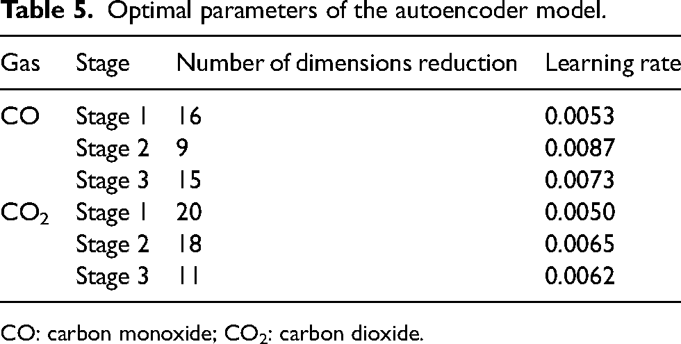
CO: carbon monoxide; CO2: carbon dioxide.
The objective value is the value calculated according to the set objective function for each trial, reflecting the performance of the autoencoder in that trial, such as the reconstruction error. The best value is the optimal value among all the objective values obtained in the current set of trials. As the number of trials increases, the best value drops rapidly and tends to stabilise, indicating that Optuna quickly finds the direction of the optimal hyperparameter combination. At the beginning of the iteration, the objective value fluctuates, and the best value decreases first, and then gradually stabilises after a certain number of trials. This means that the optimisation process gradually converges to a better hyperparameter setting. The iterative optimisation process over multiple trials is illustrated in Figure 8.
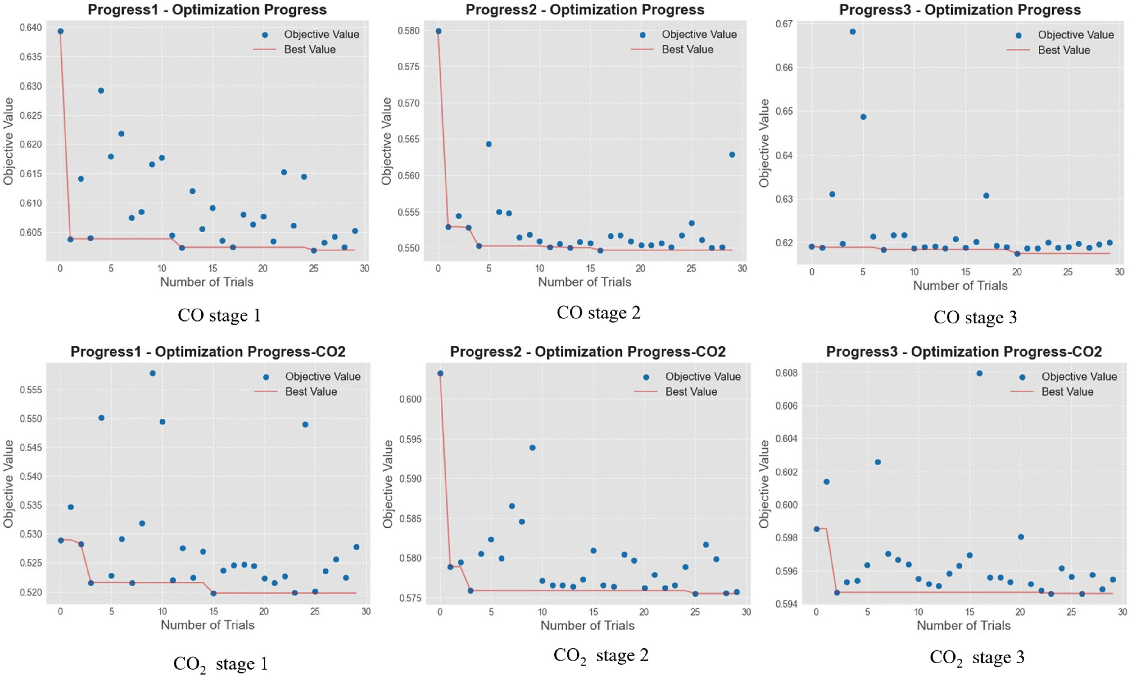
Optuna iteration process.
Analysis of the dimension reduction effect
After completing the dimensionality reduction of the spectral data, this study employs PCA to validate the effectiveness of the reduced data in retaining the information of the original data. The analysis is conducted from three perspectives: reconstruction error (RE), explained variance (EV) and Silhouette score, as detailed in Table 6.
Dimension reduction evaluation results.
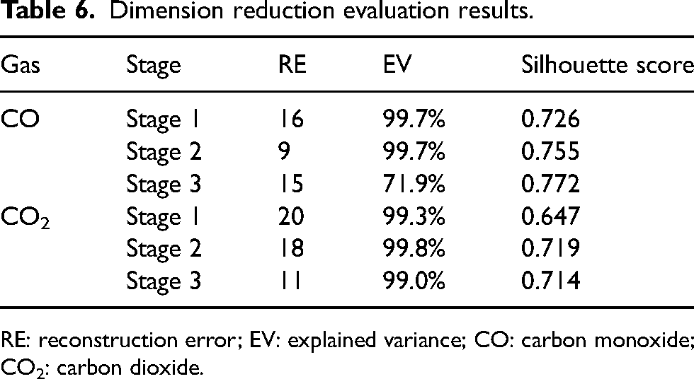
RE: reconstruction error; EV: explained variance; CO: carbon monoxide; CO2: carbon dioxide.
Reconstruction error

Explained variance
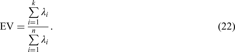
Here,
The explained variance is a commonly used measurement criterion in PCA for dimensionality reduction. It represents the proportion of the total variance that is explained by the first k principal components. The larger the explained variance is, the better the data after dimensionality reduction can retain the features of the original data. When the value of EV is close to 1, it indicates that the information loss after dimensionality reduction is small, and the effect of dimensionality reduction is good.
Silhouette score

Among them, a represents the average distance from a sample point to other points within the same cluster, which indicates the similarity between the sample point and other points in the cluster; b represents the average distance from the sample point to the nearest different cluster, which indicates the similarity between the sample point and other clusters.
The Silhouette score is used to evaluate whether data points are reasonably assigned to different categories in the new space after dimensionality reduction. The value of the Silhouette score ranges from −1 to 1. When S is close to 1, it indicates that the clustering quality of the sample points is good, that is, the similarity between the sample points and other sample points within their cluster is high, and the similarity to other clusters is low. When S is close to 0, it means that the sample points are located at the boundary between two clusters, and the clustering quality is poor. When S is close to −1, it indicates that the sample points may be wrongly assigned to the wrong cluster.
From the dimensionality reduction results of the three stages of CO, it is evident that Stages 1 and 2 achieved significant dimensionality reduction. The variability of most data in these stages can be effectively represented by a few principal components, indicating high linear separability and successful dimensionality reduction. However, the reduction performance in Stage 3 is slightly inferior, with the first two principal components explaining a lower proportion of variance. This suggests that the data in Stage 3 may contain more nonlinear structures or exhibit a more complex distribution, leaving room for improvement in dimensionality compression. Nevertheless, the Silhouette scores for Stages 1–3 are relatively high, at 0.726, 0.755 and 0.772, respectively. This indicates strong clustering effects in these stages, with high intra-class similarity and clear inter-class differences, further confirming the well-defined structure of the data. Additionally, the reconstruction errors across the stages are similar, demonstrating that the dimensionality reduction effectively preserves the original structure and information of the data.
The dimensionality reduction results for the three stages of CO2 reveal that Stage 2 has the highest explained variance, with the first two principal components accounting for 99.8% of the data variance. This indicates a strong linear structure in the principal component space for this stage. The explained variance for Stages 1 and 3 is also high, reaching 99.3% and 99%, respectively, reflecting good linear characteristics. Further analysis shows that the Silhouette scores for Stages 2 and 3 are relatively high, at 0.719 and 0.714, respectively, suggesting effective clustering, strong intra-class similarity, and clear inter-class separation in these stages. In contrast, the clustering effect in Stage 1 is relatively weaker, likely due to lower similarity among data points. The reconstruction errors across the three stages are similar, further demonstrating the autoencoder's effective reconstruction of the data.
To visually demonstrate the dimensionality reduction effect, two-dimensional scatter plots of the data after PCA dimensionality reduction were generated. Figure 9 clearly shows the clustering phenomenon of the reduced data, indicating that the autoencoder successfully extracts key features of the data. Different categories of samples are well-separated in the reduced feature space.
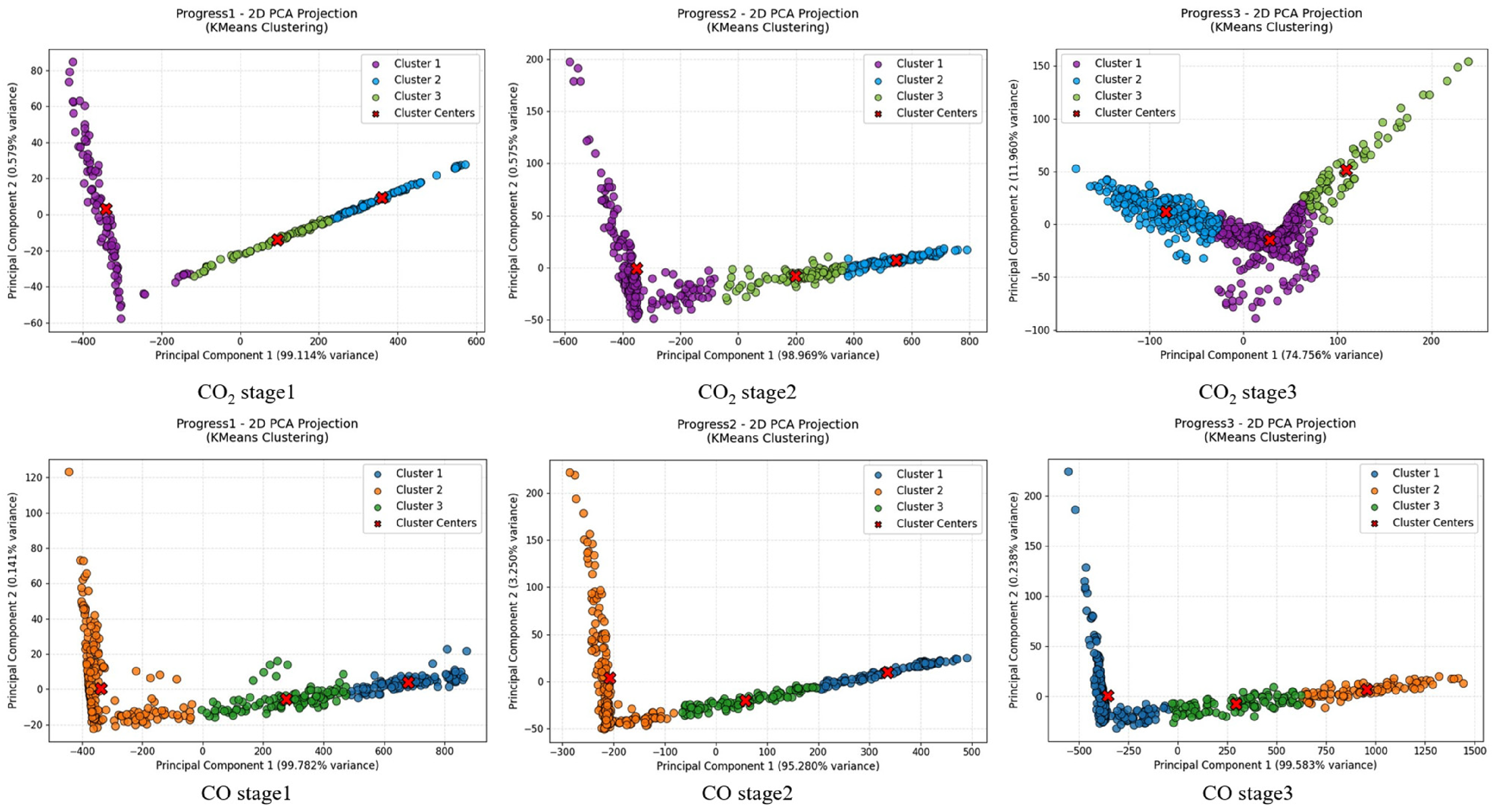
Principal component analysis (PCA) clustering results.
Experimental results and discussion
Parameter optimisation of the GWO algorithm
In this study, the GWO model is employed to optimise the parameters of the BiLSTM prediction model for the three stages of the CO and CO2 fitting curves.
When using the GWO to optimise the BiLSTM network, the number of training epochs is set to 70, the batch size is set to 1/10 of the entire dataset, the population size of the algorithm is set to 10, and the number of algorithm evolutions is set to 20.
In the process of parameter optimisation of the GWO algorithm, the number of hidden layer nodes is set within the range [20, 100], and the discard rate is set as a real number in the interval of [0.01, 0.2]. The determination of these search ranges is based on previous pre-experiments and domain knowledge, which not only ensures sufficient exploration space but also avoids invalid parameter combinations. The optimised hyperparameters include the number of hidden layer nodes and the dropout rate. For example, in the optimised configuration for CO Stage 1, the optimal network architecture features 50 hidden layer nodes with a dropout rate of 0.05729. This configuration effectively captures the drastic changes in carbon content during the initial decarburisation phase. Conversely, in the optimised configuration for CO2 Stage 3, the network architecture becomes more compact, with 45 hidden layer nodes and a dropout rate of 0.0535, reflecting the reaction characteristics when carbon content stabilises in the final stage. By adjusting these hyperparameters, the GWO algorithm ensures that the model can adapt to different phases of the converter steelmaking process, thereby enhancing prediction accuracy.
In the 25 iterations of CO2 Stage 3, the GWO algorithm ensures the precise convergence of the optimisation result. In contrast, only 15 iterations are required in CO Stage 1. Through the fine adjustment during the GWO optimisation process, the model is able to perform appropriate parameter configuration according to the characteristics of each stage.
The optimal parameters of the BiLSTM model obtained are presented in Table 7. The iterative process of the GWO model across six different stages is visualised in Figure 10.
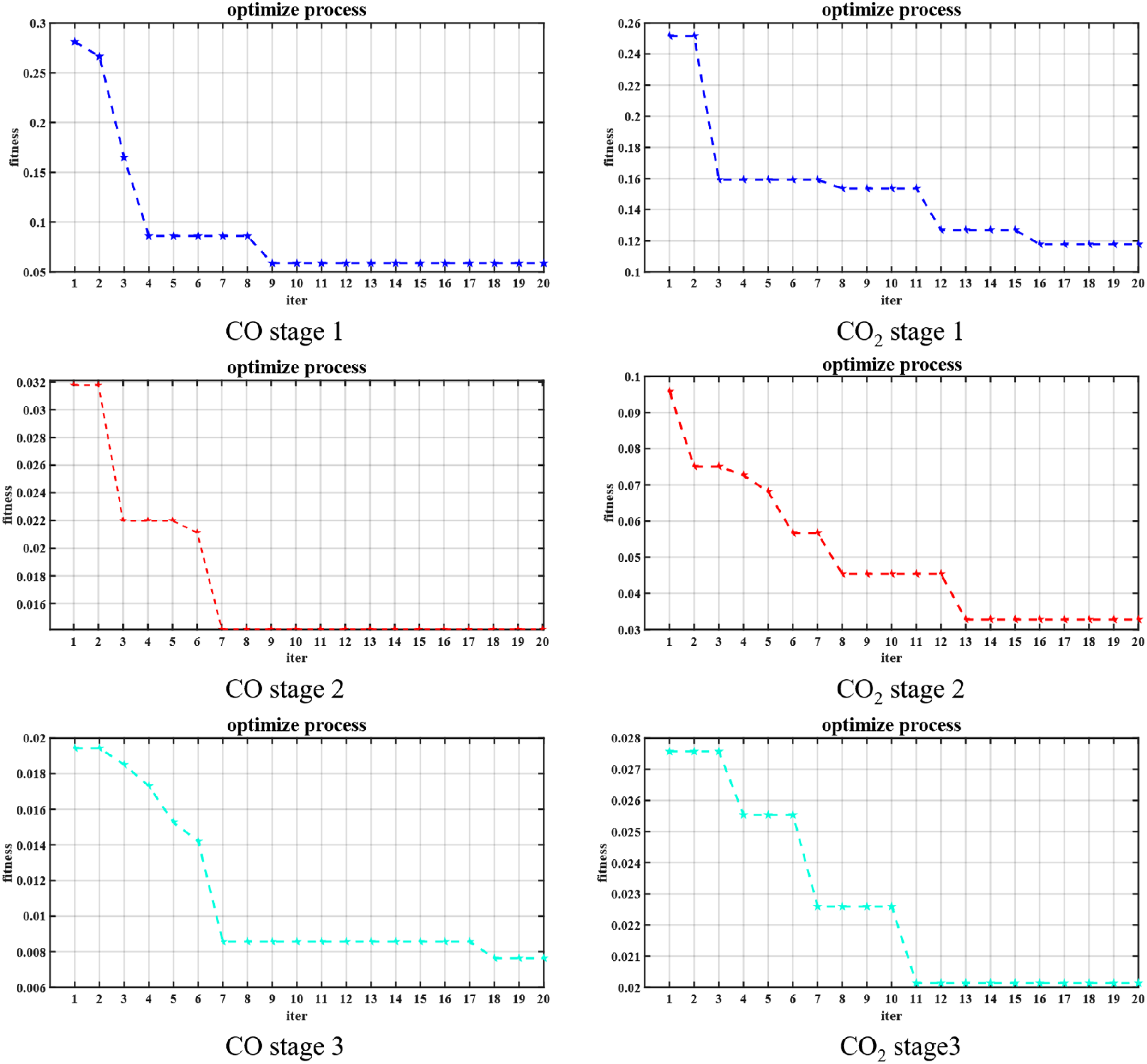
Grey wolf optimisation (GWO) iteration process diagram.
Optimisation results for GWO.

GWO: Grey wolf optimisation; CO: carbon monoxide; CO2: carbon dioxide.
The GWO algorithm shows an obvious convergence trend during the iterative process. As the number of iterations increases, the optimisation objective gradually approaches the optimal solution. The convergence rate remains stable during the adjustment of parameters such as the number of hidden layer nodes and the dropout rate of the BiLSTM model, reflecting the adaptability of the algorithm to the prediction of the carbon content in the steel production process. The iterative curve in the figure does not exhibit obvious stagnation or oscillation phenomena, indicating that the GWO algorithm has a strong ability to explore the parameter space and can effectively avoid falling into local optimal solutions.
The prediction results of BiLSTM
The optimal parameters are input into the BiLSTM model, along with the optimal features obtained from PCA dimensionality reduction of the original data, to predict the variations of CO and CO2 across different stages. The prediction results are compared with the original data, demonstrating that the model exhibits high accuracy and effectively captures the trends in the time-series data. The comparison between the predicted results and the original data is visualised in Figure 11.
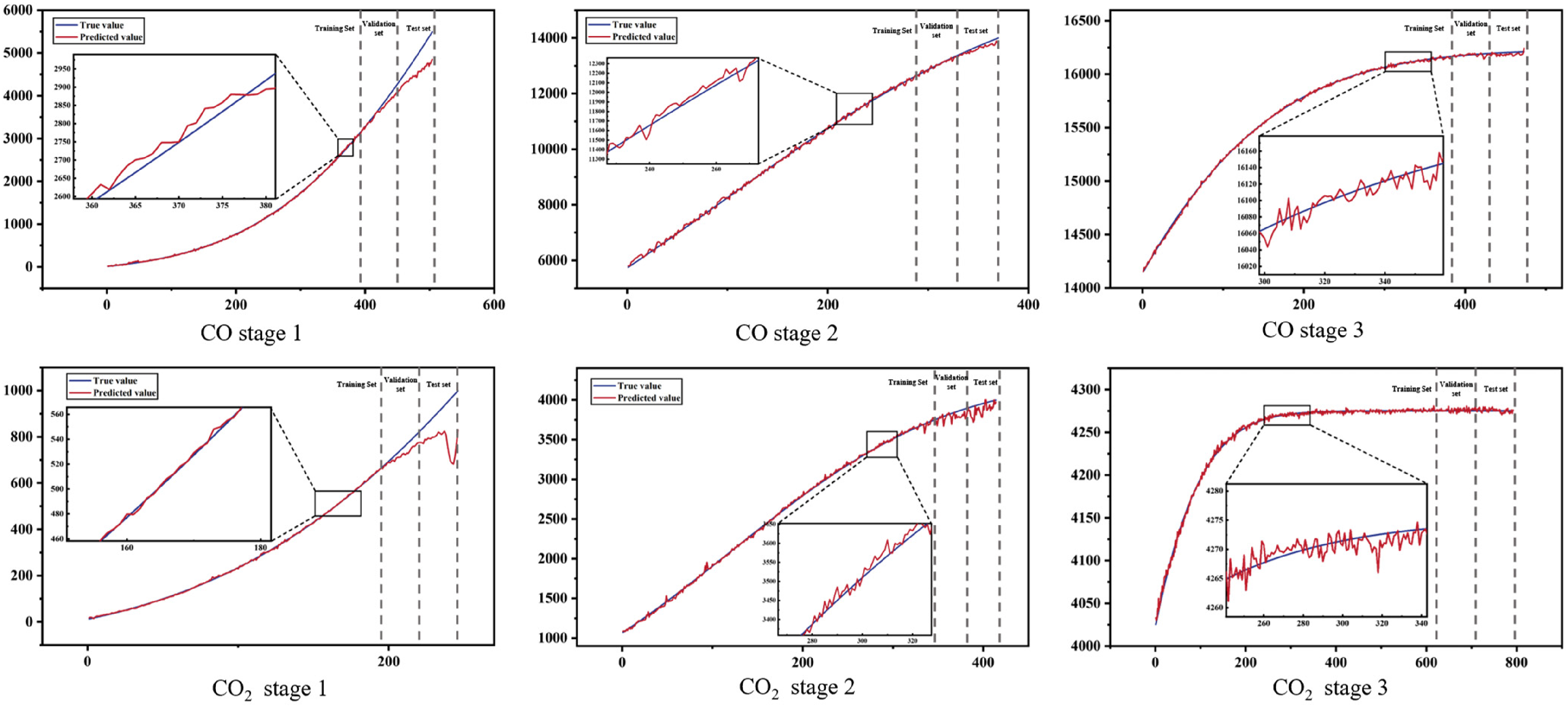
Comparison of prediction results.
Judging from the images of each stage, the predictions of the cumulative emissions of CO and CO2 by the BiLSTM model are relatively close to the true values in terms of trend. For example, in stages such as CO Stage 2 and CO2 Stage 2, the prediction curve can follow the upward trend of the true value curve, indicating that the model can capture the pattern of the changes in the cumulative emissions of CO and CO2 over time to a certain extent, and has the basic ability to fit the trend of gas emissions during the steelmaking process. However, in CO Stage 1, there are some deviations between the predicted values and the true values.
Considering the comprehensive performance across multiple stages, the prediction effects of the model vary across different stages. The working conditions and emission characteristics change in different steelmaking stages, and the BiLSTM model cannot always maintain stable and accurate predictions. Its adaptability is limited when facing changes in working conditions, making it difficult to provide high-precision prediction results throughout the steel-making process.
Experimental comparison
In order to comprehensively and objectively evaluate the performance of the model in predicting the emissions of CO and CO₂ during converter steelmaking, this study selects three indicators, namely MAE, RMSE and MAPE, for a comprehensive evaluation.27–31


Among them,
In the performance evaluation of different models, for the prediction of CO and CO2 emissions in different stages, we compare the GWO-BiLSTM model with the BP, LSTM, BiLSTM and transformer models. The collected data is divided into a training set and a test set at a ratio of 7:3, and the data of both sets are, respectively, input into the above-mentioned models for training. The results of these metrics across the six stages are presented in Table 8.
Model prediction results.
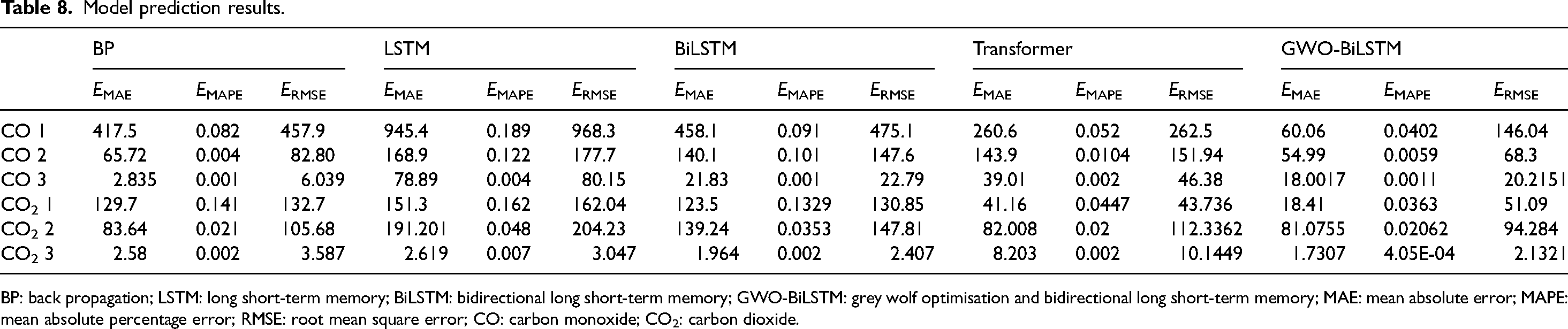
BP: back propagation; LSTM: long short-term memory; BiLSTM: bidirectional long short-term memory; GWO-BiLSTM: grey wolf optimisation and bidirectional long short-term memory; MAE: mean absolute error; MAPE: mean absolute percentage error; RMSE: root mean square error; CO: carbon monoxide; CO2: carbon dioxide.
Based on the results in Table 8, the BiLSTM model exhibits varying levels of accuracy across different stages during the prediction process. For the three stages of CO, the model's performance improves progressively as the stages advance. Specifically, in the first stage of CO, MAE is 60.06, MAPE is 0.0402 and RMSE is 146.04, indicating relatively large prediction errors at this stage. In the second stage of CO, MAE decreases to 54.99, MAPE decreases to 0.0059 and RMSE decreases to 68.3, showing improved prediction accuracy. By the third stage of CO, MAE further drops to 18.0017, MAPE further drops to 0.0011 and RMSE significantly decreases to 20.2151, demonstrating high prediction accuracy and suggesting that the model can effectively capture data trends at this stage.
For the three stages of CO2, the results also show a gradual optimisation trend. In the first stage of CO2, MAE is 18.41, MAPE is 0.0363 and RMSE is 51.09, indicating relatively ideal prediction performance. In the second stage of CO2, although MAE increases to 81.0755, MAPE increases to 0.02062 and RMSE increases to 94.284, the prediction accuracy declines. Finally, in the third stage of CO2, MAE significantly decreases to 1.7307, MAPE decreases to 4.0482 × 10⁻⁴ and RMSE decreases to 2.1321, achieving the best prediction performance, with a notable improvement in model accuracy.
In all stages of CO and CO₂ emissions, MAE values of the GWO-BiLSTM model are relatively low, and MAPE and RMSE values are also the same. This indicates that the GWO-BiLSTM model outperforms the BP, LSTM, BiLSTM and transformer models in terms of prediction accuracy and stability, demonstrating excellent performance and providing a more reliable solution for relevant emission predictions.
Model explainable
SHAP is an interpretable machine learning method used to explain the prediction results of a model, and its principle is based on the Shapley value in cooperative game theory. 32
In order to further illustrate the degree of each feature on the prediction result, waterfall diagrams of different input features are drawn respectively. The left axis represents the feature names and values. Red indicates a positive impact on the prediction result, and blue indicates a negative impact on the prediction result.
As can be seen from Figures 12 and 13, Feature 7 (627.695), Feature 10 (641.605) and Feature 13 (673.682) are the three features that have the greatest influence on the prediction of the converter reaction stage, and their wavelengths are in the range of about 600–750 nm of the oxygen absorption peak during the reaction process. Especially in the CO2 reaction stage (CO2 Stage 2) and the oxygen consumption stage, the fluctuations of these features make a significant contribution to the prediction of the reaction endpoint. In addition, the contributions of Feature 2 (453.29) and Feature 4 (507.959) are relatively low, and their wavelengths are in the range of about 400–500 nm of the nitrogen absorption peak during the reaction process. They have a certain influence in the CO reaction stage (CO Stage 1 and CO Stage 2), but have little influence on the CO2 stage. This analysis of feature importance provides strong evidence for improving the prediction accuracy of the converter reaction endpoint and optimising the relevant process flow.
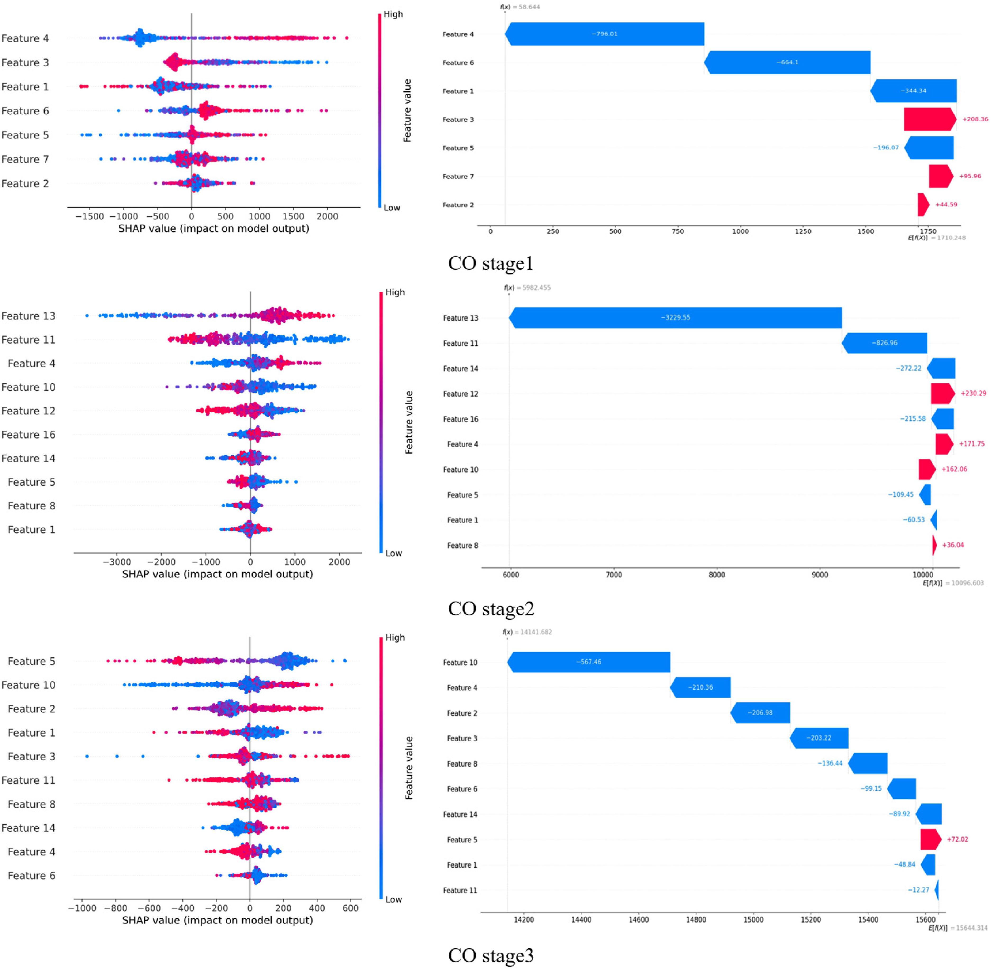
Global interpretability of carbon monoxide (CO).
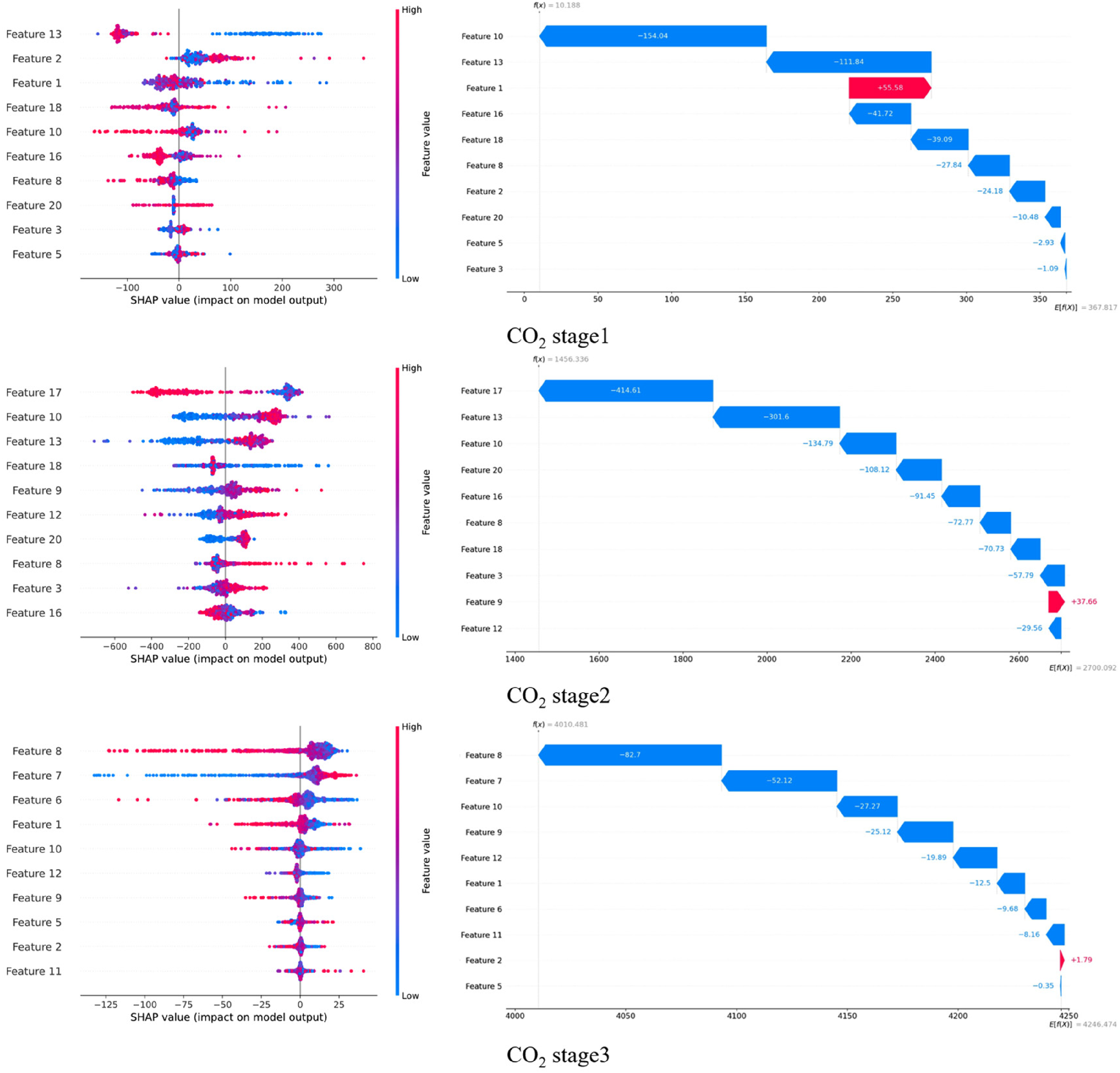
Global interpretability of carbon dioxide (CO2).
Local interpretation
Taking a single sample as an example, in CO stage 1, the cumulative CO emission is 58.64. As shown in Figure 14. Feature 1 (482.5) and Feature 4 (507.959) have a positive effect on the predicted value. Feature 3 (611.3), Feature 5 (619.3), Feature 6 (625.42) and Feature 7 (627.695) have a negative impact on the predicted value.

Local sample explanation.
Conclusions and future work
This article proposes a coal spontaneous combustion temperature prediction model of GWO-BiLSTM, which effectively improves the generalisation ability and robustness of the model, and the following conclusions are drawn:
By combining the autoencoder with the Optuna optimisation method, the 2048-dimensional high-dimensional spectral data is reduced in dimension, which reduces the complexity of the model, improves the computational efficiency, and retains the key information. The GWO is used to optimise the parameters of the BiLSTM prediction model, enabling the model to better capture the trends of time-series data and improving the prediction accuracy. The experimental results show that the GWO-BiLSTM model performs excellently in terms of prediction accuracy and stability. Compared with the BP, LSTM, BiLSTM and transformer models, this model has relatively lower MAE, MAPE and RMSE in all stages of CO and CO2 emission prediction. Especially in the third stage, the prediction errors are significantly reduced. For CO and CO2 gases, MAE decreases to 18.0017 and 1.7307, respectively, and the RMSE decreases to 20.2151 and 2.1321, respectively. Through the model interpretation by the SHAP method, the influence degree of different spectral features on the prediction results is clarified. The features within the wavelength range of 600–750 nm significantly contribute to the prediction of the reaction endpoint in the CO2 reaction stage and the oxygen consumption stage, providing a theoretical basis for optimising the process flow.
Although this study has made significant progress in predicting the carbon content during converter steelmaking, there are still some limitations. In this study, the flue gas data have hysteresis due to the sampling interval and transmission delay, which affects the timeliness of the model's response to the dynamic changes in the steelmaking process and the prediction accuracy. The double Gaussian model fits the emissions of CO and CO2 relatively well, but there are errors in the rapidly changing stages, which affect the calculation of the cumulative amount.
In future research, other optimisation algorithms and model structures can be further explored. By combining more data information in the steelmaking process, such as the composition of the slag and the temperature change, the prediction accuracy and the generalisation ability of the model can be further improved to better meet the actual needs of steel production.
Footnotes
Declaration of conflicting interests
The authors declared no potential conflicts of interest with respect to the research, authorship, and/or publication of this article.
Funding
The authors disclosed receipt of the following financial support for the research, authorship, and/or publication of this article: This work was supported by the Research on Intelligent Research Mechanism of Blast Furnace Condition by Integrating Big Data Deep Learning, Research on Dynamic Correction Model for Flue Gas Analysis Based on Flame Spectral Modulation of Converter Mouth, Research on Intelligent Control Model of Furnace Temperature Based on Deep Mining of Big Data of Blast Furnace Smelting Process (grant numbers 22130201G, QN2023153 and 52074126).
