Identification of continuous casting round blooms shrinkage defects based on deep learning

Abstract

In the continuous casting process, issues such as time lag in macroscopic inspection results and human interference factors hinder efficient quality assessment. Rapid and accurate identification of round bloom quality defects is critical for stabilising production. The study employs a U-Net neural network to preprocess image data from the continuous casting process, achieving a segmentation accuracy of 94.4% for round blooms. Metrics including precision, confusion matrix and ROC curve are used to evaluate the reliability and stability of different mathematical models in predicting defects. The convolutional neural network demonstrates superior performance with a defect identification accuracy of 97.12%, providing actionable guidance for on-site production optimisation.

Keywords

Defects in continuous casting round blooms macroscopic inspection deep learning image recognition continuous casting process

Introduction

Macroscopic inspection of continuous casting blooms is a key technique for evaluating internal quality in steel production.¹ This method analyses macrostructural features of round bloom cross-sections using macroscopic images.^2,3 However, manual inspection suffers from inefficiency and delayed feedback,^4,5 limiting real-time anomaly detection. Thus, developing high-precision defect identification models is essential.

Currently, deep learning image recognition technology is widely applied in medical diagnostics,⁶ agricultural and biological applications,⁷ facial recognition⁸ and other domains. In metallurgy, artificial neural network algorithms have been employed for predicting thermal deformation stress in high-Mn steels,⁹ chemical composition of ferritic stainless steels¹⁰ and high-temperature deformation behaviour of steels.¹¹ Significant research efforts have also been conducted on quality defect identification in continuously cast blooms. Models including LSTM-FCN,¹² XGBoost¹³ and random forests¹⁴ have been employed to predict quality defects based on process equipment data records. However, such data-driven approaches lack direct visualisation capability for defect manifestation. Macroscopic imaging analysis provides intuitive defect characterisation, with algorithms like YOLOv5,¹⁵ VGG,¹⁶ CNN¹⁷ and YOLOv8¹⁸ being implemented for quality defect recognition in low-magnification billet images. However, the approach inadequately addresses the influence of surrounding environmental factors on the continuous casting round blooms. Moreover, shrinkage defect identification remains confined to specific regions, resulting in low applicability for actual production conditions and hampering practical implementation for continuous casting process optimisation. To address the challenge of accurate quality defect identification in industrial environments, an integrated prediction model based on multi-model fusion has been developed.

To address these limitations, the study proposes an integrated multi-model framework. The methodology involves labelling macroscopic images of round blooms using Labelme, followed by U-Net-based segmentation. The model's performance is validated via intersection-over-union (IoU), Dice coefficient, and Hausdorff distance (HD). Preprocessed images are then fed into support vector machine (SVM), naive Bayes (NB) and convolutional neural network (CNN) models for defect classification. Evaluation metrics such as precision, recall, confusion matrix, ROC curve and Matthews correlation coefficient (MCC) are utilised to select the optimal model.

Model architecture design and description

Model architecture design

To address the challenges of environmental interference and time lag in macroscopic inspection of round blooms during continuous casting, this study proposes an integrated deep learning framework for real-time defect identification. As illustrated in Figure 1, the workflow begins with acquiring macroscopic images of round blooms during the continuous casting process. These images are annotated using the Python-based Labelme tool and binarised to serve as the ground truth output for the U-Net segmentation model. The raw images are fed into U-Net as inputs, and segmentation accuracy is rigorously evaluated using metrics such as IoU, Dice coefficient and HD. This preprocessing step effectively isolates the round bloom from background noise, eliminating environmental interference. The segmented images are then fed into a CNN for defect classification, where the output indicates the presence or absence of defects. Classification performance is validated using precision, recall, confusion matrix, ROC curves and MCC to ensure model robustness and stability.

Figure 1.

Framework diagram of integrated recognition model.

U-Net model

U-Net is a mathematical model based on data augmentation in network architecture and training strategies, enabling effective utilisation of limited annotated samples.^19,20 The network architecture consists of a symmetric encoder-decoder structure with skip connections.²¹ The encoder comprises multiple convolutional and downsampling layers, progressively extracting high-level semantic features of the image while reducing the spatial dimensions of the feature maps. The decoder gradually restores the spatial resolution of the feature maps through upsampling, mapping low-resolution high-semantic features back to the original image size. Each upsampling layer is connected to the corresponding encoder layer via skip connections. These skip connections directly concatenate the feature maps from each encoder layer to the corresponding decoder layer, addressing the loss of spatial information caused by downsampling, achieving multi-scale feature fusion, and enhancing segmentation localisation capability.^22,23

U-Net is an end-to-end training model.²⁴ As shown in Figure 2, the raw image is input and processed through 3 × 3 convolutions with ReLU activation functions. Local features of the image are gradually extracted via connections to max-pooling layers. The image is then reconstructed through upsampling, skip connections and convolutional operations to achieve segmentation prediction.

Figure 2.

Operational principle of U-Net in eliminating peripheral artefacts from low-power imaging through computational segmentation.

The evaluation of image segmentation models primarily focuses on boundary accuracy, and volumetric similarity.²⁵ Metrics such as IoU,²⁶ Dice coefficient²⁷ and HD²⁸ are selected to evaluate the accuracy and reliability of the U-Net model.

IoU = \frac{| A \cap B |}{| A \cup B |}

(1)

Dice = \frac{2 | A \cap B |}{| A | + | B |}

(2)

The HD is used to quantify the maximum mismatch between two sets of points. For two point sets $C = {a_{1}, a_{2}, \dots a_{m}} and D = {b_{1}, b_{2}, \dots b_{n}}$ , Hausdorff distance $H = (C, D)$ is defined as:

H (C, D) = \max (h (C, D), h (D, C))

(3)

where

h (C, D)

represents the directed Hausdorff distance from set C to set D, defined as the maximum of the minimum distances between points in C and D:

h (C, D) =_{a \in C}^{\sup} (_{b \in D}^{\inf} d (a, b))

(4)

where

d (a, b)

denotes the Euclidean distance between points c and d, sup represents the maximum value in the set, inf represents the minimum value in the set.

CNN model

The CNN²⁹ is a mathematical model specifically designed for processing grid-like data. Its image processing workflow is illustrated in Figure 3. The structure consists of two main components: a feature extraction section and a classification section.³⁰ The feature extraction section performs a series of convolutional and pooling operations.³¹ The classification section uses fully connected layers as a classifier, assigning probabilities to objects in the image based on features extracted by the feature extraction section and outputting image labels.³²

Figure 3.

Feature parameter extraction of continuous casting round blooms low-magnification images using convolutional neural networks.

The detailed architecture of the CNN is illustrated in Figure 4, comprising sequentially stacked convolutional layers with ReLU activation, spatial downsampling through max-pooling operations and fully connected layers for classification. Batch normalisation is applied after each convolutional stage to enhance training stability.

Figure 4.

Detailed computational architecture of the CNN.

Metrics including precision, recall, confusion matrix, ROC curves and MCC are chosen to evaluate the reliability and stability of the multi-model fusion approach.^33,34

P r e c i s i o n = \frac{T P}{T P + F P}

(5)

R e c a l l = \frac{T P}{T P + F N}

(6)

C o n f u s i o n m a t r i x = [\begin{matrix} T N & F P \\ F N & T P \end{matrix}]

(7)

R O C = {\begin{matrix} T P R = \frac{T P}{T P + F N} \\ F P R = \frac{F P}{F P + T N} \end{matrix}

(8)

M C C = \frac{T P \times T N - F P \times F N}{\sqrt{(T P + F P) (T P + F N) (T N + F P) (T N + F N)}}

(9)

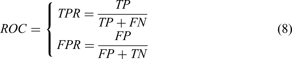
In equations (5) to (9), TP represents the number of samples correctly predicted as positive by the model, FP denotes the number of samples incorrectly predicted as positive, FN indicates the number of samples incorrectly predicted as negative, and TN signifies the number of samples that are truly negative and predicted as negative. These evaluation metrics are core tools for assessing classification models, comprehensively measuring model performance from diverse perspectives.

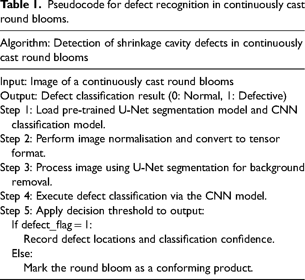
To validate model feasibility, verification was conducted using data not employed in model training, with specific steps detailed in Table 1.

Table 1.

Pseudocode for defect recognition in continuously cast round blooms.

Algorithm: Detection of shrinkage cavity defects in continuously cast round blooms
Input: Image of a continuously cast round blooms
Output: Defect classification result (0: Normal, 1: Defective)
Step 1: Load pre-trained U-Net segmentation model and CNN classification model.
Step 2: Perform image normalisation and convert to tensor format.
Step 3: Process image using U-Net segmentation for background removal.
Step 4: Execute defect classification via the CNN model.
Step 5: Apply decision threshold to output:
If defect_flag = 1:
Record defect locations and classification confidence.
Else:
Mark the round bloom as a conforming product.

Computational results and evaluation of U-Net model

A total of 240 macrographic examination images of continuous casting round blooms, each measuring 1280 × 1280 pixels, were collected from the production site. Images depicting round blooms with and without shrinkage porosity were organised and distributed into training and testing sets. The data partition is detailed in Table 2.

Table 2.

Data distribution and partition.

Data characteristic	Training set	Test set
Images with shrinkage porosity	30	8
Images without shrinkage porosity	162	40

The model was built on the PyTorch framework. To process large-scale image data, a distributed training cluster comprising 6 NVIDIA GeForce RTX 4070 GPUs was implemented, with the system equipped with 256GB of DDR5 RAM. Macroscopic inspection images of round blooms from the continuous casting production site were collected and used for training and simulation with the U-Net model. As shown in Figure 5, the original images were annotated to generate binarised images. The U-Net model predicted the binarised images, with edge errors observed in the predicted results. After post-processing, the restored round bloom images were compared between defective and non-defective cases, demonstrating the model's capability to accurately eliminate environmental interference. The QR-code corresponds to process data in the continuous casting process and does not affect shrinkage defect identification.

Figure 5.

Binarisation processing and U-Net model prediction and reconstruction of continuous casting round blooms low-magnification images.

The accuracy of the U-Net model was validated using IoU and Dice coefficient. As illustrated in Figure 6, the peak precision values for IoU and Dice coefficient are 0.942 and 0.965, respectively, with precision intervals of [0.894, 0.992] and [0.913, 0.998]. These results confirm the model's strong performance in predicting round bloom images.

Figure 6.

Computation of intersection over union and Dice coefficient.

HD, which measures the maximum mismatch between predicted and ground truth boundaries and is sensitive to segmentation edges, was employed for evaluation. Figure 7 shows high overlap between ground truth and predicted boundaries, verifying the reliability of the U-Net model in identifying round blooms.

Figure 7.

Simulation of Hausdorff distance (HD) calculation.

To assess the model's stability, the mean values and variances of IoU, Dice coefficient and HD were calculated for the test dataset. As presented in Table 3, the IoU and Dice coefficient achieve high precision values of 0.944 and 0.971, respectively, with low variances. Although the HD exhibits a high mean value, its overall variance remains low, proving the model's suitability for predicting continuous casting round blooms.

Table 3.

Mean values and variances of evaluation metrics.

Evaluation metrics	Mean	Variance	Performance specifications
IoU	0.944	0.0281	Segmentation overlap accuracy: 94.4%
Dice coefficient	0.971	0.0185	Volume similarity: 97.1%
HD	5.12	0.94	Boundary matching error: < 6 pixels

Computational results and evaluation of CNN model

SVM, NB and CNN were applied to identify round bloom quality defects. Their performance was evaluated using precision, recall and MCC. As presented in Table 4, the CNN model achieved higher prediction accuracy compared to SVM and NB, with precision differentials of 2.54% and 1.67% respectively. For more intuitive comparison of model precision, Figure 8 illustrates through radar chart that the CNN model performed favourably across all evaluation metrics, attaining 97.15% precision. This demonstrates its applicability for predicting shrinkage cavity defects in continuously cast round blooms.

Figure 8.

Radar chart comparing prediction accuracy across models.

Table 4.

Model accuracy comparison.

Evaluation index	SVM	Naive Bayes	CNN
Precision/%	94.58	95.45	97.12
Recall/%	94.92	95.68	97.45
MCC/%	72.68	73.35	81.25

The confusion matrix visually compares prediction results with ground truth labels. In Figure 9, the CNN algorithm demonstrates optimal performance, with only one false negative (FN) and one false positive (FP), confirming its applicability for predicting round bloom defects during continuous casting.

Figure 9.

Confusion matrices for defect classification performance evaluation.

ROC curves reflect the trade-off in model performance under different classification thresholds. As depicted in Figure 10, the area under the curve (AUC) ranges between [0, 1], with higher values indicating superior overall performance. The CNN model achieves the highest AUC of 0.98, further validating its excellence.

Figure 10.

ROC curves and corresponding AUC values.

Model efficiency was evaluated using training time and testing time. As shown in Table 5, CNN exhibited longer computational times compared to SVM and NB, but achieved higher accuracy. To verify model independence, tests were conducted using images excluded from model training. The computational time from initial image input to final defect recognition in round blooms was under 9 s, meeting on-site detection requirements.

Table 5.

Comparison of model efficiency.

Evaluation index	SVM	Naive Bayes	CNN
Train times/min	15	13	18
Test times/min	5	4	6
Per-image inference time/s	8	7	9

Model accuracy and effectiveness were analysed using precision, recall, confusion matrix, ROC curve and MCC. Model efficiency was evaluated via per-image inference time. The CNN algorithm achieved a prediction accuracy of 97.12% with a defect recognition time of 9 s per image, demonstrating applicability for identifying shrinkage cavity defects in continuously cast round blooms.

Conclusions

Macroscopic inspection images of round blooms in continuous casting production are systematically organised. Image segmentation and feature enhancement are performed using a U-Net neural network, followed by defect feature extraction and classification through the CNN applied to preprocessed images. The methodology significantly enhances quality control capabilities in continuous casting production lines through automated defect detection.

The accuracy and reliability of the U-Net model are rigorously validated using three metrics: IoU, Dice coefficient and HD. The model achieved precision values of 0.944 for IoU, 0.971 for Dice coefficient and 5.12 mm for HD, with a variance (σ²) below 0.015 across all measurements. These results confirmed the model's stability and generalisation capability for industrial applications in continuous casting bloom prediction.

Comprehensive evaluation of three classification algorithms SVM, NB and CNN are conducted using precision, recall, confusion matrices, ROC curves and MCC. The CNN algorithm demonstrates superior performance in defect identification, achieving precision, recall and MCC values exceeding 97.15%, with 12.7% and 18.4% improvements over SVM and NB algorithms respectively. Classification superiority is further verified through confusion matrix visualisation and quantitative assessment of ROC curve analysis.

The integrated model is suitable for identifying shrinkage cavity defects in continuously cast round blooms. To extend applicability to different billet types, retraining of the U-Net model accounting for environmental factors is required. Beyond shrinkage cavities, additional defects including cracks and segregation necessitate supplementary data to enhance model universality.

Footnotes

Declaration of conflicting interests

The authors declared no potential conflicts of interest with respect to the research, authorship, and/or publication of this article.

Funding

The authors disclosed receipt of the following financial support for the research, authorship, and/or publication of this article: The present work was financially supported by the National Natural Science Foundation of China (Nos. 52074207 and 52304358) and Young Elite Scientists Sponsorship Program by CAST (No. YESS20230462).

ORCID iD

Xiaoming Li

References

Liu

Wang

Sun

, et al. Research on a new detection method of slab surface crack in mould during continuous casting. Metall Etall Res Techol 2018; 115: 82.

Zhao

Ouyang

Chen

, et al. Surface defects inspection method in hot slab continuous casting process. Ironmak Steelmak 2011; 38: 464–470.

Konovalenko

Marushchak

Kuz

. A method for processing and analysis of the images of a network of thermal fatigue cracks on the surfaces of rollers of continuous casting machines. Mater Sci 2018; 54: 175–183.

Meng

Luo

Wang

, et al. A detection model for corner cracks of continuous casting strand based on deep learning. Ironmak Steelmak 2022; 49: 1048–1056.

Wang

Cheng

, et al. Investigation on mold breakout prediction methods based on image recognition via convolutional neural network. Metall Mater Trans B 2024; 55: 2685–2698.

Zhang

Qiao

. An evolutionary deep learning method based on improved heap-based optimization for medical image classification and diagnosis. IEEE Acces 2024; 12: 102745–102773.

Zhu

Liu

, et al. Deep learning for smart agriculture: concepts, tools, applications, and opportunities. Int J Agric Biol Eng 2018; 11: 13.

Zheng

, et al. Facial expression recognition based on YOLOv8 deep learning in complex scenes. Int J Inf Commun Technol 2025; 26: 89–101.

Churyumov

Kazakova

. Prediction of true stress at hot deformation of high manganese steel by artificial neural network modeling. Materials 2023; 16: 1083.

10.

Honysz

Soria, Beatriz

, et al. Modeling the chemical composition of ferritic stainless steels with the use of artificial neural networks. Metals 2021; 11: 724.

11.

Churyumov

Kazakova

Churyumova

. Modelling of the steel high-temperature deformation behaviour using artificial neural network. Metals 2022; 12: 447.

12.

Geng

Wang

, et al. A deep learning framework for predicting slab transverse crack using multivariate LSTM-FCN in continuous casting. ESWA 2025; 260: 125413.

13.

Wang

Zhou

, et al. Prediction and feature analysis of entrapped slag defect on casting slab based on optimized XGBoost model. Metall Mater Trans B 2024; 55: 2026–2036.

14.

Guo

. Real-time quality prediction of casting billet based on random forest algorithm. IEEE Acces 2018: 140–143.

15.

Yang

Fang

Liu

, et al. Improved YOLOv5 based on feature fusion and attention mechanism and its application in continuous casting slab detection. IEEE TIM 2023; 72: 1–16.

16.

Lian

Sun

Liu

, et al. Automatic recognition and intelligent analysis of central shrinkage defects of continuous casting billets based on deep learning. J Iron Steel Res Int 2023; 30: 937–948.

17.

Lin

Yao

, et al. Detection of a casting defect tracked by deep convolution neural network. Int J Adv Manuf Tech 2018; 97: 573–581.

18.

Fang

Yang

, et al. Improved lightweight YOLOv8 with DSConv and reparameterization for continuous casting slab detection on embedded device. IEEE TIM 2025; 74: 3509532.

19.

Beeche

Singh

Leader

, et al. Super U-Net: a modularized generalizable architecture. PR 2022; 128: 108669.

20.

Gong

Yang

Gan

, et al. Fully automated construction of a deep U-net network model for medical image segmentation. Sensor Mater 2023; 35: 4633–4652.

21.

Senapati

Basu

Deb

, et al. Sharp dense U-Net: an enhanced dense U-Net architecture for nucleus segmentation. IJMLC 2024; 15: 2079–2094.

22.

Yin

Shao

. CFU-Net: a coarse–fine U-Net with multilevel attention for medical image segmentation. IEEE TIM 2023; 72: 1–12.

23.

Han

Zhou

Xie

, et al. Multi-level U-net network for image super-resolution reconstruction. Displays 2022; 73: 102192.

24.

Rajamani

Rani

Siebert

, et al. Attention-augmented U-Net (AA-U-Net) for semantic segmentation. SIVP 2023; 17: 981–989.

25.

Peng

Varshney

. On performance limits of image segmentation algorithms. CVIU 2015; 132: 24–38.

26.

, et al. Distribution-Aware margin calibration for semantic segmentation in images. IJCV 2022; 130: 95–110.

27.

Wang

Pan

, et al. Resformer-Unet: a U-shaped framework combining ResNet and transformer for segmentation of strip steel surface defects. ISIJ Int 2024; 64: 67–75.

28.

Zhang

Han

, et al. An efficient approach to directly compute the exact Hausdorff distance for 3D point sets. Integr Comput-aid E 2017; 24: 261–277.

29.

Elanangai

Vasanth

. An automated steel plates fault diagnosis system using adaptive faster region convolutional neural network. JIFS 2022; 43: 7067–7079.

30.

Zeng

Wang

Chen

, et al. Surface defect identification method for hot-rolled steel plates based on random data balancing and lightweight convolutional neural network. Signal Image Video P 2024; 18: 5775–5786.

31.

Huang

Dai

Sun

, et al. Recognition of converter steelmaking state based on convolutional recurrent neural networks. Metall Mater Trans B 2024; 55: 1856–1868.

32.

Zhou

. Defect detection of hot rolled steels with a new object detection framework called classification priority network. CIE 2019; 128: 290–297.

33.

Lis

. An Analysis of the effect of skew rolling parameters on the surface quality of C60 steel parts using classification models. Materials 2024; 17: 5362.

34.

Wang

Ding

Shahrampour

. TAKDE: temporal adaptive kernel density estimator for real-time dynamic density estimation. IEE IPAMI 2023; 45: 13831–13843.