Interpretable machine learning for high-precision wall thickness prediction of hot-rolled seamless steel tubes

Abstract

To improve the accuracy of axial wall thickness prediction and reduce reliance on manual measurements in hot-rolled steel tube production, a prediction method based on particle swarm optimisation (PSO) and a one-dimensional convolutional neural network (1D-CNN) was developed. A dataset was constructed from 131 industrial samples collected from the production line. An input variable set was established to characterise entry wall thickness, geometric and overall deformation indicators, pass schedule profile features, speed schedule profile and thermal conditions. PSO was then employed to optimise the key hyperparameters of the 1D-CNN. The proposed model was compared with several machine learning models. The results showed that the PSO-1D-CNN model achieved the best predictive performance, with a test root mean square error of 0.0281, a mean absolute error of 0.0217, and a coefficient of determination R² of 0.913. Further interpretability analysis using SHapley Additive exPlanations revealed that the centroid of the reduction distribution, the number of stands, the diameter-to-wall ratio, the tube temperature at the sizing exit, and the radial compression ratio were the most influential variables affecting the predictions. Finally, the proposed model was integrated into an online system. This system enables single tube wall thickness prediction, sawing parameter calculation, and batch visualisation for process adjustment and sawing decisions.

Keywords

Seamless steel tube machine learning wall thickness prediction hot rolling interpretability analysis

Introduction

Hot-rolled seamless steel tubes are critical materials in energy and advanced equipment manufacturing, where dimensional accuracy directly affects structural safety and production costs.¹ In hot rolling, sizing is the final stage for determining the finished diameter and wall thickness, and its deformation depends on the coordinated action of radial compression and axial tension across multiple stands. However, unstable inter-stand tension at the tube ends often causes non-uniform deformation and end thickening, leading to conservative trimming and excessive removal of qualified material. In addition, wall thickness profiles with high spatial resolution are mainly acquired through laborious manual measurements, which severely restricts sample availability and poses a typical small-sample challenge in industrial modelling.² Therefore, developing an accurate prediction model under limited industrial samples remains an urgent challenge.

With the development of industrial big data and machine learning (ML) technologies, data-driven methods have been increasingly applied to capture nonlinear relationships that are difficult to describe through analytical methods.³ Earlier studies have shown that artificial neural networks (ANNs) can be effectively used for complex nonlinear physical estimation tasks when direct analytical modelling or dense sensor measurement is difficult, such as estimating electromagnetic fields radiated by electrostatic discharges from limited measurement data.^4,5 In the related fields of rolling, data-driven methods have achieved significant progress in predicting the shape of hot-rolled strip materials, the flatness of cold-rolled materials, and the thickness of strip materials.^6–8 Recent studies have further extended ML-based modelling to physically meaningful rolling-process responses under complex industrial conditions. For example, theory-data fusion, physical-knowledge-guided learning and multimodal physics-informed deep learning have been applied to rolling force prediction in hot plate and hot strip rolling.^9–11 In addition to rolling force, theory-guided parameter-transfer strategies have also been developed for hot-rolled plate width prediction, showing improved prediction performance when only fewer actual samples are available.¹² For limited-data metallurgical modelling, physical-metallurgy-guided deep learning has been used for yield-strength prediction of hot-rolled steels based on a small labelled dataset, demonstrating the value of incorporating domain knowledge when labelled industrial samples are insufficient.¹³ These studies indicate that mechanism-informed ML is becoming an important direction for improving the reliability and generalisation of rolling-process response prediction under limited industrial data.

In the field of seamless steel tube rolling, data-driven methods have also begun to be explored. Langbauer et al.^14,15 developed an ANN model to predict the temperature of hot-rolled tubes, and further applied an ANN-based method to estimate the thermal shrinkage of hot-rolled seamless steel tubes. Chen et al.¹⁶ proposed a rolling theory-guided differential evolution and grey wolf optimisation algorithm-optimised back propagation neural network (DE-GWO-BP) model for Premium Quality Finishing (PQF) mill rolling force prediction. Although recent ML-based studies have achieved progress in predicting physically meaningful responses in strip, plate and tube rolling, most existing work still focuses on outputs such as rolling force, width, shape, thickness, temperature, thermal shrinkage or mechanical properties. The axial wall-thickness evolution of hot-rolled seamless steel tubes after sizing remains insufficiently investigated, especially under limited industrial samples. Beyond the insufficient investigation of post-sizing axial wall-thickness evolution, many existing ML-based rolling studies mainly emphasise predictive accuracy, while the relationship between input variables and predicted wall-thickness evolution has received limited attention. This lack of interpretability limits the practical value of ML models in process understanding, parameter adjustment, and production decisions.¹⁷

SHapley Additive exPlanations (SHAP) has been widely used to interpret the decision logic of ML models by quantifying the contribution of each input feature to the prediction output.^18,19 In rolling-related applications, SHAP has been successfully used in interpretable modelling of alloy composition-process-property relationships,²⁰ flatness prediction²¹ and thickness prediction²² in hot strip rolling. These studies have shown that SHAP can effectively reveal the influence of key process variables on target quality indicators, thereby enhancing model transparency and supporting process analysis and decisions. In this study, a data-driven method is proposed to predict the axial thickening rate distribution after sizing in hot-rolled seamless steel tubes, and SHAP analysis is incorporated to enhance model interpretability. First, key factors affecting post-sizing wall thickness evolution are identified from the sizing mechanism, and the input variables are constructed from inlet wall thickness state, geometric deformation features, reduction path characteristics, stand speed parameters, and temperature conditions. Then, a particle swarm optimisation (PSO) optimised one-dimensional convolutional neural network (1D-CNN) model is developed and compared with benchmark models to validate its predictive performance. Finally, SHAP is employed to quantify the influence of each variable on the prediction results, thereby revealing the model decision logic and providing support for process adjustment and sawing decisions.

The remainder of this article is organised as follows. The ‘Background and problem formulation’ section presents the research background and problem description. The ‘Methodology’ section introduces the methodology, including dataset construction and preprocessing, the PSO-1D-CNN model, benchmark models and SHAP analysis. The ‘Results and discussion’ section reports the experimental results and industrial application. The ‘Conclusions’ section concludes the study and outlines future work.

Background and problem formulation

Hot-rolled seamless steel tube production process

Figure 1 illustrates the production and digital architecture of a hot-rolled seamless steel tube line. The production route is well established and generally includes heating, piercing, rolling, sizing, cooling, sawing and straightening. During production, a steel billet is first heated to an appropriate rolling temperature, then pierced to form a hollow tube, and subsequently rolled through multiple stands to achieve wall thickness reduction and external diameter control. The tube then enters the sizing mill, where the external diameter is further adjusted and dimensional accuracy is improved through multi-stand deformation. Although the primary function of sizing is to control the external diameter, previous studies have shown that wall thickness evolution during the final rolling stage is still influenced by deformation distribution, metal flow and inter-stand tension.²³

Figure 1.

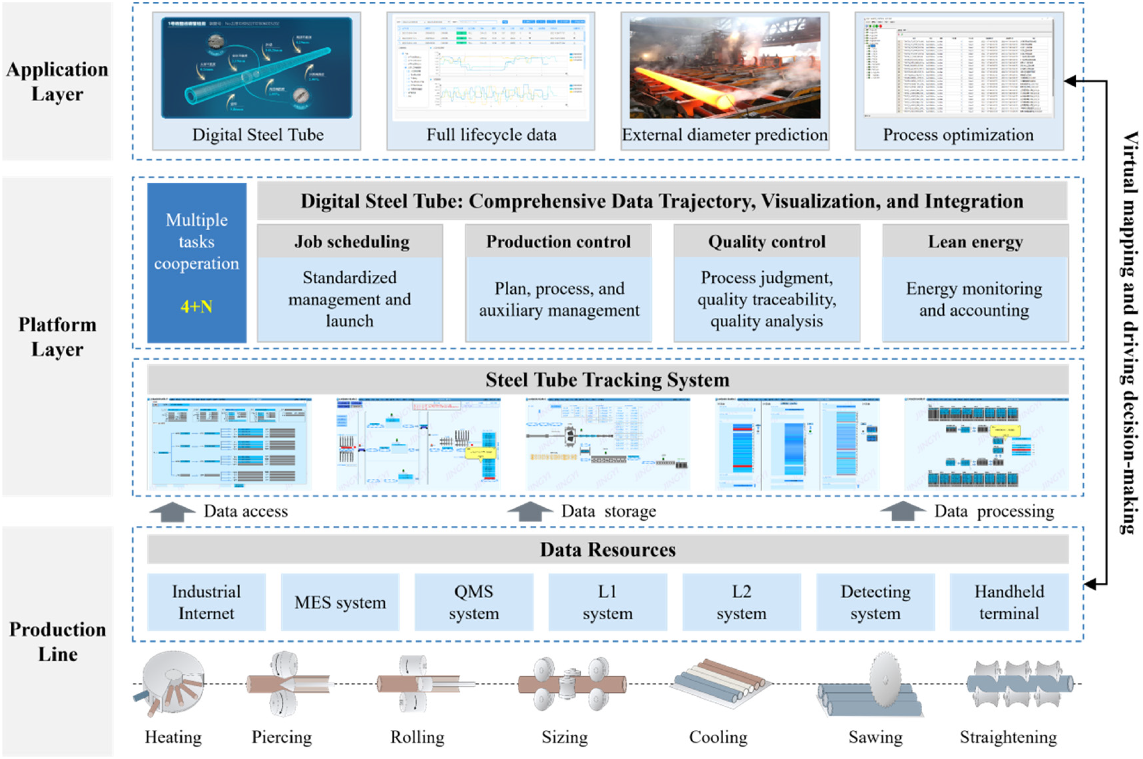
Digital production architecture of the hot-rolled seamless steel tube line.

In addition to the well-established production route, the line is supported by a relatively complete digital management system. A steel tube tracking system enables traceability of individual tubes across multiple process stages and links process parameters, inspection data and production records to the corresponding product unit. Meanwhile, a collaborative platform integrating multiple business functions supports job scheduling, production control, quality control and lean energy management. By integrating information from the industrial internet, the manufacturing execution system, the quality management system, level 1 (L1) and level 2 (L2) systems, inspection systems and handheld terminals, the plant is able to acquire relatively complete and structured production data.

Problem description

Due to the non-uniformity of metal flow during continuous rolling and sizing, the axial deformation of the steel tube is often uneven. This non-uniformity is especially pronounced in the tube end regions, where deformation stability is weaker, and local thickening defects are more likely to occur under unsteady rolling conditions.²⁴ The wall thickness distribution at the head and tail of the tube often deviates significantly from the middle section, leading to an obvious non-uniform axial wall thickness profile. Accurate determination of steel tube wall thickness is essential for quality evaluation and sawing decisions in industrial production. However, on actual production lines, online wall thickness detection is usually available only at limited process stages, and the final wall thickness information often cannot be obtained directly in real time. As a result, timely and effective guidance for subsequent process adjustment is difficult to achieve.

When accurate wall thickness information is unavailable, the determination of sawing allowance often relies on empirical judgment or manual sampling, which is inefficient and cannot accurately reflect the wall thickness distribution of an entire batch of steel tubes. In addition, the wall thickness condition at the tube ends is closely related to the clipped end control process in continuous rolling, but the lack of wall thickness data from subsequent stages makes precise clipped end control difficult. Therefore, improving the prediction accuracy of wall thickness distribution and obtaining wall thickness information in advance are of great practical significance for sawing-position setting, clipped end allowance adjustment and stable control, while also reducing reliance on manual measurement.

Methodology

Datasets and preprocessing

This section presents the dataset construction and preprocessing workflow, including the mechanism basis of wall thickness evolution during multi-stand sizing, variable design, data cleaning and reconstruction, numerical standardisation and dataset partitioning.

Physical metallurgy and sizing mechanism theory

During the sizing process, steel tubes undergo continuous multi-stand thermoplastic deformation. In hot rolling, deformation and temperature evolve simultaneously, and the changing thermal state of the workpiece continuously affects local deformation behaviour.²⁵ Meanwhile, because the corrective capacity of finite passes is limited, the entry wall thickness state may persist and continue to influence the final thickness. Therefore, the sizing process can be regarded as a coupled and continuously evolving system. The core mechanism models are as follows:

Volume conservation model

Under thermoplastic deformation, steel can be approximately treated as an incompressible material. Therefore, for the same metal segment before and after deformation, the relationship between cross-sectional area and axial length can be expressed by the principle of approximate volume conservation²⁶:

A_{in} L_{in} \approx A_{out} L_{out}

(1)

where A_in and A_out represent the cross-sectional areas of the metal before and after sizing, respectively; L_in and L_out denote the lengths of the steel tube before and after sizing.

Pass strain and reduction distribution path model

The sizing process can be viewed as a sequence of continuous multi-pass plastic deformations, and the distribution of deformation among successive stands is critical to metal flow uniformity and final dimensional quality.²⁷ According to the additivity of true strain, the total deformation in a multi-pass process can be expressed as the accumulation of the logarithmic strains introduced by each pass. For the external diameter reduction of the steel tube, the logarithmic reducing rate of the i-th stand can be written as follows:

γ_{i} = \ln (\frac{D_{i - 1}}{D_{i}})

(2)

where D_i₋₁ and D_i are the entry and exit external diameters of the steel tube at the i-th stand, respectively. Accordingly, the total logarithmic reducing rate through all active sizing stands can be expressed as follows:

γ_{tot} = \sum_{i = 1}^{N} γ_{i} = \ln (\frac{D_{0}}{D_{N}})

(3)

where N is the total number of active stands; D₀ and D_N denote the external diameters before and after the whole sizing process, respectively.

Arrhenius-type constitutive model for hot working

During the high-temperature thermoplastic deformation phase of the sizing process, the flow stress of the material is strongly regulated by temperature and strain rate. Among the constitutive approaches used in recent hot working studies, the Arrhenius-type hyperbolic-sine model remains one of the most commonly adopted formulations for describing high-temperature flow behaviour.^28,29 The relationship between the strain rate ε, stress σ and absolute temperature T is expressed by the kinetic rate equation as follows³⁰:

ε = A [\sin h (α σ)]^{n} \exp (- \frac{Q}{R T})

(4)

where A is the structural factor; α is the stress level parameter; n is the stress exponent, reflecting the material's sensitivity to the deformation rate; Q is the activation energy for thermal deformation, characterising the energy required for the material to overcome deformation resistance; R is the molar gas constant; and T is the absolute temperature. By solving for stress as the dependent variable, the expression is derived as follows:

σ = \frac{1}{α} \ln [{(\frac{ε \exp (Q / R T)}{A})}^{1 / n} + \sqrt{{(\frac{ε \exp (Q / R T)}{A})}^{2 / n} + 1}]

(5)

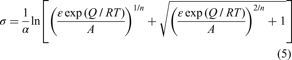
In practical sizing analysis, the strain rate of each pass is usually associated with roll kinematics, deformation zone geometry, and contact conditions. Therefore, rolling speed and deformation geometry should be considered when evaluating the thermoplastic response of the material during the sizing process.³¹

Based on the above mechanism theory, the key parameters influencing the sizing process include the pass deformation path, strain rate effects, geometric deformation intensity, rolling temperature, and the characterisation of entry conditions.

Dataset construction

In this study, modelling and analysis were conducted using online production data from a hot-rolled seamless steel tube production line. During the process, the system synchronously captured process settings and actual operational data related to the sizing stage, alongside critical quality information. This includes, on one hand, online thickness measurements before sizing; and on the other hand, tube geometric specifications and operational parameters for each sizing stand. The wall thickness after sizing was manually recorded using ultrasonic thickness gauges. To quantify the localised deformation during the process, the wall thickness thickening rate was calculated by comparing the measurements before and after sizing. These calculations were performed at 50 mm axial intervals along the tube length. Specifically, the target output of the model is the axial wall-thickening rate sequence [G₂₀₀, G₂₅₀,…, G₈₀₀], which consists of 13 values corresponding to the axial positions from 200 to 800 mm at 50 mm intervals. Each element G_z represents the wall-thickening rate at the axial position z. A total of 131 samples were collected. Given the high dimensionality and significant coupling between parameters, inputting the raw data directly into the model would not only reduce training efficiency but also introduce redundant interference. Therefore, mechanism-based variable selection and structural representation are essential.

Based on the aforementioned physical metallurgy and sizing mechanism theories and related studies,^32,33 the evolution of post-sizing wall thickness is primarily governed by the entry state, geometric and overall deformation intensity, pass schedule profile, and thermomechanical conditions. Accordingly, four categories of input variables were selected: (1) entry wall thickness; (2) geometric and overall deformation indicators, including radial reduction ratio, number of stands, diameter-to-wall ratio, and elongation; (3) pass schedule profile features, represented by statistical and positional descriptors of the normalised reduction distribution, including the mean level, dispersion, peak value and its position, and centre of gravity, to characterise the multi-stand reduction path; and (4) speed schedule profile and thermal condition proxy variables, represented by statistical and positional descriptors of the stand speed distribution, including the mean, fluctuation, extreme values and their positions, and finishing temperature. The input and output features used in the model are listed in Table 1. All variables without units are dimensionless.

Table 1.

The input and output features used in the model.

No	Parameter	Description	Min	Max	Mean
1	X (mm)	Entry wall thickness	6.21	21.21	12.91
2	RC	Radial compression ratio	−0.0044	0.3389	0.1848
3	EL	Elongation ratio	0.9768	1.8958	1.1505
4	DW	Diameter-to-wall ratio	8.5	36.5	13.5
5	Tend	temperature at the sizing exit	821.3	937.0	867.2
6	N	Number of stands	3.0	14.0	8.7
7	Pmean	Mean normalised reduction ratio of active stands	0.0714	0.3334	0.1446
8	Pstd	Standard deviation of reduction distribution	0.0225	0.2062	0.0547
9	Ppeak	Peak normalised reduction ratio of the mill train	0.0974	0.6250	0.2078
10	Ppeakpos	Relative location of the maximum reduction ratio among stands	0.1429	0.6667	0.2892
11	Pcentre	Centroid of the reduction distribution	2.0050	6.5616	4.3396
12	RPMmean (rpm)	Mean roll speeds of active stands	1151.8	1354.1	1245.3
13	RPMstd	Standard deviation of the roll speeds across active stands	1.03	40.99	28.98
14	RPMmin (rpm)	Minimum roll speed	1150.3	1298.0	1245.3
15	RPMmax (rpm)	Max roll speed	1153.3	1421.9	1288.1
16	RPMmaxpos	Location of max roll speed among stands	0.2142	1.0000	0.4339
17	RPMminpos	Location of min roll speed among stands	0.3333	1.0000	0.7676
18	Y (mm)	Exit wall thickness	6.03	23.50	14.31
19	G	Wall thickening rate	0.94	1.45	1.13

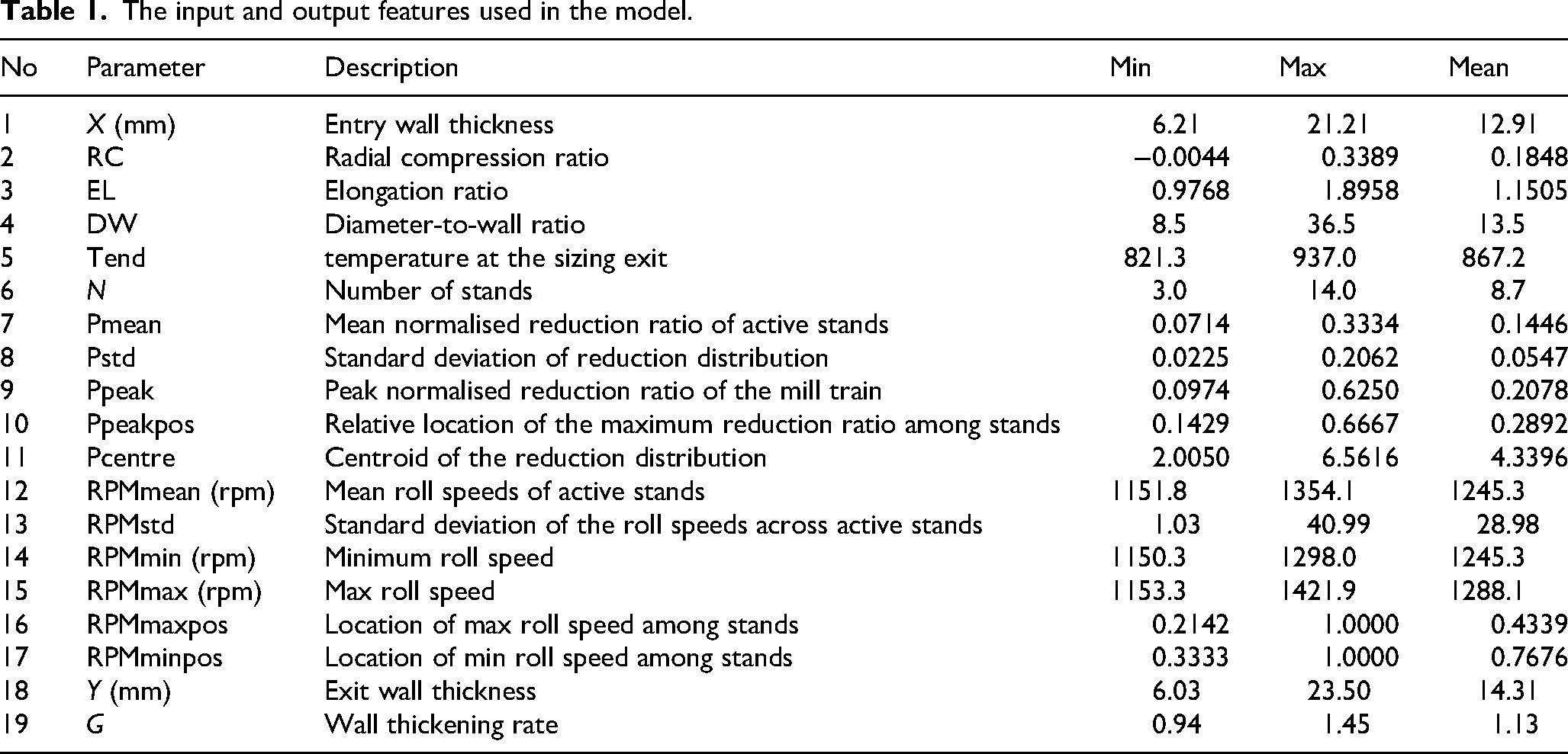
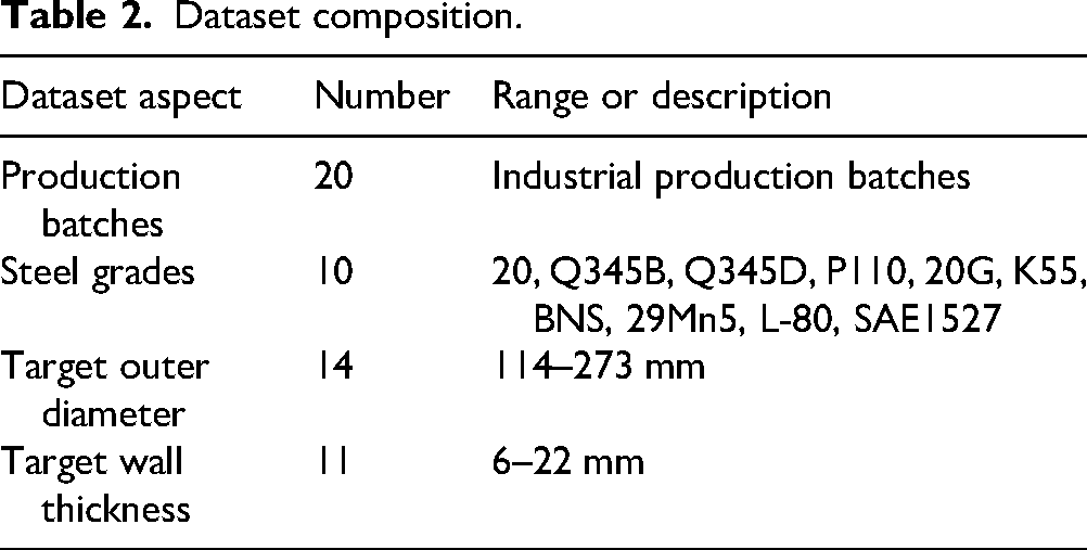
Table 2 summarises the diversity of the industrial dataset. The dataset covers 20 industrial production batches, 10 steel grades, 14 nominal product outer diameter levels and 11 target wall thickness levels.

Table 2.

Dataset composition.

Dataset aspect	Number	Range or description
Production batches	20	Industrial production batches
Steel grades	10	20, Q345B, Q345D, P110, 20G, K55, BNS, 29Mn5, L-80, SAE1527
Target outer diameter	14	114–273 mm
Target wall thickness	11	6–22 mm

To further quantitatively evaluate the linear relationships among the selected features and their correlations with the target variable, Pearson correlation analysis is employed to analyse the input variables and the wall thickening rate vector G. The Pearson correlation coefficient r is calculated as follows³⁴:

r = \frac{\sum_{j = 1}^{n} (x_{j} - \bar{x}) (y_{j} - \bar{y})}{\sqrt{\sum_{j = 1}^{n} {(x_{j} - \bar{x})}^{2}} \sqrt{\sum_{j = 1}^{n} {(y_{j} - \bar{y})}^{2}}}

(6)

where x_j and y_j denote the j-th observed values of variables x and y, respectively;

\bar{x}

and

\bar{y}

represent the mean values of the corresponding variables. The value of r ranges from −1 to 1, where r = 1 indicates a perfect positive correlation, r = −1 indicates a perfect negative correlation, and r = 0 indicates no linear correlation. The results of the Pearson correlation analysis for the selected features are shown in Figure 2. The results indicate that there are significant linear correlations between the input variables and the target variable.

Figure 2.

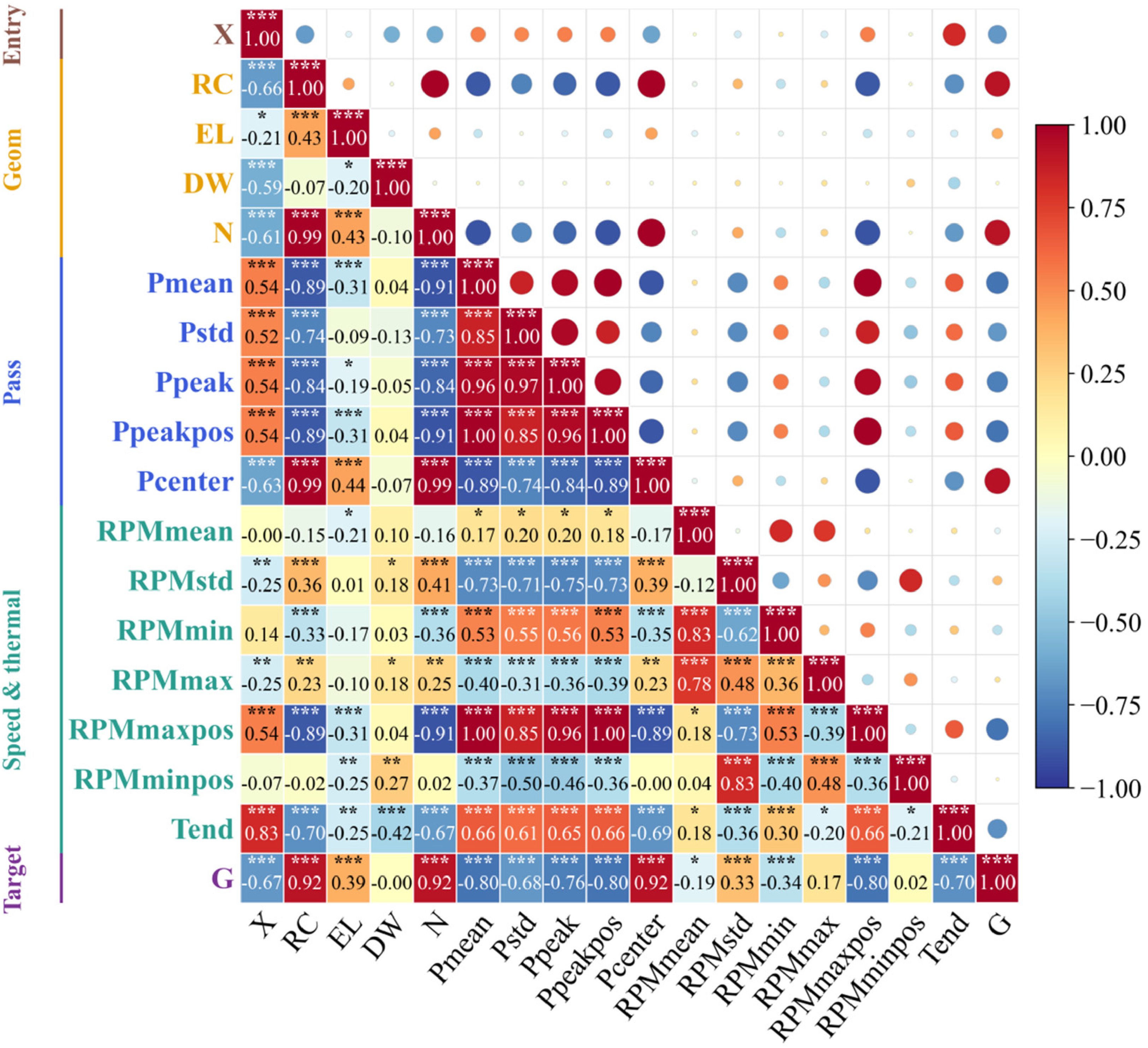
Pearson correlation analysis of variables.

Data reconstruction and cleaning

Because the production data come from multiple sources and differ in dimension, spatial position and representation, unified organisation and preprocessing are required before model construction. In this study, data preprocessing mainly includes four steps: sample alignment, variable calculation, feature construction and numerical normalisation.

Sample alignment and cross-sectional averaging

The wall thickness data before sizing are obtained from the online thickness measurement system, whereas the post-sizing data come from manual ultrasonic measurements. To make the two datasets comparable along the tube axis, both are mapped onto the same discrete axial coordinate sequence at 50 mm intervals, thereby establishing a one-to-one correspondence of wall thickness data along the axial direction.

It should be noted that the number of circumferential measurement channels differs between the online system and the manual ultrasonic measurements. Direct matching between channels is therefore difficult and may introduce additional errors caused by point misalignment and local fluctuations. Therefore, at each axial position z_k, the thickness values from multiple channels within the same cross-section are first averaged circumferentially before subsequent modelling.

The use of circumferential mean values is based on two considerations. First, sizing and reducing processes are intended to improve dimensional precision and suppress circumferential wall thickness eccentricity.³⁵ Thus, the circumferential mean thickness can reasonably represent the main forming effect. Second, the circumferential mean provides a more stable representation of wall thickness evolution by reducing the influence of fluctuations in individual channels while preserving the dominant thickening trend.

Variable calculation

To characterise the local wall thickness variation during the sizing process, the wall thickening rate vector G is calculated based on the thickness values at corresponding positions before and after sizing. This variable reflects the local thickness response of the material during the sizing process and serves as the core predictive target in the subsequent modelling.

Feature construction

To avoid the high dimensionality and redundant information introduced by directly using raw multi-stand process parameters, this study represents the sizing-related profiles in terms of a set of low-dimensional and interpretable functional descriptors. For the pass schedule information, normalised reduction distribution features are constructed, including the mean, standard deviation, peak value, peak position and centre of gravity of the reduction amounts across active stands as statistical descriptors. Regarding the roll speed information, the mean, standard deviation, minimum, maximum and their respective positions within the speed distribution are constructed. For geometric deformation features, the radial reduction ratio, number of stands, diameter-to-wall ratio and elongation are retained. Additionally, the tube temperature at the sizing exit is incorporated into the model inputs as a characterisation variable for the thermal state.

Outlier Detection

To improve the reliability of the sample data, the isolation forest algorithm was used for outlier detection. Isolation forest is an unsupervised anomaly detection method based on random partitioning, in which anomalous samples are more likely to be isolated with shorter path lengths than normal samples. The anomaly score can be expressed as follows³⁶:

s (x, n) = 2^{- \frac{E [h (x)]}{c (n)}}

(7)

where s(x,n) is the anomaly score of sample x; E(h(x)) is the average path length of the sample in an isolation tree; and c(n) is the path length normalisation factor for n samples. A higher anomaly score implies a higher probability that the sample is an outlier.

In this study, the number of trees was set to 300, the maximum number of samples was automatically determined according to the dataset size, the contamination rate was set to 0.02, and the random seed was fixed at 1. The detection results are shown in Figure 3, where normal and abnormal samples are marked by white circles and red squares, respectively. Since the output variable G is a high-dimensional vector composed of thickening rates at multiple positions, only a representative example is presented for visualisation. Specifically, G_{200 mm} and G_{800 mm} were selected to construct a two-dimensional single tube space. As shown in Figure 3, most normal samples are concentrated in the main dense region, indicating that the majority of samples exhibit similar characteristics in the single tube space, whereas the abnormal samples are distributed outside this region and deviate from the dominant sample pattern. From the initial 131 samples, three abnormal samples were identified and removed, leaving 128 valid samples for subsequent modelling and analysis.

Figure 3.

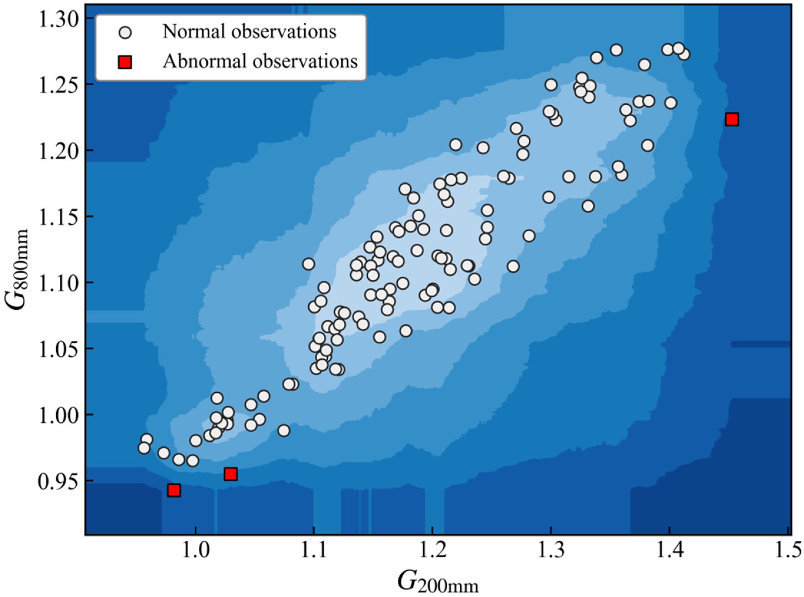
Isolation forest outlier detection with outlier areas.

Numerical normalisation

Given the significant differences in dimensions and numerical ranges among various input and target variables, directly feeding them into the model would compromise the stability of the parameter optimisation process. To mitigate the adverse effects of scale disparities, this study employs a standardisation method based on the mean and standard deviation of the training set. For any variable x, the standardisation formula is as follows:

x^{'} = \frac{x - μ_{train}}{σ_{train}}

(8)

where μ_train and σ_train denote the mean and standard deviation of the variable within the current fold of the training set, respectively. Their calculation formulas are as follows:

μ_{train} = \frac{1}{N_{train}} \sum_{j = 1}^{N_{train}} x_{j}

(9)

σ_{train} = \sqrt{\frac{1}{N_{train}} \sum_{j = 1}^{N_{train}} {(x_{j} - μ_{train})}^{2}}

(10)

where N_train is the number of samples in the training set; x_j represents the value of the variable for the j-th sample in the training set.

Dataset partition and cross-validation strategy

Given the relatively limited sample size, a random five-fold cross-validation strategy was adopted to improve data utilisation and evaluation robustness. All samples were first divided into five folds. In each iteration, one fold was used as the test set, and the remaining four folds were further split into the training set and validation set at a ratio of 8:2.

The random seed was fixed at 42 to ensure reproducibility. Thus, the test set accounted for ∼20% of the total samples in each fold. To avoid data leakage, normalisation parameters were fitted only on the training set and then applied to the corresponding validation and test sets. Final model performance was obtained by aggregating the results of all five folds.

Model constructed strategy

1D-CNN algorithm

1D-CNN is well-suited for ID sequence modelling because it can extract local features and variation patterns through local connections and weight sharing, while reducing the number of model parameters and preserving local structural information.³⁷ Therefore, it is particularly suitable for sequence prediction tasks with local dependencies.

1D-CNN extracts local features by sliding convolutional kernels across the input sequence. Let the input sequence be $X = [x_{1}, x_{2}, \dots, x_{n}]$ , then the output of the convolutional layer can be represented as follows³⁸:

h_{t} = f [\sum_{m = 1}^{k} w_{m} x_{(t + m - 1)} + b]

(11)

where h_t denotes the convolution output at the t-th position; k denotes the kernel size; w_m denotes the convolution kernel parameters; b denotes the bias term; and f(·) denotes the activation function.

After the convolutional layer, a pooling layer is introduced to compress and filter the convolutional features, thereby reducing the feature dimension and eliminating redundant information. The output of the pooling layer can be expressed as:

p_{t} = p o o l (h_{t : t + s - 1})

(12)

where pool(·) denotes the pooling function; s represents the pooling window size; and p_t denotes the output feature after pooling.

The pooled features are fed into fully connected layers to establish the mapping relationship between the extracted features and the target output, which can be expressed as follows:

y = g (W h + b)

(13)

where h denotes the feature vector obtained after convolution and pooling; W and b represent the weights and bias of the fully connected layer, respectively; g(·) denotes the output function; and y represents the final predicted value.

During training, network parameters are updated by backpropagation to minimise the prediction error. For the regression task in this study, the mean squared error (MSE) is adopted as the loss function as follows:

L = \frac{1}{N} \sum_{j = 1}^{N} (y_{j} - {\hat{y}}_{j})^{2}

(14)

where N denotes the number of samples; y_j represents the ground truth and

\hat{y_{j}}

represents the predicted value.

The proposed model consists of two ID convolution layers with kernel size 3 and output channels of 32 and 64, respectively, and each convolution layer is followed by a ReLU activation function. An adaptive average pooling layer is then used to compress the feature map while retaining the main information. The pooled feature vector is concatenated with other scalar features and fed into a fully connected module composed of three linear layers, in which the first two layers use ReLU activation and the final layer outputs the prediction result.

This two-branch structure was designed to ensure that convolution is applied only to physically ordered data rather than to an arbitrary vector of heterogeneous process variables. Specifically, the before-sizing wall-thickness sequence [X₂₀₀, X₂₅₀,…, X₈₀₀] is used as the convolutional input, with adjacent elements corresponding to neighbouring axial positions of the same tube at 50 mm intervals. Because these neighbouring positions are physically correlated during multi-stand sizing, the 1D convolution can capture local axial dependencies and fluctuation patterns. The remaining process descriptors are normalised as an auxiliary scalar feature vector and concatenated with the pooled axial features, and the combined vector is then fed into fully connected layers to output the 13-dimensional wall-thickening rate sequence.

1D-CNN optimised by PSO

To improve the computational efficiency and predictive accuracy of the model, an appropriate optimisation algorithm is required for efficient hyperparameter selection.³⁹ To further improve the predictive performance of the 1D-CNN model, PSO is employed to optimise its key hyperparameters. As a stochastic optimisation method based on swarm intelligence, PSO is suitable for nonlinear multi-parameter optimisation because of its simple implementation and strong global search capability. In PSO, each particle represents a candidate hyperparameter combination, whose position and velocity denote the current solution and its update direction, respectively. During optimisation, each particle updates itself according to both its personal best position and the global best position of the swarm. The velocity and position update rules are given by the following equations⁴⁰:

v_{u}^{(t + 1)} = ω v_{u}^{t} + c_{1} r_{1} (p_{u}^{t} - x_{u}^{t}) + c_{2} r_{2} (g^{t} - x_{u}^{t})

(15)

x_{u}^{(t + 1)} = x_{u}^{t} + v_{u}^{(t + 1)}

(16)

where

x_{u}^{t}

and

v_{u}^{t}

denote the position and velocity of the u-th particle at the t-th iteration, respectively; ω represents the inertia weight; c₁ and c₂ are the cognitive and social learning factors, respectively; r₁ and r₂ are random numbers within the interval [0,1];

p_{u}^{t}

denotes the individual historical best position of the particle, and g_t represents the current global best position of the swarm.

In this study, PSO is utilised to optimise the learning rate, weight decay coefficient, hidden layer dimensions, dropout ratio, batch size, training epochs and early stopping parameters of the 1D-CNN to enhance both predictive accuracy and generalisation ability. For each set of candidate parameters generated by the particle swarm, a corresponding 1D-CNN model is constructed. The average validation error from five-fold cross-validation is then employed as the fitness value. The optimisation objective is to minimise the five-fold average MSE, expressed as follows:

F i t n e s s = \frac{1}{K} \sum_{q = 1}^{K} {MSE}_{q}

(17)

where K denotes the number of cross-validation folds, which is set to 5 in this study. By continuously updating the positions and velocities of the particles, the optimal hyperparameter combination is eventually obtained, upon which the PSO-1D-CNN model is established. The specific process of optimising the 1D-CNN using PSO is illustrated in Figure 4.

Step 1: Preprocess the raw dataset and complete feature extraction, normalisation, and data partitioning.

Step 2: Initialise the particle swarm to generate multiple sets of candidate hyperparameters for the 1D-CNN.

Step 3: Construct and train 1D-CNN models based on the parameter combinations represented by the particles, using the average of the five-fold validation errors as the particle fitness.

Step 4: Update the velocity and position of the particles based on their individual best positions and the swarm's global best position.

Step 5: Repeat the iterative process until the preset number of searches is reached.

Step 6: Output the global optimal hyperparameter combination and establish the final PSO-1D-CNN model accordingly.

Figure 4.

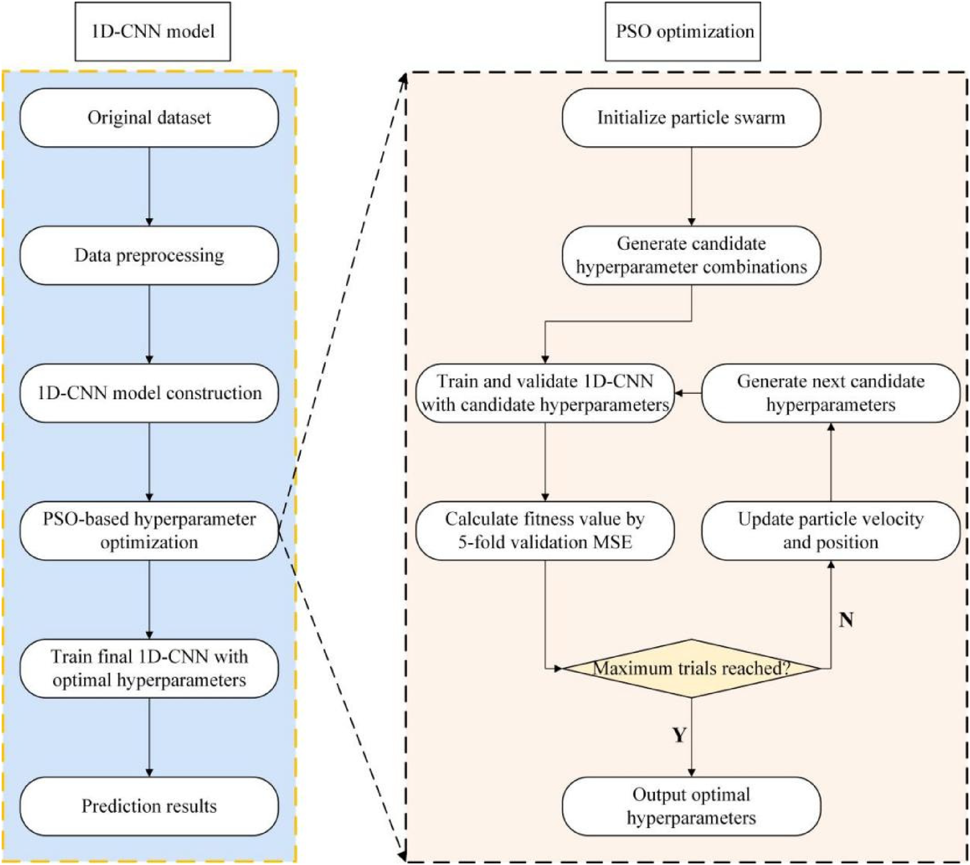
Particle swarm optimisation and one-dimensional convolutional neural network (PSO-1D-CNN) prediction model framework.

Comparison of different models

Furthermore, five predictive models were selected for comparative analysis, including the conditional variational autoencoder (CVAE), multi-layer perceptron (MLP), light gradient boosting machine (LightGBM), extreme gradient boosting (XGBoost) and categorical boosting (CatBoost). Among them, MLP is a representative feedforward neural network that has been widely used in rolling process modelling and manufacturing quality prediction because of its ability to approximate complex nonlinear mappings between process variables and product responses.⁴¹ XGBoost, LightGBM and CatBoost are representative tree ensemble models based on boosting, which are also commonly adopted in rolling and metallurgical process prediction due to their strong nonlinear fitting ability and robust performance on structured industrial data.⁴² CVAE was introduced because it can learn the overall curve shape and local variation characteristics through conditional distribution modelling.^43,44

The performance of these models is evaluated by the root mean square error (RMSE), the coefficient of determination (R²), and the MAE between the observed and predicted thickening rate. Their calculation formulas are as follows:

RMSE = \sqrt{\frac{1}{N} \sum_{i = 1}^{N} {(Y_{i} - {\hat{Y}}_{i})}^{2}}

(18)

R^{2} = 1 - \frac{\sum_{i = 1}^{N} {(Y_{i} - {\hat{Y}}_{i})}^{2}}{\sum_{i = 1}^{N} {(Y_{i} - {\hat{Y}}_{)}}^{2}}

(19)

MAE = \frac{1}{N} \sum_{i = 1}^{N} | Y_{i} - {\hat{Y}}_{i} |

(20)

where N denotes the number of samples; Y_i and $\hat{Y_{i}}$ represent the observed and predicted values for the i-th sample, respectively; and $\bar{Y}$ represents the mean of the observed values. Smaller values of RMSE and MAE indicate lower predictive errors, while an R² value closer to 1 signifies superior fitting performance.

SHAP interpretability analysis method

SHAP is a post-hoc interpretation method based on cooperative game theory. This method quantifies the contribution of each input feature to the model's prediction by assigning a Shapley value, thereby providing global and local explanations for complex black-box models. Within the SHAP framework, a model prediction can be expressed as an additive combination of individual feature contributions:

g (x) = ϕ_{0} + \sum_{k = 1}^{M} ϕ_{k}

(21)

where M denotes the number of input features; ϕ₀ represents the baseline value of the model output and ϕ_k denotes the Shapley value corresponding to the k-th feature. A positive ϕ_k indicates that the feature increases the predicted value, while a negative ϕ_k indicates that it decreases the predicted value. The Shapley value is calculated by averaging the marginal contributions of a feature across all possible subsets of features, as follows:

ϕ_{k} = \sum_{S \subseteq F ∖ {k}} \frac{| S |! (| F | - | S | - 1)!}{| F |!} [f (S \cup j) - f (S)]

(22)

where F denotes the complete set of features, and S represents a feature subset that does not include feature k.

In this study, the SHAP method is employed for the interpretive analysis of the PSO-1D-CNN model. Since the model predicts a 13-dimensional axial wall-thickening rate sequence [G₂₀₀, G₂₅₀,…, G₈₀₀], corresponding to the axial positions from 200 to 800 mm at 50 mm intervals, the SHAP values are first calculated separately for all output positions and then aggregated. Specifically, the mean absolute SHAP values are used for global feature importance ranking, while the signed average SHAP values across the 13 output positions are utilised for feature contribution direction analysis, local sample explanation and dependence analysis.

Results and discussion

Model hyperparameter settings

Hyperparameter settings have a substantial impact on model accuracy, training stability and generalisation ability. Because different models vary in architecture, parameter scale and training mechanism, their performance is often highly sensitive to hyperparameter configurations. Therefore, to reduce the randomness of manual tuning and ensure a fair comparison, systematic hyperparameter optimisation was performed for all models. Sparrow search algorithm (SSA), Harris hawks optimisation (HHO), and PSO were adopted as the hyperparameter optimisation methods.

To ensure the fairness of the comparison, hyperparameter tuning was applied to all models, including XGBoost, LightGBM, CatBoost, CVAE, MLP and 1D-CNN. All models were optimised under the same data partitioning and validation protocol, and their overall performance was evaluated using Taylor diagrams. The comparative results obtained using different hyperparameter optimisation algorithms are presented in Figure 5, where panels (a) to (c) correspond to SSA, HHO and PSO, respectively.

Figure 5.

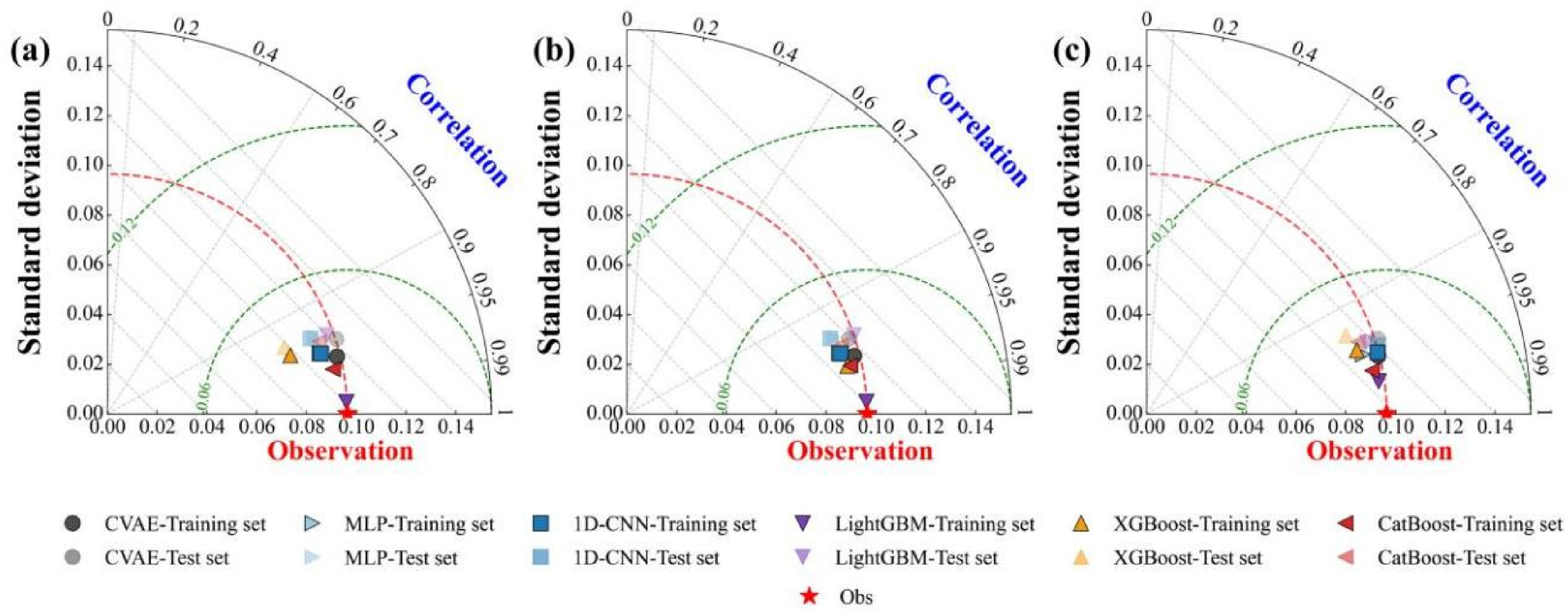
Taylor diagram analysis of model performance: (a) sparrow search algorithm (SSA), (b) Harris hawks optimisation (HHO) and (c) particle swarm optimisation (PSO).

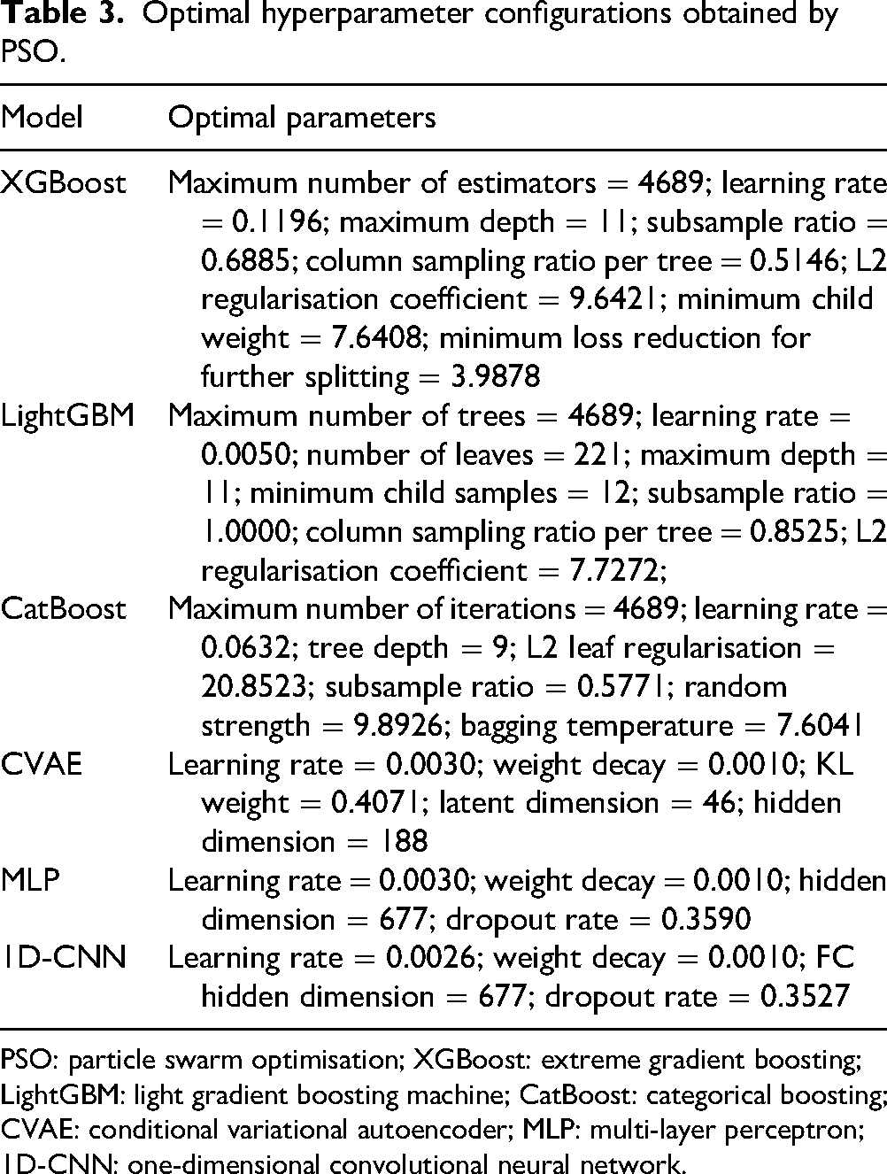
The Taylor diagrams reveal clear differences among the three optimisation algorithms. For SSA, the model points are relatively scattered and show noticeable separation between the training and test sets, indicating limited stability and weaker generalisation. Although HHO improves the overall distribution to some extent, several models still exhibit visible train-test deviations. In contrast, the PSO-optimised models are generally located closer to the observation reference, with more consistent standard deviations, higher correlations and smaller gaps between training set and test set. This indicates that PSO achieves a more balanced optimisation effect and better generalisation performance. Therefore, PSO was selected as the final hyperparameter optimisation algorithm in this study. SSA was not selected because its results were relatively scattered and unstable, implying a higher risk of overfitting. HHO was not selected because its overall train-test consistency was still weaker than that of PSO. The optimal hyperparameters of each model obtained by PSO are summarised in Table 3. These configurations were used in the subsequent training and performance evaluation.

Table 3.

Optimal hyperparameter configurations obtained by PSO.

Model	Optimal parameters
XGBoost	Maximum number of estimators = 4689; learning rate = 0.1196; maximum depth = 11; subsample ratio = 0.6885; column sampling ratio per tree = 0.5146; L2 regularisation coefficient = 9.6421; minimum child weight = 7.6408; minimum loss reduction for further splitting = 3.9878
LightGBM	Maximum number of trees = 4689; learning rate = 0.0050; number of leaves = 221; maximum depth = 11; minimum child samples = 12; subsample ratio = 1.0000; column sampling ratio per tree = 0.8525; L2 regularisation coefficient = 7.7272;
CatBoost	Maximum number of iterations = 4689; learning rate = 0.0632; tree depth = 9; L2 leaf regularisation = 20.8523; subsample ratio = 0.5771; random strength = 9.8926; bagging temperature = 7.6041
CVAE	Learning rate = 0.0030; weight decay = 0.0010; KL weight = 0.4071; latent dimension = 46; hidden dimension = 188
MLP	Learning rate = 0.0030; weight decay = 0.0010; hidden dimension = 677; dropout rate = 0.3590
1D-CNN	Learning rate = 0.0026; weight decay = 0.0010; FC hidden dimension = 677; dropout rate = 0.3527

PSO: particle swarm optimisation; XGBoost: extreme gradient boosting; LightGBM: light gradient boosting machine; CatBoost: categorical boosting; CVAE: conditional variational autoencoder; MLP: multi-layer perceptron; 1D-CNN: one-dimensional convolutional neural network.

To further examine the overfitting risk under the limited-sample condition, the training and validation loss curves of the six models were recorded, as shown in Figure 6. For the neural-network-based models, including PSO-1D-CNN, PSO-MLP and PSO-CVAE, the curves are plotted against training epochs, whereas for the tree-ensemble models, including PSO-LightGBM, PSO-XGBoost and PSO-CatBoost, they are plotted against boosting iterations. The number of estimators, trees or iterations reported in Table 3 represent the PSO-optimised maximum training limits, while the final effective model size was determined by validation-loss-based early stopping.

Figure 6.

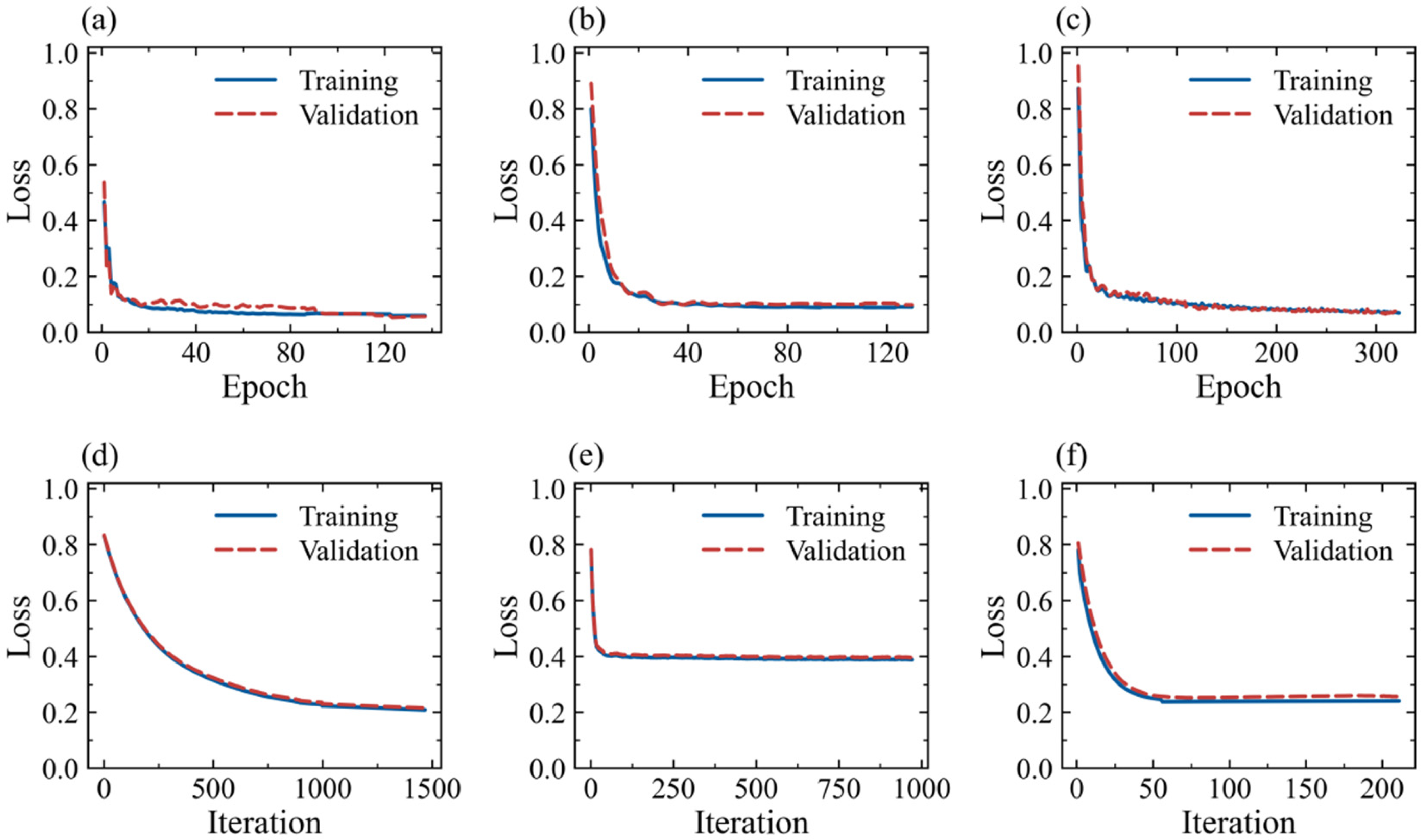
Training and validation loss curves of different models: (a) PSO-1D-CNN, (b) PSO-MLP, (c) PSO-CVAE, (d) PSO-LightGBM, (e) PSO-XGBoost, and (f) PSO-CatBoost.

As shown in Figure 6, the training and validation losses of the proposed PSO-1D-CNN decrease rapidly at the early stage and then converge to a stable level, without obvious divergence between the two curves. Similar convergence behaviour is also observed for the benchmark models, although PSO-MLP and PSO-CVAE show certain validation fluctuations. For the tree-ensemble models, the validation loss becomes stable before reaching the maximum boosting limit, indicating that early stopping helps prevent unnecessary model growth.

Model-specific regularisation and overfitting-control strategies were adopted to reduce the risk of memorising the limited samples. For the neural-network-based models, dropout, L2 weight decay, validation-loss-based early stopping and learning-rate scheduling were used, while gradient clipping was applied to improve training stability. For PSO-CVAE, the KL-divergence term further regularised the latent distribution. For the tree-ensemble models, overfitting was controlled by depth or leaf-size constraints, column sampling, subsampling, L2 regularisation, split-gain constraints and validation-loss-based early stopping where applicable.

Model predictions and analysis

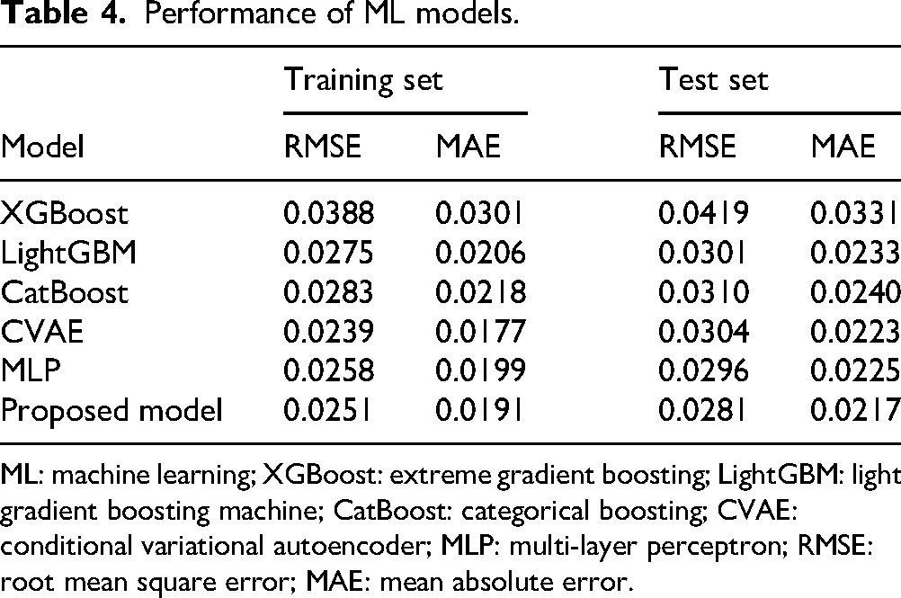
Table 4 summarises the prediction performance of different models on the training and test sets using the optimal hyperparameters determined by PSO. RMSE and MAE were used to evaluate predictive accuracy. On the test set, the proposed model achieves the best overall performance, with the lowest RMSE (0.0281) and MAE (0.0217). MLP and CVAE also show competitive results, with RMSE values of 0.0296 and 0.0304 and MAE values of 0.0225 and 0.0223 on the test set, respectively.

Table 4.

Performance of ML models.

Model	Training set		Test set
Model	RMSE	MAE	RMSE	MAE
XGBoost	0.0388	0.0301	0.0419	0.0331
LightGBM	0.0275	0.0206	0.0301	0.0233
CatBoost	0.0283	0.0218	0.0310	0.0240
CVAE	0.0239	0.0177	0.0304	0.0223
MLP	0.0258	0.0199	0.0296	0.0225
Proposed model	0.0251	0.0191	0.0281	0.0217

ML: machine learning; XGBoost: extreme gradient boosting; LightGBM: light gradient boosting machine; CatBoost: categorical boosting; CVAE: conditional variational autoencoder; MLP: multi-layer perceptron; RMSE: root mean square error; MAE: mean absolute error.

A comparison between the training and test results further reflects the generalisation characteristics of each model. Although CVAE achieves the lowest training errors, its performance degrades more noticeably on the test set, suggesting a larger generalisation gap. By comparison, the proposed model maintains relatively low errors on both the training and test sets, indicating a better balance between fitting ability and generalisation performance.

The scatter plots of observed versus predicted values in Figure 7 provide an intuitive visual comparison of the predictive performance of the six models on the training and test sets. As shown in Figure 7(a), among the six models, XGBoost exhibits the most dispersed scatter distribution, and its fitted line deviates more obviously from the 1:1 reference line, particularly on the test set. Combined with its relatively low test set R² value of 0.8045 and the higher error metrics reported in Table 4, this result suggests that XGBoost is less effective in capturing the complex nonlinear relationships involved in the current task. LightGBM and CatBoost perform better than XGBoost, with more concentrated point distributions and improved alignment between the fitted lines and the ideal reference line, although noticeable dispersion still exists in certain value ranges. MLP and CVAE also show relatively compact point distributions and good consistency between the fitted lines and the reference line, indicating competitive predictive capability. However, compared with the proposed model, their scatter clouds are slightly more dispersed, especially on the test set. As shown in Figure 7(f), the proposed model exhibits the most concentrated sample distribution, with most points on both the training and test sets closely clustered around the 1:1 line. Its fitted lines are highly consistent with the ideal reference line, indicating strong fitting stability and generalisation ability. This observation is further supported by its highest R² value of 0.913 and the lowest RMSE and MAE on the test set, as reported in Table 4.

Figure 7.

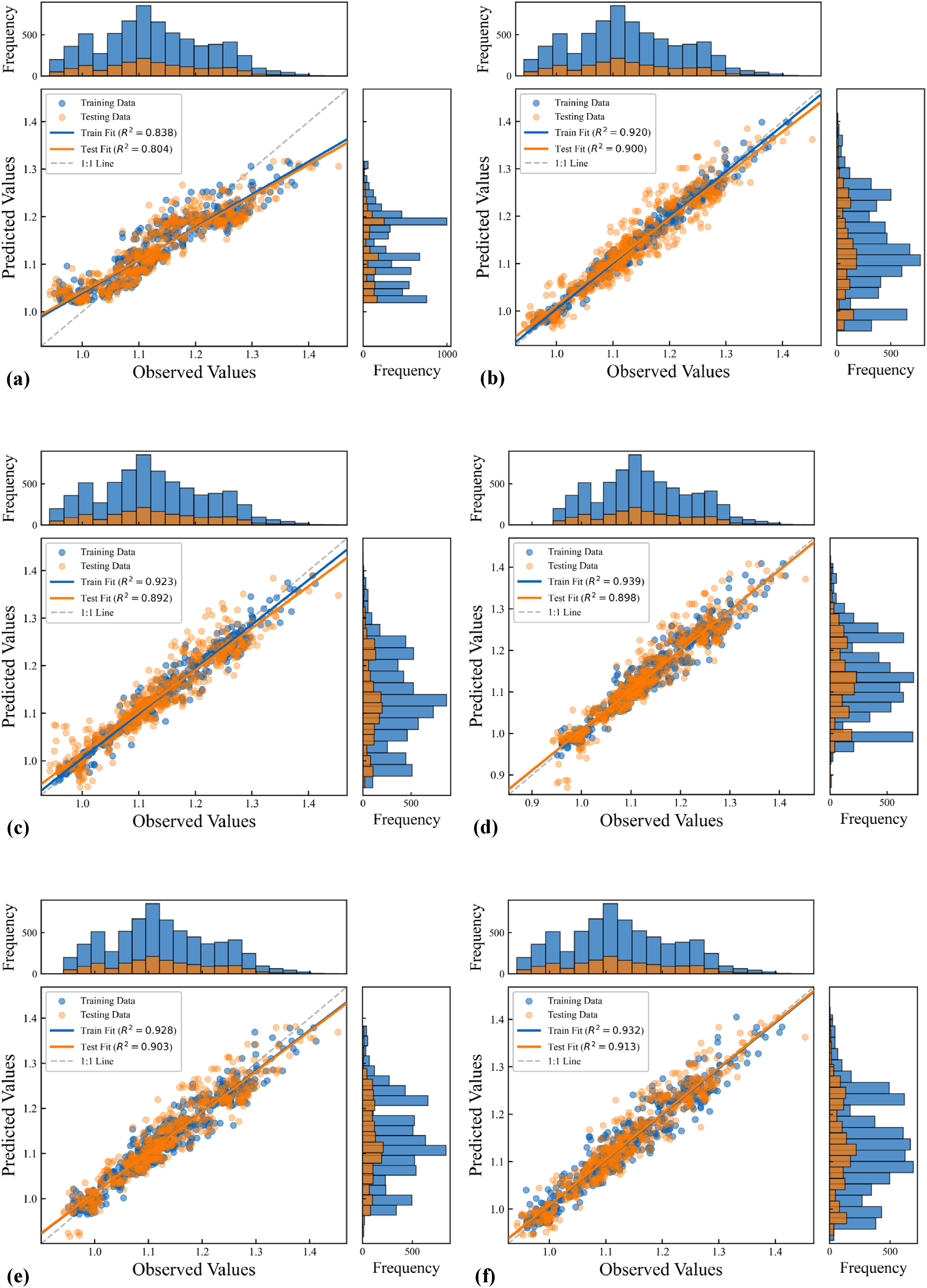
Model prediction results: (a) XGBoost, (b) LightGBM, (c) CatBoost, (d) CVAE, (e) MLP and (f) proposed model.

Considering that random cross-validation may overestimate model performance when similar product specifications are shared between training and test folds, a specification-grouped cross-validation experiment was further conducted to assess industrial generalisation more strictly. In this experiment, samples were grouped according to product specifications, defined by the nominal outer diameter and nominal wall thickness. During data partitioning, samples belonging to the same specification group were assigned to the same fold, so that the same specification would not appear simultaneously in the training and test sets. Compared with random five-fold cross-validation, this setting provides a stricter evaluation of the model's ability to generalise to different specification conditions.

The results are summarised in Table 5. Compared with the random five-fold cross-validation results, the performance of all models decreases under the specification-grouped setting, which is expected because the similarity between training and test samples is reduced. Nevertheless, the proposed PSO-1D-CNN still achieves the best performance among all compared models, with the highest R² of 0.7850, the lowest MAE of 0.0247 and the lowest RMSE of 0.0322. In addition, compared with the benchmark models, the proposed model exhibits a relatively smaller decrease in performance under the specification-grouped validation setting, indicating that it is less sensitive to the stricter grouped data partitioning strategy. These results demonstrate that PSO-1D-CNN not only achieves the highest prediction accuracy under the specification-grouped validation strategy, but also maintains better performance stability when evaluated under more challenging industrial generalisation conditions.

Table 5.

Specification-grouped cross-validation results.

Model	R ²	MAE	RMSE
LightGBM	0.6372	0.0297	0.0382
XGBoost	0.6437	0.0322	0.0413
CatBoost	0.6499	0.0328	0.0390
CVAE	0.6628	0.0337	0.0400
MLP	0.7218	0.0286	0.0361
Proposed model	0.7850	0.0247	0.0322

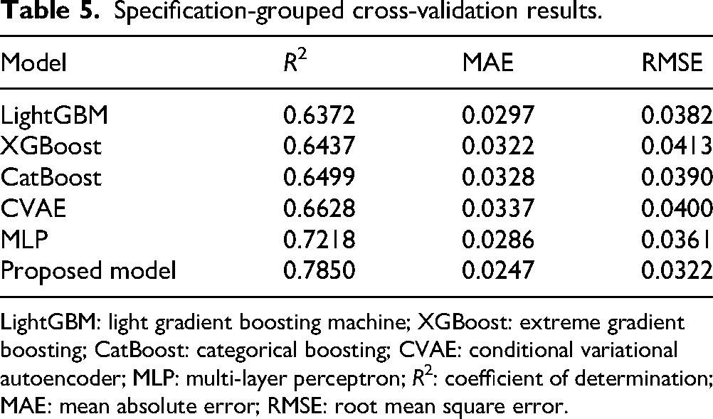
LightGBM: light gradient boosting machine; XGBoost: extreme gradient boosting; CatBoost: categorical boosting; CVAE: conditional variational autoencoder; MLP: multi-layer perceptron; R²: coefficient of determination; MAE: mean absolute error; RMSE: root mean square error.

To further evaluate the robustness of the proposed PSO-1D-CNN under the limited-sample condition, a repeated random-seed stability analysis was conducted. The PSO-optimised hyperparameters were kept unchanged, and ten repeated five-fold cross-validation experiments were performed using different random split seeds. For each repetition, the complete five-fold training and testing procedure was repeated, and the averaged test-set metrics were recorded. The statistical results are summarised in Table 6.

Table 6.

Repeated random-seed cross-validation results.

Metric	Mean	Std	Min	Max
R ²	0.8966	0.0131	0.8686	0.9128
MAE	0.0229	0.0010	0.0217	0.0250
RMSE	0.0298	0.0015	0.0280	0.0333

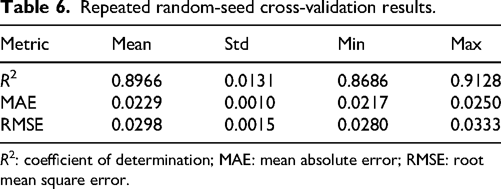
R²: coefficient of determination; MAE: mean absolute error; RMSE: root mean square error.

As shown in Table 6, the proposed PSO-1D-CNN achieved an average R² of 0.8966 ± 0.0131, an MAE of 0.0229 ± 0.0010 and an RMSE of 0.0298 ± 0.0015 across 10 repeated experiments. The R² values ranged from 0.8686 to 0.9128, indicating that the proposed model maintains relatively stable predictive performance under different random data partitions. These results provide additional evidence for the robustness and generalisation ability of the PSO-1D-CNN in the limited-sample setting.

Model interpretability analysis

Global SHAP analysis of model predictions

To interpret the decision logic of the PSO-1D-CNN and quantify the influence of key inputs, SHAP was used for global interpretation, as shown in Figure 8. Figure 8(a) presents the global feature importance ranked by mean absolute SHAP value, and Figure 8(b) shows the distribution and direction of feature contributions across all samples. Larger mean absolute SHAP values indicate stronger overall effects, while the bee swarm plot reflects contribution direction and sample heterogeneity.

Figure 8.

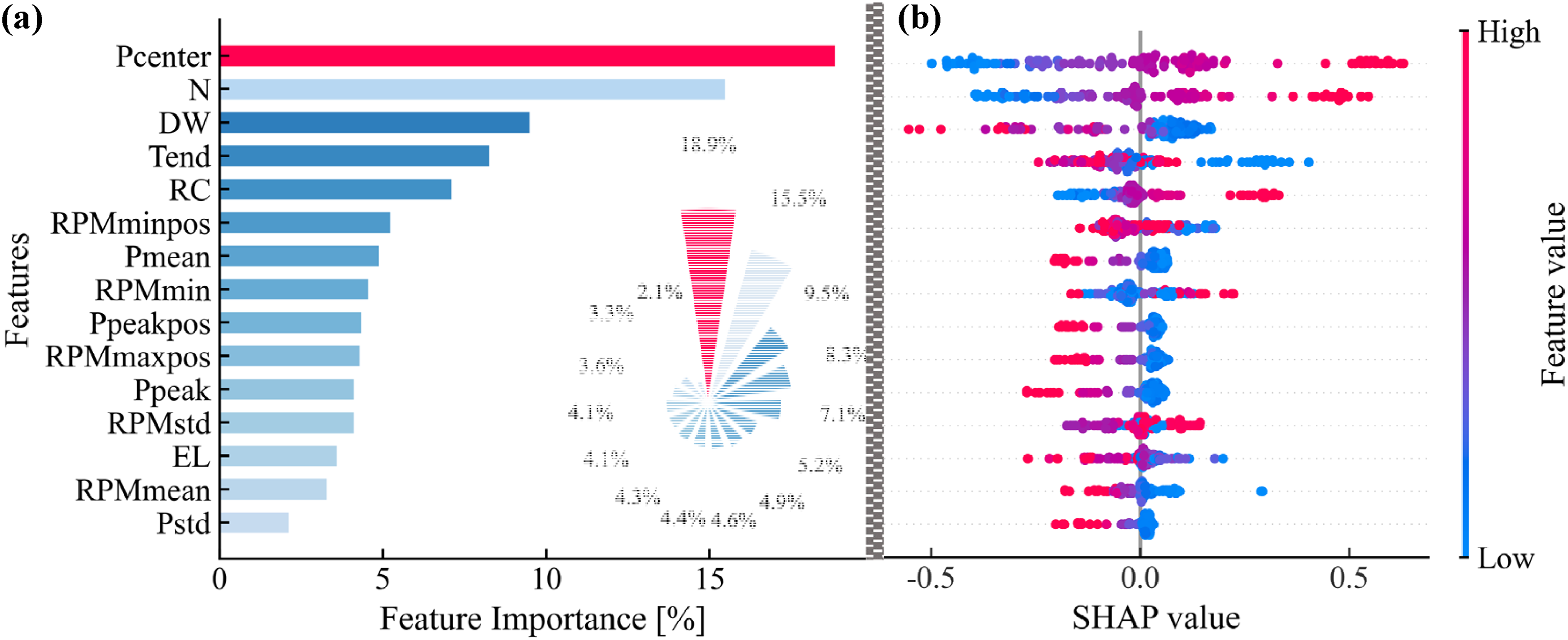
Analysis of the importance of model input features: (a) the average SHapley Additive exPlanations (SHAP) absolute values and (b) the SHAP value distribution.

As shown in Figure 8(a), Pcentre, N, DW, Tend and RC are the five most important variables, indicating that the model is mainly governed by the reduction distribution path, active stand configuration, dimensional matching, tube temperature at the sizing exit and radial compression ratio. This is consistent with the established sizing mechanism. Among them, Pcentre ranks first, suggesting that the centroid of the reduction distribution plays a dominant role in prediction. This dominant role can be further interpreted from the viewpoint of axial metal-flow redistribution and the volume-conservation framework introduced earlier. Pcentre represents the centroid position of the normalised reduction distribution along the active sizing stands, reflecting whether the main diameter-reduction deformation is concentrated in the upstream or downstream part of the sizing mill. A shift in this reduction centroid changes the distribution of radial compression and inter-stand tensile deformation along the rolling direction, thereby affecting axial metal-flow redistribution. As described by the volume-conservation relationship in equation (1), radial compression, axial elongation and wall-thickness evolution are coupled during thermoplastic sizing. Therefore, the high SHAP importance of Pcentre indicates that the model captures a physically meaningful mechanism: the spatial allocation of reduction across stands strongly influences axial metal redistribution and consequently affects the final wall-thickness thickening profile. Meanwhile, the high importance of N indicates that the number of stands strongly affects deformation partitioning.

In addition, DW and RC rank third and fifth, respectively. From the perspective of volume conservation, diameter reduction, wall thickness redistribution, and axial elongation are coupled during thermoplastic sizing. Accordingly, DW reflects the dimensional matching condition and generally shows a negative contribution at higher values, whereas RC characterises radial compression ratio and tends to contribute positively when its value is high. Tend also shows high importance, confirming that tube temperature at the sizing exit significantly affects the prediction in a manner consistent with the hot working constitutive relationship. As shown in Figure 8(b), higher Tend values are mainly associated with negative or SHAP values close to zero, whereas lower values tend to correspond to positive contributions. Other variables also contribute to the prediction, although their effects are relatively weaker.

Local SHAP analysis of model predictions

To further explain the model's prediction process at the individual sample level, two representative samples were selected for local SHAP analysis, as shown in Figure 9. In the figure, red arrows indicate features that exert a positive contribution to the prediction result, while blue arrows represent features with a negative contribution. The length of the arrows reflects the magnitude of each feature's contribution to the final predicted value. As illustrated in the figure, the cumulative contribution of all input variables starts from the baseline value E[f(X)] and ultimately yields the predicted result f(x) corresponding to the sample.

Figure 9.

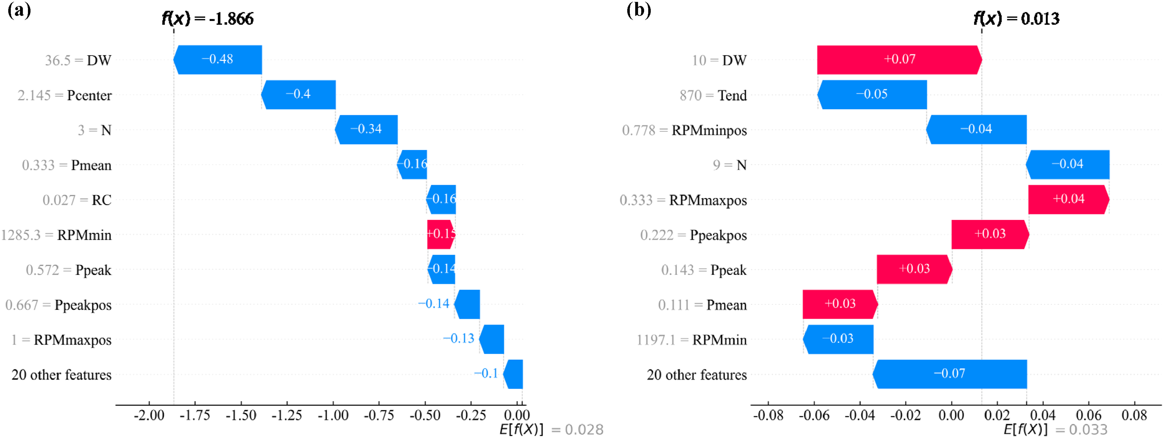
Waterfall analysis of different individual samples: (a) random Sample a and (b) random Sample b.

As shown in Figure 9(a), Sample a is mainly dominated by negative contributions. Among all variables, DW, Pcentre and N are the most influential features, and all of them significantly reduce the predicted value. Other features, including Pmean, RC, Ppeak, Ppeakpos and RPMmaxpos, also contribute negatively, whereas RPMmin provides only limited positive effects and does not alter the overall negative trend.

By contrast, Sample b in Figure 9(b) shows a more balanced contribution pattern. DW, RPMmaxpos, Ppeakpos, Ppeak, and Pmean contribute positively, while Tend, RPMminpos, N and RPMmin show negative effects. Comparing the two samples indicates that the same feature may exhibit different contribution directions and magnitudes under different conditions. For example, DW has a strong negative contribution in Sample a but a positive contribution in Sample b, indicating that its effect on the model output is value-dependent rather than fixed. Similar sample-dependent behaviour can also be observed for other variables.

SHAP-based feature relationship analysis

SHAP-based relationship plots of the top nine variables ranked by global SHAP importance are presented in Figure 10. These relationships further clarify the specific impacts of various process conditions on the wall thickening rate during the sizing process, and reveal that there are positive correlation, negative correlation or nonlinear response characteristics between different variables and the model output.

Figure 10.

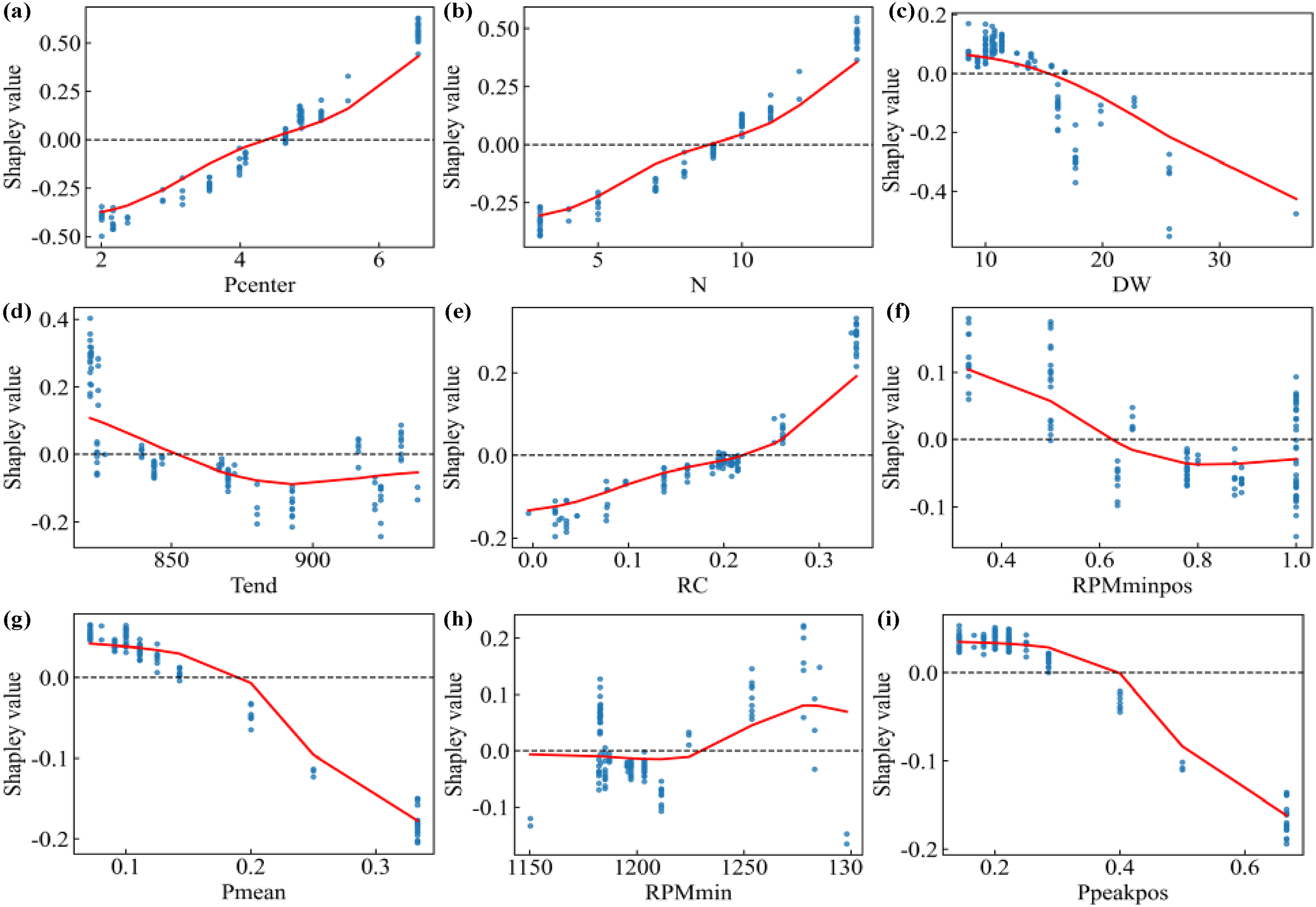
SHapley Additive exPlanations (SHAP)-based relationships between key features and model predictions.

As illustrated in Figure 10, Pcentre, N and RC generally exhibit a positive relationship with the model output. This indicates that the backward shift of the centroid of the reduction distribution, the increase in the number of stands, and the enhancement of the radial compression ratio are overall more likely to increase the wall thickening rate predicted by the model. In contrast, DW shows an obvious negative correlation trend: as DW increases from ∼10 to 38, the corresponding SHAP value decreases from about 0.08 to −0.45, demonstrating that a larger diameter-to-wall ratio is generally unfavourable for improving the wall thickening rate. Pmean and Ppeakpos also present relatively distinct negative response characteristics, indicating that a higher average reduction distribution level and the backward shift of the peak position are more likely to correspond to negative contributions within the current sample range. For Tend, its SHAP value decreases more significantly in the middle interval, showing an overall trend of first decreasing and then levelling off.

Industrial application

Figure 11 presents the online application interface of the wall thickness prediction and sawing decision system deployed on an industrial seamless steel tube rolling line. The prediction model has been integrated into the production system, enabling real-time prediction of the axial wall thickness profile for each steel tube during operation. Based on the predicted wall thickness curve and the tolerance limits specified by the production order, the system further predicts the sawing length for the selected tube. The interface directly displays the prediction results together with key process parameters, thereby providing operators with intuitive production information and quantitative support for decisions.

Figure 11.

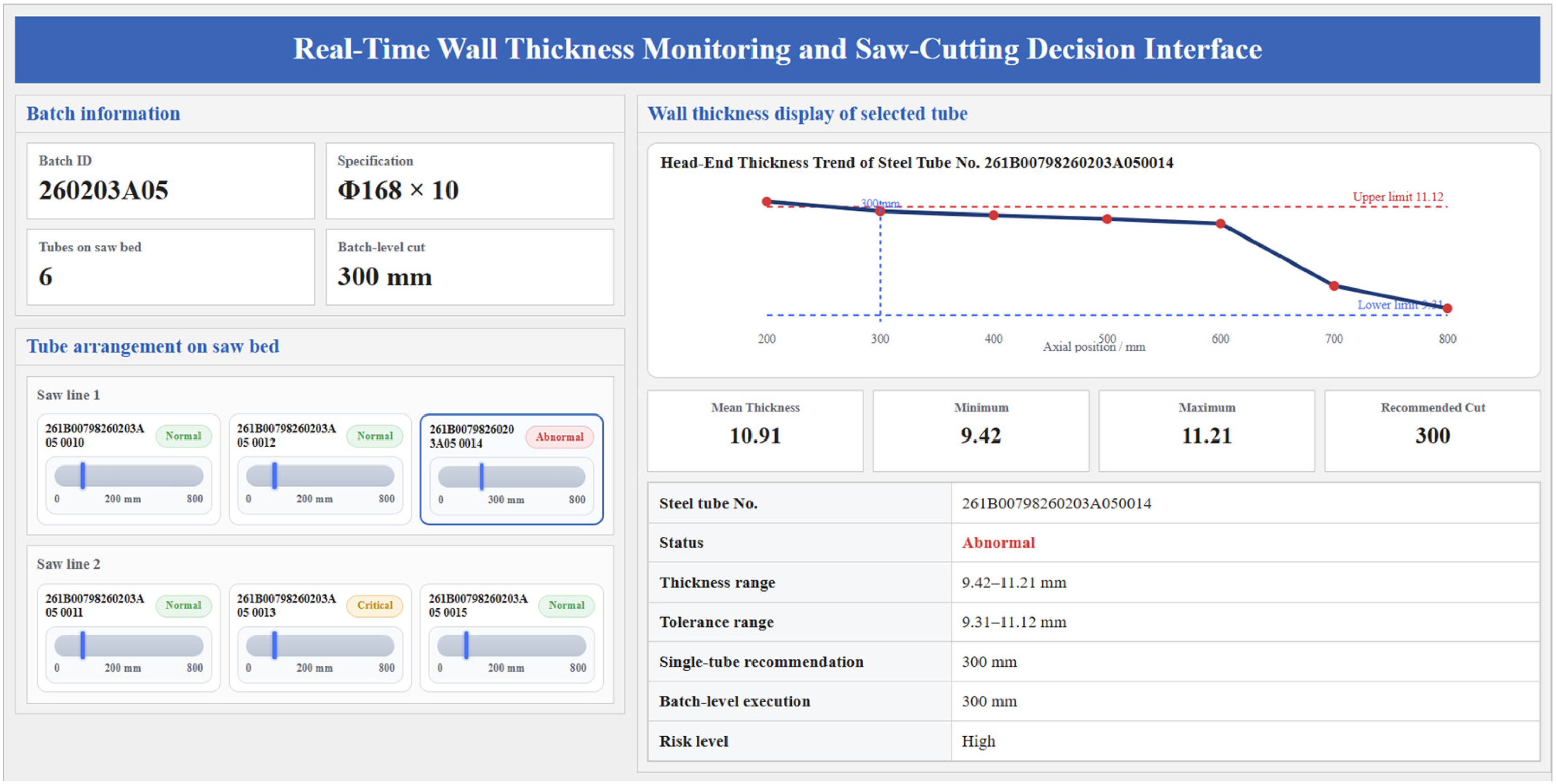
Online application interface of the wall thickness prediction system deployed on an industrial seamless steel tube rolling line.

In addition, the interface integrates three types of information, namely batch information, the real-time display of steel tubes on the saw bed, and the predicted wall thickness of the selected tube. This design enables operators to simultaneously identify the predicted cut length of the selected tube and the execution value adopted at the batch level. In this way, the system establishes an effective link between model prediction and sawing decisions, providing data support for production adjustment and operational control while reducing reliance on empirical manual judgment.

Conclusions

This study addresses two practical challenges in hot-rolled seamless steel tube production: the lack of online access to post-sizing axial wall thickness information and the reliance on empirical sawing decisions. A prediction model for the post-sizing axial single tube distribution was developed using field measurement data and evaluated in terms of predictive performance, interpretability, and industrial applicability. The main conclusions are as follows:

The sizing process is governed by the coupling of entry wall thickness, geometric and overall deformation indicators, pass schedule profile features, speed schedule profile and thermal conditions, resulting in a highly nonlinear axial single tube distribution. Predicting this distribution is therefore important for process quality control and accurate sawing decisions.

Among the compared ML and DL models, PSO-1D-CNN achieved the best predictive performance. On the test set, the model obtained an RMSE of 0.0281, MAE of 0.0217 and R² of 0.913, demonstrating good accuracy, stability and generalisation ability for industrial applications.

SHAP analysis shows that the centroid of the reduction distribution, the number of stands, the diameter-to-wall ratio, the tube temperature at the sizing exit and the radial reduction ratio are the key factors affecting prediction, which is consistent with the sizing mechanism. The model has also been integrated into an online system for real-time thickness prediction, sawing parameter calculation and batch visualisation, reducing reliance on empirical judgment.

Future work will focus on expanding the dataset to cover more specifications, steel grades and operating conditions, while further strengthening the integration of mechanism-guided and data-driven methods to support coordinated thickness prediction, sawing optimisation, and process control toward online closed-loop optimisation.

Footnotes

Acknowledgements

The research work is supported by the National Key Research and Development Plan (Grant No. 2023YFB3712404).

ORCID iDs

Xiao-chen Wang

Jin-bo Zhou

Funding

The authors disclosed receipt of the following financial support for the research, authorship, and/or publication of this article: This work was supported by the National Key Research and Development Program of China (grant number 2023YFB3712404).

Declaration of conflicting interests

The authors declared no potential conflicts of interest with respect to the research, authorship, and/or publication of this article.

References

Chen

Zhang

, et al. Online cooling system and improved similar self-adaptive strategy for hot-rolled seamless steel tube. ISIJ Int 2021; 61: 2135–2142.

, et al. Small data machine learning in materials science. NPJ Comput Mater 2023; 9: 42.

Bertolini

Mezzogori

Neroni

, et al. Machine learning for industrial applications: a comprehensive literature review. Expert Syst Appl 2021; 175: 114820.

Ekonomou

Fotis

Maris

, et al. Estimation of the electromagnetic field radiating by electrostatic discharges using artificial neural networks. Simul Model Pract Theory 2007; 15: 1089–1102.

Fotis

Ekonomou

Maris

, et al. Development of an artificial neural network software tool for the assessment of the electromagnetic field radiating by electrostatic discharges. IET Sci Meas Technol 2007; 1: 261–269.

Meng

Ding

, et al. Novel shape control system of hot-rolled strip based on machine learning fused mechanism model. Expert Syst Appl 2024; 255: 124789.

Ding

Lei

, et al. An interpretable framework for high-precision flatness prediction in strip cold rolling. J Mater Process Technol 2024; 329: 118452.

Ding

, et al. Predicting hot-strip finish rolling thickness using stochastic configuration networks. Inf Sci (NY) 2022; 611: 677–689.

Dong

Luan

, et al. Fusion of theory and data-driven model in hot plate rolling: a case study of rolling force prediction. Expert Syst Appl 2024; 245: 123047.

10.

Meng

Ding

Dong

, et al. A novel modelling method for rolling force prediction based on deep stochastic configuration networks fused with physical knowledge. Inf Sci (NY) 2025; 711: 122097.

11.

Shang

Chen

Sun

, et al. High-precision rolling force prediction for hot rolling based on multimodal physical information and reinforcement learning. J Manuf Process 2025; 151: 655–678.

12.

Dong

Cui

, et al. Rolling theory-guided prediction of hot-rolled plate width based on parameter transfer strategy. ISA Trans 2024; 146: 352–365.

13.

Cui

Cao

, et al. Physical metallurgy guided deep learning for yield strength of hot-rolled steel based on the small labeled dataset. Mater Des 2022; 223: 111269.

14.

Langbauer

Nunner

Zmek

, et al. Development of an artificial neural network (ANN) model to predict the temperature of hot-rolled steel pipes. Adv Ind Manuf Eng 2022; 5: 100090.

15.

Langbauer

Nunner

Zmek

, et al. Modelling of thermal shrinkage of seamless steel pipes using artificial neural networks (ANN) focusing on the influence of the ANN architecture. Results Eng 2023; 17: 100999.

16.

Chen

Sun

Wang

, et al. Rolling theory-guided prediction of PQF mill rolling force based on DE-GWO-BP. Ironmak Steelmak 2026; 53: 611–620.

17.

Huang

Zhou

. Research on strip crown by uncertain sampling strategy modified particle swarm optimization with RBF neural network. Appl Soft Comput 2022; 130: 109661.

18.

Jeon

Seo

Jung

, et al. Prediction and mechanism explain of austenite-grain growth during reheating of alloy steel using XAI. J Mater Res Technol 2022; 21: 1408–1418.

19.

Sai

Rathore

Chauhan

. Machine learning-based predictions of fatigue life for multi-principal element alloys. Scr Mater 2023; 226: 115214.

20.

Wang

, et al. Interpretable machine learning modeling of alloy composition-process-property relationships based on industrial big data in hot strip rolling. J Manuf Process 2025; 150: 299–316.

21.

Sun

Wang

, et al. Application of novel interpretable machine learning framework for strip flatness prediction during tandem cold rolling. Measurement (Mahwah NJ) 2025; 244: 116516.

22.

Wen

, et al. A mechanism and data fusion step-wise prediction framework for hot-rolled strip thickness. J Manuf Process 2025; 134: 680–696.

23.

Jiang

Tang

, et al. Explicit FE modelling of tube stretch reduction and analysis of wall thickness variation. Ironmak Steelmak 2015; 42: 176–184.

24.

Zhang

. Energy method in stretch reducing process of steel tube. J Iron Steel Res Int 2008; 15: 39–43.

25.

Komori

. Simulation of deformation and temperature in caliber rolling: effect of finite-element mesh in cross-section. J Mater Process Technol 2003; 143-144: 367–372.

26.

Hosford

Caddell

. Metal forming: mechanics and metallurgy. Cambridge: Cambridge University Press, 2011.

27.

Yang

Huang

, et al. A new correction theory and verification on the reducing rate distribution for seamless tube stretch-reducing process. Crystals (Basel) 2022; 12: 1296.

28.

Alaneme

Kareem

Bodunrin

. Hyperbolic–sine constitutive model determined hot deformation mechanisms and workability response of Al–Zn/Cu and Al–Zn/SiC based composites. Results Eng 2023; 19: 101255.

29.

Liu

Yin

, et al. Investigation into the thermal deformation behavior and the establishment of a constitutive relationship for Mn-Cr-Ni-Mo steel. Mater Technol 2024; 58: 503–510.

30.

Sellars

McTegart

. On the mechanism of hot deformation. Acta Metall 1966; 14: 1136–1138.

31.

Bayoumi

. Analysis of flow and stresses in a tube stretch-reducing hot rolling schedule. Int J Mech Sci 2003; 45: 553–565.

32.

Pan

Tao

Zhang

, et al. Deep learning methods utilization in mechanical property of medium-Mn steel. Steel Res Int 2024; 95: 2400243.

33.

Hou

Wang

, et al. Weldability of high entropy alloys: microstructure, mechanical property, and corrosion resistance. J Manuf Process 2023; 99: 209–229.

34.

Wang

Zeng

, et al. Machine learning for prediction of retained austenite fraction and optimization of processing in quenched and partitioned steels. J Iron Steel Res Int 2024; 31: 2002–2013.

35.

Jiang

. Method for improving transverse wall thickness precision of seamless steel tube based on tube rotation. J Iron Steel Res Int 2015; 22: 924–930.

36.

Hariri

Kind

Brunner

. Extended isolation forest. IEEE Trans Knowl Data Eng 2021; 33: 1479–1489.

37.

Liu

Yang

, et al. A survey of convolutional neural networks: analysis, applications, and prospects. IEEE Trans Neural Netw Learn Syst 2022; 33: 6999–7019.

38.

Ince

Kiranyaz

Eren

, et al. Real-time motor fault detection by 1-D convolutional neural networks. IEEE Trans Ind Electron 2016; 63: 7067–7075.

39.

Pan

. Bayesian Optimization+ XGBoost based life cycle carbon emission prediction for residential buildings—an example from Chengdu, ChinaBuilding simulation. Beijing: Tsinghua University Press, 2023, pp.1451–1466.

40.

Kennedy

Eberhart

. Particle swarm optimization Proceedings of ICNN'95-international conference on neural networks. 4. Piscataway, NJ: IEEE, 1995, pp.1942–1948.

41.

Ding

Wang

, et al. A novel cost-sensitive quality determination framework in hot rolling steel industry. Inf Sci (NY) 2024; 678: 121054.

42.

Ding

Sun

, et al. A high-precision and transparent step-wise diagnostic framework for hot-rolled strip crown. J Manuf Syst 2023; 71: 144–157.

43.

Sohn

Lee

Yan

. Learning structured output representation using deep conditional generative models. Adv Neural Inf Process Syst 2015; 28: 3483–3491.

44.

Balmer

Kuhn

Bischof

, et al. Design space exploration and explanation via conditional variational autoencoders in meta-model-based conceptual design of pedestrian bridges. Autom Constr 2024; 163: 105411.