ViTA: A flexible CAD-tool-independent automatic grading platform for two-dimensional CAD drawings

Abstract

Grading engineering drawings takes a significant amount of an instructor’s time, especially in large classrooms. In many cases, teaching assistants help with grading, adding levels of inconsistency and unfairness. To help in grading automation of CAD drawings, this paper introduces a novel tool that can completely automate the grading process after students submit their work. The introduced tool, called Virtual Teaching Assistant (ViTA), is a CAD-tool-independent platform that can work with exported drawings originating from different CAD software having different export settings. Using computer vision techniques applied to exported images of the drawings, ViTA can not only recognize whether or not a two-dimensional (2 D) drawing is correct, but also offers the detection of many important orthographic and sectional view mistakes such as mistakes in structural features, outline, hatching, orientation, scale, line thickness, colors, and views. We show ViTA’s accuracy and its relevance in the automated grading of 2 D CAD drawings by evaluating it using 500 student drawings created with three different CAD software.

Keywords

Autograder CAD 2D drawings computer vision

Introduction

The number of assignments to be graded increases with the number of students. This makes the manual CAD grading process time consuming, resulting in delayed feedback to students. Motivated to overcome these drawbacks and enhance students’ learning experience, we develop a tool for automated grading of 2 D engineering drawings. We call this tool the Virtual Teaching Assistant, or ViTA in short. ViTA helps reducing grading time of 2 D CAD drawings by introducing a set of tools that the grader can use. Depending on their grading rubric, the grader can use some or all of ViTA’s features and assign appropriate grading criteria to the correct/incorrect drawing features. ViTA can detect whether or not a drawing is correct, and it can currently detect mistakes in its structural features, outline, hatching, orientation, scale, line thickness, colors, and views.

A key feature of ViTA – differentiating itself from the existing tools – is that it is completely independent of the CAD software used by the students (and the instructor) to create the drawing. ViTA can work with drawings originating from multiple CAD tools with different export settings. It achieves that through the use of a computer-vision-based analysis of the drawings. This feature gives the students the freedom of choosing to work with a CAD software that they are already familiar with, without the need to learn how to use a specific CAD software associated with the course.

In addition to saving significant grading time and eliminating the possibility of human error related to the manual grading of drawings, ViTA could potentially be embedded in various online learning management systems for CAD courses – in engineering graphics, architecture, etc. – for automatic grading. It can also be used to give feedback to the students on their drawings and the nature of the feedback can be determined by the instructor.

The remainder of this paper is organized as follows. The Background Section presents a background for this work. The Virtual Teaching Assistant Section discusses ViTA in detail. ViTA is then evaluated in the Evaluation Section. The Conclusion and Future Work Section concludes this work and presents directions for future work.

Background

Various computer programs have been developed to compare technical drawings and highlight the differences between two drawings. The following summarizes the most relevant ones and presents their shortcomings.

Autodesk, the company behind some of the most popular CAD tools, has a plug-in called “Drawing Compare” for AutoCAD Architecture that compares two drawings.¹ It was developed using Application Program Interface (API) programming. The plug-in works, in simple terms, as if a drawing on a tracing paper is placed on the original or correct drawing and these two drawings are then compared. The differences in the two drawings are then highlighted using different colors and labels. Among the first to propose using the API system were Guerci and Baxter, who outlined a method by which instructors could compare a student-submitted work to a reference document using the API data in SolidWorks Visual Basic.² An example of the original drawings to compare is shown in Figure 1 and the resulting comparison is shown in Figure 2. The Drawing Compare plug-in, although useful in comparing drawings, has some disadvantages. The plug-in shows the differences between two drawings temporarily, and the comparison results cannot be saved. Furthermore, the plug-in can only be used for drawings having the same scale; it does not work for drawings with variable scale and different orientations. It could also conclude that a whole drawing is wrong even if it only has one small mistake. In addition, this plug-in is only available for AutoCAD files.

Figure 1.

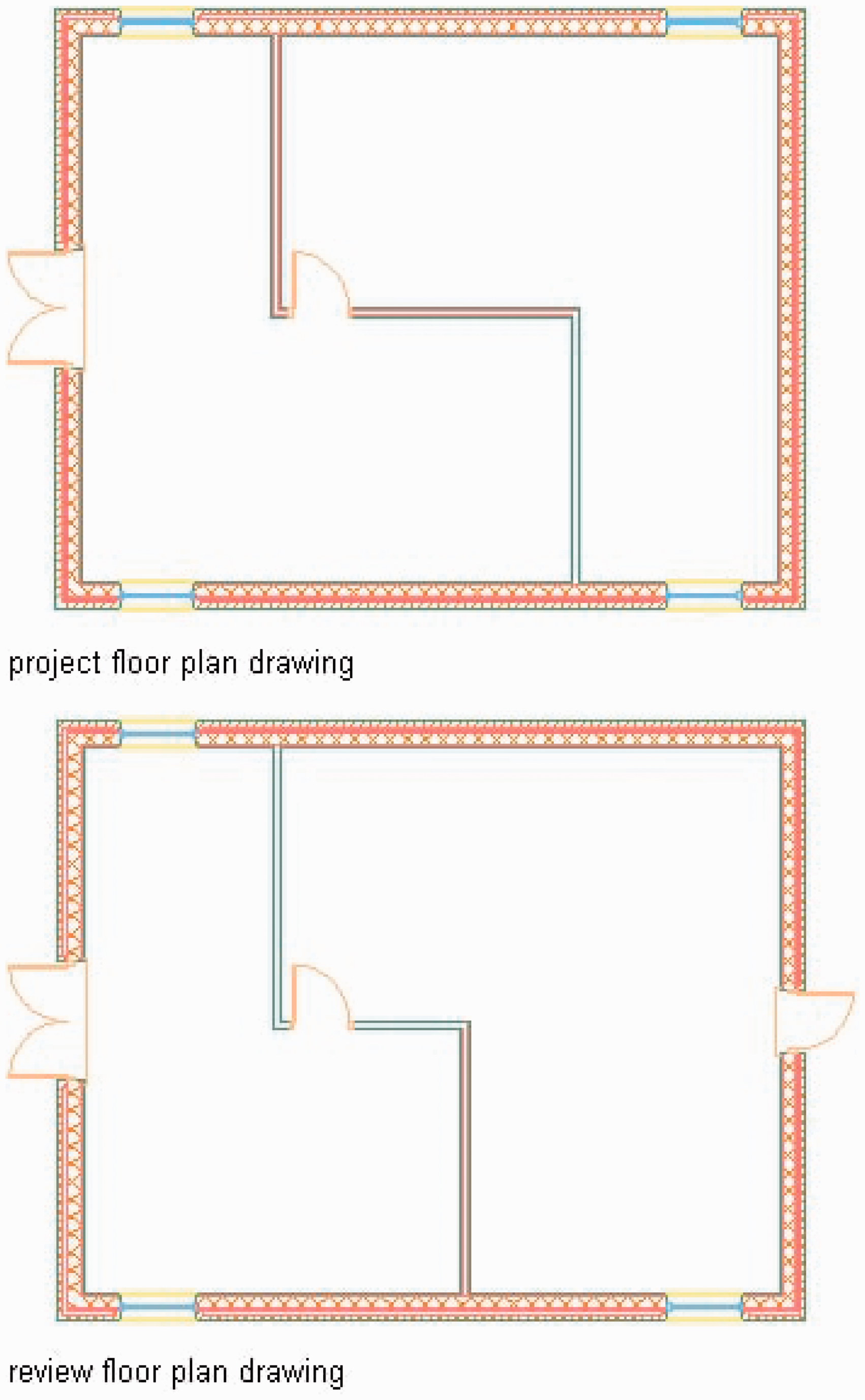
Drawings to compare.

Figure 2.

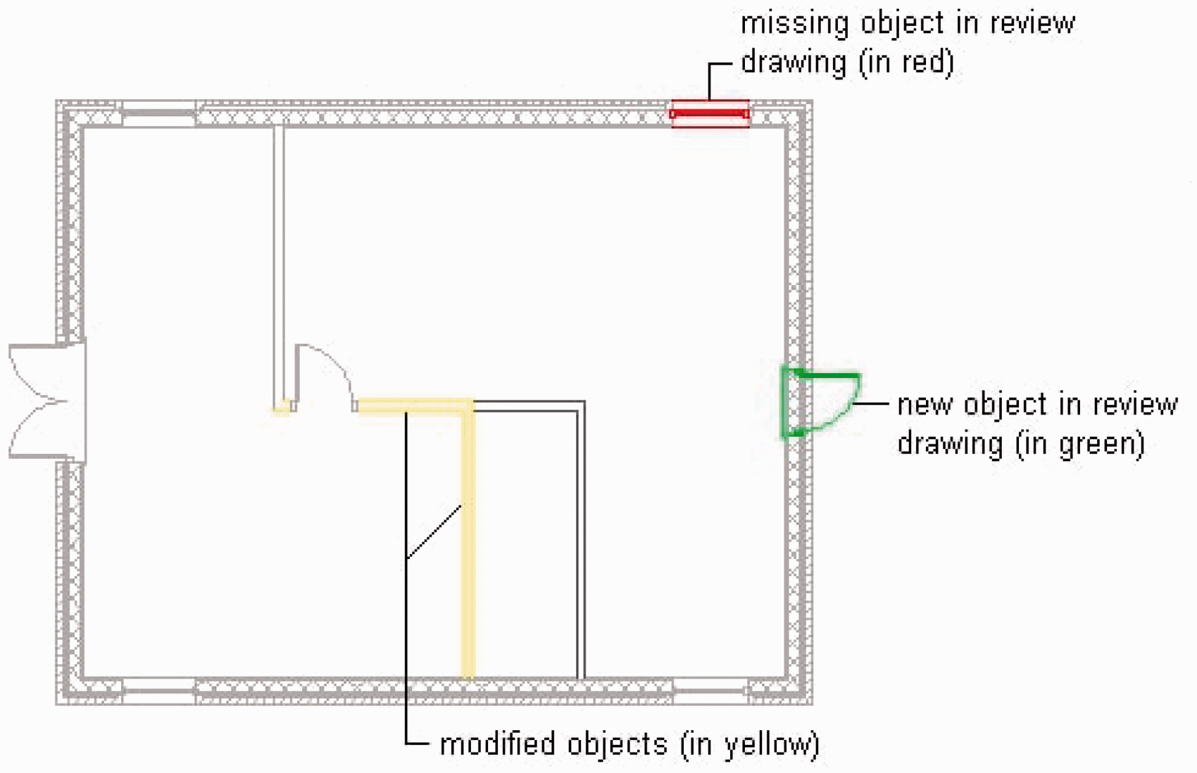
Resulting comparison.

To highlight the difference between the submission and the grading, we summarize in Table 1 other CAD tools with similar comparison features. A majority of these cannot account for differences in scale, rotations, and translations. However, PTC Creo View can be aligned by a reference point, which serves to account for some differences, but must be done manually.

Table 1.

Comparing built-in drawing comparison features of available software.

Software	SOLIDWORKS⁴	Siemens NX⁵	PTC Creo View^6,⁷	Adobe Acrobat³
Description	Compares two drawings within the Solidworks software and can overlay additions and removals in a separate file.	Compares two drawing within the NX software and overlays the drawings on top of each other.	Compares two drawings using red and green to highlight missing and additional features, respectively. Drawings can be aligned by a reference point.	Compares two PDFs pixel by pixel. Can view documents side by side, highlighting differences.
Limitations (None have inherent grading integration)	Cannot compare multiple documents simultaneously.	Cannot compare multiple documents simultaneously.	Cannot compare PDF files and can only compare one document at a time.	Cannot account for slight translations, rotations, or scaling. Can only compare one two documents at a time.
File format compatability	Compatible with CATIA, SOLIDWORKS, and Autodesk file formats.	Compatible with Autodesk, SOLIDWORKS, and NX file formats.	Compatible with Autodesk and Creo file formats.	PDF.

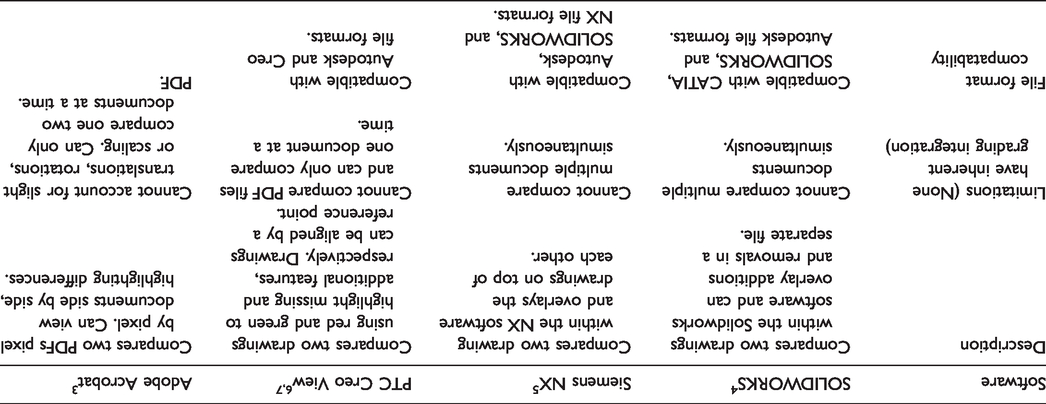
Table 1 depicts four software that have the built-in ability to compare drawing and 3 D models. Each of the software listed above simply overlays one design with a second reference design and determines what the differences are. In the case of Adobe Acrobat, it compares the two drawings pixel by pixel, which must be in PDF format, and outputs a document that highlights the differences between the two documents. While commonly used for comparing drafts of a document, if can be used to compare a student’s drawings to an assessment reference. The limitations of using Adobe Acrobat are that only one student can be compared to the reference at a time, and the software cannot account for slight variations due to rotations, translations, or differences of scale.³ SOLIDWORKS, Siemens, and PTC also offer the ability to compare both drawing and 3 D models within their software. SOLIDWORKS and NX 11 (Siemens) function similarly to Adobe in that they compare two drawings and highlight the differences, albeit on one combined sheet to better see the differences. Similarly, each can import files from other software, which allows to better account for formatting issues. However, like Adobe Acrobat, they can only compare one document at a time and cannot account for differences of rotation, translation or scale.^4,5 Lastly, PTC Creo View compares drawings, highlighting a combined drawing much like SOLIDWORKS with additional and missing feature. What sets PTC Creo View apart is that, within the software, files can be altered to set a common reference point, accounting for differences in rotation and translation. However, this software is more limited in the fie types that it can accommodate.^6,7 While a plethora of CAD software contain the architecture to compare drawings, such as those needed for grading, none of these programs have an automated way to grade multiple students, an inherent way to account for differences in scale, or a method to integrate a rubric.

Among the most limited of the graded tools created by researchers and faculty to grade student multi-view engineering drawings, Di Beneditto and Webster’s CADcompare “functions similarly to a majority of the tools listed above. It breaks down the drawing into pixels at 300 dpi and overlays the differences on top of the original student version. The software then compare every drawing within a ZIP file to the reference document, creating a new folder with the overlap and results.⁸ However, this method is limited in a variety of ways. CADcompare” cannot account for differences in translation, rotations, or scale, much like the features integrated into the various CAD tools. The software also has no method by which to grade the student’s work, as it only highlight differences between the two drawings. As this work can only compare PDF files, it offers a potential solution to students utilizing multiple CAD tools, but any formatting differences across the systems would have to be accounted for, which is not possible in it’s current state.

Kwon and McMains developed an automatic grading system for multi-view engineering drawings. They built the application using the random sample consensus (RANSAC) algorithm, estimating the affine transformations between the two individual drawings.⁹ RANSAC is an algorithm used to estimate parameters of a mathematical model from a set of data containing outliers.¹⁰ In their work, the submitted file is compared to the solution file by performing various two-dimensional operations on the submitted drawings. These transformations include projecting the drawing on the x-y plane, scaling, and/or rotating the drawing. The transformations are performed until the given drawing matches the source drawing. These transformations are then highlighted using different colors. Students’ DWG or DXF drawing files from AutoCAD are uploaded into the software using Matlab and are compared to the solution’s drawing file. An example of the Kwon’s and McMains’ work is shown in Figure 3. Note that this software is only compatible with AutoCAD-generated files and only works for 3 D drawing having three views which are front, top, and right. Furthermore, it can only detect some translation, scale, and offset errors when they are consistent in all views. Other flaws of the software include: the long duration taken by RANSAC to compare every drawing to the original, especially when there are many mistakes in the drawing to be graded; the software not providing a concrete grade; the accuracy of the software is not provided since it is only tested with two examples; and the fact that the software considers a slight error to have the same effect on the grade as a major one, e.g., a line that is slightly shifted from where it should be – could be due to RANSAC processing performed by the algorithm itself – would result in double the amount of errors than if the line did not exist at all (i.e., incorrect errors plus missing errors, instead of just a “slightly maybe incorrect” error).

Figure 3.

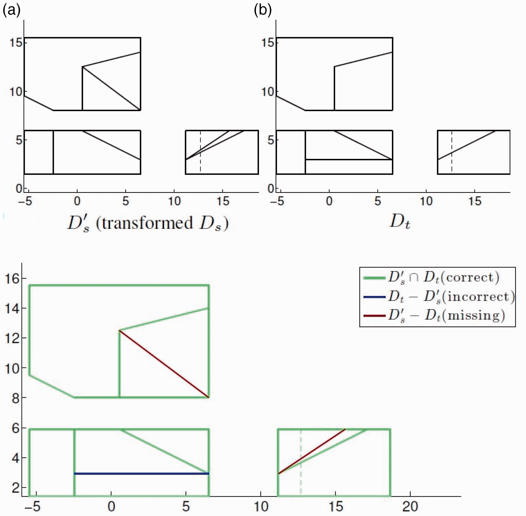
An example of Kwon’s and McMains’ algorithm in action. The two compared drawings are shown on top and the result is shown in the bottom.⁹

One of the basic approaches for developing an automated drawing grading software has been converting the drawing into a code and comparing the code parameters to calculate the differences and errors. Goh, Shukri, and Manao used that approach to propose a grading software.¹¹ The software converts the DXF files into Scalable Vector Graphics (SVG) format. The software then applies the developed marking algorithm to the SVG format and evaluates the score. However, their software only showed to perform well on a circle while not showing any information about its accuracy. It is also not fully automated, which makes it impractical to use for grading students’ drawings. Additionally, the software does not provide a concrete grade and does not correlate differences in the drawings to certain grading rubrics.

Similar work has been realized by Shukur et al, developing a software that compares DXF files from AutoCAD 2000 and grades them automatically.¹² For AutoCAD, the DXF files are in the ASCII format, which simplifies the extraction of the geometric and object parameters from the files. Hekman and Gordon used same approach and developed a software to extract geometric objects from students’ AutoCAD DWG files, compare them to a master file, and send the feedback to the student.¹³ Bryan’s software, designed for AutoCAD, used an approach similar to that of Hekman and Gordon. By extracting information of geometric objects from a DXF file in the ASCII format, the software could be compared to a master file, and give formative feedback to students. However, a glaring weakness of this approach is that all drawings must have the same reference point, as it cannot account for differences of rotation, translation, or scale. This results in one small error leading to systematic differences in the two drawings, and significantly lower grade than a human grader might give.¹⁴ San Diego University has developed a proprietary web-based application for automatic grading of drawings for Civil Engineering students.^15,16 They used group codes from the DXF files in AutoCAD to compare the technical drawings. All the above tools suffer from similar shortcomings to the ones mentioned earlier. In addition to these shortcoming, most existing work in automatic grading of 2 D drawings has been concentrated on a particular CAD software and file format.

In this work, we create an automatic grading tool, ViTA, which can also act as a pedagogical tool to enhance the learners’ experience in improving spatial visualization skills by providing immediate feedback to the student. ViTA is independent of the CAD tool used to create the drawings. It gives the user the freedom to use a CAD software of their choice; one that they are already familiar with. For example, if a student has Inventor installed on their system, they can use Inventor to create their CAD drawings; while if another is more familiar with CATIA and only has access to it, they can use CATIA to create their drawings. ViTA can then grade both drawings of this example even though they are created using two different software which might be even different from the one the instructor uses.

Virtual teaching assistant

To help teachers save time grading CAD drawings, ViTA accepts exported images of a wide range of standard formats – JPG, PNG, BMP, etc. – for the 2 D drawings from any CAD tool. The images go through a series of pre-processing steps before the drawings are analyzed and useful data is extracted. The main pre-processing steps consist of the following three steps:

Background/foreground normalization

Skeletonization

Image targeting

After pre-processing the images, several techniques are introduced to extract useful data that helps comparing two drawings and enables the detection of the following scenarios:

The two drawings are the same

The two drawings have different scales

The two drawings have different rotations/angles

The two drawings have one or more differences in hatching

The two drawings have one or more differences in the outline

The two drawings have one or more differences in line thicknesses

The two drawings have one or more differences in their structural features

The two drawings are different views of the same 3D object

The two drawings have one or more differences in terms of colors

The above steps and techniques are discussed in detail in the following sections.

Background/foreground normalization

The first step that is realized before processing any image is to have one background color and one foreground color for all images. This step enables processing all images in the same manner, no matter which CAD tool they originate from and how they are exported.

Images are first converted to black and white. Then, the background color is detected. The background color corresponds to the majority color of the pixels. If the background color is found to be black, we proceed to the next step. If the background color is found to be white, the colors of the image are inverted so that the background is always black and the foreground is always white before proceeding to the following steps.

Skeletonization

In order to have uniform line thicknesses throughout the drawings, regardless of the scale and resolution of the image, the drawings in the image are skeletonized. Skeletonization is the process of transforming all lines into one-pixel-wide lines. Many skeletonization algorithm exist and each has its own characteristics and purposes. The skeletonization algorithm used for this work is the Iterative Thinning Algorithm by Haralick and Shapiro.¹⁷

Figure 4 shows the skeletonization operation on a sample drawing.

Figure 4.

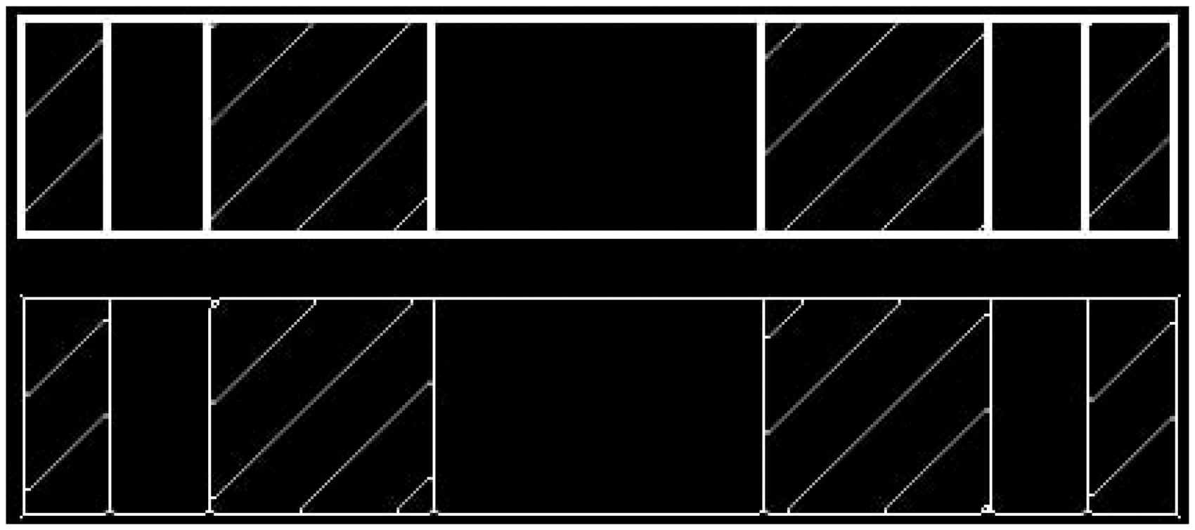
An example showing the skeletonization operation. The bottom drawing in the figure corresponds to the skeletonized image of the top drawing.

Image targeting

After the image data is skeletonized, it is time to crop the image for it to only contain the drawing of interest. This step is realized because later processing analyzes the data of the whole image. For this analysis to be correct and uniform across drawings, it is required to target the image and crop it so that it only contains the drawing of interest. The cropping is realized after finding the columns and rows with the first and last foreground (white) pixel and only keeping what is inside the obtained bounding box.

Figure 5 shows the targeting operation on a sample drawing.

Figure 5.

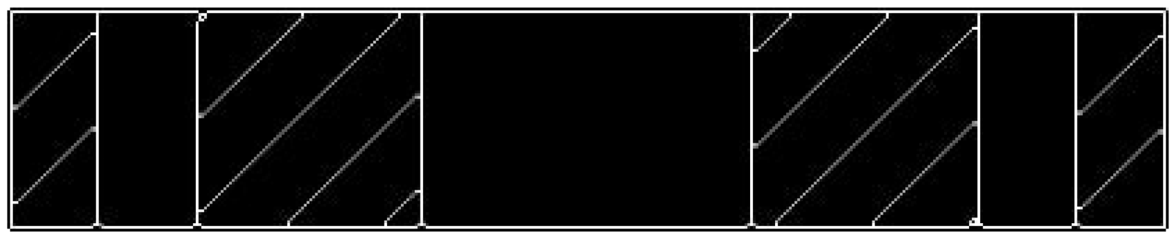
An example drawing after being cropped/targeted.

Hatching recognition

Accurately recognizing the hatching lines and hatching areas enables ViTA to recognize:

the drawings that correctly match,

and the drawings that match with respect to the structural features but contain differences in their hatching.

The following discusses these two features in detail.

Recognizing correct matches

The main feature of ViTA that could save instructors the most significant amount of time while grading CAD drawings is the ability to tell whether or not a drawing is totally correct (i.e., a given student drawing matches the correct drawing without having any mistakes). In the simple case where all drawings are known to originate from the same CAD tool with specified export settings, a simple subtraction operation between the two images to be compared could tell us whether or not they perfectly match – i.e., if the sum of pixel values in the resulting difference image is zero then there is a match, otherwise there is a mistake. In the case where there is not a preset CAD tool to use with specific preset settings, things get a little more complicated. Since hatching patterns on the drawing could be different when the drawings are built using different CAD tools or settings (see Figure 6), the hatching lines need to be first detected and then removed before comparing the drawings.

Figure 6.

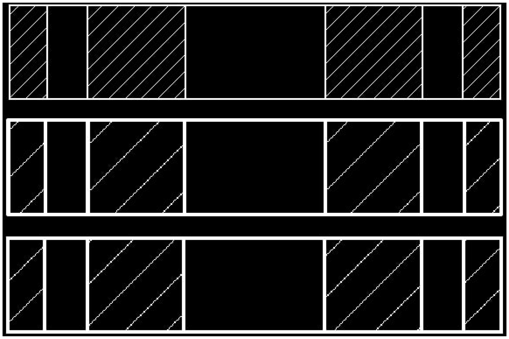
An example showing three different hatching patterns for the same drawing, each originating from a different CAD software.

In order to recognize hatching lines, Hough transform is used to detect the pixels in the skeletonized images that form 45-degree lines.¹⁸ Several Hough transform parameters need to be tuned so that it only detects hatching lines. Among these parameters, we mention the following important ones:

The tolerance/resolution – this need to be kept at a low value since all hatching lines are lines of exactly 45 degrees.

The minimum length of a line – after testing with different values, it was concluded that a good value for this is 7. This would guarantee that all the significant hatching lines are detected while no hatching lines are detected on the perimeter of a circle or curve (a curve is a sequence of pixels where some of them might form a 45-degree angle when only looking at a few consecutive pixels on the curve).

Figure 7 shows how hatching lines are detected using Hough transforms.

Figure 7.

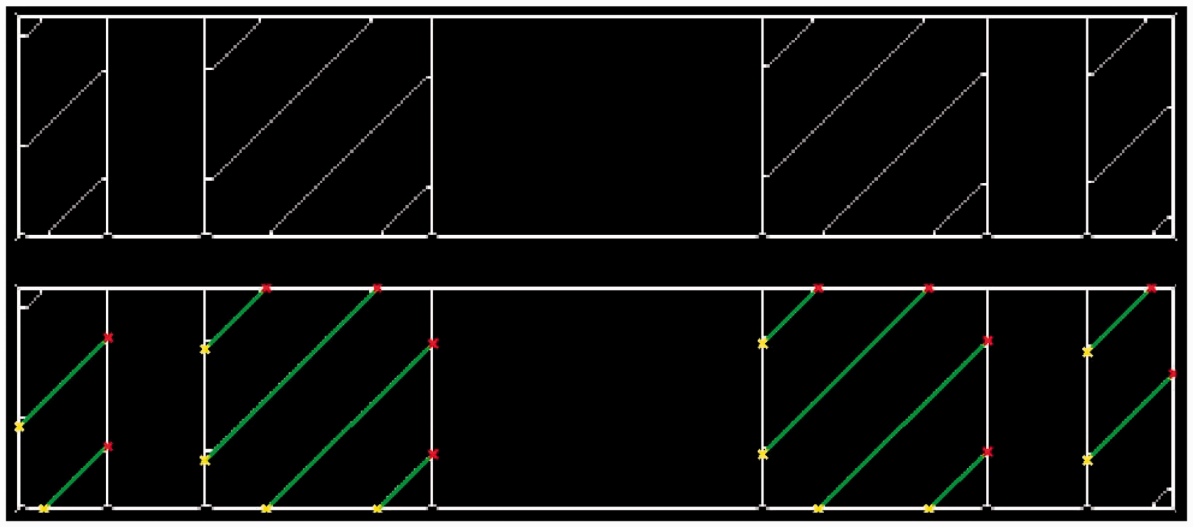
An example showing the detection of the hatching lines. The top figure shows the original image while the bottom figure shows the same image with the detected hatching lines. The ‘x’-marks show the beginning and the end of each detected hatch line.

After hatching line are detected, information about their location is stored for later analysis and then they are removed from the drawing (i.e., all their pixels are assigned the color of the background). Afterward, the images to be compared are resized to have the same dimensions. The drawings are now ready to be fairly compared while only taking their structural features into account.

To compare the drawings, at this stage, a feature vector is extracted from each drawing using a histogram of oriented gradients (HOG) feature descriptor.¹⁹ The number of HOG features – and thus the size of the feature vector – is made constant by always scaling the features’ areas’ sizes by the image size (see Figure 8 for a HOG feature extraction example). This enables the recognition of a correct drawing even if it has a mistake in scale (see the Line Thickness, Colors, and Views Section for details about scale mistakes detection). After the extraction of the HOG feature vectors from both images, the two vectors representing the images are compared. The Euclidean distance between the two vectors is computed. If this distance falls below a certain threshold, then the two images match and the given drawing is correct. Otherwise, having a distance above the threshold means that the given drawing has mistakes in its structural features.

Figure 8.

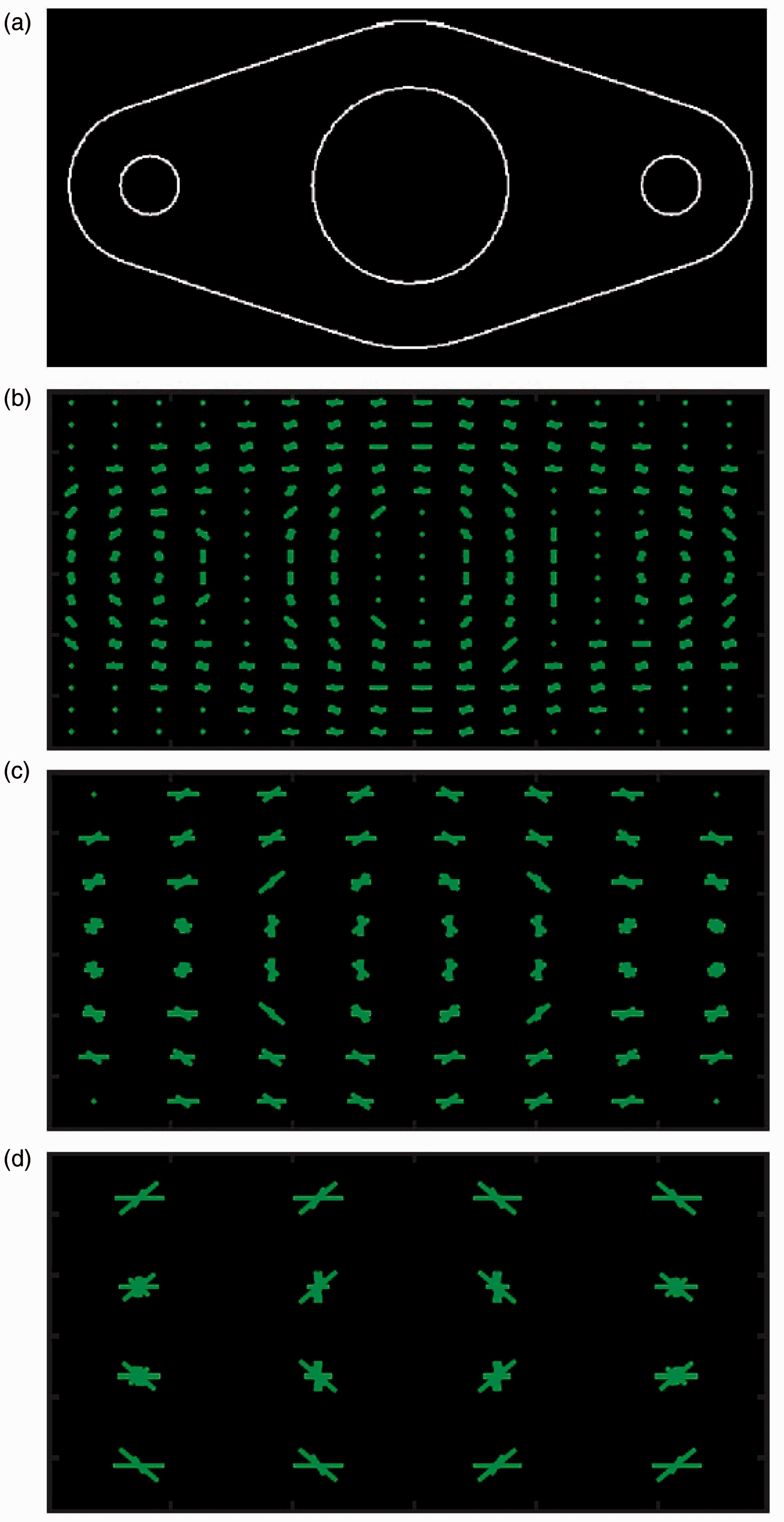
An example of the HOG feature extraction while considering different patch sizes. (a) shows the original drawing with its hatching removed. The remaining plots show the HOG features extracted with patch sizes of the original image’s dimensions divided by (b) 16, (c) 8, and (d) 4. The total size of the feature vector is 8100 features in (b), 1764 in (c), and 324 in (d).

To obtain a good threshold value that would work for the widest number and variety of drawings, we use half of the dataset of the Dataset Section having pairs of drawings that match and others that do not match (having at least one mistake/difference). This dataset was selected randomly from students’ submissions. The values of the differences between the pairs of feature vectors are analyzed using different options for the number of patches that HOG uses. It was found that dividing the image into 16x16 patches for HOG gives the best separation between the matching and the non-matching drawings, while yielding very low difference costs for the matching pairs. Therefore, the threshold was chosen to be slightly above that latter cost.

Detecting hatching mistakes

One of the ViTA’s features is the ability to compare hatching areas between two drawings in order to be able to tell whether or not these areas match. This requires the drawing to have passed the test of the Recognizing Correct Matches Section so that the structural features of the drawings match.

In the simple case where all drawings are known to originate from the same CAD tool with specified export settings, a simple comparison to know whether or not all hatching lines match in both images could tell whether or not the hatching matches. In the case where there is not a preset CAD tool to use with specified preset settings, the hatching areas are extracted by applying the following steps, illustrated in Figure 9:

Figure 9.

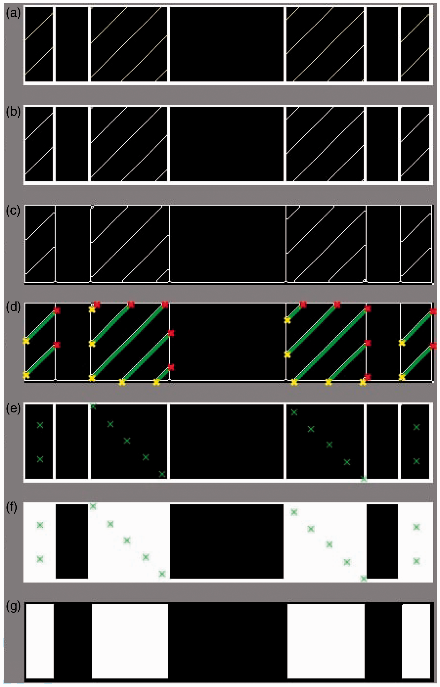
An example showing all the steps leading to the extraction of the hatching areas. (a) shows the original image. (b) shows the image converted to black and white. (c) shows the skeletonized image. (d) shows the recognized hatching lines (bold lines delimited by ‘x’ marks). (e) shows the plot of the midpoints of the hatching lines on the image after the hatching lines are removed (the midpoints are actually white pixels but they are represented by an ‘x’ mark on the figure for clarity). (f) shows the expansion of the midpoints of the hatching lines while showing where the original midpoints were (‘x’ marks). (g) shows the subtraction of (e) from (g) to obtain the resulting hatching areas.

The midpoints of all the hatching lines recognized in the Recognizing Correct Matches Section are drawn in foreground color in the image with the hatching lines removed (see Figure 9(e)).

Starting from these midpoints, the foreground color is expanded in all directions until it reaches another foreground-colored pixel. This results in all the hatching areas having the foreground color in addition to other borders (see Figure 9(f)).

The image as it was prior to Step 1 is subtracted from the resulting image of Step 2, thus leaving only the hatching areas in foreground color (see Figure 9(g)).

To detect whether or not the hatching areas match in two drawings, the resulting images of their hatching areas are compared using the same HOG features and threshold extraction technique used in the Recognizing Correct Matches Section.

A note about hatching recognition

To avoid detecting 45-degree lines that are not hatching lines, the lengths of the detected 45-degree lines in each area are examined. If a line in one hatching area is much longer than the rest of the lines in that same hatching area (i.e., the minimum difference in length between this line and all other detected hatching lines in the hatching area is significantly larger than the maximum difference in length among the other detected hatching lines), then this line would no longer be considered a hatching line. On top of that, a minimum number of two hatching lines that are longer than the minimum required length is needed in a hatching area for the lines to be considered hatching lines.

Note that such cases rarely occur, and even if a 45-degree line is mislabeled (i.e., a hatching line v. not a hatching line), it would be mislabeled in both drawings that are being compared – if they match – and would still lead to a correct scoring of the drawing.

Outline detection

Another feature of ViTA is the ability to detect whether or not the outlines of two drawings match. This could let graders give some points to the student in case they have mistakes in some structural features but the outline of the drawing is correct. We mean by “outline” the outside contour of the drawing, disregarding the details that might be inside that contour.

To detect the outline, each pixel having the background color is traversed and exploded. The explosion of the pixel makes it take the foreground color and infects its four connected neighboring pixels, which, in turn, propagate this explosion. The explosion stops when the wave of infected pixels reaches other foreground-colored pixels or the edges of the image. If a whole explosion is confined within foreground-pixel boundaries, the explosion is kept; otherwise, it is undone. Figure 10 shows an example of the outline detection.

Figure 10.

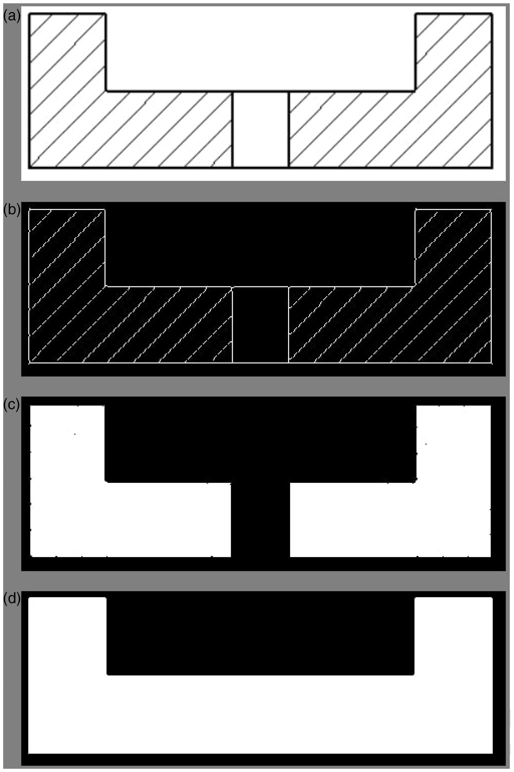
An example showing the outline detection. (a) shows the original image. (b) shows the skeletonized image after the background is normalized to be black. (c) shows the detected hatching areas to show the difference between them and the outline image. (d) shows the obtained outline image.

After the outline image is obtained from both drawings to be compared, the same HOG feature extraction and thresholding technique of the Hatching Recognition Section is used to decide whether or not it is a match. In the simpler case where all drawings are known to originate from the same CAD tool with specified export settings, image subtraction could be used to determine whether or not the outlines match, as described in the Hatching Recognition Section.

Scale and orientation

On top of the previously discussed features, ViTA can also detect mistakes is scale and in orientation.

The mistakes in scale are simply detected when the two drawings have different sizes but they end up passing all the previous tests and scoring correctly.

The mistakes in orientation are detected by first rotating the drawing to be graded by a small increment and cropping it (targeting) until its aspect ratio matches the one of the drawing to compare to. If the drawing goes through 360 degrees of rotation without a match in aspect ratio, then the drawing is incorrect – i.e., has mistakes in its structural features. If there is a match in the aspect ratio, tests of the Hatching Recognition Section – and of the Outline Detection Section, if required – are conducted to test for a match. If there is a match, then the only mistake would be in the orientation (unless there is an additional scaling mistake). If the tests for a match (or match in outline) fail, one last test for a match is conducted after rotating the image by another 180 degrees (still, same aspect ratio). If the latter test fails, then the drawing is incorrect – i.e., has mistakes in its structural features. Note that, when rotating an image, the image is always expanded to accommodate the existing parts of the drawing; the newly created areas of the image are filled with the background color.

Line thickness, colors, and views

Even though these types of mistakes are not always applicable to the drawings, we added to ViTA’s platform the capability to detect if two images are identical but differ in line thickness, if they are different in terms of colors, and if they are two views of the same 3 D object.

To detect differences in line thickness between the two images, after passing the correctness test mentioned previously, we simply retest while skipping skeletonization. Color differences are easily detected by retesting while skipping conversing to black and white and comparing pixel values. We even included an option to use the Hue value of the HSV color space instead of red, green, and blue values of the RGB color space, which enables us to be less strict with different shades of the same color. As for detecting that an image is a different (incorrect) view of the same 3 D object, we simply include the correct images of those different views and compare to them as well.

Evaluation

In this section, we discuss the evaluation of ViTA and present the obtained results.

Grading rubric

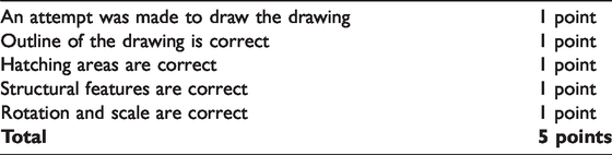
ViTA is a toolbox that can recognize matching and non-matching drawings while offering the detection of multiple mistakes in a 2 D cross-sectional drawing, as discussed in the Virtual Teaching Assistant Section. To evaluate all the features that ViTA offers, we used a slightly modified version of the grading rubric of Ingale et al.²⁰ that is summarized in Table 2. The rubric of Ingale et al.²⁰ considers the same criteria of Table 2 except for giving a point for a correct cutting plane perspective instead of correct rotation and scale. Since the cutting plane would be correct if the rest of the criteria is correct, we decided to replace it with rotation/scale check in order to show the most out of ViTA’s capabilities. Note that ViTA’s different features could be turned on and off, as needed. ViTA’s remaining features that are not tested through this dataset were also tested with other drawings and showed success.

Table 2.

The grading rubric used for evaluation.

An attempt was made to draw the drawing	1 point
Outline of the drawing is correct	1 point
Hatching areas are correct	1 point
Structural features are correct	1 point
Rotation and scale are correct	1 point
Total	5 points

Graphical user interface

To present ViTA in a user-friendly manner that can be used across different CAD software and useful to the grader, we created a standalone graphical user interface (GUI) that contains two modes:

1. Grading one file at a time (see Figure 11).

Figure 11.

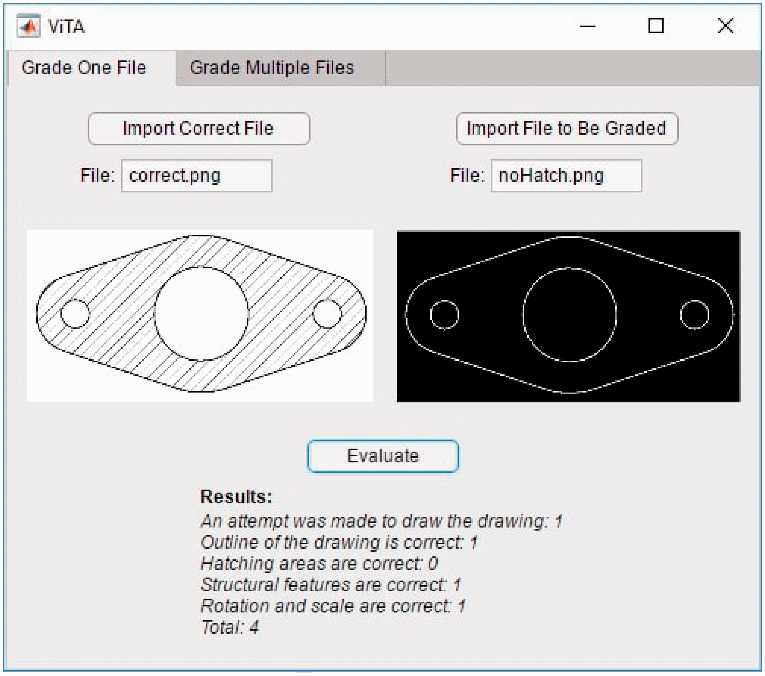
An example showing ViTA’s GUI while grading one drawing. The user presses on the “Import Correct File” button to import the correct baseline file and on the” Import File to Be Graded” button to import the file that they desire to grade. The names of the chosen files are shown respectively under each button and their images are shown below them. After both files are imported, the user presses the “Evaluate” button for the grading to happen and the results to be shown.

2. Grading multiple files (see Figure 12).

Figure 12.

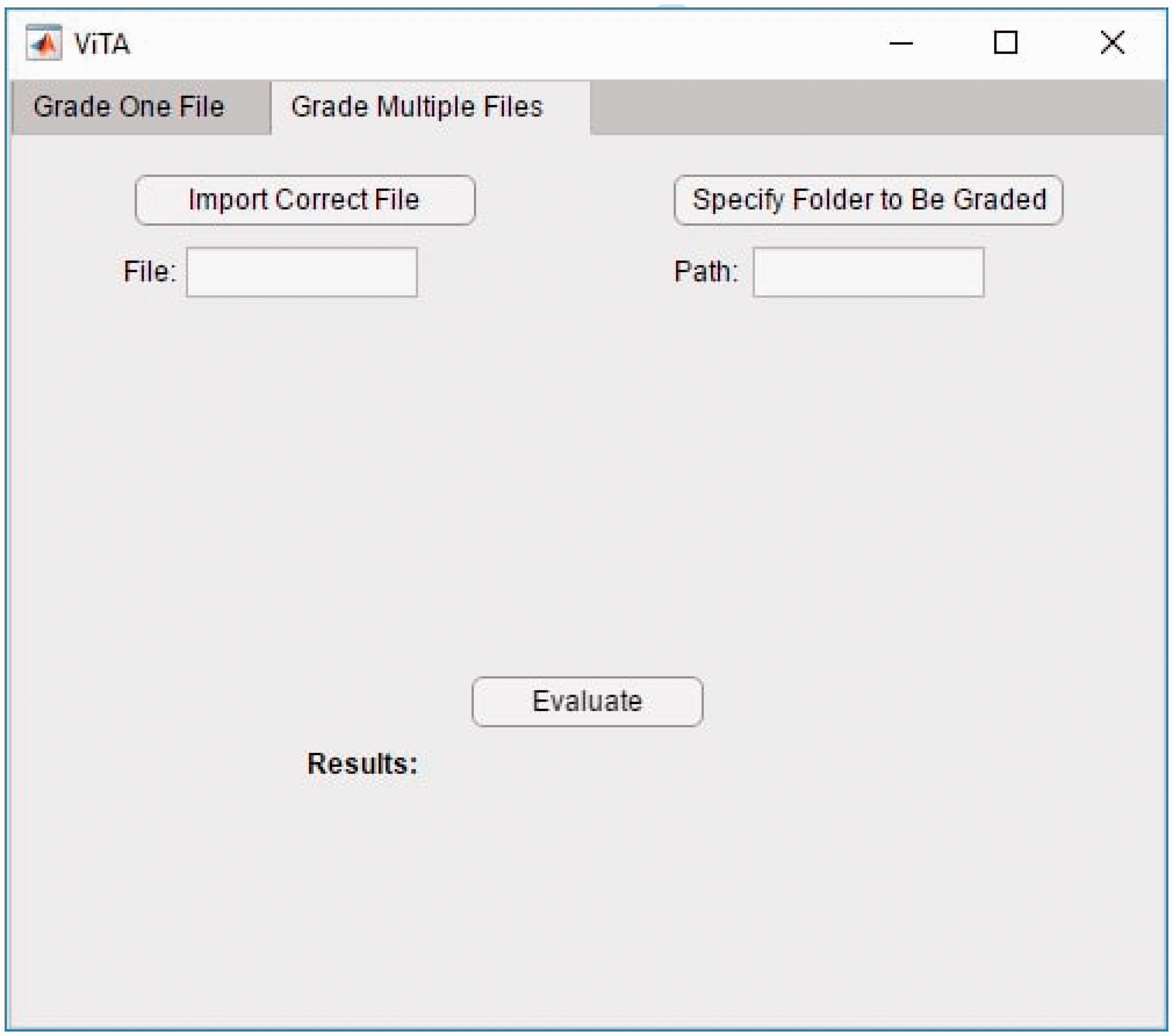
ViTA’s GUI for the option of grading multiple drawings. The user presses on the “Import Correct File” button to import the correct baseline file and on the “Specify Folder to Be Graded” button to specify the directory holding all the files to be graded. The names of the correct file and the directory are shown respectively under each button and the image of the correct file is shown below them in the center. After both files are imported, the user presses the “Evaluate” button for the grading to happen and the results to be shown. Note that, in this case, each file’s name is shown before its results are listed and a vertical scrolling bar appears to help the user navigate through the results.

The first mode is used when there is a need to grade one drawing by comparing it to the correct drawing. The second mode is used when there is a need to grade multiple files of the same drawing – e.g., when grading an assignment given to a whole class or group of students. In both modes, the results show the detailed grading of each file along with the total points for that file, as shown in Figure 11.

Dataset

The dataset used to evaluate ViTA consists of 500 CAD submissions collected in an undergraduate Introduction to Spatial Visualization course at Virginia Tech. These submissions included CAD sectional drawings for mechanical structures (see Figure 13) originating from three different CAD tools (Inventor,²¹ CATIA,²² and SOLIDWORKS²³). The CAD drawings are first exported to images and labeled according to whether they are correct or contain mistakes, while specifying the types of these mistakes. The mistakes that existed in the dataset were sometimes a combination of more than one type of mistake.

Figure 13.

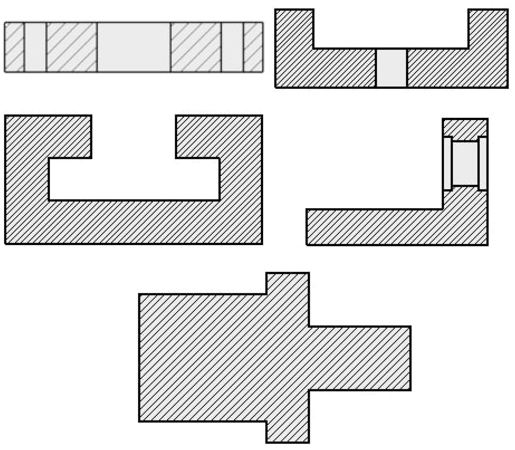
Some of the drawing types used to evaluate ViTA. Others are shown in the previous Figures.

Results and discussion

Using the second half of the dataset of the Dataset Section that is not used in the training realized in the Recognizing Correct Matches Section, ViTA was evaluated by feeding it a sample of a correct drawing and other samples that might be correct or containing mistakes.

The results were compared to the ground truth and showed that ViTA was successfully able to correctly grade all – i.e., 100% of – the drawings. It was able to correctly identify all correct drawings, all the mistakes in the drawings, and give them appropriate grades. The only observed catch was that, when having a totally incorrect drawing, ViTA takes some time to test for a rotation mistake (i.e., rotating the image by a small increment and checking, then keep repeating until the image is fully rotated). The same issue occurs when there is actually a rotation mistake, but the rotations would stop when the mistake is detected. This time-related issue does not impact small and relatively simple drawings because the increments of rotation could be set to much higher than the ones that should exist for more complicated/detailed drawings. For more complicated drawings, one could raise the matching thresholds and use lower increment values, but this could potentially lead to having some false positives (i.e., slightly incorrect drawings classified as being correct). The latter case is not advised since the main goal of ViTA is to save time for the grader. This means that a grader would normally prefer to trust the software to correctly recognize all correct drawings so that they do not have to waste time double checking; that would defy the purpose of the software. In case the grader has a lot of files to grade and the software is taking some time to grade them, it would usually still be much faster than a human correcting them. If the rubric is set to not include rotation mistakes, ViTA would always finish in a short amount of time. In our evaluation, it took ViTA less than a minute to grade all 500 submissions, compared to about six hours when graded by a TA. More realistically, using traditional grading, students got feedback from the instructor/TA about one week after submitting their drawing. Therefore, ViTA saves significant time for the graders and helps students learn much faster from their mistakes.

One limitation to the conducted evaluation was the limited difficulty and details in drawings that were evaluated (those were the only types of drawings used in the course). Even though we tested a large number of drawings with different types of mistakes, there might exist some cases in future drawings where the drawings that come from different CAD tools contain a lot of detail with one minor mistake. Compared to the amount of detail that matches in the drawing, that mistake might be undetected, depending on its type. To avoid this issue, threshold must be set to stricter values, if not even zero. This would lead to always having the drawings classified as “correct” to be correct ones, while some correct ones might end up being classified as having mistakes in their features, then the grader would just double-check those incorrect ones. Note that this issue would rarely occur in very specific cases where the following constraints are met:

The two drawings originate from different CAD tools.

The export settings in the different CAD tools are different.

The drawings have a large size.

The drawings contain a lot of detail.

There is a very minor mistake in a drawing.

Future work will concentrate on testing such cases with real and synthetic data while exploring different ways to solve such issues, such as having a dynamic HOG patch size and training using a significantly larger amount of data with many more shapes.

Conclusion and future work

This work introduces a new tool that helps instructors save time when grading CAD drawings. This tool, called ViTA, offers the ability to compare two-dimensional drawings originating from different CAD tools and grades them automatically according to a flexible grading rubric that the human grader sets. ViTA has the ability to recognize correct drawings and can detect multiple popular mistakes that the instructor would look for, such as mistakes in structural features, outline, hatching, orientation, scale, line thickness, colors, and views. Evaluating ViTA using a relevant grading rubric showed its accuracy, speed, and relevance in automatically grading two-dimensional drawings.

Future work will focus on testing ViTA with more complex drawings and with synthetic shapes that slightly vary from the correct drawing. This will involve upgrading ViTA to use smarter algorithms that might involve machine learning and deep learning. We will also concentrate on expanding ViTA to include the automatic grading of three-dimensional drawings and the ability to automatically extract the drawings’ images from their corresponding CAD files.

Footnotes

Acknowledgements

We would like to thank Mr. Sanchit Ingale who helped with the conversion of CAD files to images used in our experiments.

Declaration of conflicting interests

The author(s) declared no potential conflicts of interest with respect to the research, authorship, and/or publication of this article.

Funding

The author(s) received no financial support for the research, authorship, and/or publication of this article.

ORCID iD

Rabih Younes

References

AUTODESK Help. About drawing compare, https://knowledge.autodesk.com/support/autocadarchitecture/learn-explore/caas/CloudHelp/cloudhelp/2018/ENU/AutoCAD-Architecture/files/GUID-20918F56-EDE6-42B6-AE13-E06CB0C66D37-htm.html (2019, accessed 7 July 2020).

Guerci

Baxter

DH.

Automating an introductory computer aided design course to improve student evaluation. In: ASEE annual conference proceedings, Nashville, TN, 2003, pp. 6503–6510.

Acrobat

Compare two versions of a PDF File (Acrobat Pro), https://helpx.adobe.com/acrobat/using/compare-documents.html (2020, accessed 7 July 2020).

Dassault Systemes. Running the Compare Utility, https://help.solidworks.com/2017/English/SolidWorks/swutilities t. _running. _the. _compare. _utility.htm. (2017, accessed 7 July 2020).

Siemens. Compare Drawing Revisions Pt. 1: Track Drawing Changes in NX 11, https://community.sw.siemens.com/s/article/compare-drawing-revisions-pt-1-track-drawing-changes-in-nx-11. (accessed 7 July 2020).

Ramesh

Comparing Drawings, Models, and PCBs with PTC Creo View, www.ptc.com/en/cad-software-blog/comparing-drawings-models-and-pcbs-with-ptc-creo-view (2014, accessed 7 July 2020).

PTC. Feature Comparison of PTC Creo View MCAD Product Suite, www.econocap.com/wp-content/uploads/2018/01/View_MCAD_Product_Suite.pdf (2013, accessed 7 July 2020).

Di Beneditto

Webster

CADcompareTM: a web-based application that compares PDF CAD drawings. In: ASEE annual conference and exposition, conference proceedings, 24-27 June, 2018.

Kwon

McMains

An automated grading/feedback system for 3-view engineering drawings using Ransac. In: Proceedings of the Second (2015) acm conference on learning @ Scale, L@S 15. New York: ACM, 2015, pp. 157–166.

10.

Fischler

Bolles

RC.

Random sample consensus: a paradigm for model fitting with applications to image analysis and automated cartography. Commun Acm 1981; 24: 381–395.

11.

Goh

Mohd Shukri

Manao

Automatic assessment for engineering drawing. In: Zaman

Robinson

Olivier

, et al. (eds) Advances in visual informatics. Cham: Springer International Publishing, 2013, pp. 497–507.

12.

Shukur

Away

Dawari

MA.

Computer-aided marking system for engineering drawing. In: Ferdig

, Crawford

Carlsen

, et al. (eds) Proceedings of society for information technology & teacher education international conference. Atlanta, GA: Association for the Advancement of Computing in Education (AACE), 2004, pp.1852–1857.

13.

Hekman

Gordon

MT.

Automated grading of first year student cad work automated grading of first year student cad work. In: 120th ASEE Annual Conference and Exposition, 23-26 June, 2013.

14.

Bryan

JA.

Automatic grading software for 2D CAD files. Comput Appl Eng Educ 2020; 28: 51–61.

15.

Karna

Enhanced AutoCAD grading application: backend component. San Diego, CA: San Diego State University, 2012.

16.

Ivaturi

Enhanced AutoCAD grading application: frontend. San Diego, CA: San Diego State University, 2012.

17.

Haralick

Shapiro

LG.

Computer and robot vision. Reading, MA: Addison-Wesley, 1993.

18.

Duda

Hart

PE.

Use of the Hough transformation to detect lines and curves in pictures. Commun Acm 1972; 15: 11–15.

19.

Dalal

Triggs

Histograms of oriented gradients for human detection. In: 2005 IEEE computer society conference on computer vision and pattern recognition (CVPR’05). vol. 1. New York: IEEE, 2005, pp. 886–893.

20.

Ingale

Srinivasan

Bairaktarova

CAD platform independent software for automatic grading of technical drawings. In: Proceedings of the ASME 2017 international design engineering technical conferences & computers and information in engineering conference (IDETC/CIE 2017). Cleveland, OH, USA, 6-9 August, 2017.

21.

AUTODESK. Inventor, www.autodesk.com/products/inventor/overview (2019, accessed 7 July 2020).

22.

3DS. CATIA 3DEXPERIENCE. https://www.3ds.com/products-services/catia/ (2019, accessed 7 July 2020).

23.

SOLIDWORKS. https://www.solidworks.com/ (2020, accessed 7 July 2020).