Instantaneous center/axis of rotation for planar and three-dimensional motion

Abstract

This article discusses a direct analytical method for calculating the instantaneous center of rotation and the instantaneous axis of rotation for the two-dimensional and three-dimensional motion, respectively, of rigid bodies. In the case of planar motion, this method produces a closed-form expression for the instantaneous center of rotation based on a single point located on the rigid body. It can also be used to derive closed-form expressions for the body and space centrodes. For three-dimensional, rigid body motion, an extension of the technique used for planar motion locates a point on the instantaneous axis of rotation, which is parallel to the body angular velocity vector. In addition, methods are demonstrated that can be used to map the body and space cones for general rigid body motion, and locate the fixed point for the body.

Keywords

Rigid body dynamics centrodes instantaneous axis of rotation

Introduction

Determination of the instantaneous center of rotation (ICR) for a rigid body in planar motion, and the associated body and space centrodes, has always provided a basis for understanding complex mechanisms in machines.¹ More recently, the field of biomedical engineering has found those concepts to be critically important for the design of prostheses.^2,3 Undergraduate dynamics textbooks^4–7 typically present two scenarios from which the ICR may be determined. In both cases, the velocities of two points on the body are given. Both cases are valuable from a pedagogical perspective since a graphical interpretation readily identifies the ICR. As presented, the location of the ICR is calculated by first expressing the velocity vectors in scalar form. Herein, these will be referred to as “indirect” methods.

A third case, where the velocity of a single point on the body and the angular velocity of the body are given, is also included in several textbooks,^4,5 and implied by others.^6,7 Calculations of the ICR location, as presented in the aforementioned textbooks and other articles,^8–11 also employ an indirect method in which the velocity and angular velocity vectors are first expressed in scalar form. While investigating the possible existence of a direct, analytical method for calculating the ICR, the author came across a post¹² in the Physics forum of StackExchange. In this discussion, a direct, analytical expression for calculating the ICR was presented. Proof was offered in a linked post,¹³ which also addressed three-dimensional motion, but no sources from refereed journals or textbooks were cited in either post. Further investigation uncovered the same closed-form expression with a brief explanation in the Dynamics course¹⁴ under Aeronautics and Astronautics offered by MIT OpenCourseWare.

For general, three-dimensional motion, Chasles’ theorem^15,16 states that general motion of a rigid body consists of the resultant of an Euler rotation and a translation parallel to the axis of rotation. The axis to which Chasles’ theorem refers is the instantaneous axis of rotation (IAR). The concept of an IAR may be considered to be an extension of an ICR, where the ICR is simply a point located somewhere along the IAR. Several undergraduate textbooks^4–6 briefly discuss IARs and the associated space and body cones, which are analogous to the space and body centrodes, but none provide detailed descriptions of how they may be calculated. Nor could the author find any explanations of exactly how one may calculate the IAR, space cone, and body cone.

In order to provide a firm foundation for the discussion of general, three-dimensional motion, this article will begin with a derivation of the direct method for calculating the ICR. In addition, a description of how the body and space centrodes may be calculated will be included. Then, a method for determining the location of the IAR, space cone, and body cone for a three-dimensional rigid body will be derived using the direct method for calculating the ICR as a starting point. Examples of how the derived methods may be applied will be provided.

Planar, rigid body kinematics

In this section, a direct, analytical method that can be used to calculate the location of the ICR for a rigid body undergoing planar motion will be presented and discussed. It should be understood that the ICR may also be interpreted as a single point on the axis about which the body rotates. For the case of planar motion, however, this article will address only the location of the ICR. Following the derivation of the analytical expression, an example will be provided to demonstrate the method.

Derivation for planar motion

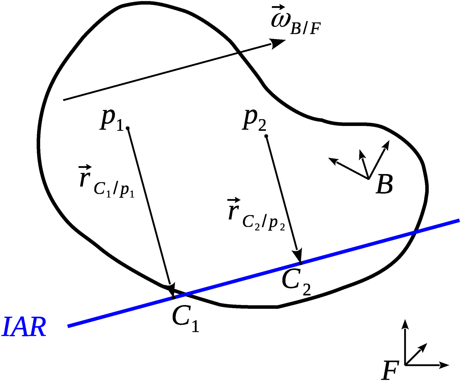
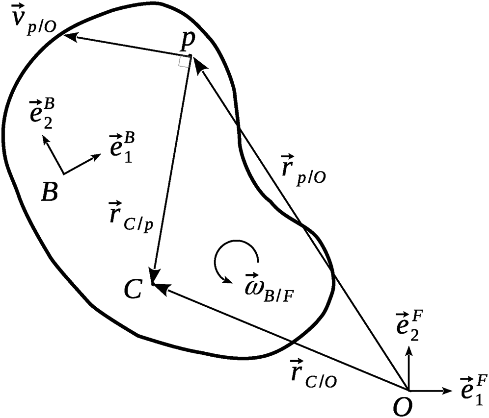
Figure 1 shows a rigid body that is translating and rotating with respect to a global reference frame $F$ . The basis vectors that define the $F$ reference frame are ${\vec{e}}_{1}^{F}$ , ${\vec{e}}_{2}^{F}$ , and ${\vec{e}}_{3}^{F}$ , where ${\vec{e}}_{3}^{F}$ is always perpendicular to the plane of motion. A local reference frame $B$ is embedded in the rigid body and is defined by the basis vectors ${\vec{e}}_{1}^{B}$ , ${\vec{e}}_{2}^{B}$ , and ${\vec{e}}_{3}^{B}$ , where ${\vec{e}}_{3}^{B}$ is also always perpendicular to the plane of motion. Point $O$ is fixed in the $F$ reference frame and, without loss of generality, may be located at the origin of $F$ . Point $p$ is a point that is fixed at any arbitrary point in the body, and $C$ is the unknown location of the ICR. By definition, the velocity of the ICR with respect to any point fixed in $F$ is equal to the null vector.

Figure 1.

Planar motion of a rigid body where $C$ is the instantaneous center of rotation (ICR) and $p$ is an arbitrary point on the body. The body is rotating with an angular velocity ${\vec{w}}_{B / F}$ .

The vector location of the ICR ( $C$ ) with respect to $O$ may be decomposed into components that go through point $p$ .

{\vec{r}}_{C / O} = {\vec{r}}_{C / p} + {\vec{r}}_{p / O}

(1)

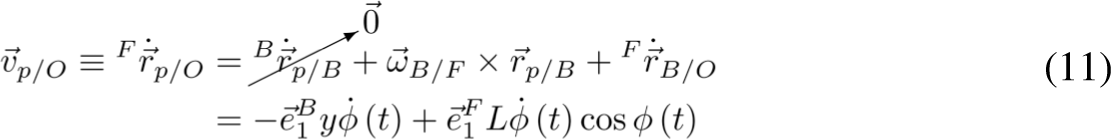
Calculate the velocity of

C

with respect to

O

by taking the time derivative in

F

of equation (1).

{\vec{v}}_{C / O} \equiv^{F} {\dot{\vec{r}}}_{C / O} =^{F} {\dot{\vec{r}}}_{C / p} +^{F} {\dot{\vec{r}}}_{p / O}

(2)

The first term on the right-hand side of equation (2) may be expanded using the transport theorem for kinematics,⁴ which uses the angular velocity of the body (

B

) with respect to the global reference frame (

F

By definition, ${\vec{v}}_{C / O}$ in equation (3) is equal to the null vector. In addition, the time derivative in $B$ of the position of $C$ with respect to $p$ is equal to the null vector because both points are fixed in $B$ .

In equation (3), ${\vec{r}}_{C / p}$ is the vector that we desire to calculate, and the other two vectors, ${\vec{v}}_{p / O}$ and ${\vec{w}}_{B / F}$ are known or can easily be calculated. In order to solve for ${\vec{r}}_{C / p}$ , we can cross ${\vec{w}}_{B / F}$ with each term in equation (3).

Apply the identity for vector triple products.

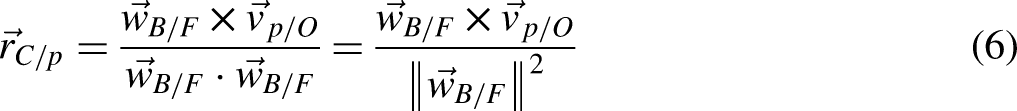
- ({\vec{w}}_{B / F} \cdot {\vec{w}}_{B / F}) {\vec{r}}_{C / p} + {\vec{w}}_{B / F} \times {\vec{v}}_{p / O} = \vec{0}

(5)

Finally, equation (5) can be solved for the position of the ICR with respect to any arbitrary point on the body.

{\vec{r}}_{C / p} = \frac{{\vec{w}}_{B / F} \times {\vec{v}}_{p / O}}{{\vec{w}}_{B / F} \cdot {\vec{w}}_{B / F}} = \frac{{\vec{w}}_{B / F} \times {\vec{v}}_{p / O}}{{‖ {\vec{w}}_{B / F} ‖}^{2}}

(6)

In and of itself, equation (6) accomplishes little more than the indirect methods described in undergraduate dynamics texts. That is, it calculates the location of the ICR for one instant in time. The utility of equation (6) is found when one wishes to calculate the body centrode (polhode curve) and space centrode (herpolhode curve) associated with the motion of the body. Using the definitions from the analysis above, the body centrode is the locus of points defined by

{\vec{r}}_{C / p}

in equation (6) for all values of the time. Similarly, the space centrode is the locus of points defined by

{\vec{r}}_{C / O}

in equation (1) for all values of the time.

{\vec{r}}_{C / O} = \frac{{\vec{w}}_{B / F} \times {\vec{v}}_{p / O}}{{‖ {\vec{w}}_{B / F} ‖}^{2}} + {\vec{r}}_{p / O}

(7)

Planar example

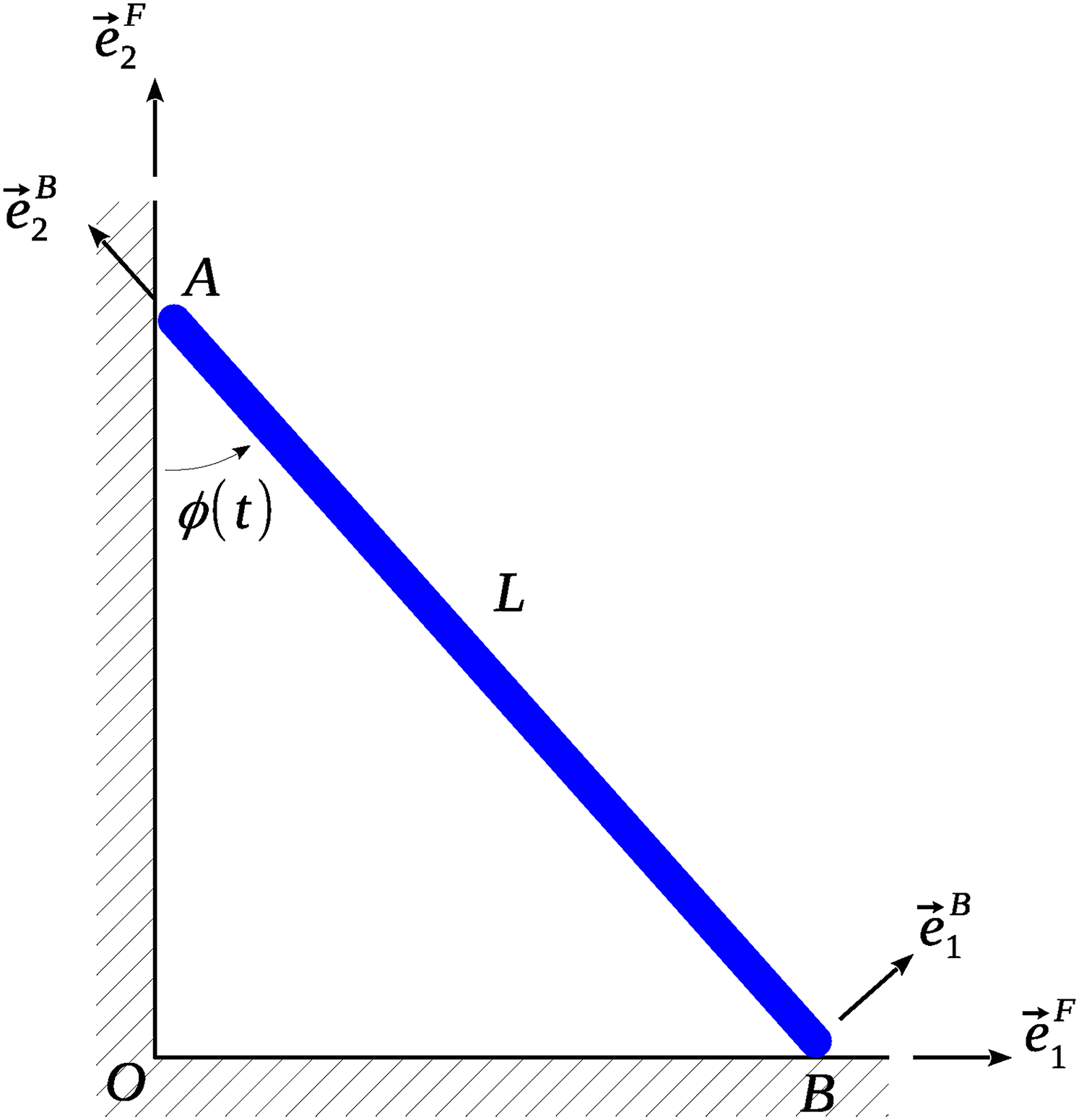
The familiar example of a ladder sliding down a wall will be used to demonstrate the utility of the method described above for calculating the ICR and the space and body centrodes. Initially, the ladder is leaning against a wall in a vertical position. It then slides down the wall and across the floor to a final horizontal position, while constantly keeping contact with both the wall and floor (see Figure 2). Reference frame $F$ is fixed to the wall/floor and frame $B$ is fixed to the ladder, which has length $L$ . The origin of $F$ is located at point $O$ , and the origin of frame $B$ is located at point $B$ which is always in contact with the floor. Point $A$ on the ladder is always in contact with the wall. Using an arbitrary position $p$ on the ladder ( ${\vec{r}}_{p / B} = y {\vec{e}}_{2}^{B}$ ), we wish to calculate the position of the ICR $C$ as a function of $ϕ (t)$ , the angle between the wall and the ladder.

Figure 2.

Planar motion of a ladder sliding down a wall. Points $A$ and $B$ are constantly in contact with the wall and floor, respectively.

First, define the location of $p$ with respect to $O$ .

{\vec{r}}_{p / O} = {\vec{r}}_{p / B} + {\vec{r}}_{B / O}

(8)

where

p

is located at an arbitrary distance

y

from

B

on the ladder, in the

{\vec{e}}_{2}^{B}

direction.

{\vec{r}}_{p / B} = {\vec{e}}_{2}^{B} y

(9)

{\vec{r}}_{B / O} = {\vec{e}}_{1}^{F} L \sin ϕ (t)

(10)

Next, calculate the velocity of $p$ with respect to $O$ using equations (8)–(10). where ${\vec{w}}_{B / F} = \dot{ϕ} (t) {\vec{e}}_{3}^{B} = \dot{ϕ} (t) {\vec{e}}_{3}^{F}$ . Finally, the position of the ICR with respect to $p$ may be calculated using equation (6).

{\vec{r}}_{C / p} = - {\vec{e}}_{2}^{B} y + {\vec{e}}_{2}^{F} L \cos ϕ (t)

(12)

There are a couple of observations relating to the solution in equation (12) that are worth noting. First, the calculation of the ICR was performed using mixed bases. In general, for planar motion only, this is easy to do because the direction of the angular velocity vector is constant. Second, the first term in equation (12) always brings the location of the ICR back to point

B

. So, by setting

y = 0

, the ICR can simply be found relative to the location of

B

Since equation (12) provides a closed-form expression for the ICR as a function of $ϕ (t)$ , it should be an easy matter to calculate and plot closed-form expressions for the space and body centrodes. The space centrode is defined as the position of $C$ with respect to $O$ in the $F$ reference frame. Taking advantage of the second observation above, it can be assumed, without loss of generality, that $y = 0$ . equations (12) and (8) may be used to calculate ${\vec{r}}_{C / O}$ .

{\vec{r}}_{C / O} = {\vec{r}}_{C / p} + {\vec{r}}_{p / O} = L [{\vec{e}}_{1}^{F} \sin ϕ (t) + {\vec{e}}_{2}^{F} \cos ϕ (t)]

(13)

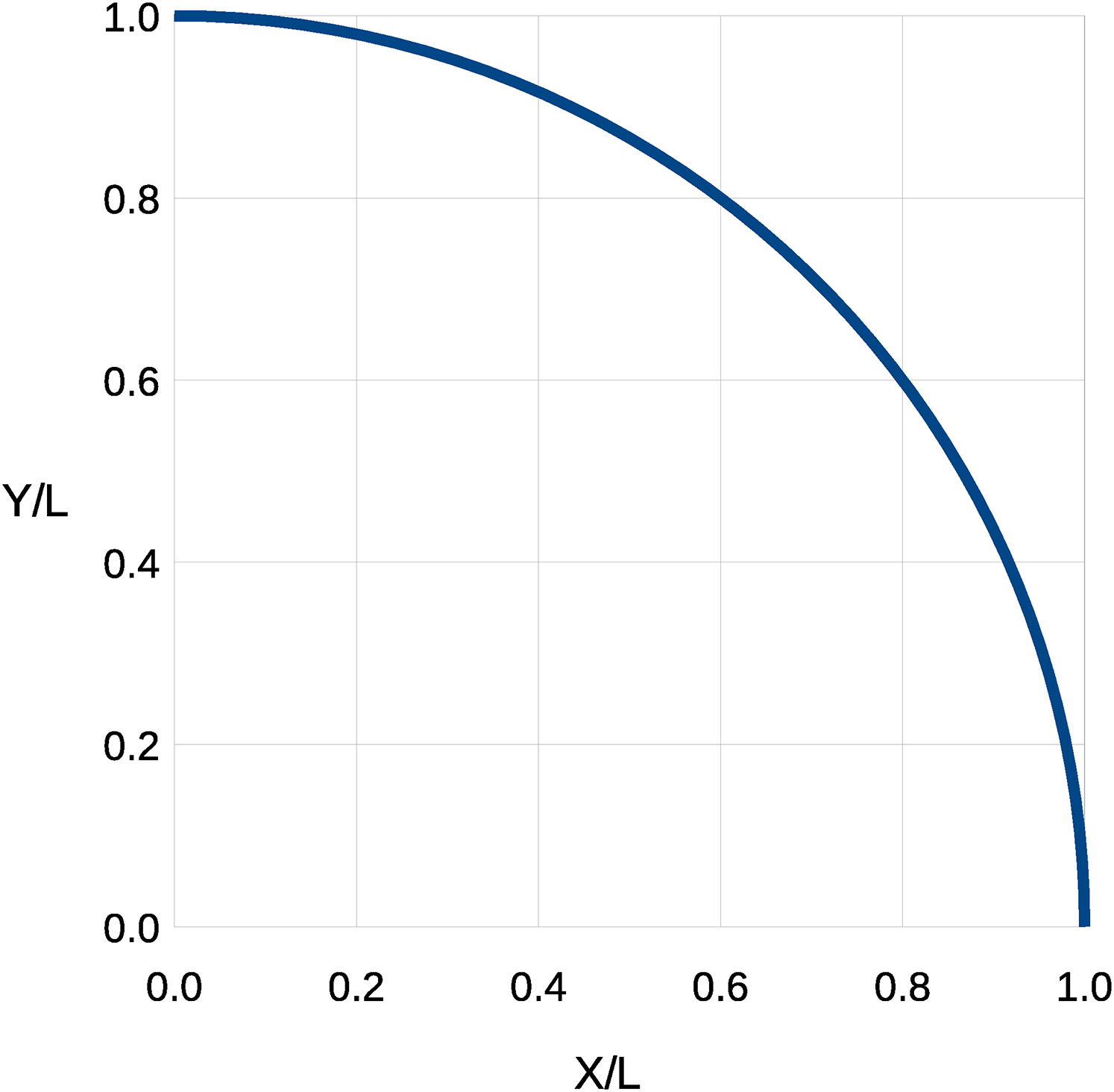
Since the inital position of the ladder is vertical and the final position is horizontal,

0^{\circ} \leq ϕ (t) \leq 90^{\circ}

. The space centrode in Figure 3 is plotted in terms of coordinates

X

and

Y

in the

{\vec{e}}_{1}^{F}

and

{\vec{e}}_{2}^{F}

directions, respectively.

Figure 3.

Space centrode in $F$ coordinates, where the left and bottom edges of the graph correspond to the wall and floor, respectively, in Figure 2.

The body centrode is defined as the position of $C$ with respect to $B$ in the $B$ reference frame, again assuming that $y = 0$ .

Transform the ${\vec{e}}_{2}^{F}$ basis vector into $B$ basis vectors using Figure 2.

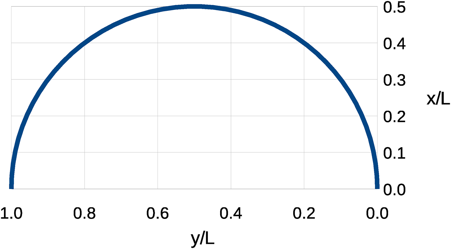
{\vec{r}}_{C / B} = L \cos ϕ (t) [{\vec{e}}_{1}^{B} \sin ϕ (t) + {\vec{e}}_{2}^{B} \cos ϕ (t)]

(15)

Again, the limits on

ϕ (t)

are

0^{\circ} \leq ϕ (t) \leq 90^{\circ}

. In Figure 4, the body centrode is plotted in terms of coordinates

x

and

y

in the

{\vec{e}}_{1}^{B}

and

{\vec{e}}_{2}^{B}

directions, respectively. The left end of the

y / L

axis (

y / L = 1

) is point

A

on the ladder, and the right end (

y / L = 0

) is point

B

. Note that the only times when the body centrode is located on the ladder itself are when

ϕ (t) = 0^{\circ}

and

ϕ (t) = 90^{\circ}

. Also, the solutions for the space and body centrodes in equations (13) and (15) and Figures 3 and 4 are identical to solutions that may be found in the literature.¹⁰

Figure 4.

Body centrode in $B$ coordinates, where the bottom edge of the graph corresponds to the ladder, and points $A$ and $B$ in Figure 2 are located at $y / L = 1.0$ and $y / L = 0.0$ , respectively.

Three-dimensional, rigid body kinematics

The preceding section derived and demonstrated a direct, analytical method that may be used to calculate the ICR for the planar motion of a rigid body. In this section, that method will be extended in order to derive a method for calculating the IAR for a rigid body undergoing general, three-dimensional motion. In addition, a method for calculating the space cone and body cone will be demonstrated.

Derivation for three-dimensional motion

For the three-dimensional motion of a rigid body, consider an adaptation of Figure 1 such that the $F$ reference frame is a global frame to which the motion of the body is referenced. Points $O$ (at the origin of $F$ ), $p$ , $C$ , and $B$ must not all lie in the same plane, and $C$ is only a single point on the IAR (see Figure 5). As the starting point for finding the IAR, we return to equation (2) and expand it in the same manner as in equation (3), but with one notable exception. Namely, for screw motion as described by Chasles’ theorem, ${\vec{v}}_{C / O}$ may not be null, but it must be parallel to (i.e., proportional to) the angular velocity vector of the body. Therefore, for general motion, ${\vec{v}}_{C / O}$ may be expressed in the following form.

{\vec{v}}_{C / O} = α {\vec{w}}_{B / F} = {\vec{w}}_{B / F} \times {\vec{r}}_{C / p} + {\vec{v}}_{p / O}

(16)

where

α

is a constant of proportionality that has units of length. Again, take the cross product of the angular velocity of the body and equation (16).

Unlike planar motion, it cannot be guaranteed a priori that ${\vec{w}}_{B / F}$ and ${\vec{r}}_{C / p}$ are perpendicular to one another, so all terms on the right-hand side of equation (17) must be retained when solving for ${\vec{r}}_{C / p}$ .

{\vec{r}}_{C / p} = \frac{{\vec{w}}_{B / F} \times {\vec{v}}_{p / O}}{{‖ {\vec{w}}_{B / F} ‖}^{2}} + \frac{{\vec{w}}_{B / F} \cdot {\vec{r}}_{C / p}}{{‖ {\vec{w}}_{B / F} ‖}^{2}} {\vec{w}}_{B / F}

(18)

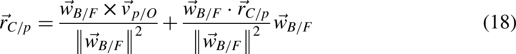
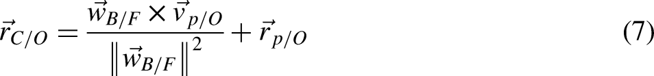
For every point

p

, there is one and only one plane on which

p

lies that is also normal to the IAR. If

C

is defined such that it also lies in that plane, as well as on the IAR, then

{\vec{r}}_{C / p}

may be calculated using equation (6). Then,

{\vec{r}}_{C / p}

must be perpendicular to

{\vec{w}}_{B / F}

, as in the planar case, and the second term on the right-hand side of equation (18) is equal to zero.

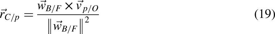
{\vec{r}}_{C / p} = \frac{{\vec{w}}_{B / F} \times {\vec{v}}_{p / O}}{{‖ {\vec{w}}_{B / F} ‖}^{2}}

(19)

Then, since the IAR must be parallel to the angular velocity vector and

C

is located on the IAR, the IAR is parallel to

{\vec{w}}_{B / F}

and passes through

C

. While it is apparent that equation (6) and equation (19) are identical, there is a significant difference in how the two equations may be interpreted for the cases of planar and three-dimensional motion. That is, for the planar case, equation (6) will yield the same location of

C

regardless of the choice of

p

. However, for three-dimensional motion, the location of

C

on the IAR, as calculated by equation (19), is dependent on the choice of

p

, as shown in Figure 5. Therefore, the method described cannot identify the specific location of the body’s fixed point. It can only identify the velocity vector along which the fixed point is translating, a vector that passes through

C

and is parallel to the angular velocity vector.

Figure 5.

Three-dimensional motion of a rigid body, showing that the angular velocity vector and the instantaneous axis of rotation (IAR) are parallel. Points $C_{i}$ are located on the IAR and correspond to points $p_{i}$ in the body.

General three-dimensional motion has analogies to the body and space centrodes which exist for planar motion. They are commonly called the body cone and the space cone,^17,4–6 and they are surfaces that may be used to describe the motion of the body. That is, it can be said that the body cone rolls on the space cone. The body cone may be determined by calculating a series of IARs in the body reference frame, as the body moves. Similarly, the space cone is identified by calculating a series of IARs in the global reference frame, as the body moves. In each case, the surfaces are defined by the IAR vectors. The process of calculating the body and space cones is more difficult than identifying the body and space centrodes and is best shown by example.

Three-dimensional example

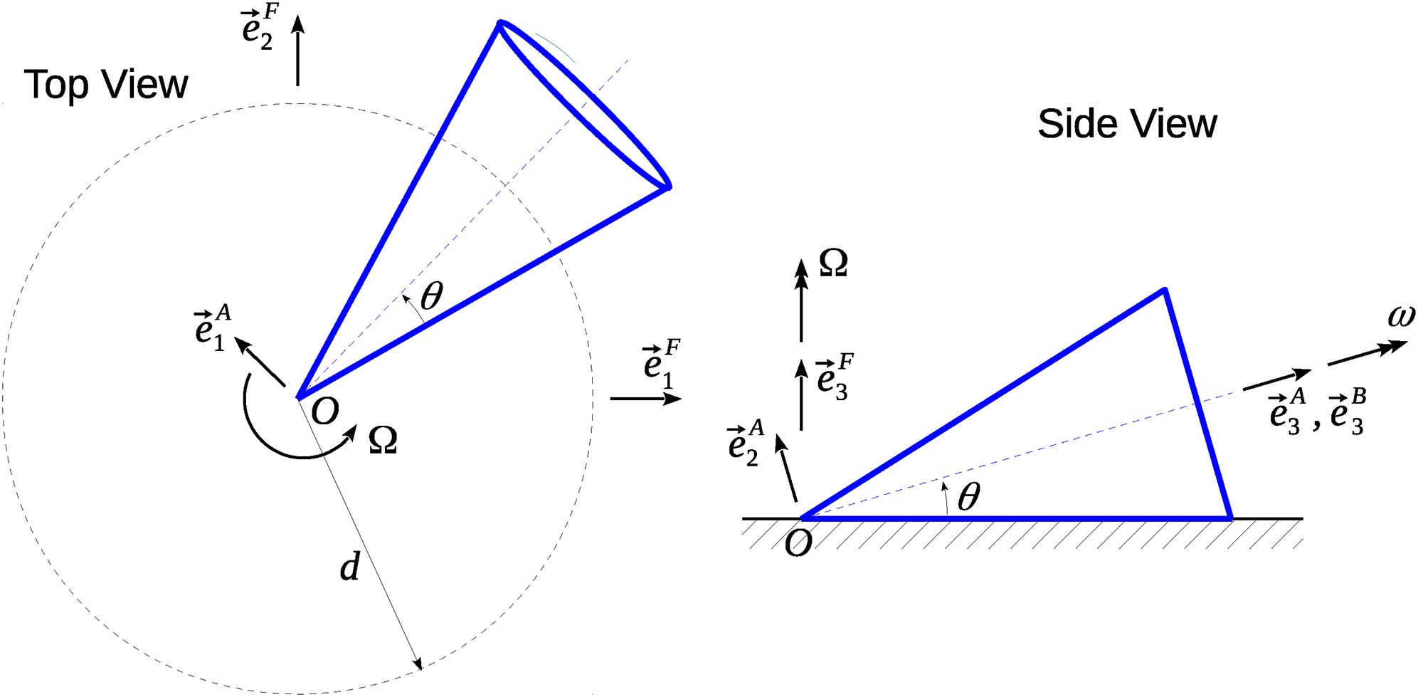
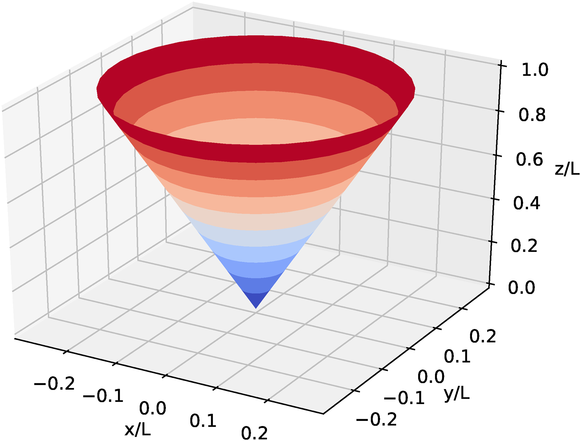
A solid, right-circular cone of length $L$ (along the ${\vec{e}}_{3}^{B}$ axis) that is rolling without slipping on a flat surface, as shown in Figure 6, will be used to demonstrate the analytical method for locating the IAR. Three reference frames are defined for the system: the $F$ frame is fixed to the flat surface, the $B$ frame is fixed to the cone, and the $A$ frame rotates about the ${\vec{e}}_{3}^{F}$ axis with the cone, but does not rotate about the ${\vec{e}}_{3}^{B}$ axis. Point $O$ is the origin of all three reference frames. Two coordinates define the position and orientation of the cone: $Φ (t)$ is the angle between ${\vec{e}}_{1}^{F}$ and the projection of ${\vec{e}}_{3}^{A}$ on the flat surface, and $ϕ (t)$ is the angle between ${\vec{e}}_{1}^{A}$ and ${\vec{e}}_{1}^{B}$ .

Figure 6.

Cone rolling without slipping on a flat surface. The cone rotates about its axis of symmetry with a constant angular velocity $ω$ , which causes the cone to also rotate about the ${\vec{e}}_{3}^{F}$ axis at a constant angular velocity $Ω$ . Point $O$ is common to the cone and the surface at all times.

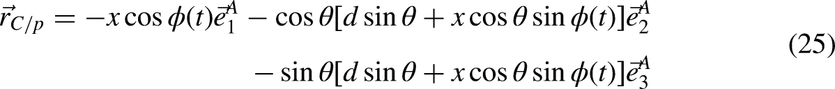
In order to derive an expression for a point $C$ located on the IAR, an arbitrary location in the cone ( ${\vec{r}}_{p / O} = d {\vec{e}}_{3}^{B} + x {\vec{e}}_{1}^{B}; x \leq d \tan θ$ ) will be used. First, an expression for ${\vec{v}}_{p / O}$ must be derived from the position of $p$ with respect to $O$ .

{\vec{r}}_{p / O} = d {\vec{e}}_{3}^{A} + x [{\vec{e}}_{1}^{A} \cos ϕ (t) + {\vec{e}}_{2}^{A} \sin ϕ (t)]

(20)

{\vec{v}}_{p / O} \equiv^{F} {\dot{\vec{r}}}_{p / O} =^{A} {\dot{\vec{r}}}_{p / O} + {\vec{w}}_{A / F} \times {\vec{r}}_{p / O}

(21)

where

{\vec{w}}_{A / F} = \dot{Φ} (t) {\vec{e}}_{3}^{F} = \dot{Φ} (t) ({\vec{e}}_{3}^{A} \sin θ + {\vec{e}}_{2}^{A} \cos θ)

\begin{aligned} {\vec{v}}_{p / O} = - {x [\dot{ϕ} (t) + \dot{Φ} (t) \sin θ] \sin ϕ (t) - d \dot{Φ} (t) \cos θ} {\vec{e}}_{1}^{A} \\ + x [\dot{ϕ} (t) + \dot{Φ} (t) \sin θ] \cos ϕ (t) {\vec{e}}_{2}^{A} - x \dot{Φ} (t) \cos θ \cos ϕ (t) {\vec{e}}_{3}^{A} \end{aligned}

(22)

The calculation of the position of point

C

on the IAR with respect to

p

using equation (19) requires

{\vec{w}}_{B / F}

{\vec{w}}_{B / F} = {\vec{w}}_{B / A} + {\vec{w}}_{A / F} = \dot{ϕ} (t) {\vec{e}}_{3}^{A} + \dot{Φ} (t) ({\vec{e}}_{3}^{A} \sin θ + {\vec{e}}_{2}^{A} \cos θ)

(23)

where

{\vec{w}}_{B / A} = \dot{ϕ} (t) {\vec{e}}_{3}^{B} = \dot{ϕ} (t) {\vec{e}}_{3}^{A}

. This a good place to introduce the no-slip condition.

\dot{Φ} (t) = - \dot{ϕ} (t) \sin θ

(24)

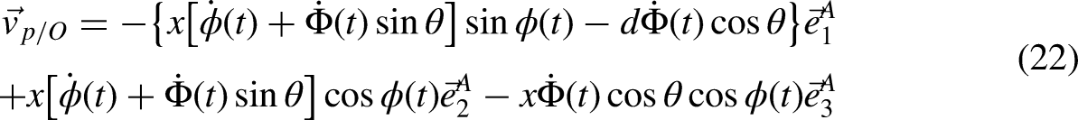
Now, substitute equation (24) into equations (22) and (23) and substitute the resulting expressions into equation (19).

\begin{aligned} {\vec{r}}_{C / p} = - x \cos ϕ (t) {\vec{e}}_{1}^{A} - \cos θ [d \sin θ + x \cos θ \sin ϕ (t)] {\vec{e}}_{2}^{A} \\ - \sin θ [d \sin θ + x \cos θ \sin ϕ (t)] {\vec{e}}_{3}^{A} \end{aligned}

(25)

It can easily be shown that the dot product of

{\vec{w}}_{B / F}

and

{\vec{r}}_{C / p}

is zero and, therefore, the two vectors are normal to one another, as required.

Now, we would like to identify the body and space cones. For the body cone, the position of $C$ with respect to $p$ will be written in terms of the $B$ reference frame basis vectors. Also, we shall assume that $x = 0$ , in order to simplify the process.

{\vec{r}}_{C / p} = - d \sin θ [{\vec{e}}_{1}^{B} \cos θ \sin ϕ (t) + {\vec{e}}_{2}^{B} \cos θ \cos ϕ (t) + {\vec{e}}_{3}^{B} \sin θ]

(26)

The simplest way to map the body cone for the entire length of the cone is to calculate values of

C

with respect to

p

from equation (26) for

0 \leq ϕ (t) \leq 2 π

and

d

between 0 and the length of the cone divided by

\cos^{2} θ

. For this problem, all points map to the surface of the rigid body cone, as one would expect. The result is shown in Figure 7. An alternative method uses the unit vectors for

{\vec{w}}_{B / F}

expressed in terms of the

B

basis vectors.

\frac{{\vec{w}}_{B / F}}{‖ {\vec{w}}_{B / F} ‖} = - {\vec{e}}_{1}^{B} \sin θ \sin ϕ (t) - {\vec{e}}_{2}^{B} \sin θ \cos ϕ (t) + {\vec{e}}_{3}^{B} \cos θ

(27)

In this method,

ϕ (t)

is varied between 0 and

2 π

in equations (26) and (27) for a single value of

d

, then the vectors that pass through the calculated values of

{\vec{r}}_{C / p}

are mapped to form a cone. One advantage of this latter method is that the fixed point for the body can be identified as the point where any two of the vectors intersect. In this problem, the fixed point is located at the apex of the cone, which confirms the known result for this problem.

Figure 7.

Body cone plotted in a vertical orientation. Point $O$ is located at the bottom of the cone, and the $z / L$ axis corresponds to the cone axis of symmetry. For this example, $θ = 15^{\circ}$ .

One method for identifying the space cone is to map ${\vec{r}}_{C / O}$ , expressed in terms of the $F$ basis vectors, for $0 \leq ϕ (t) \leq 2 π$ and $d$ between 0 and the length of the cone divided by $\cos^{2} θ$ .

{\vec{r}}_{C / O} = {\vec{r}}_{C / p} + {\vec{r}}_{p / O} = d \cos θ [{\vec{e}}_{1}^{F} \sin Φ (t) - {\vec{e}}_{2}^{F} \cos Φ (t)]; where x = 0

(28)

It is obvious from equation (28) that all points on the space cone lie in the plane defined by the

{\vec{e}}_{1}^{F}

and

{\vec{e}}_{2}^{F}

basis vectors for all values of

d

and

Φ (t)

, again as expected.

Conclusions

In this paper, a known but rarely published direct, analytical alternative to the more widely published indirect methods for calculating the ICR for a rigid body undergoing planar motion has been examined. A derivation was performed which resulted in a closed-form expression for the position of the ICR relative to a single arbitrary point on the body. Subsequently, it was demonstrated how this expression could also be used to derive closed-form expressions for the body and space centrodes for rigid body motion.

In the derivation of equation (6), it may be persuasively argued that equations (1) and (2) are unnecessary, and that one could start directly from equation (3). In fact, the indirect methods described in several texts and articles^4,5,9,11 are based on equation (3), or a close variant thereof. It would be straightforward to implement the vector cross product operation performed to obtain equation (5), which results in equation (6).

Additionally, it was shown how the direct, analytical method used to locate the ICR for planar motion could be extended to locating the IAR for general rigid body motion. This extension also led to uncovering techniques that can be used to identify the body and space cones, as well as the fixed point for the body. The use of these techniques was demonstrated by an example problem with a known solution.

Footnotes

ORCID iD

Donald L Kunz

References

Uicker

Jr. JJ

Pennock

Shigely

. Theory of Machines and Mechanisms. 5 ed Oxford University Press, New York, NY, USA, 2016. ISBN 978–0190658908.

Bernal-Torres

Medellín-Castillo

Arellano-González

. Design and control of a new biomimetic transfemoral knee prosthesis using an echo-control scheme. Journal of Healthcare Engineering 2018; 2018: Article ID 8783642. DOI: 10.1155/2018/8783642

Sun

Zheng

et al. Optimal Design of a Geared Five-Bar Prosthetic Knee Considering Motion Interference, volume 856, chapter Recent Developments in Mechatronics and Intelligent Robotics. ICMIR 2018. Advances in Intelligent Systems and Computing. Springer, Cham. ISBN 978-3-030-00213-8, 2019. pp. 828–837. DOI: 10.1007/978-3-030-00214-5_103.

Baruh

. Analytical Dynamics. 1 ed WCB/McGraw-Hill, Boston, MA, USA, 1999. ISBN 0-07-365977-0. pp. 200–202, 359–363.

Hibbeler

. Engineering Mechanics: Dynamics. 13 ed Prentice-Hall, Englewood Cliffs, NJ, USA, 2012. ISBN 978-0132911276. pp. 351–357.

Meriam

Kraige

. Engineering Mechanics: Dynamics, vol. 27 ed John Wiley and Sons, Inc., Hoboken, NJ, USA, 2012. ISBN 978-0470614815. pp. 362–364, 516–517.

Beer

Johnston

Mazurek

et al. Vector Mechanics for Engineers: Statics and Dynamics. 12 ed McGraw-Hill Book Company, New York, NY, USA, 2019. ISBN 978-1-259-63809-1. pp. 1023–1030, 1073–1074.

Tuttle

. Instantaneous axis of rotation. Am J Phys 1979; 47: 656–658. DOI: 10.1119/1.11956.

Zypman

. Instantaneous center of rotation and centrodes: Background and new examples. The International Journal of Mechanical Engineering Education 2007; 35(1): 79–90. DOI: 10.7227/IJMEE.35.1.7.

10.

Theron

WFD

. On using moments around the instantaneous center of rotation. Am J Phys 2009; 77: 918–919. DOI: 10.1119/1.3048539.

11.

Claessens

. Finding the location of the instantaneous center of rotation using a particle image velocimetry algorithm. Am J Phys 2017; 85: 185–192. DOI: 10.1119/1.4973427.

12.

Alexiou

. Instantaneous centre of rotation. http://physics.stackexchange.com/questions/212931/instantaneous-centre-of-rotation (2015, Accessed January 2019).

13.

Alexiou

. Centre of instantaneous rotation problem. https://physics.stackexchange.com/questions/95486/centre-of-instantaneous-rotation-problem (2014, Accessed January 2019).

14.

Peraire

Widnall

. Lecture l21 - 2d rigid body dynamics. https://ocw.mit.edu/courses/aeronautics-and-astronautics/16-07-dynamics-fall-2009/lecture-notes/MIT16˙07F09˙Lec21.pdf (2008, Accessed 28 May 2020).

15.

Chasles

. Note sur les propriétés générales du système de deux corps semblables entr’eux (in French). Bulletin des Sciences Mathématiques - Astronomiques, Physiques et Chemiques 1830; 14: 321–326.

16.

Jackson

. The instantaneous motion of a rigid body. Am Math Mon 1942; 49(10): 661–667. DOI: http://links.jstor.org/sici?sici=0002-9890.

17.

Peraire

Widnall

. Lecture l25 - 3d rigid body kinematics. hrtps://ocw.mit.edu/courses/aeronautics-and-astronautics/16-07-dynamics-fall-2009/lecture-notes/MIT16˙07F09˙Lec25.pdf (2008, Accessed 28 May 2020).