Classroom demonstration of a stagnation flow using cell phone-captured particle image velocimetry data

Abstract

Courses in fluid mechanics and aerodynamics often require lengthy and involved mathematical derivations. However, these subjects are also associated with visually appealing flow features. In an effort to provide students with a full appreciation for fluid mechanics, it is desirable to not only provide a theoretical background, but also perform some visual demonstrations; this can be achieved through quantitative flow visualization demonstration. The cost of research-grade equipment is prohibitive for a teaching college, especially if only used for classroom demonstration. This article describes a Particle Image Velocimetry (PIV) demonstration of flow around a vertical plate using widely available cell phone cameras, reducing the cost of the required equipment. The velocity field calculated using PIV analysis was compared to a velocity field predicted using potential flow theory. The two showed an agreement of about 30% – a sufficient accuracy for an in-classroom demonstration. The learning effectiveness of this demonstration was evaluated using course evaluations and an end-of-semester survey. Overall, students expressed their appreciation for added experimental work and visualization to the course curriculum.

Keywords

Cell phone particle image velocimetry mobile phone cameras flow around vertical plate experimental techniques in-class experiment potential flow particle image velocimetry

Introduction

Upper division and graduate fluid mechanics courses often involve extensive mathematical derivation, which can make classroom lectures mundane. To dilute this mathematically-focused classroom time, instructors turn to more hands-on activities. These include projects based on the numerical simulations^1,2 and experimental demonstrations.^3,4 Special attention has been given to flow visualization demonstrations, which utilize the appealing visual nature of flowing fluid to encourage students’ interest in the subject.^5–8 Pedagogy in fluid mechanics courses can benefit from a hands-on demonstration using Particle Image Velocimetry (PIV), which combines the visual representation of the flow with quantitative analysis. This classroom exercise would promote active learning⁹ and demonstrate a modern experimental technique to students. The visual aspect of PIV analysis can also encourage less scientifically inclined students to appreciate fluid mechanics^10,11 and encourage life-long learning.⁸ A typical PIV setup consists of a high-intensity LASER that illuminates flow seeding particles whose motion is captured using a high-speed camera. Processing software is then used to convert the motion of the particles into velocity field data. A modern PIV system can cost on the order of tens of thousands of dollars,¹² making this demonstration financially prohibitive for a common teaching college. The requirement for research-grade equipment can be eliminated by studying a relatively low-speed flow, which can be achieved by using low-frame rate video. In this case, now widely available cell phones can be used to capture sufficiently good data for a demonstration. The ever-increasing light sensitivity of these cameras and the current frame rate make it also possible to replace the high-intensity LASER with a cheaper option. In this article we describe the feasibility of performing a quantitative flow visualization classroom demonstration using a cell phone camera (or more aptly named “smart phone”) to capture the flow around a flat plate.

Utilizing cell phones as a replacement for high-speed cameras is an area of increasing interest for PIV analysis. Within the past few years, this concept has been applied in praxis to demonstrate the viability of using cell phones for visual flow quantification. Cierpka et al.¹³ analyzed a water jet with a mean flow of about 92 mm/s. The authors used a cell phone comparable to an iPhone 6 to capture images, and resultant PIV analysis data was compared to data obtained using the pco.dimax HS4 high-speed camera. They found that the mean difference in the velocities were under 1.5 mm/s in both the axial and radial velocity components. The use of cell phones for PIV systems also has great potential for larger-scale and more complex experiments; this has already been implemented in several studies. Large scale Particle Image Velocimetry (LSPIV) has been used to analyze the surface velocity of a river upstream catchment located on the Shihmen Reservoir.¹⁴ The data captured from the cell phone were compared to measurements from a handheld digital flow meter. The advances in cell phone technology also enable cell phone processors to perform PIV analysis locally, meaning all PIV analyses are performed on the device without needed external software. For example, Armijo et al.¹⁵ are developing a smartphone applet called Mobile Instructional Particle Image Velocimetry (miPIV), which is capable of performing PIV analysis. Beat et al.¹⁶ analyzed a small-open channel of a river with a mean velocity of 340 mm/s. These authors analyzed data using an application in the alpha stage of development on a Huawei Ascend Y300 cell phone, and resultant PIV analysis data was compared to a commercial radar sensor. The authors listed a deviation of less than 10% between captured surface velocities. A more complex analysis performed by Aguirre-Pablo et al.¹⁷ utilized tomographic PIV by capturing the flow of a vortex ring being produced by a pressurized pulse through a circular orifice in water with a mean flow of 200 mm/s. Four separate cell phones (Nokia Lumia 1020) were used, and the resultant PIV analysis data was compared to data obtained using Imager-Pro-X dual-frame CCD. These authors found a relative error of less than 15% between obtained velocity magnitudes.

First, in the next section, the relevant potential theory will be discussed. Subsequently, the experimental equipment, suitable for a classroom environment, and procedure are described. Finally, experiment and theory are compared and effects of the demonstration on the student learning is discussed.

Theoretical considerations

The flow around a vertical plate can be constructed using potential theory. This is a topic which is usually covered in aerodynamics courses, so this exercise fits well into the overall curriculum. For completeness, the theoretical derivation of the potential flow around a vertical plate is described next.

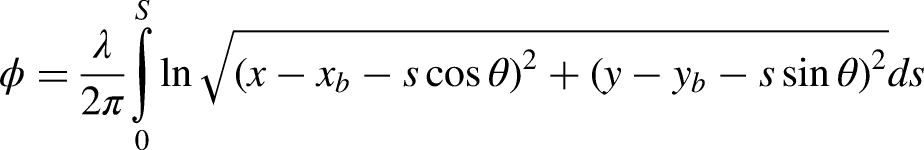
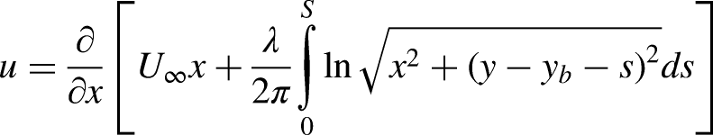
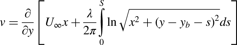
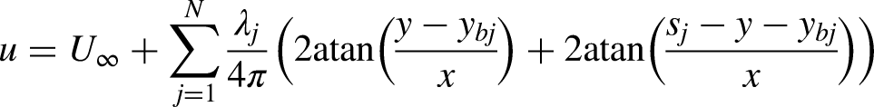
This flow can be constructed by placing several source panels in a uniform flow.¹⁸ The potential function, $ϕ$ , for the horizontal free stream velocity is

ϕ = U_{\infty} x

where

u \equiv \frac{\partial ϕ}{\partial x}

and

v \equiv \frac{\partial ϕ}{\partial y}

and

U_{\infty}

is the freestream velocity. The velocity potential for a single source line originating at coordinates

(x_{b}, y_{b})

, length S and an angle

θ

with respect to horizontal imaginary line, and strength

λ

ϕ = \frac{λ}{2 π} \int_{0}^{S} \ln \sqrt{{(x - x_{b} - s \cos θ)}^{2} + {(y - y_{b} - s \sin θ)}^{2}} d s

The upstream flow around a vertical flat plate can be approximated by placing a single source line with starting boundary point

(0, y_{b})

, length S, and strength

λ

in the uniform flow as shown in Figure 1.

Figure 1.

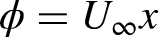
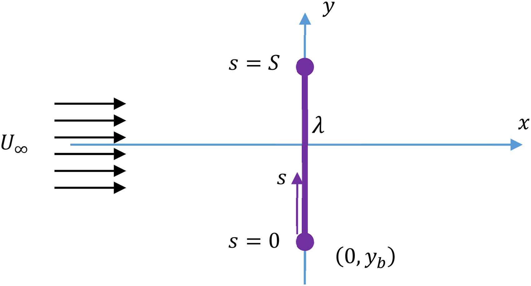
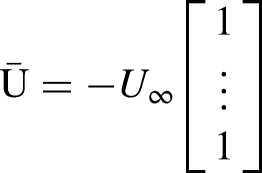
Flow around a vertical plate can be simulated by superimposing a uniform flow of speed $U_{\infty}$ with a line source of strength $λ$ .

The plate is vertical and forms angle $θ = \frac{π}{2}$ with the horizontal reference line, simplifying the expression to:

ϕ = U_{\infty} x + \frac{λ}{2 π} \int_{0}^{S} \ln \sqrt{x^{2} + {(y - y_{b} - s)}^{2}} d s

The expressions for the velocity field can be found by differentiating the resultant potential function:

u = \frac{\partial}{\partial x} [U_{\infty} x + \frac{λ}{2 π} \int_{0}^{S} \ln \sqrt{x^{2} + {(y - y_{b} - s)}^{2}} d s]

v = \frac{\partial}{\partial y} [U_{\infty} x + \frac{λ}{2 π} \int_{0}^{S} \ln \sqrt{x^{2} + {(y - y_{b} - s)}^{2}} d s]

Evaluating the partial derivative and the integral for each component yields:

u = U_{\infty} + \frac{λ}{4 π} \cdot (2 atan (\frac{y - y_{b}}{x}) + 2 atan (\frac{s - y - y_{b}}{x}))

v = - \frac{λ}{4 π} [\ln (s^{2} - 2 y y_{b} - s (2 y - 2 y_{b}) + x^{2} + y^{2} + y_{b}^{2}) - \ln (x^{2} + y^{2} - 2 y y_{b} + y_{b}^{2})]

Instead of a single vertical panel, a more realistic model to represent this flow can be obtained by positioning multiple panels in the flow as shown in Figure 2. Each panel has a distinct boundary starting point

(0, y_{b j})

, length

S_{j}

and strength

λ_{j}

. Combining a uniform flow with N panels, yields:

ϕ_{j} = U_{\infty} x + \sum_{j = 1}^{N} \frac{λ_{j}}{2 π} \int_{0}^{s_{j}} \ln \sqrt{x^{2} + {(y - y_{b j} - s_{j})}^{2}} d s_{j}

with velocity components:

u = U_{\infty} + \sum_{j = 1}^{N} \frac{λ_{j}}{4 π} (2 atan (\frac{y - y_{b j}}{x}) + 2 atan (\frac{s_{j} - y - y_{b j}}{x}))

v = \sum_{j = 1}^{N} - \frac{λ_{j}}{4 π} [\ln (s_{j}^{2} - 2 y y_{b j} - s_{j} (2 y - 2 y_{b j}) + x^{2} + y^{2} + y_{b j}^{2}) - \ln (x^{2} + y^{2} - 2 y y_{b j} + y_{b j}^{2})]

Figure 2.

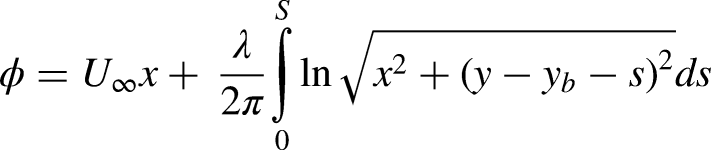
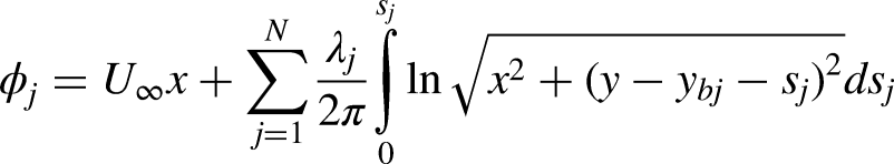
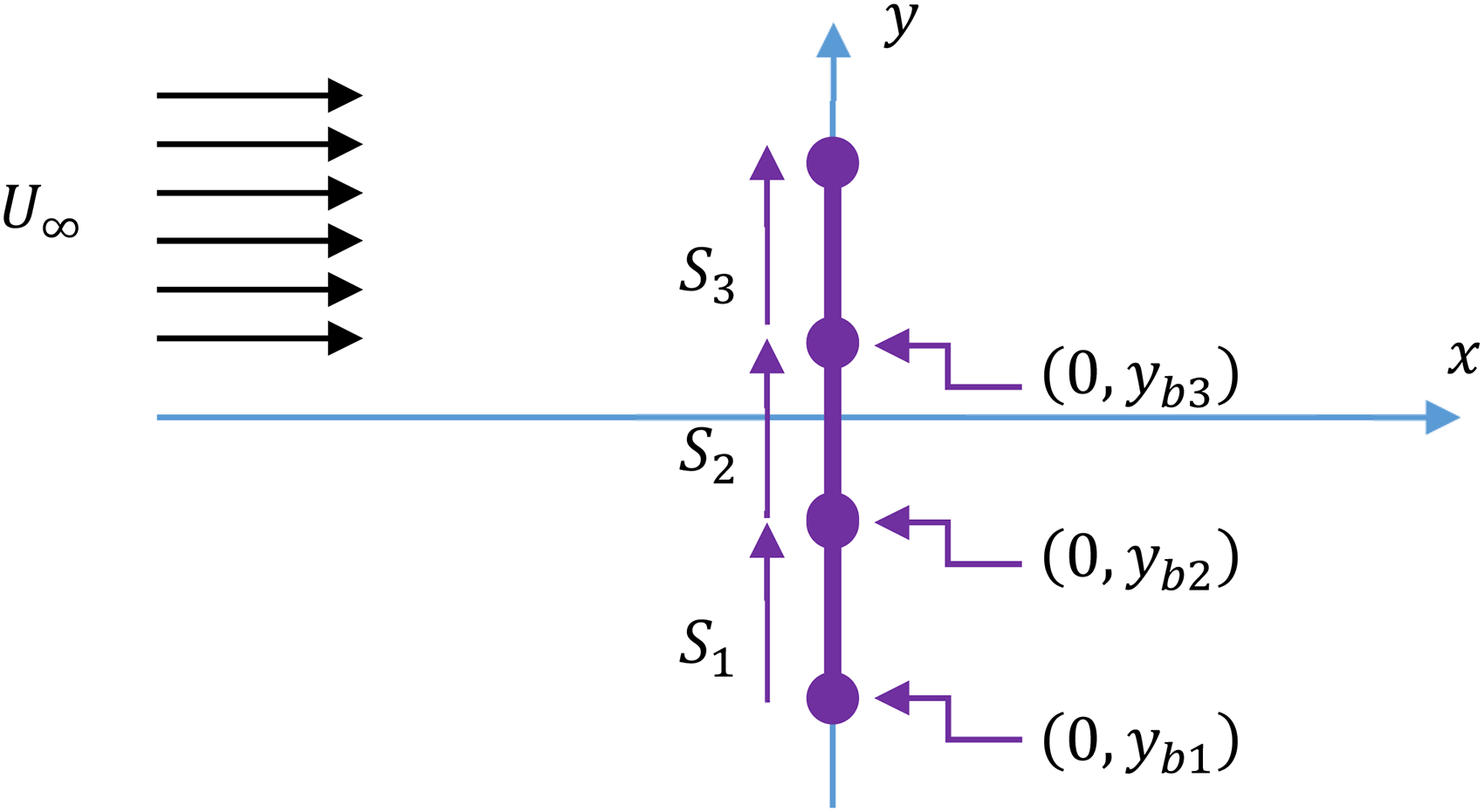
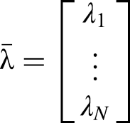
A more accurate representation can be achieved by including several source lines, each of distinct strength.

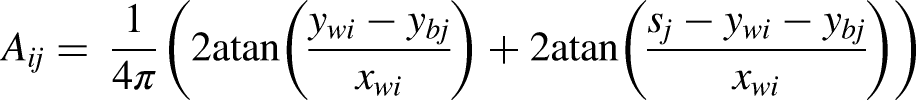
A boundary condition can be used to solve for the appropriate source strength for each panel by setting the local horizontal velocity component at the location of the virtual wall $(x_{w}, y_{w})$ to zero as shown in Figure 3. This leads to the following expression:

\sum_{j = 1}^{N} \frac{λ_{j}}{4 π} (2 atan (\frac{y_{w} - y_{b j}}{x_{w}}) + 2 atan (\frac{s_{j} - y_{w} - y_{b j}}{x_{w}})) = - U_{\infty}

Figure 3.

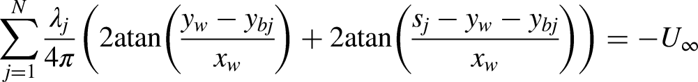
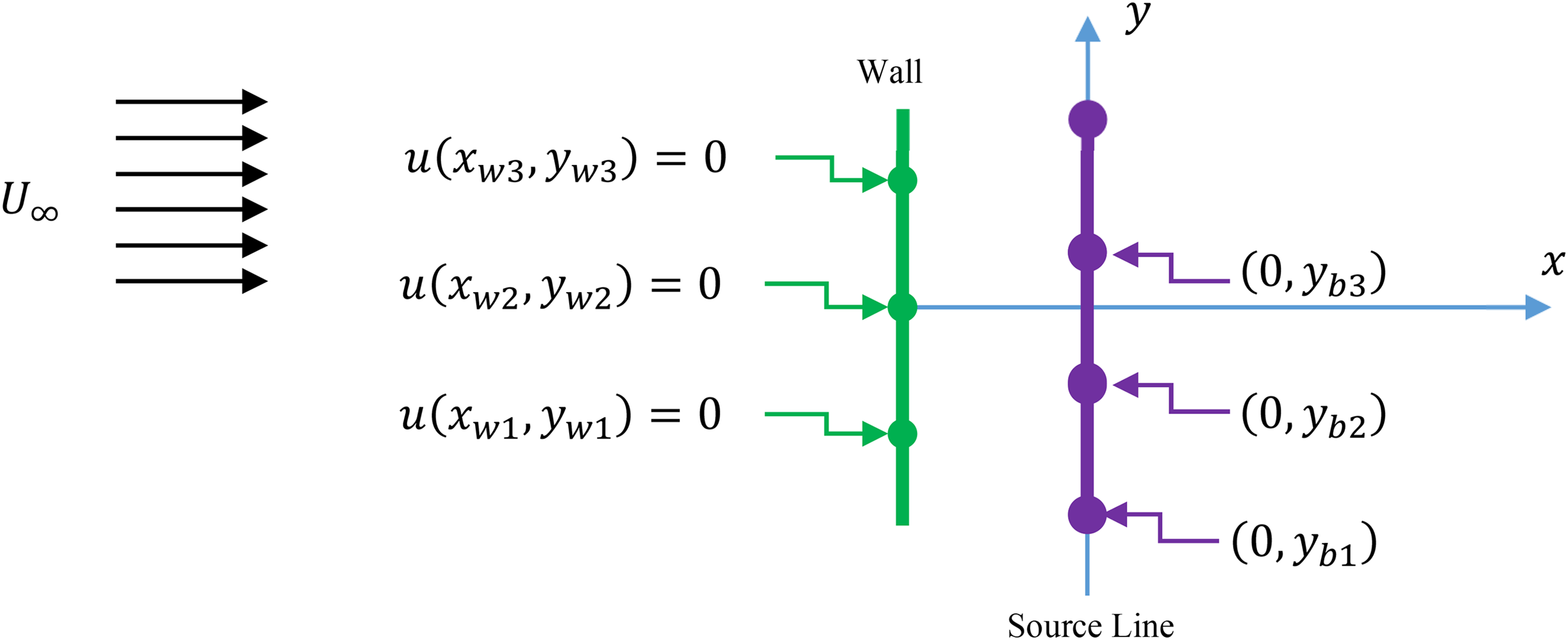
Stagnation boundary condition at the location of the vertical plate is required to solve for unknown $λ^{'} s$ .

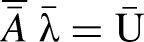
Writing out the same boundary condition for all panels on the virtual wall forms a system of $N$ equations:

\bar{\bar{A}} \bar{λ} = \bar{U}

where

A_{i j} = \frac{1}{4 π} (2 atan (\frac{y_{w i} - y_{b j}}{x_{w i}}) + 2 atan (\frac{s_{j} - y_{w i} - y_{b j}}{x_{w i}}))

\bar{U} = - U_{\infty} [\begin{matrix} 1 \\ ⋮ \\ 1 \end{matrix}]

and

\bar{λ} = [\begin{matrix} λ_{1} \\ ⋮ \\ λ_{N} \end{matrix}]

\bar{λ}

can be found using matrix inversion.

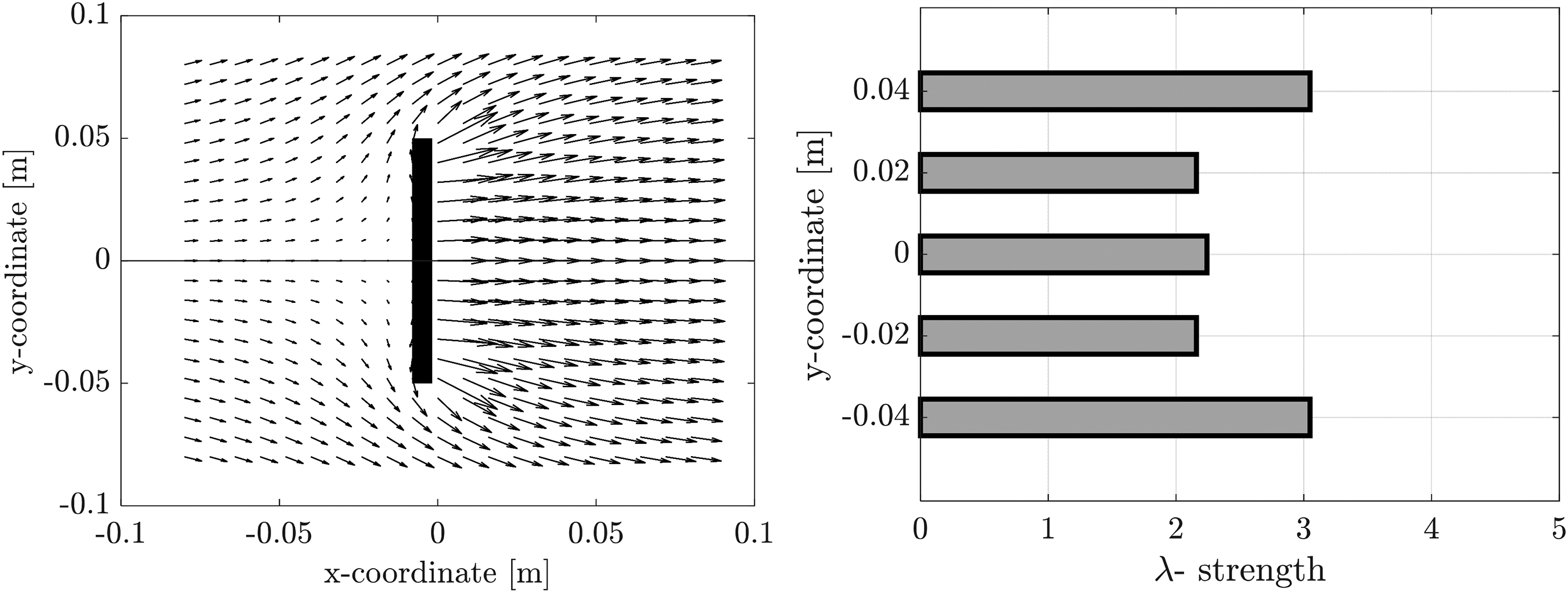
A sample flow around a flat plate is shown in Figure 4, which was created using five panels placed normal to a $1 m / s$ free stream flow. The $λ$ distribution over the entire plate is also shown in the same figure.

Figure 4.

(Left) Sample solution for a flow around a vertical plate and (right) the associated λ source strength distribution.

Experimental setup

The experiment was performed inside a 10-gallon fish tank filled with water that was seeded using 9–13 $μ m$ silica glass beads providing about $5 p / m m^{2}$ seeding density. A flat, black plate was attached to a frame that could be easily dragged across the top rim of the fish tank producing a relatively uniform flow over the plate. The resultant flow relative to the plate was about $10 c m / s$ (in the future, attaching a linear motor that ensures a uniform motion of the plate is recommended). The water level in the tank was sufficient to submerge the plate completely and produce a symmetrical flow of water over all sides of the plate. The frame, which was holding the flat plate, was also attached to a cell phone holder, such that there was no net relative motion of the plate in the field of view of the cell phone. The silica particles were illuminated using a green LASER pen beam reformed into a sheet using a 5-mm cylindrical lens as shown in Figure 5. The lights in the room were dimmed and the cell phone camera was focused on the particles illuminated by the LASER sheet. The frame was then dragged across the fish tank while the camera captured images in the burst mode. The camera used in this experiment was an iPhone 6s. The timestamp associated with each captured frame was deduced based on the frame number and the capture frame rate. The frame rate of the camera was confirmed by using a burst mode to capture images of a timer. The difference in values of the timer recorded in each frame was then used to compute the mean and standard deviation of the sample rate. For the iPhone 6s, the mean rate was 13.6 Hz and standard deviation was 10.1 Hz. For reference, we also used same methods to measure the mean frame rate and standard deviation of other available devices, listed in Table 1.

Figure 5.

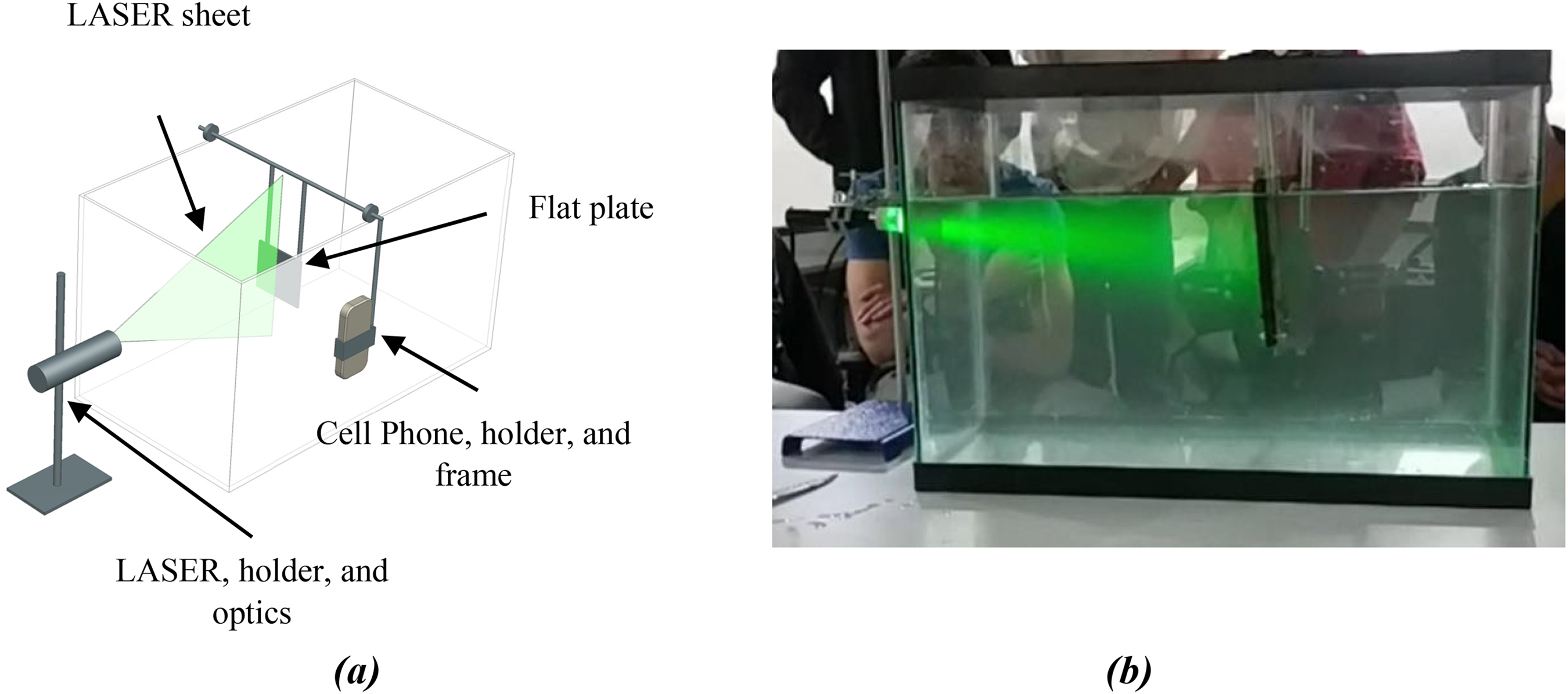
(a) Schematic of the experimental apparatus; (b) picture of the demonstration setup.

Table 1.

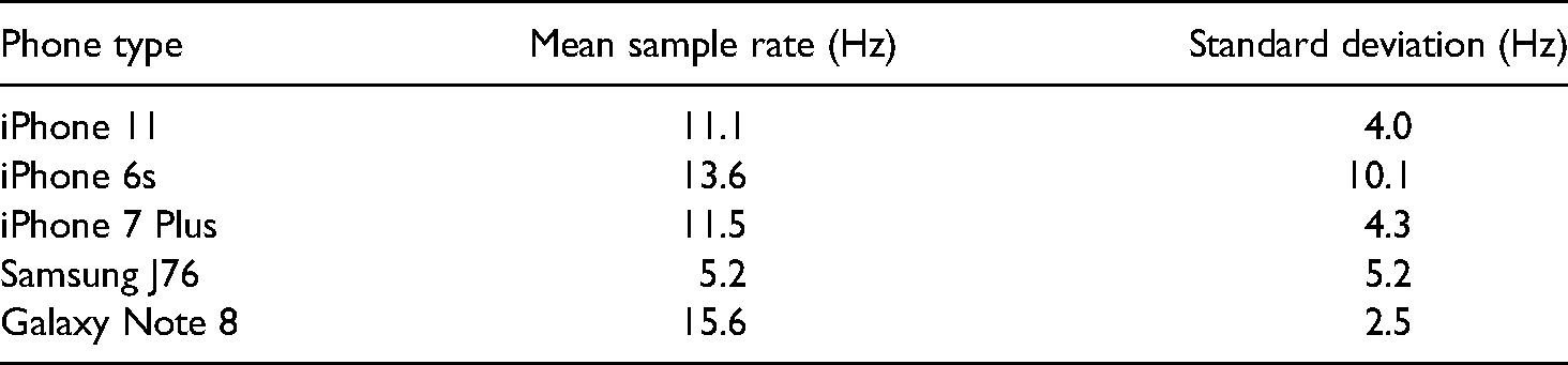
Picture capturing characteristics of modern cell phones.

Phone type	Mean sample rate (Hz)	Standard deviation (Hz)
iPhone 11	11.1	4.0
iPhone 6s	13.6	10.1
iPhone 7 Plus	11.5	4.3
Samsung J76	5.2	5.2
Galaxy Note 8	15.6	2.5

A MATLAB PIVLab applet^19,20 was used to process images captured by the cell phone and to calculate the velocity field. The usage of MATLAB was welcomed by students as they already used it extensively in the course for their analytical calculations. Introducing them to a PIVLab proved easy as students already possessed required knowledge of the MATLAB programming language from the course. All students were asked to write their own codes to process the output files provided by the PIVLab. The raw cell phone image was 3024 × 4032 pixels and 3.61 MB in digital size. 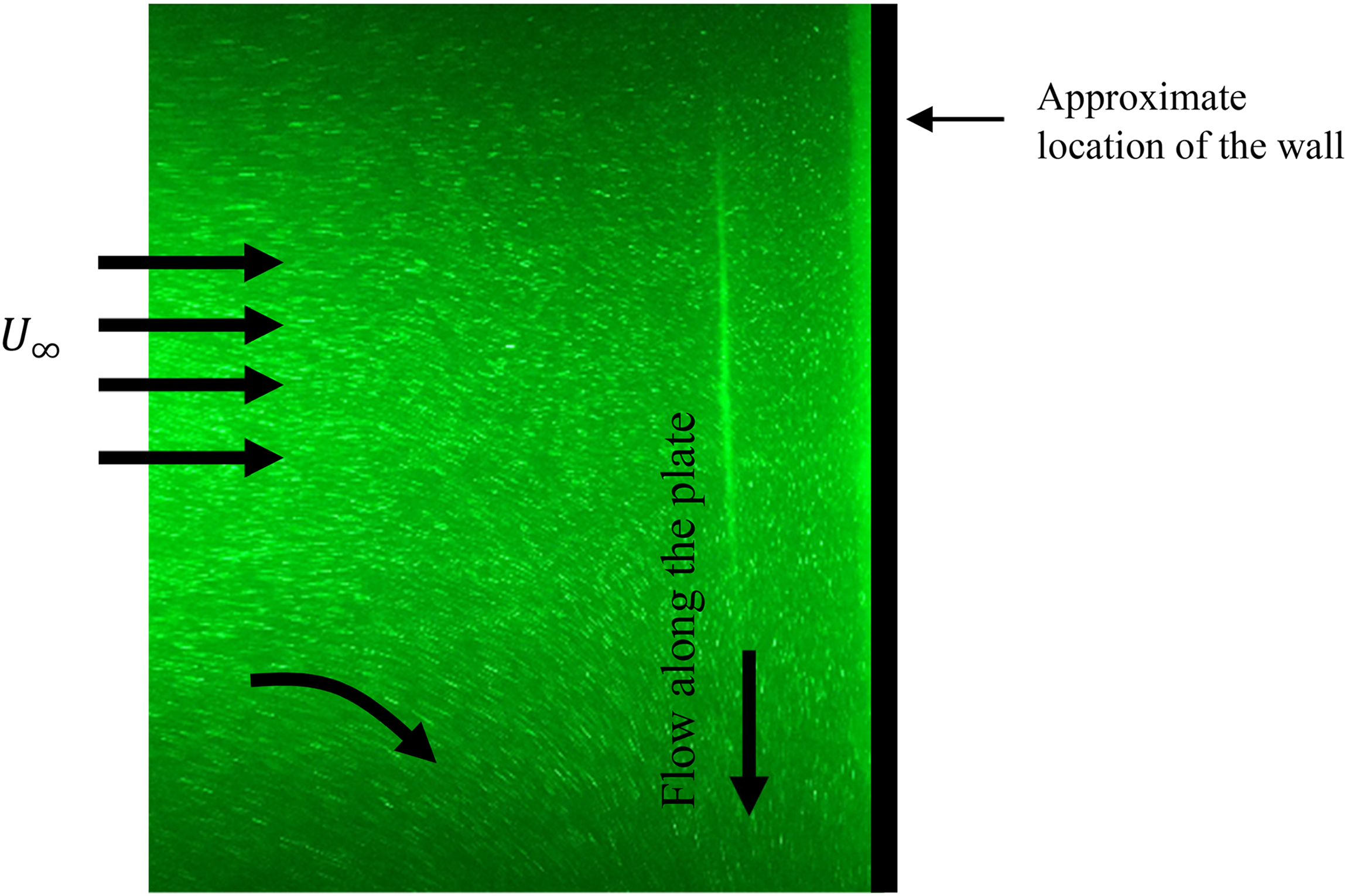After identifying a region of interest, a double pass FFT window deformation algorithm was used with an interrogation zone of $600 \times 600$ -pixel and $300 \times 300$ -pixel interrogation zones resulting in a velocity field with $d x = d y = 4.2 m m$ spatial resolution. Figure 6 shows a sample image captured by the camera. In this image, the flow velocity was increased to observe the particle streaking, in order to clearly indicate the flow direction in the image.

Figure 6.

Sample raw image captured by a cell phone camera.

Overall, the setup time for the demonstration took about an hour prior to the class. This included filling up the fish tank with water and adjusting the seeding particle concentration to optimize the PIV data collection. The demonstration itself took about 30 min during which several passes of the plate in the fish tank were taken. A quick demonstration of data processing using PIVLab followed; the actual processing of data was assigned as homework. The cleanup also took about an hour, which included emptying the fish tank and disassembling the setup.

Results

The results are based on the homework, which required students to perform a PIV analysis and compare the velocity field to the potential flow theory prediction. Figure 7 shows a sample result with green vectors indicating velocity obtained using PIV analysis and black vectors corresponding to velocity obtained using potential flow theory. The thick black line indicates the approximate location of the physical wall, and the red dot indicates the approximate location of the stagnation point. Data in the near-wall region were omitted due to significant differences between the experimental and theoretical velocity field. The error was partially attributed to poor PIV data near the wall where LASER reflection and background light polluted the view. The fact that theoretical calculations do not account for the viscous effect in the near-wall region was discussed with students. The mean difference between the experimentally and theoretically obtained axial velocity component is about 30% of the free stream velocity. Although this difference would render the result not accurate for the research analysis, this is sufficiently good for an in-classroom demonstration as it clearly shows the trend of the flow, which agrees with the theoretical analysis. Moreover, the overall qualitative representation of the flow field is satisfactory.

Figure 7.

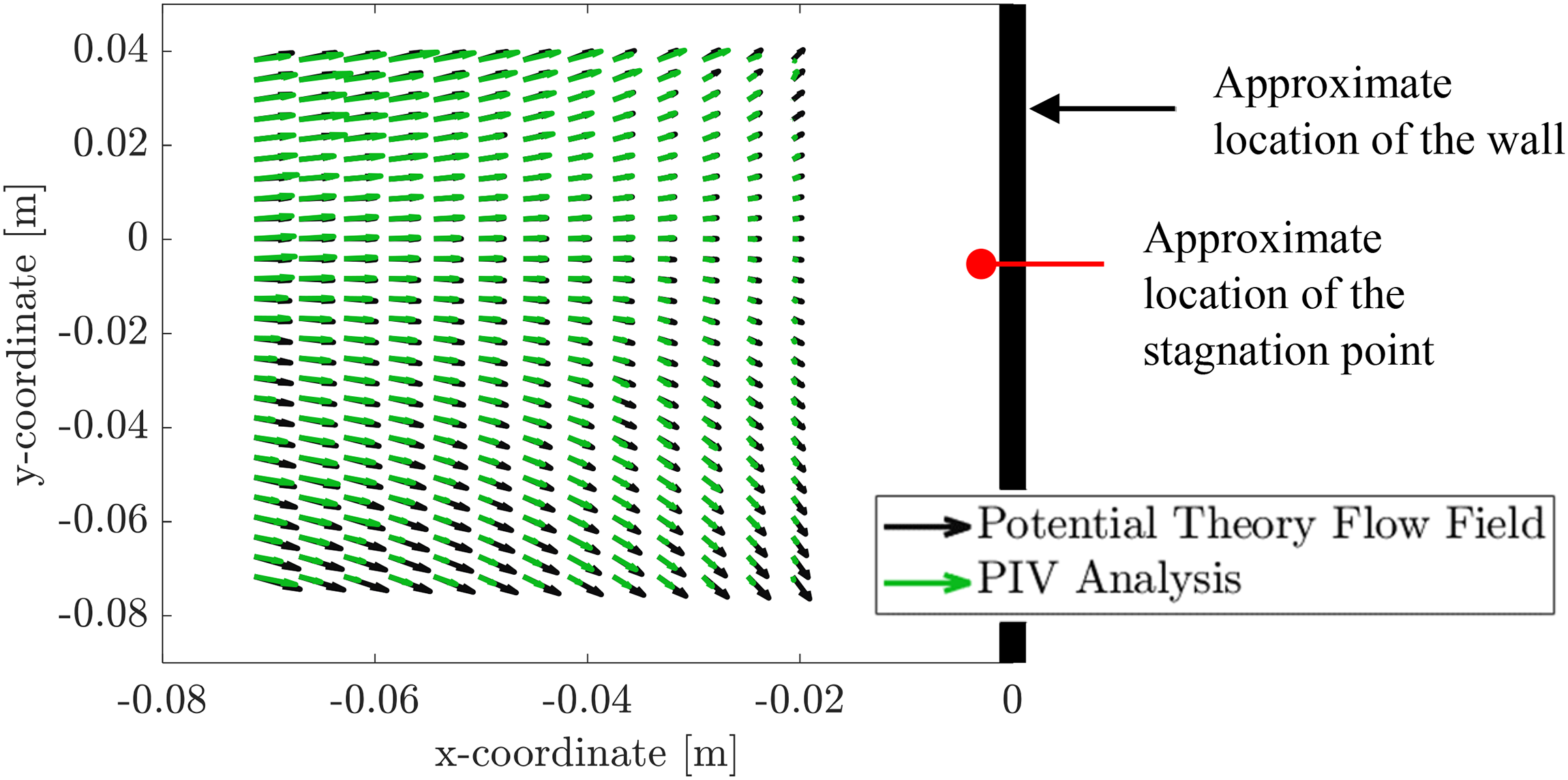
Comparison between the flow field computed using PIV experimental data (green vector) and the one predicted using potential flow theory (black vectors).

The major objectives of this exercise were to 1) dilute the analytical classroom work with flow visualization demonstration 2) introduce modern experimental techniques in fluid mechanics. During the five years in which the course was offered to about 20 students per semester, the experimental work was included twice. Student course evaluations were examined to identify how the experimental work affected students’ learning. During the two years which included the experimental demonstration, students reflected positively on the activity. This was primarily evident in the evaluation question: “What aspects of this course were most beneficial to you?”. Some of the comments are included: Student 1:

“Both the numerical and experimental validation of an analytical solution really reinforced my understanding of the material.”

Student 2:

“This is easily one of my favorite courses that I've taken at Manhattan College and I really liked the way that it was taught. Being able to generate theoretical flow fields using MATLAB, run experiments in class, process the results, and then compare theoretical and experimental data was definitely a huge benefit of this course.”

Meanwhile, there were no negative comments found corresponding to question “How can this course be improved?”.

In combination with the course evaluations, a separate survey was distributed to all students to evaluate the experimental work alone. Overall, 90% of all students enjoyed performing the experiment. Moreover, 90% of the students enjoyed the experimental aspect the exercise introduced into the course and only 10% of the class would rather perform a computational analysis to visually demonstrate theoretical concepts. The main goal of this exercise was to introduce students to modern quantitative flow visualization techniques. It is far from obvious that any of the students will use the PIV method after graduating from college. However, when asked about the usefulness of learning modern experimental techniques, 83% of students replied that they hoped to use it their future career. The rest of the students found it unlikely that they would use PIV in their future work, however agreed that they enjoyed learning a new method. A typical survey outcome is presented in Appendix A. Overall, the exercise proved to be a success.

Conclusion

In this article we demonstrated an in-class exercise that is used in Manhattan College as a part of a graduate aerodynamics course. The goal is to introduce students to a modern flow visualization technique by performing a PIV experiment of a flat plate flow. Considering the high cost of research-grade PIV equipment, the authors demonstrated a much more economical setup using widely available cell phones. The experimental data was compared to the predictions made using potential flow theory, a topic which aligns well with the curriculum of the upper division or graduate aerodynamics course. It was shown that the velocity field predictions and the experimental flow field came in sufficient agreement for a classroom demonstration. In a course evaluation survey, students expressed overall satisfaction with the experimental work added to the course and appreciation for learning a new modern experimental technique.

Footnotes

Declaration of conflicting interests

The author(s) declared no potential conflicts of interest with respect to the research, authorship, and/or publication of this article.

Funding

The author(s) received no financial support for the research, authorship and/or publication of this article.

ORCID iDs

Oleg Goushcha

Shalin Angira

Appendix A

During the experiment you learned basics of the PIV method. What are your feelings about learning a new experimental method?

References

Zamora

Kaiser

Vicente

. Improvement in learning on fluid mechanics and heat transfer courses using computational fluid dynamics. Int J Eng Ed 2012; 38: 147–166.

Navaz

Henderson

Berg

. A New Approach to Teaching Undergraduate Thermal/Fluid Sciences - Courses in Applied Computational Fluid Dynamics and Compressible Flow. Int J Mech Eng Educ 2002; 30: 35–49.

Naylor

. William Roy Penney and Edgar C Clausen (Eds), Fluid mechanics and heat transfer: inexpensive demonstrations and laboratory exercises. Int J Mech Eng Educ 2018; 47: 382–383.

Macías-Machín

Henríquez

Lozano

. A simple experiment on heat transfer using a phase change material. Int J Mech Eng Educ 1996; 24: 119–123.

Goushcha

. Revival of water table experiments in fluid mechanics courses, part I. Int J Mech Eng Educ 2019; 48(3): 284–293.

Jensen

. Fluid mechanics: there's an app for that. Logan, UT: Utah State University, 2018.

Linke

Martin

Garretson

. Learning benefits by integrating design, manufacturing, and testing in a course for compressible flow visualizations. Int J Mech Eng Educ 2020; 48: 297–314.

Hertzberg

Sweetman

. A course in flow visualization: the art and physics of fluid flow. Boulder: University of Colorado, 2004.

Grant

. The effective use of laboratories in undergraduate courses. Int J Mech Eng Educ 1995; 23: 95–101.

10.

Hertzberg

. Images of fluid flow: art and physics by students. J Vis 2005; 8: 1–8.

11.

Wolff

. Visualization as a tool for physics education. Comput Phys 1991; 5: 278–286.

12.

Ring

Atkinson

Henderson

, et al. Development of a low cost particle image velocimetry system for fluids engineering research and education. ASME 2013 Fluids Engineering Division Summer Meeting. Incline Village, Nevada, 2013.

13.

Cierpka

Hain

Buchmann

. Flow visualization by mobile phone cameras. Exp Fluids 2016; 57.

14.

Liu

Huang

. Large scale particle image velocimetry measurement of river surface velocity based on images captured by a camera of the mobile phone. 22nd EGU General Assembly, 2020.

15.

Armijo

Caldwell

Mukherjee

, et al. Smartphone PIV. APS Division of Fluid Dynamics. Seattle, WA, 2019.https://ui.adsabs.harvard.edu/abs/2019APS..DFDS11008A

16.

Beat

Philippe

Peña-Haro

. Mobile device app for small open-channel flow measurement. 7th Intl. Congress on Env. Modelling and Software. San Diego, 2014.

17.

Aguirre-Pablo

Alarfaj

, et al. Tomographic particle image velocimetry using smartphones and colored shadows. Sci Rep 2017; 7: 3714.

18.

Anderson

. Fundamentals of aerodynamics. Boston: McGraw-Hill, 2001.

19.

Thielicke

Sonntag

. Particle image velocimetry for MATLAB: accuracy and enhanced algorithms in PIVlab. J Open Res Softw 2021; 9.

20.

Thielicke

Stamhuis

. PIVlab – towards user-friendly, affordable and accurate digital particle image velocimetry in MATLAB. J Open Res Softw 2014; 2.