Forced convection between parallel plates with third kind boundary condition: An asymptotic solution

Abstract

An asymptotic analysis to the Cartesian Graetz problem with third-kind boundary conditions is carried out, the temperature profile is calculated for small values of the Biot number. The analysis is performed using asymptotic matching and shows that there are two scales for the axial coordinate, which allows us to find an analytical expression for the temperature field along the channel. This expression can be easily applied in thermal engineering applications.

Keywords

Graetz problem asimptotic matching biot number

Introduction

Heat transfer in ducts that carry fluids is of great importance in the field of engineering, due to the countless applications that involve the transport of fluids through ducts and their heat exchange with the surrounding environment. One of the first approaches to mathematically model these systems is the one-dimensional or lumped parameter approach. Unfortunately, this analysis does not provide relevant information regarding the heat transfer at the walls of the duct (Nusselt Number). An improvement to this approach was introduced by Graetz in 1885,^1–7 who considered a laminar flow fully developed in a duct with a circular cross-section and determined the heat transfer between the fluid and the duct wall. This model initiated a new line of research that has continued to evolve to this day.

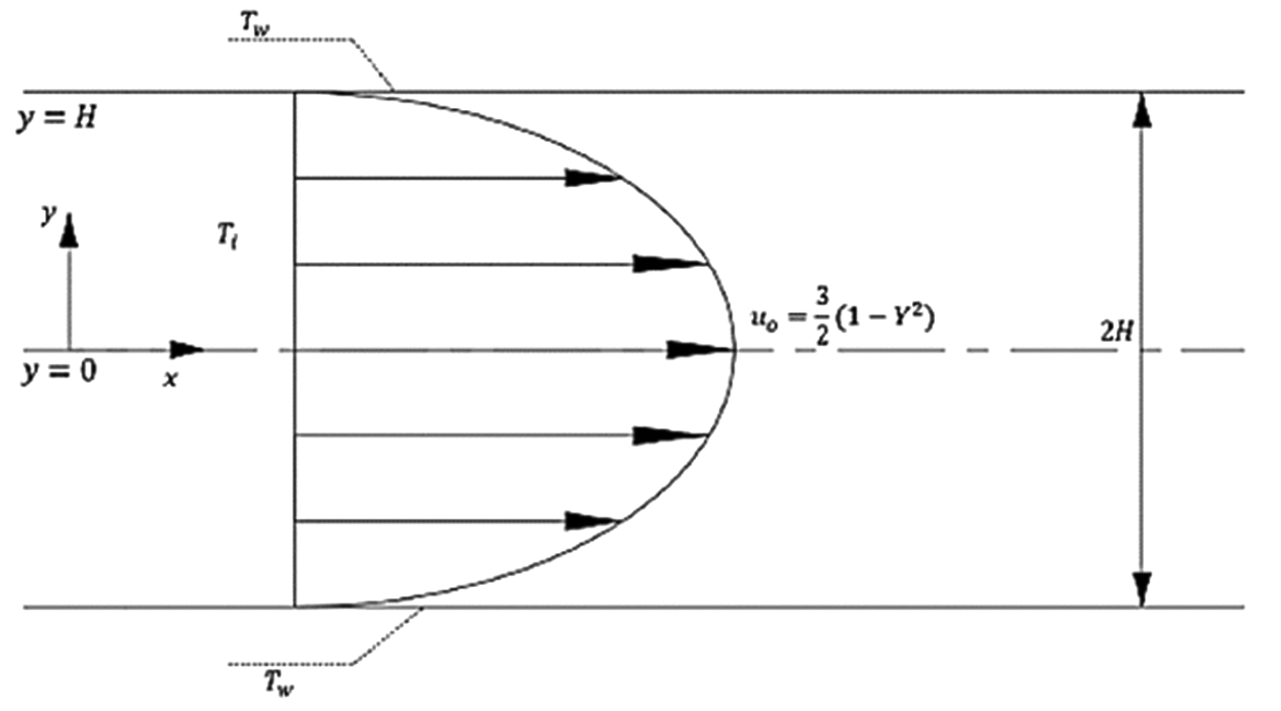
Originally, Graetz considered a constant temperature at the duct wall (Figure 1). Subsequently, several authors have expanded the problem in different ways, for example, by changing the boundary conditions on the walls,^8–15 incorporating axial conduction (extended Graetz problem), and addressing other extensions, including turbulent flows and non-Newtonian fluids.

Figure 1.

Diagram showing Graetz's problem.

The standard mathematical methodology to address these problems is the separation of variables method, which gives rise to Sturm-Liouville type problems. The boundary conditions of the problem generally lead to series solutions, which ultimately must be evaluated numerically. The accuracy of the results depends on the number of terms used in the series; these types of solutions generally require a large number of terms in regions near the channel entrance.

For example, using this technique, Prins et al.⁸ solved the Graetz Problem with a fixed-temperature condition on the walls of a flat channel, while Cess et al.¹⁶ addressed the same problem but under constant heat flux conditions on the channel walls. The case with convective boundary conditions between the channel walls and the external environment was studied by De Bye et al..⁹. Another alternative to solve Graetz-type problems is the finite difference method,¹⁵ which, like the separation of variables method, requires a very refined mesh at the channel entrance to achieve good numerical accuracy.

Another alternative to solve this type of problem is to use asymptotic or perturbation methods. This type of analysis is generally based on the existence of a small parameter in the equations that govern the process under study. For example, for small values of the Biot number, which can be interpreted as the case when the external natural convection coefficient is low, it is possible to perform a perturbation analysis.

Perturbation theory allows engineers to obtain approximations to complex problems, starting with a more simplified problem and later improving the solution through successive approximations. The main advantage of perturbation theory is that it provides approximate analytical solutions to problems whose complexity makes exact solutions unattainable. Another important advantage of this type of approximate solution is that it generally yields relevant physical interpretations of the problem being studied.

However, a disadvantage of the perturbation method is that the accuracy of the solution depends on how small the chosen parameter is for the asymptotic analysis.

In this paper, we propose an asymptotic approach for the Cartesian Graetz problem with a third-kind boundary condition. The method used to carry out the analysis is matched asymptotic expansions. The method of asymptotic matching is a mathematical technique designed to find approximate solutions to problems that exhibit different behaviors in various regions of a domain. It is particularly useful in solving differential equations where a single approximation does not remain valid throughout the entire domain.

The process involves dividing the domain into regions where simplified asymptotic solutions can be applied. These solutions are then “matched” in the overlap regions to ensure a smooth and consistent transition. This allows for the construction of a complete solution that is applicable across the entire domain. The main contribution of this article is to demonstrate the asymptotic matching technique applied to a heat transfer problem, providing a useful introduction for undergraduate and graduate students to this method.

This method is widely used in physics and engineering to address complex problems where exact solutions are difficult to obtain. A good introductory example of this technique can be found in the textbook by Bender and Orszag (page 336).¹⁷ Applications of this method are detailed in references.^17–27

Analysis

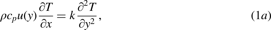
The equation that describes the temperature field T(x,y) of a fluid flowing between two parallel plates in steady state and not considering axial conduction is given by the thermal energy conservation equation

ρ c_{p} u (y) \frac{\partial T}{\partial x} = k \frac{\partial^{2} T}{\partial y^{2}},

(1a)

With boundary and initial conditions

T (0, y) = T_{0} (y), \frac{\partial T}{\partial y} (x, 0) = 0, - k {\frac{\partial T}{\partial y} |}_{y = H} = h_{e} (T (x, H) - T_{\infty}),

(1b)

where

ρ

and

c_{p}

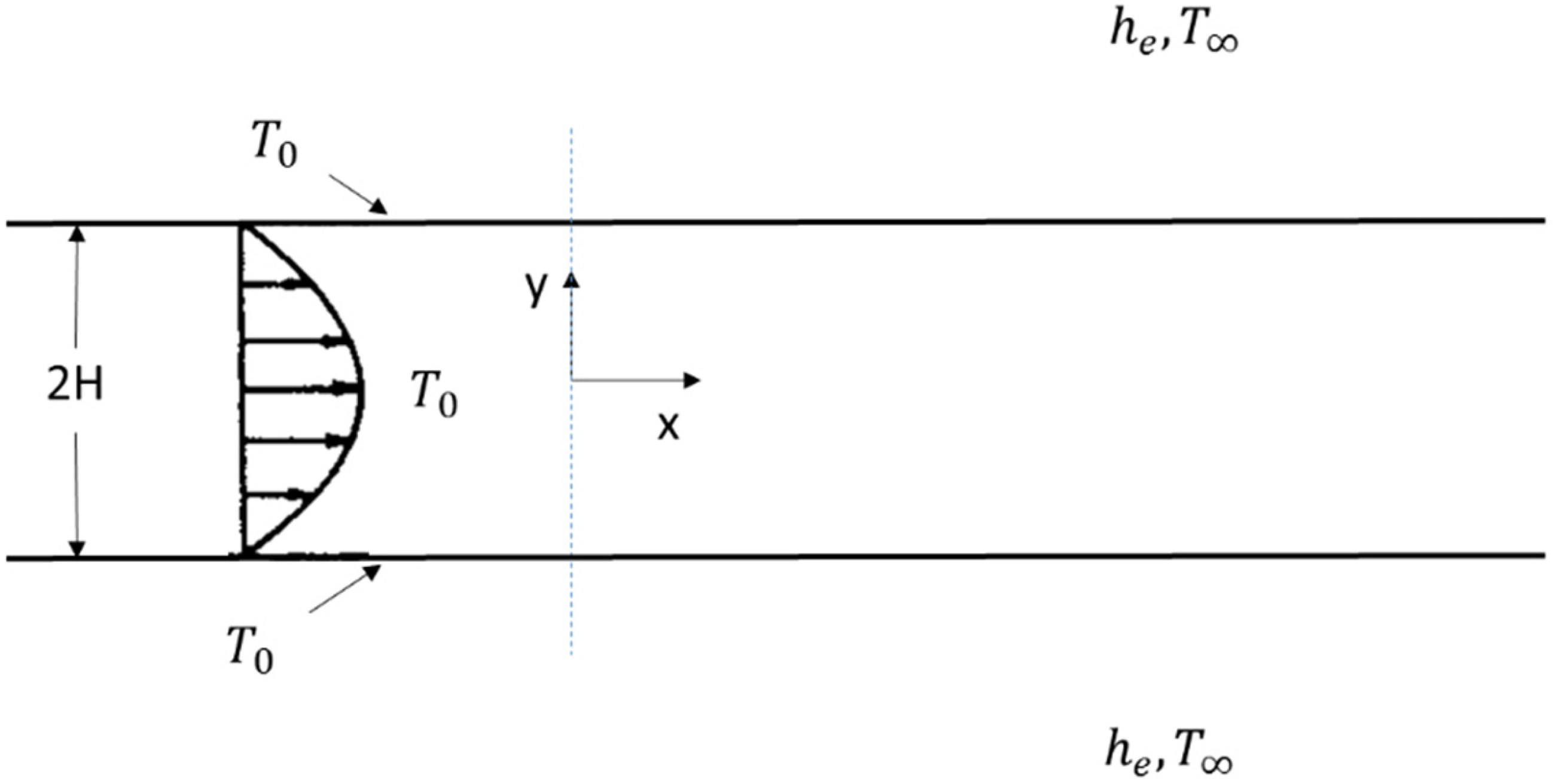
are the density and the specific heat coefficient of the fluid, k is the thermal conductivity and

u (y)

is the velocity profile (parabolic profile). Figure 2 shows a geometric diagram of the problem.

Figure 2.

Laminar flow developed between parallel plates.

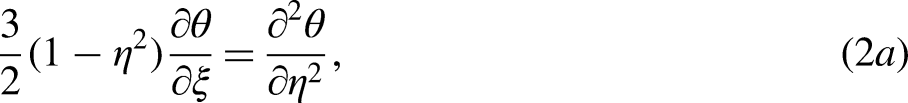
Defining dimensionless coordinates $ξ = x / (R e P r H)$ , $η = y / H$ and $θ = \frac{T - T_{\infty}}{T_{0} - T_{\infty}}$ , equation (1) is given by

\frac{3}{2} (1 - η^{2}) \frac{\partial θ}{\partial ξ} = \frac{\partial^{2} θ}{\partial η^{2}},

(2a)

with boundary and initial conditions

θ (0, η) = θ_{0} (η) = 1 \frac{\partial θ}{\partial η} (ξ, 0) = 0 - {\frac{\partial θ}{\partial η} |}_{η = 1} = Bi θ (ξ, 1),

(2b)

where

Bi

is the Biot number defined as

Bi = \frac{h_{e} H}{k}

h_{e}

is the external natural convection coefficient. In general, the Biot number can acquire any value

Bi \geq 0

. In the limiting case

Bi = 0

, the boundary condition of zero flow in the wall (adiabatic wall) is obtained, so it should be noted that in this case the temperature

θ

of the fluid will remain constant and equal to 1 for all values of the x coordinate, however a small value of the Bi coefficient will be enough for there to be a small amount of heat flow from the duct to the outside, in this way there will always be a sufficiently long value of the x coordinate for which the temperature has decreased by one considerable amount with respect to unity, even reaching zero asymptotically when as x tends to infinity. In this sense, the fact that the x coordinate extends indefinitely means that the problem can be classified as a singular perturbation problem. In addition, the reader should note the relevance of introducing dimensionless variables into the problem, since the differential equation obtained is independent of the physical and geometric parameters of the problem.

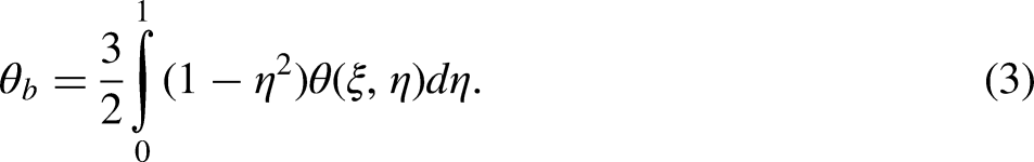
The local Nusselt number is given by $N u = - \frac{{\frac{\partial θ}{\partial η} |}_{η = 1}}{θ_{b} - θ_{w}}$ , where $θ_{b}$ is the mixing-cup temperature defined as

θ_{b} = \frac{3}{2} \int_{0}^{1} (1 - η^{2}) θ (ξ, η) d η .

(3)

The differential equation (2a) with boundary condition (2b) can be solved by classical analytical methods.^11–13 However, we can find a simple analytical solution using matching asymptotic method in the case in of small Biot numbers, this allows to find simple analytical solutions for the fluid temperature field, which can be applied in different situations.

Asymptotic analysis $(Bi = ϵ ≪ 1)$

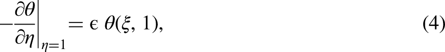
For very small values of the Biot number, the boundary condition on the wall is written as

- {\frac{\partial θ}{\partial η} |}_{η = 1} = ϵ θ (ξ, 1),

(4)

in the particular case

ϵ = 0

, it is clear that the solution of the problem is

θ (ξ, η) = 1

across the domain, in the case

0 < ϵ ≪ 1

, the temperature should vary slowly in the axial direction.

Far field $(ξ \sim ϵ^{- 1})$

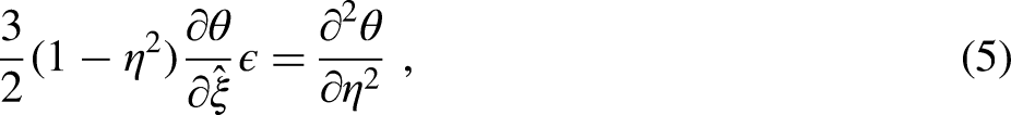
Let us consider the field of temperatures in the far field, that is, at axial distances of the order of $ξ \sim ϵ^{- 1}$ , defining the new coordinate $\hat{ξ} = ϵ ξ$ (outer coordinate), equation (1b) is transformed into

\frac{3}{2} (1 - η^{2}) \frac{\partial θ}{\partial \hat{ξ}} ϵ = \frac{\partial^{2} θ}{\partial η^{2}},

(5)

In the limit

ϵ \to 0

, equation (5) has the general solution

θ (\hat{ξ}, η) = θ_{0} (\hat{ξ}) + a (\hat{ξ}) η

, the condition of symmetry in the median plane of the channel leads to

θ (\hat{ξ}, η) = θ_{0} (\hat{ξ})

. This suggests looking for solutions of the form

θ (\hat{ξ}, η) = θ_{0} (\hat{ξ}) + ϵ θ_{1} (\hat{ξ}, η) + ϵ^{2} θ_{2} (\hat{ξ}, η) + \dots

(6)

Introducing the expansion (6) in (5), the following equation for

θ_{i} (\hat{ξ}, η)

\frac{\partial^{2} θ_{i}}{\partial η^{2}} = \frac{3}{2} (1 - η^{2}) \frac{\partial θ_{i - 1}}{\partial \hat{ξ}} i = 1, 2 \dots

(7.1)

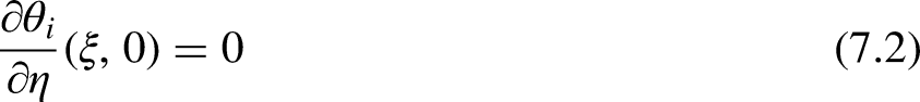
With the boundary conditions

\frac{\partial θ_{i}}{\partial η} (ξ, 0) = 0

(7.2)

- {\frac{\partial θ_{i}}{\partial η} |}_{η = 1} = θ_{i - 1} (ξ, 1)

(7.3)

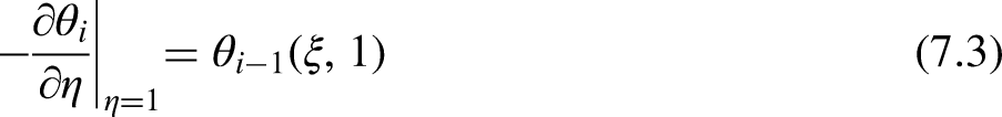
Equation (7.1) for i = 1 is given by

\frac{\partial^{2} θ_{1}}{\partial η^{2}} = \frac{3}{2} (1 - η^{2}) \frac{\partial θ_{0}}{\partial \hat{ξ}}

whose solution leads to

θ_{1} (\hat{ξ}, η) = \frac{3}{4} (η^{2} - \frac{1}{6} η^{4}) θ_{0 \hat{ξ}} (\hat{ξ}) + c_{2} (\hat{ξ})

(8)

Imposing in (8) the boundary condition (7.3), the following differential equation is obtained for

θ_{0} (\hat{ξ})

θ_{0 \hat{ξ}} (\hat{ξ}) = - θ_{0} (\hat{ξ}) .

(9)

the solution of (9) is given by

θ_{0} (\hat{ξ}) = c e^{- \hat{ξ}}

, and represents the classical lumped approximation. From (9), (8) and (6), we have

θ (\hat{ξ}, η) = c e^{- \hat{ξ}} (1 - ϵ \frac{3}{4} (η^{2} - \frac{1}{6} η^{4})) + ϵ c_{2} (\hat{ξ}) + \dots

(10)

to determine the function

c_{2} (\hat{ξ})

, we proceed to use equation (7.1) for i = 2, obtaining

\frac{\partial^{2} θ_{2}}{\partial η^{2}} = \frac{3}{2} (1 - η^{2}) (\frac{3}{4} (η^{2} - \frac{1}{6} η^{4}) θ_{0 \hat{ξ} \hat{ξ}} (\hat{ξ}) + c_{2 \hat{ξ}} (\hat{ξ}))

(11)

A first integration of this equation leads to

\frac{\partial θ_{2}}{\partial η} = \frac{3}{16} (- \frac{2}{3} η^{3} (4 c_{2 ξ} (\hat{ξ}) - 3 θ_{0 ξ \hat{ξ}} (\hat{ξ})) + (\frac{1}{7} η^{7} - \frac{7}{5} η^{5}) θ_{0 ξ \hat{ξ}} (\hat{ξ}) + 8 η c_{2 ξ} (\hat{ξ}))

(12)

Furthermore, the function

θ_{2} (\hat{ξ}, η)

must satisfy the boundary condition (7.3) for i = 2, which leads to the following differential equation for

c_{2} (\hat{ξ})

c_{2 ξ} (\hat{ξ}) = - c_{2} (\hat{ξ}) + \frac{17}{35} θ_{0} (\hat{ξ})

(13)

whose solution is given by

c_{2} (\hat{ξ}) = {\bar{c}}_{2} e^{- \hat{ξ}} + \frac{17}{35} \hat{ξ} θ_{0} (\hat{ξ})

(14)

Introducing (14) into (10), we finally obtain the following solution for the temperature field in the far field

θ (\hat{ξ}, η) = c e^{- \hat{ξ}} (1 - ϵ (\frac{3}{4} (η^{2} - \frac{1}{6} η^{4}) + \frac{{\bar{c}}_{2}}{c} + \frac{17}{35} \hat{ξ})) + \dots

(15)

The constant c and the function

{\bar{c}}_{2}

they must be determined by matching with the near field solution.

Near field $(ξ \sim O (1))$

In this region it is convenient to work with the new scaled variable

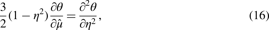
$\hat{μ} = ϵ^{- 1} \hat{ξ}$ (inner coordinate). Introducing the new scale in equation (4), we have

\frac{3}{2} (1 - η^{2}) \frac{\partial θ}{\partial \hat{μ}} = \frac{\partial^{2} θ}{\partial η^{2}},

(16)

with the boundary and initial conditions

θ (0, η) = 1 \frac{\partial θ}{\partial η} (\hat{μ}, 0) = 0 - {\frac{\partial θ}{\partial η} |}_{η = 1} = ϵ θ (\hat{μ}, 1),

(17)

In this region the temperature of the fluid varies slightly with respect to the inlet temperature, then the following expansion can be assumed for the temperature field

θ (\hat{μ}, η) = 1 + ϵ {\hat{θ}}_{1} (\hat{μ}, η) + \dots

(18)

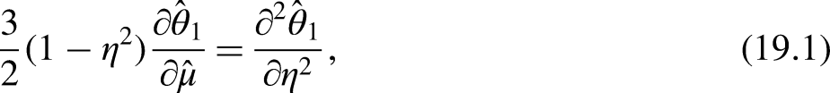
Which leads to the following differential equation for

{\hat{θ}}_{1}

\frac{3}{2} (1 - η^{2}) \frac{\partial {\hat{θ}}_{1}}{\partial \hat{μ}} = \frac{\partial^{2} {\hat{θ}}_{1}}{\partial η^{2}},

(19.1)

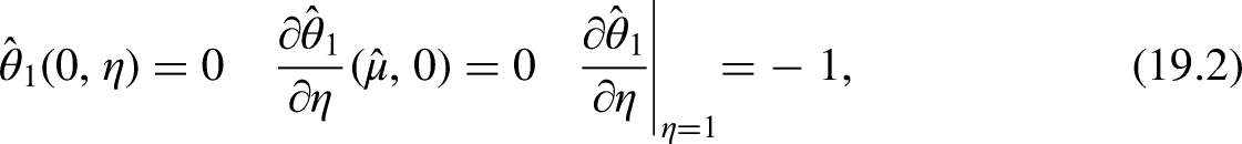
Subject to boundary and initial conditions

{\hat{θ}}_{1} (0, η) = 0 \frac{\partial {\hat{θ}}_{1}}{\partial η} (\hat{μ}, 0) = 0 {\frac{\partial {\hat{θ}}_{1}}{\partial η} |}_{η = 1} = - 1,

(19.2)

Problem (19) is well known and corresponds to the Graetz problem between parallel plates with constant heat flow in the walls,¹⁶ whose solution is given by

{\hat{θ}}_{1} (\hat{μ}, η) = - \hat{μ} - \frac{3}{4} (η^{2} - \frac{1}{6} η^{4}) + \frac{39}{280} + \sum_{n = 1}^{\infty} c_{n} Y_{n} (η) e^{- \frac{8}{3} β_{n}^{2} \hat{μ}}

(20)

Where

β_{n}

and

Y_{n} (η)

are the eigenvalues and eigenfunctions respectively of the equation

Y^{″} + β^{2} (1 - η^{2}) Y = 0

. It is important to note that the values of the coefficients

β_{n}

and functions

Y_{n} (η)

are not relevant in this study, since as will be shown in the next section, they do not contribute to the matching process.

Matching process

The region where both solutions, the near and the far field solution are valid, is given by $1 ≪ ξ ≪ ϵ^{- 1}$ , in this region the functions $\sum_{n = 1}^{\infty} c_{n} Y_{n} (η) e^{- \frac{8}{3} β_{n}^{2} \hat{μ}}$ quickly tend to zero as $e^{- \frac{8}{3} β_{n}^{2} \hat{μ}}$ . Therefore, in this region the inner solution (20) is given by

θ (\hat{μ}, η) = 1 - ϵ (\hat{μ} + \frac{3}{4} (η^{2} - \frac{1}{6} η^{4}) - \frac{39}{280})

(21)

Expressing (21) as a function of the variable

ξ

, we obtain

θ (ξ, η) = 1 - ϵ ξ - ϵ (\frac{3}{4} (η^{2} - \frac{1}{6} η^{4}) - \frac{39}{280})

(22)

On the other hand, the outer solution (15) in the matching region

1 ≪ ξ ≪ ϵ^{- 1}

, can be written as

θ (ξ, η) = c (1 - ϵ ξ + \dots) (1 - ϵ (\frac{3}{4} (η^{2} - \frac{1}{6} η^{4}) + \frac{{\bar{c}}_{2}}{c} + \frac{17}{35} ϵ ξ)) + \dots

θ (ξ, η) = c (1 - ϵ (\frac{3}{4} (η^{2} - \frac{1}{6} η^{4}) + \frac{{\bar{c}}_{2}}{c})) - c ϵ ξ + O (ϵ^{2})

(23)

Therefore, matching between equations (22) and (23) implies that

c = 1

and

{\bar{c}}_{2} = - \frac{39}{280}

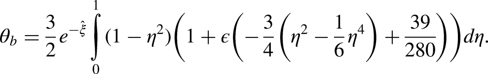
Finally we obtain the following asymptotic expression for the temperature in the far field

θ (\hat{ξ}, η) = e^{- \hat{ξ}} (1 + ϵ (- \frac{3}{4} (η^{2} - \frac{1}{6} η^{4}) + \frac{39}{280})) + O (ϵ^{2}), ϵ ≪ 1.

(24)

To evaluate the local Nusselt number we require the calculation of the mixing cup temperature and wall temperature gradient. This is done as follows

θ_{b} = \frac{3}{2} e^{- \hat{ξ}} \int_{0}^{1} (1 - η^{2}) (1 + ϵ (- \frac{3}{4} (η^{2} - \frac{1}{6} η^{4}) + \frac{39}{280})) d η .

what leads to

θ_{b} (\hat{ξ}) = e^{- \hat{ξ}}

(25)

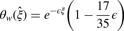
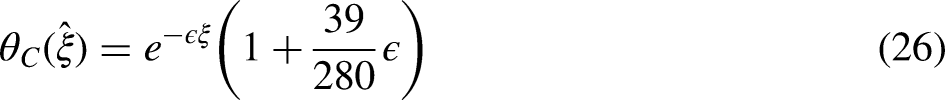
The wall temperature and the temperature in the center of the channel are given by

θ_{w} (\hat{ξ}) = e^{- ϵ ξ} (1 - \frac{17}{35} ϵ)

and

θ_{C} (\hat{ξ}) = e^{- ϵ ξ} (1 + \frac{39}{280} ϵ)

(26)

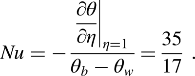
It is interesting to note that the difference between the mixing cup temperature and the wall temperature is given by

θ_{b} - θ_{w} = \frac{17}{35} ϵ e^{- \hat{ξ}}

, which leads to a constant value for the Nusselt number and independent of the Biot number

N u = - \frac{{\frac{\partial θ}{\partial η} |}_{η = 1}}{θ_{b} - θ_{w}} = \frac{35}{17} .

This value is interpreted as the asymptotic value of the Nusselt number for large values of the axial coordinate. Performing a second order analysis on

ϵ

, the following results are obtained for the wall temperature and the Nusselt number

θ_{w} (\hat{ξ}) = e^{- \hat{ξ}} + ϵ (- \frac{17}{35}) e^{- \hat{ξ}} + ϵ^{2} (\frac{701}{3252}) e^{- \hat{ξ}}

(27)

N u_{\infty} = - \frac{{\frac{\partial θ}{\partial η} |}_{η = 1}}{θ_{b} - θ_{w}} = \frac{35}{17} \frac{(1 - ϵ \frac{17}{35})}{1 - ϵ \frac{701 \cdot 35}{3252 \cdot 17}} .

(28)

Results and final comments

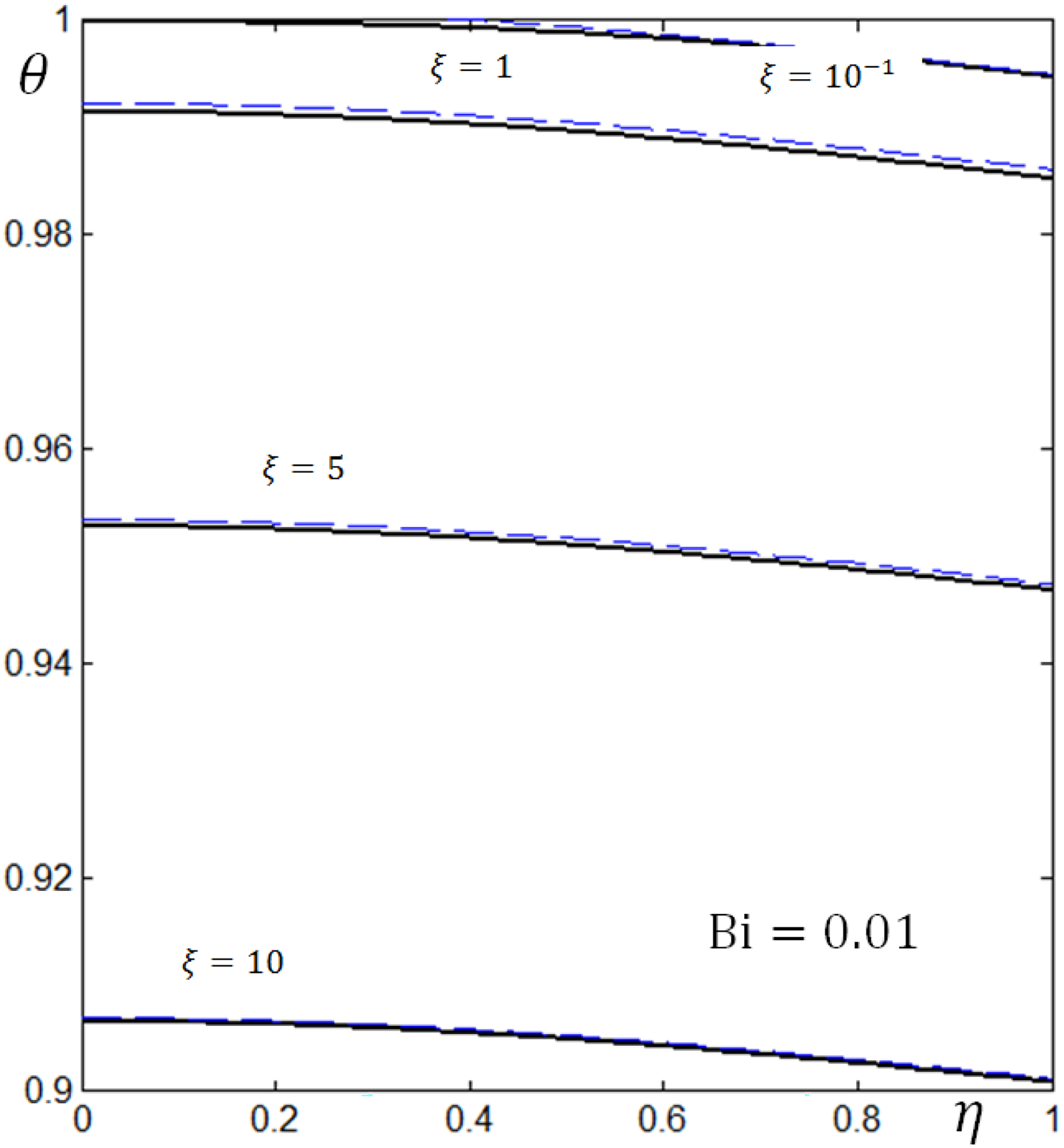
The results obtained are shown below and compared with exact numerical solutions of equations (1–2). Figure 3 shows the temperature profiles as a function of η for several values of ξ in the thermal entrance region for Biot number Bi = 0.01. The solid line represents the exact numerical solution (calculated using a semi-analytical spectral scheme)²⁸ and the segmented line represents the asymptotic solution given by equation (24).

Figure 3.

Temperature profiles as a function of η for several values of ξ in the thermal entrance region for Biot number Bi = 0.01.

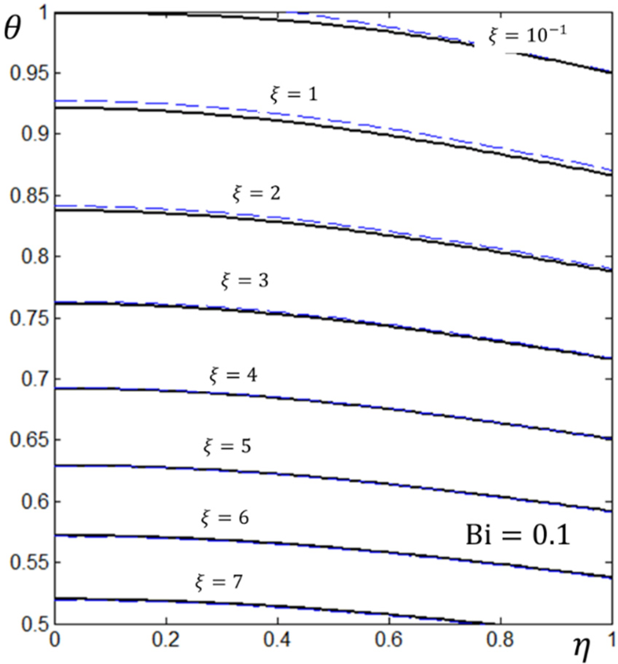
Figure 4 shows the temperature profiles as a function of η for several values of ξ in the thermal entrance region for Biot number Bi = 0.1. The solid line represents the exact numerical solution²⁸ and the segmented line represents the asymptotic solution given by equation (24).

Figure 4.

Temperature profiles as a function of η for several values of ξ in the thermal entrance region for small values of Biot number Bi = 0.1.

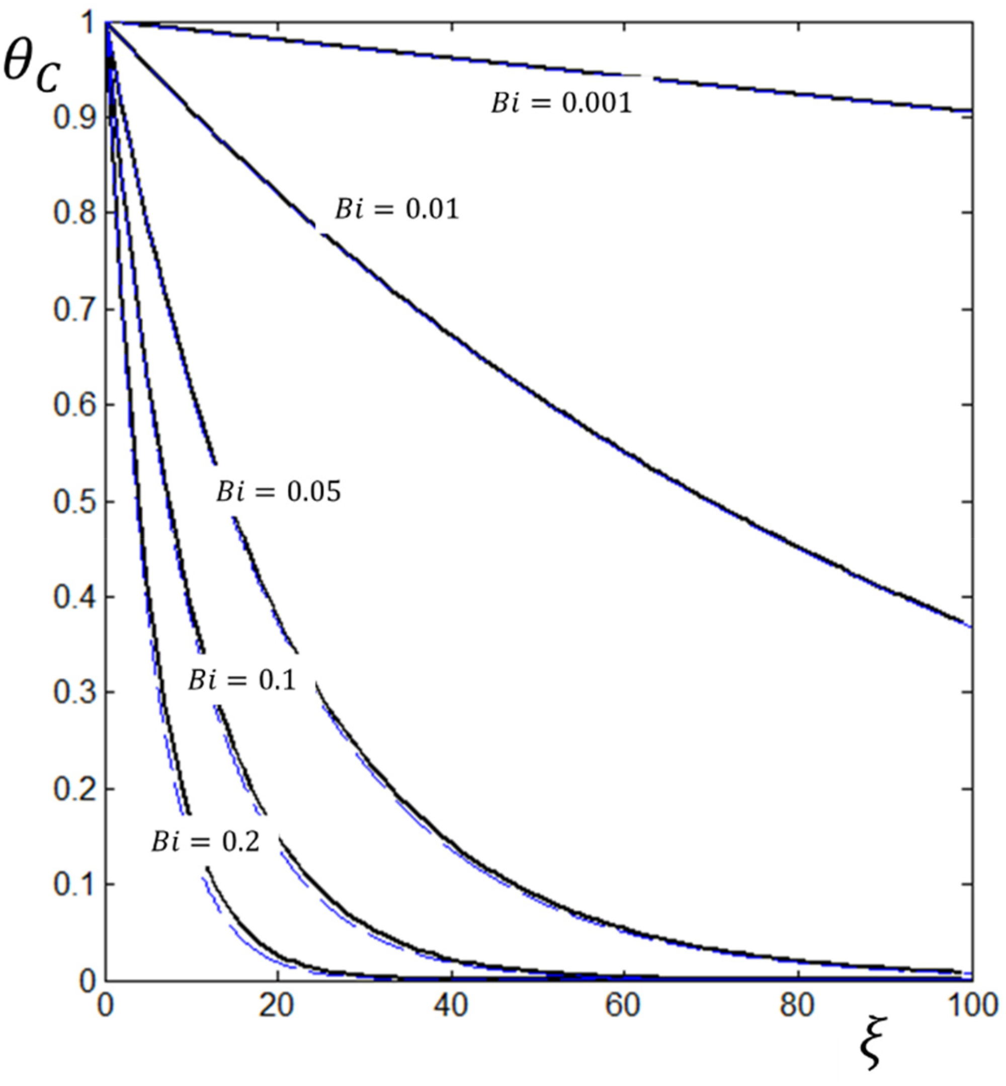
Figure 5 shows the temperature in the center of the channel as a function of ξ for several values of the Biot number. The solid line represents the exact numerical solution²⁸ and the segmented line represents the asymptotic solution given by equation (26).

Figure 5.

Temperature in the center of the channel as a function of ξ for several values of the Biot number.

These figures show that the asymptotic representation found for the far field temperature agrees very well with the exact numerical solutions, numerical tests show that the approximation works well for values of the Biot number Bi < 0.2 and $ξ > 1$ . For instance, in Figure 5, the comparison between our results and the exact solution is indistinguishable.

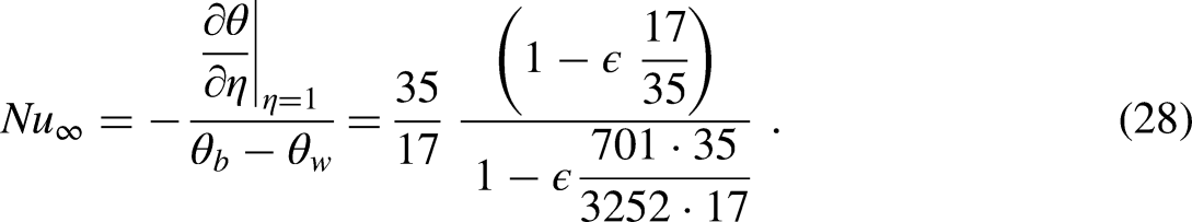
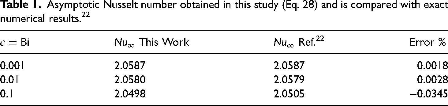
Table 1 shows the asymptotic Nusselt number obtained in this study (Eq. 28) and is compared with exact numerical results,²⁸ where you can see that the results agree quite well.

Table 1.

Asymptotic Nusselt number obtained in this study (Eq. 28) and is compared with exact numerical results.²²

$ϵ = Bi$	$N u_{\infty}$ This Work	$N u_{\infty}$ Ref.²²	Error %
0.001	2.0587	2.0587	0.0018
0.01	2.0580	2.0579	0.0028
0.1	2.0498	2.0505	−0.0345

From Table and the Figure 5, it can be seen that the approximation found for the asymptotic Nusselt number is valid (with an error less than 0.1%) for values of Bi < 0.2.

Because the method used in this paper is asymptotic in the limit $ϵ = Bi ≪ 1$ , it is clear that the range of values for the Biot number is limited. However, there are many practical cases in which this approximation is valid. For example, consider the case of a channel with a flow of water inside and air outside, in this case the external natural convection coefficient for the air is of the order $h_{e} = 5 (W / m^{2} K)$ , The thermal conductivity of water at 20 °C is k=0,598 W/m·K, then it is enough to consider a channel with a width less than 4 cm to satisfy the condition Bi < 0.2. However, if the width L of the channel wall is considered, then the overall heat transfer coefficient will be given by $\frac{1}{U} = \frac{1}{h_{e}} + \frac{L}{k_{p}}$ , where $k_{p}$ is the thermal conductivity of the wall. If the wall is made of an insulating material, this could easily result in the overall transfer coefficient being very small, thus increasing the range of applicability to different values of the half-width H of the channel.

Conclusions

The results show that the asymptotic method developed in this work provides simple analytical solutions that closely reproduce the exact numerical results quite well for low Biot numbers. The temperature of the fluid in the far field, at axial distances of the order $ξ \sim ϵ^{- 1}$ , can be approximated by the simple expression:

θ (ξ, η) = e^{- ϵ ξ} (1 + ϵ (- \frac{3}{4} (η^{2} - \frac{1}{6} η^{4}) + \frac{39}{280})) + O (ϵ^{2}), ϵ ≪ 1.

This expression improves upon the lumped approximation

θ (ξ, η) = e^{- ϵ ξ}

because it allows capturing the temperature variations in the transverse direction of the channel, which can be easily implemented in thermal engineering applications. Another notable result is the high precision provided by the analysis for the asymptotic Nusselt number, showing an error of less than 0.1% for moderately low Biot number values (Table 1). As shown in the previous chapter, the derived equation can be applied to various thermal engineering problems to estimate the heat transfer in ducts subjected to external convection where the overall external heat transfer coefficient is small, such that the Biot number satisfies the relation Bi < 0.2.

Finally, this paper may be useful for undergraduate students as an introductory example of the asymptotic matching method applied to more complex heat transfer problems.

Footnotes

Nomenclature

Pr Prandtl number

Declaration of conflicting interests

The authors declared no potential conflicts of interest with respect to the research, authorship, and/or publication of this article.

Funding

The authors received no financial support for the research, authorship, and/or publication of this article.

ORCID iD

Marco Rosales-Vera

Data availability statement

Data sharing not applicable to this article as no datasets were generated or analyzed during the current study.

References

Graetz

. Über die wärmeleitungsfähigkeit von flüssigkeiten. Ann Phys 1885; 261: 337–357.

Sellars

Tribus

Klein

. Heat transfer to laminar flow in a round tube or flat conduit—The Graetz problem extended. Trans ASME 1956; 78: 441–447.

Arpaci

. Conduction heat transfer. Boston, MA: Addison-Wesley, 1966, p. 203.

Shah

London

. Laminar flow forced convection in ducts, advances in heat transfer. New York: Academic Press, 1978.

Mansour

. Two-Dimensional heat or mass transfer in laminar flow between parallel plates: Closed-form solution. J Heat Transfer 1989; 111: 566–568.

Nickolay

Martin

. Improved approximation for the Nusselt number for hydrodynamically developed laminar flow between parallel plates. Int J Heat Mass Transfer 2000; 45: 3263–3266.

Rosales

Frederick

. Semi analytic solution to the Cartesian Graetz problem: Results for the entrance region. Int Commun Heat Mass Transfer 2004; 31: 733–740.

Prins

Mulder

Schenk

. Heat transfer in laminary flow between parallel plates. Appl Sci Res 1951; 2: 431–438.

De Bye

JVDD

Schenk

. Heat transfer in laminary flow between parallel plates. Appl Sci Res 1952; 3: 308–316.

10.

Colton

Smith

Stroeve

, et al. Laminar flow mass transfer in a flat duct with permeable walls. AIChE J 1971; 17: 773–780.

11.

Özişik

Sadeghipour

. Analytic solution for the eigenvalues and coefficients of the Graetz problem with third kind boundary condition. Int J Heat Mass Transfer 1982; 25: 736–739.

12.

Vick

Özişik

Ullrich

. Effects of axial conduction in laminar tube flow with convective boundaries. J Franklin Inst 1983; 316: 159–173.

13.

Wijeysundera

. Laminar forced convection in circular and flat ducts with wall axial conduction and external convection. Int J Heat Mass Transfer 1986; 29: 797–807.

14.

Pozzi

Lupo

. The coupling of conduction with forced convection in Graetz problems. J Heat Transfer 1990; 112: 797–806.

15.

Arici

Macia

Campo

. Finite-difference analysis of the generalized Graetz problem with heat convection boundary condition. Heat Transf Res 2020; 51: 323–328.

16.

Cess

Shaffer

. Heat transfer to laminar flow between parallel plates with a prescribed wall heat flux. Appl Sci Res 1959; 8: 339–344.

17.

Bender

Orszag

. Advanced mathematical methods for scientists and engineers. Tokyo: McGraw-Hill, 1978.

18.

Rosales-Vera

. Numerical and asymptotic analysis to the Cartesian Graetz problem with viscous dissipation. Results Appl Math 2021; 10: 100144.

19.

Acrivos

. The extended Graetz problem at low Peclet numbers. Appl Sci Res 1980; 36: 35–40.

20.

Rosales-Vera

. A Note on the Cartesian Graetz problem with viscous dissipation. Case Studies Therm Eng 2021; 28: 101391.

21.

Hudson

Bankoff

. Asymptotic solutions for the unsteady Graetz problem. Int J Heat Mass Transfer 1964; 7: 1303–1307.

22.

Sleicher

Notter

Crippen

. A solution to the turbulent Graetz problem by matched asymptotic expansions-I The case of uniform wall temperature. Chem Eng Sci 1970; 25: 845–857.

23.

Weigand

Bogenfeld

. A solution to the turbulent Graetz problem by matched asymptotic expansions for an axially rotating pipe subjected to external convection. Int J Heat Mass Transfer 2014; 78: 901–907.

24.

Rosales-Vera

. A note on Leveque's solution to the Cartesian Graetz problem with free convection. Int J Thermofluids 2022; 16: 100217.

25.

Hickman

. An asymptotic study of the Nusselt-Graetz problem—part I: large x behavior. ASME J Heat Transfer 1974; 96: 354–358.

26.

Lahjomri

Oubarra

Alemany

. Heat transfer by laminar Hartmann flow in thermal entrance region with a step change in wall temperatures: The Graetz problem extended. Int J Heat Mass Transfer 2002; 45: 1127–1148.

27.

Awad

. Heat transfer for laminar thermally developing flow in parallel-plates using the asymptotic method. In 2010 3rd international conference on thermal issues in emerging technologies theory and applications, 2010, pp. 371–387.

28.

Rosales-Vera

. Cartesian Graetz problem with boundary condition of the third kind: A semi-analytical solution. Int J Thermofluids 2022; 14: 100146.

Forced convection between parallel plates with third kind boundary condition: An asymptotic solution

Abstract

Keywords

Introduction

Analysis

Asymptotic analysis ( Bi = ϵ ≪ 1 )

Far field ( ξ ∼ ϵ − 1 )

Near field ( ξ ∼ O ( 1 ) )

Matching process

Results and final comments

Conclusions

Footnotes

Nomenclature

Pr Prandtl number

Declaration of conflicting interests

Funding

ORCID iD

Data availability statement

References

Asymptotic analysis $(Bi = ϵ ≪ 1)$

Far field $(ξ \sim ϵ^{- 1})$

Near field $(ξ \sim O (1))$