Spherical pendulum in wind: An inexpensive laboratory-scale experiment for exploring nonlinear dynamics and estimation

Abstract

This paper describes a mathematical model, estimation technique, and experiment exploring the nonlinear dynamics of a spherical pendulum subject to air drag in the presence of a steady horizontal velocity field. The pendulum’s dynamics are derived with drag as a quadratic function of the pendulum’s flow-relative velocity in both spherical and Cartesian coordinates. Numerical simulations are presented to illustrate the diverse motions that may be exhibited by the system. The model can be representative of many real-world systems that consist of an object tethered from a stationary platform in the presence of wind, or from a moving platform that induces a relative wind. The observed motion of the spherical pendulum can also be used to infer steady wind conditions. A simple experiment is described that demonstrates a pendulum-based wind sensor. A ping-pong ball is suspended on a string in the presence of an air blower and a video recording is used to measure the angular motion. The recorded measurements are then processed to infer the wind applied by the blower. Three techniques are used to compute an estimate of the wind: a static estimate based on an equilibrium assumption, a dynamic estimate that considers the instantaneous angular velocity, and an extended Kalman filtering approach. The system can serve as an instructive demonstration for students studying mechanical engineering as it provides an opportunity to discuss concepts related to damped harmonic motion, air resistance, spherical coordinates, numerical simulation, signal processing, and sensor calibration.

Keywords

spherical pendulum drag wind estimation image processing Kalman filter

Introduction

The pendulum is widely used in engineering and physics education as an example of simple harmonic motion.¹ In textbooks on engineering dynamics, it is often first treated as a concentrated point mass suspended by a massless and inextensible string oscillating in the vertical plane subject only to gravity and tension.² The pendulum is also used in a variety of laboratory experiments wherein students infer the value of gravitational acceleration and study the effects of damping.³ As noted by Nelson and Olsson,³ when using the pendulum to measure the acceleration of gravity $g$ there are a number of additional factors to consider, such as air resistance, buoyancy, added mass, and stretching of the string. More advanced discussions of the pendulum in the classroom extend to three-dimensional motion (i.e., the spherical pendulum), the swinging motion of rigid bodies (i.e., the compound pendulum), a pendulum with a vibrating support (i.e., the Kaptiza pendulum), and numerous other examples. This article investigates a spherical pendulum that is disturbed by an external source of horizontal air flow (i.e., “wind”). This type of pendulum is well-suited for engineering education as it can be relatively easily constructed with low-cost materials and provides an opportunity to reinforce or introduce concepts related to damped harmonic motion, air resistance, spherical coordinates, numerical simulation, signal processing, and sensor calibration.

Many studies have previously investigated air resistance (e.g., linear and/or quadratic drag⁴) on a pendulum. However, these have typically been studied under the assumption of still air. When an external air flow is introduced, as we shall see, its effect on the spherical pendulum model is to alter the direction and magnitude of the drag force in comparison to the drag in still air. This introduces an asymmetry in the dynamics as the pendulum swings with or against the wind. If the air flow does not vary over time, then the pendulum achieves equilibrium at an angle that is offset from the vertical. As further motivation for studying the spherical pendulum in wind, we discuss how the apparatus can be used as a simple anemometer. Our approach is conceptually similar to the educational exercise presented by Hernandez et al.⁵ wherein an optical computer mouse wheel sensor was retrofit to measure the angles of an irregularly shaped drag body and infer the wind velocity from the equilibrium angle. This article delves deeper into the equations of motion that govern this system and proposes an apparatus for experimentation that is constructed with low-cost materials that are readily available (e.g., a ping-pong ball, webcam, string, masking tape, drinking straws, and an air blower or fan). By recording videos and using image processing, the position of the pendulum bob relative to the attachment point is determined and used in subsequent analysis. This approach follows the success of prior works that have used videos for pendulum-based educational experimentation. For example, Ristano et al.⁶ used stereo cameras to characterize pendulum oscillations, and Bacon et al.⁷ recorded and analyzed videos to characterize the air drag on a swinging meter stick. Other techniques for capturing pendulum angle or timing include using smart phones⁸ and rotary motion sensors⁹. Our use of a simple spherical drag body allows comparison with well-established theoretical models and naturally prompts a discussion of concepts such as Reynolds number, turbulence, and comparison between theoretical and experimental results.

The motion of a pendulum in wind has been studied in prior work. For example, a practical motivation for analyzing the spherical pendulum in wind is to model the motion of objects tethered to a stationary platform in wind (e.g., tower cranes carrying loads in the presence of wind¹⁰), or objects tethered to a moving platform (e.g., tethered cargo being transported by helicopters¹¹). The pendulum dynamics analyzed in this paper can therefore be considered a special case of such prior works. However, our focus is on describing the dynamics of this spherical pendulum as a standalone device used as a pedagogical example for a laboratory-scale wind-sensor (anemometer). Anemometers are used in numerous applications such as measuring the atmospheric boundary in environmental science¹² and monitoring wind patterns in urban environments.¹³ Several anemometer designs have been developed that exploit various physical principles which present an opportunity to discuss with students:

Hot-wire¹⁴ anemometers rely on convective cooling effects on a temperature-sensitive resistive material.¹⁵

Sonic anemometers¹⁶ are based on the principle of air flow perturbing the speed of sound travel time between an acoustic transmitter and receiver and measuring the resulting phase shift or delay of a pulse train.¹⁷

Cup anemometers¹⁸ capture wind along several paddles or cups and convert this into rotational motion that can be measured with encoders or other means and correlated with wind speed.¹⁸

Multi-hole pressure probes¹⁹ obtain three components of flow velocity by comparing differential, static, and total pressures (according to Bernoulli’s equation) measured by pressure transducers and using a look-up-table obtained from wind tunnel calibration.²⁰

Drag body devices²¹ typically use a sphere (or other object with a well identified drag model²²) mounted on a rigid support. The deflection of the support under the influence of a wind-induced aerodynamic force is measured (e.g., using strain gauges,^21,23 lasers with position-sensitive detectors (PSDs) to measure displacement²⁴, or other techniques.^25,26)

The design proposed in this paper is most closely associated with the drag body devices mentioned above. Spheres used for this purpose simplify analysis due to their symmetry and because their drag coefficient (as a function of Reynolds number) has been well-documented.^22,27

Three wind estimation techniques are proposed that rely on angular data of the pendulum model. The first two methods are the simplest and rely on either (1) an equilibrium assumption giving a closed-form wind estimate equation, or (2) a numerical approach that considers the non-equilibrium dynamics. Lastly, this paper also describes the use of Kalman filtering for estimating the magnitude of a steady wind. While Kalman filtering is a more advanced topic it can potentially be incorporated into a lab or classroom demonstration related to mechatronics, control, or signal processing, similar to the popular experiment involving control and system identification of an inverted pendulum.^28–30

In summary, the contributions of this paper are: (1) a teaching method that uses an analytical model of the equations of motion of the spherical pendulum in wind derived in both spherical and Cartesian coordinates, (2) three methods to infer the steady wind components from a time-history of pendulum angles, and (3) an apparatus and experimental comparison that can be used for classroom demonstration.

The remainder of the paper is organized as follows. First, a model of the dynamics of the spherical pendulum in wind is formulated. Next, numerical simulations are presented and an alternate set of singularity-free equations are derived. Several approaches to estimate the components of the wind speed by observing the pendulum’s motion are then presented. Next, an experimental apparatus and demonstration is described that illustrates the wind estimation approach. Finally, the paper is concluded and future work is described.

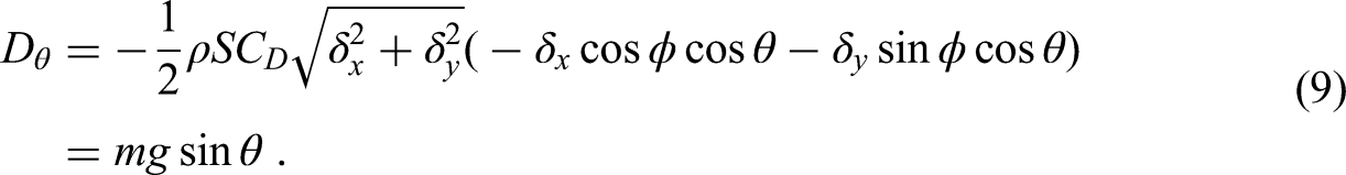
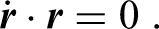
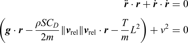
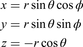
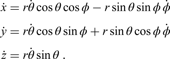
Analytical model

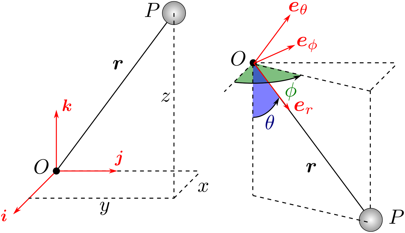
Consider a spherical pendulum with a bob of mass $m$ attached at point $P$ to the end of a massless and inextensible taut string fixed at the origin point $O$ . The dynamics of the pendulum are modeled in a spherical reference frame ${O, e_{r}, e_{ϕ}, e_{θ}}$ that has the ortho-normal unit vectors $e_{r}$ , $e_{ϕ}$ , and $e_{θ}$ forming a right-handed system as shown in Figure 1.

Figure 1.

Left: Cartesian coordinate system. Right: Spherical coordinate system.

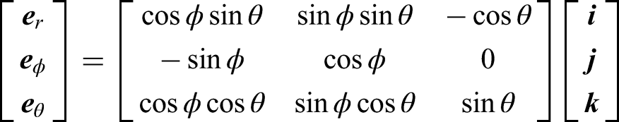
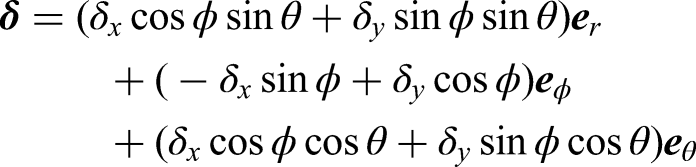
The position of a particle is described in the spherical frame by the coordinates $(r, ϕ, θ)$ where $r$ is the distance of the particle $P$ from the origin $O$ , $θ$ is the polar angle that measures the deflection of point $P$ from the vertical (down) direction, and $ϕ$ is the angle measured in the horizontal plane positive counter-clockwise when viewed from above. In this convention, the stable resting equilibrium point is at $θ = 0$ . The standard kinematics of a particle $P$ are described in the spherical frame according to Greenwood³¹:

r = r e_{r}

(1)

\dot{r} = \dot{r} e_{r} + r \dot{ϕ} \sin θ e_{ϕ} + r \dot{θ} e_{θ}

(2)

\begin{aligned} \ddot{r} & = (\ddot{r} - r {\dot{ϕ}}^{2} \sin^{2} θ - r {\dot{θ}}^{2}) e_{r} \\ + (r \ddot{ϕ} \sin θ + 2 \dot{r} \dot{ϕ} \sin θ + 2 r \dot{ϕ} \dot{θ} \cos θ) e_{ϕ} \\ + (r \ddot{θ} + 2 \dot{r} \dot{θ} - r {\dot{ϕ}}^{2} \sin θ \cos θ) e_{θ}, \end{aligned}

(3)

where

r

\dot{r}

, and

\ddot{r}

are the inertial position, velocity, and acceleration vectors, respectively. Under the assumptions that the string is taut,

r = L

so that

\dot{r} = \ddot{r} = 0

and (1)–(3) simplify as

\begin{aligned} r & = L e_{r} \\ \dot{r} & = L \dot{ϕ} \sin θ e_{ϕ} + L \dot{θ} e_{θ} \\ \ddot{r} & = (- L {\dot{ϕ}}^{2} \sin^{2} θ - L {\dot{θ}}^{2}) e_{r} + (L \ddot{ϕ} \sin θ + 2 L \dot{ϕ} \dot{θ} \cos θ) e_{ϕ} \\ + (L \ddot{θ} - L {\dot{ϕ}}^{2} \sin θ \cos θ) e_{θ} . \end{aligned}

Now suppose that the spherical pendulum is in the presence of a wind

δ

that is in the horizontal plane. We initially express the wind velocity in the Cartesian reference frame

{O, i, j, k}

shown in Figure 1:

δ = δ_{x} i + δ_{y} j,

where

δ_{x}

and

δ_{y}

are the wind components. The Cartesian frame and spherical frame unit vectors are related by the following rotation matrices:

\begin{aligned} [\begin{matrix} e_{r} \\ e_{ϕ} \\ e_{θ} \end{matrix}] = [\begin{matrix} \cos ϕ \sin θ & \sin ϕ \sin θ & - \cos θ \\ - \sin ϕ & \cos ϕ & 0 \\ \cos ϕ \cos θ & \sin ϕ \cos θ & \sin θ \end{matrix}] [\begin{matrix} i \\ j \\ k \end{matrix}] \end{aligned}

and

\begin{aligned} [\begin{matrix} i \\ j \\ k \end{matrix}] = [\begin{matrix} \cos ϕ \sin θ & - \sin ϕ & \cos ϕ \cos θ \\ \sin ϕ \sin θ & \cos ϕ & \sin ϕ \cos θ \\ - \cos θ & 0 & \sin θ \end{matrix}] [\begin{matrix} e_{r} \\ e_{ϕ} \\ e_{θ} \end{matrix}] . \end{aligned}

Thus, in the spherical frame,

\begin{aligned} δ & = (δ_{x} \cos ϕ \sin θ + δ_{y} \sin ϕ \sin θ) e_{r} \\ + (- δ_{x} \sin ϕ + δ_{y} \cos ϕ) e_{ϕ} \\ + (δ_{x} \cos ϕ \cos θ + δ_{y} \sin ϕ \cos θ) e_{θ} \end{aligned}

The free-body diagram of forces on the mass is shown in Figure 2.

Figure 2.

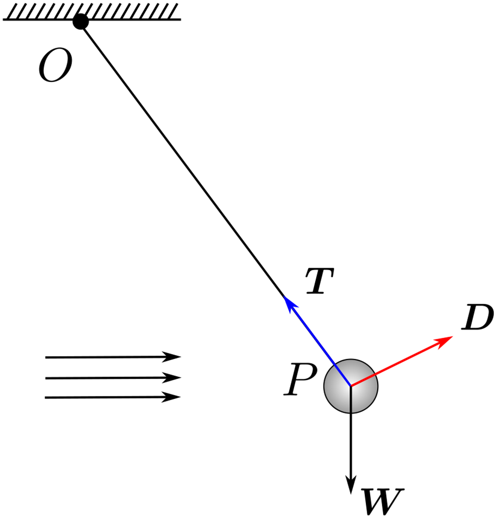
Free-body diagram of the spherical pendulum subject to a constant horizontal wind velocity.

Tension acts towards point $O$ along the length of the string, $T = - T e_{r}$ , and the weight acts directly downward

W = - m g k = - m g (- \cos θ e_{r} + \sin θ e_{θ}),

where

g

is the gravitational acceleration. Various authors have argued for either linear or quadratic damping models of drag when modeling pendulum motion in benchtop experiments.^4,9,32 This work adopts a quadratic model as it appears to provide a good fit to experimental data shown later. The drag force is

D = - \frac{1}{2} ρ S C_{D} ‖ v_{rel} ‖ v_{rel},

where

ρ

is the air density,

S

is the frontal area of the sphere,

C_{D}

is the drag coefficient, and

v_{rel} = v - δ = v_{rel, r} e_{r} + v_{rel, ϕ} e_{ϕ} + v_{rel, θ} e_{θ}

is the flow-relative velocity with components

\begin{aligned} v_{rel, r} & = - (δ_{x} \cos ϕ \sin θ + δ_{y} \sin ϕ \sin θ) \\ v_{rel, ϕ} & = L \dot{ϕ} \sin θ - (- δ_{x} \sin ϕ + δ_{y} \cos ϕ) \\ v_{rel, θ} & = L \dot{θ} - (δ_{x} \cos ϕ \cos θ + δ_{y} \sin ϕ \cos θ) \end{aligned}

and

‖ v_{rel} ‖ = \sqrt{v_{rel, r}^{2} + v_{rel, θ}^{2} + v_{rel, ϕ}^{2}}

. Even though the wind is horizontal, the relative velocity and drag may have components in all three directions of the spherical frame. The drag force is resolved as:

D = D_{r} e_{r} + D_{ϕ} e_{ϕ} + D_{θ} e_{θ} .

If the pendulum bob’s velocity exactly matches the wind velocity at a particular instant then

‖ v_{rel} ‖ = 0

and it experiences no drag. Additionally, in the presence of a constant wind, the drag is no longer symmetric as it is in the case of still air. As the pendulum swings it experiences more drag when moving against the wind than with the wind. Indeed, when the velocity of the wind surpasses the velocity of the pendulum the direction of the drag force can be aligned with the motion rather than opposed to it.

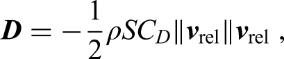
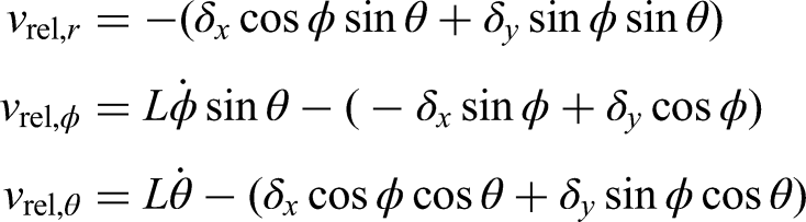
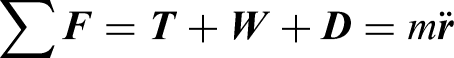
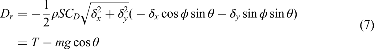
Having established all forces, the equations of motion are given by Newton’s 2nd Law:

\sum F = T + W + D = m \ddot{r}

and in component form:

- T + m g \cos θ + D_{r} = m (- L {\dot{ϕ}}^{2} \sin^{2} θ - L {\dot{θ}}^{2})

(4)

D_{ϕ} = m (L \ddot{ϕ} \sin θ + 2 L \dot{ϕ} \dot{θ} \cos θ)

(5)

- m g \sin θ + D_{θ} = m (L \ddot{θ} - L {\dot{ϕ}}^{2} \sin θ \cos θ)

(6)

The equilibrium occurs when

\dot{r} = 0

(equivalently,

\dot{ϕ} = \dot{θ} = 0

). At equilibrium the drag components are

\begin{aligned} D_{r} & = - \frac{1}{2} ρ S C_{D} \sqrt{δ_{x}^{2} + δ_{y}^{2}} (- δ_{x} \cos ϕ \sin θ - δ_{y} \sin ϕ \sin θ) \\ = T - m g \cos θ \end{aligned}

(7)

D_{ϕ} = - \frac{1}{2} ρ S C_{D} \sqrt{δ_{x}^{2} + δ_{y}^{2}} (δ_{x} \sin ϕ - δ_{y} \cos ϕ) = 0

(8)

\begin{aligned} D_{θ} & = - \frac{1}{2} ρ S C_{D} \sqrt{δ_{x}^{2} + δ_{y}^{2}} (- δ_{x} \cos ϕ \cos θ - δ_{y} \sin ϕ \cos θ) \\ = m g \sin θ . \end{aligned}

(9)

From (8) and (9) we find that the stable equilibrium angles are

ϕ = atan (\frac{δ_{y}}{δ_{x}})

(10)

θ = atan (\frac{1 / 2 ρ S C_{D} \sqrt{δ_{x}^{2} + δ_{y}^{2}} (δ_{x} \cos ϕ + δ_{y} \sin ϕ)}{m g}) .

(11)

The equilibrium azimuthal angle depends on the ratio of the horizontal speeds and the equilibrium polar angle depends on the ratio of the drag to weight force.

Numerical simulations

This section presents several illustrative simulations of the equations of motion.

Singularity-free equations of motion

One of the challenges with simulating the system above is that a singularity exists at $θ = 0$ where the azimuthal angle becomes undefined. In a computer simulation, this manifests as $\ddot{ϕ}$ vanishing from (5) and causing numerical instabilities. One way to address this is to use an alternative set of equations, in Cartesian coordinates, that do not suffer from the singularity. Deriving the equations of motion of the pendulum in this alternative reference frame is also instructive for the student. Begin by writing Newton’s 2nd Law with the force of gravity, drag, and tension as:

m \ddot{r} = m g - \frac{1}{2} ρ S C_{D} ‖ v_{rel} ‖ v_{rel} - T r .

(12)

The position vector is constrained by the length of the pendulum (i.e., a holonomic constraint), thus

r \cdot r = L^{2} .

Differentiating once gives the intuitive result that velocity is perpendicular to position at each point,

\dot{r} \cdot r = 0 .

Differentiating again and substituting (12):

\begin{aligned} \ddot{r} \cdot r + \dot{r} \cdot \dot{r} & = 0 \\ (g \cdot r - \frac{ρ S C_{D}}{2 m} ‖ v_{rel} ‖ v_{rel} \cdot r - \frac{T}{m} L^{2}) + v^{2} & = 0 \end{aligned}

Solving for

T

T = \frac{m}{L^{2}} (v^{2} + g \cdot r - \frac{ρ S C_{D}}{2 m} ‖ v_{rel} ‖ v_{rel} \cdot r) .

(13)

Equations (12) with (13) can be readily simulated and do not suffer from any singularities. To ensure that the initial position and velocity in Cartesian coordinates is consistent with the constraints of a spherical pendulum it is useful to specify the spherical angles and rates and then perform the appropriate conversions:

\begin{aligned} x & = r \sin θ \cos ϕ \\ y & = r \sin θ \sin ϕ \\ z & = - r \cos θ \end{aligned}

and

\begin{aligned} \dot{x} & = r \dot{θ} \cos θ \cos ϕ - r \sin θ \sin ϕ \dot{ϕ} \\ \dot{y} & = r \dot{θ} \cos θ \sin ϕ + r \sin θ \cos ϕ \dot{ϕ} \\ \dot{z} & = r \dot{θ} \sin θ . \end{aligned}

In the opposite direction, we can convert the Cartesian positions and rates to spherical angles and rates:

\begin{aligned} θ & = atan (- γ / z) \\ ϕ & = atan (y / x) \\ \dot{θ} & = \frac{- z (x \dot{x} + y \dot{y}) + γ^{2} \dot{z}}{γ L} \\ \dot{ϕ} & = \frac{x \dot{y} - y \dot{x}}{x^{2} + y^{2}} \end{aligned}

where

γ = \sqrt{x^{2} + y^{2}}

Illustrative simulations

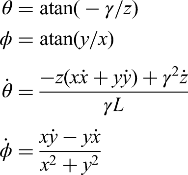
A set of four numerical simulation of the spherical pendulum in a steady wind are shown in Figures 3 –6 .

Figure 3.

$ϕ (t_{0}) = 5 π / 4$ , $\dot{ϕ} (t_{0}) = 0$ , $θ (t_{0}) = π / 2$ , $\dot{θ} (t_{0}) = 0$ at time $t_{0} = 0$ with $δ_{x} = 5$ m/s and $δ_{y} = 0$ .

Figure 4.

$ϕ (t_{0}) = 5 π / 4$ , $\dot{ϕ} (t_{0}) = 0$ , $θ (t_{0}) = π / 2$ , $\dot{θ} (t_{0}) = 0$ at time $t_{0} = 0$ with $δ_{x} = 5$ m/s and $δ_{y} = 0$ .

Figure 5.

$ϕ (t_{0}) = 5 π / 4$ , $\dot{ϕ} (t_{0}) = 0$ , $θ (t_{0}) = π / 2$ , $\dot{θ} (t_{0}) = 0$ at time $t_{0} = 0$ with $δ_{x} = 10$ m/s and $δ_{y} = 5$ m/s.

Figure 6.

$ϕ (t_{0}) = 5 π / 4$ , $\dot{ϕ} (t_{0}) = 10$ , $θ (t_{0}) = π / 2$ , $\dot{θ} (t_{0}) = 0$ at time $t_{0} = 0$ with $δ_{x} = 5$ m/s and $δ_{y} = 0$ .

Figure 7.

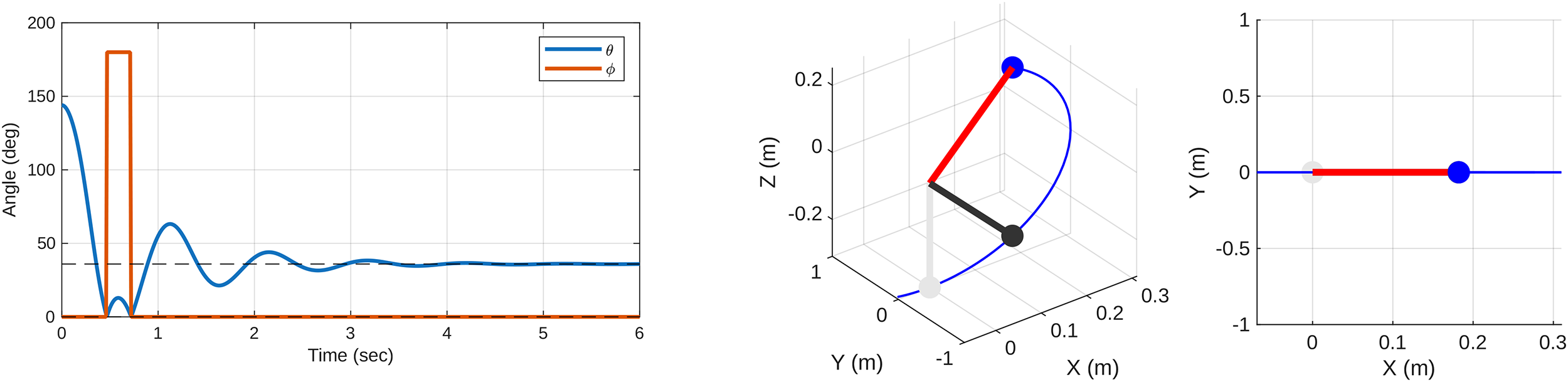
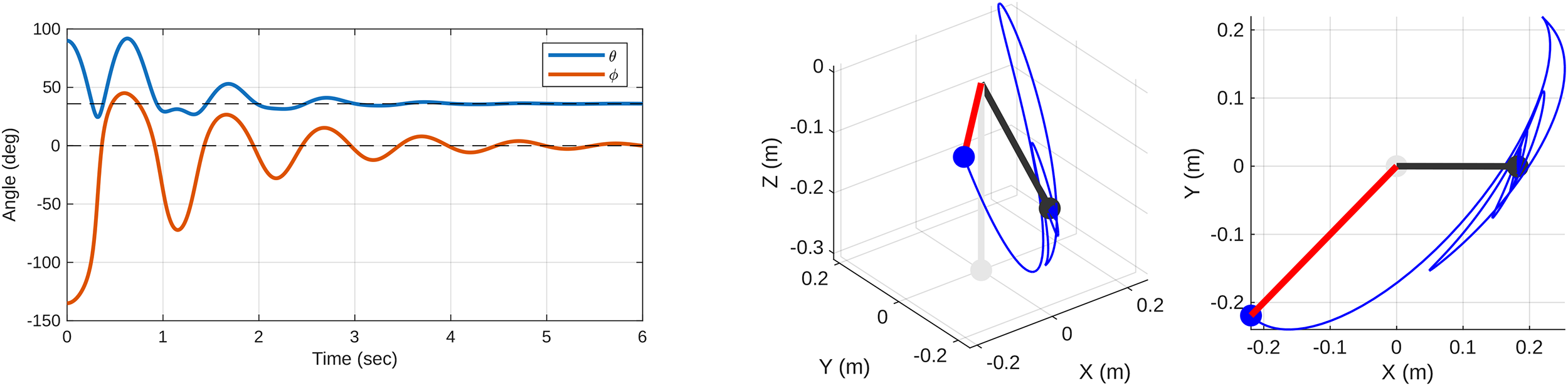
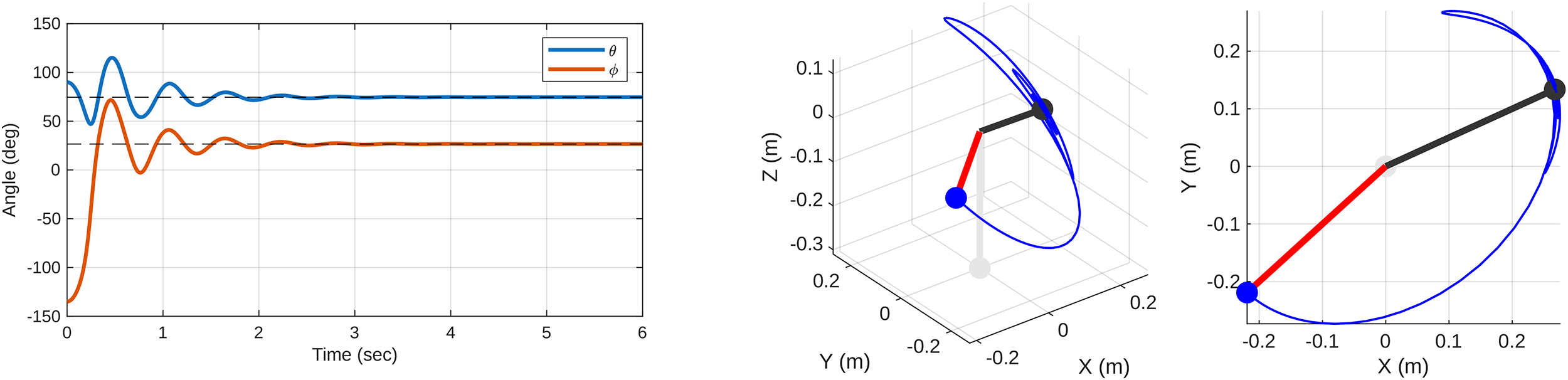
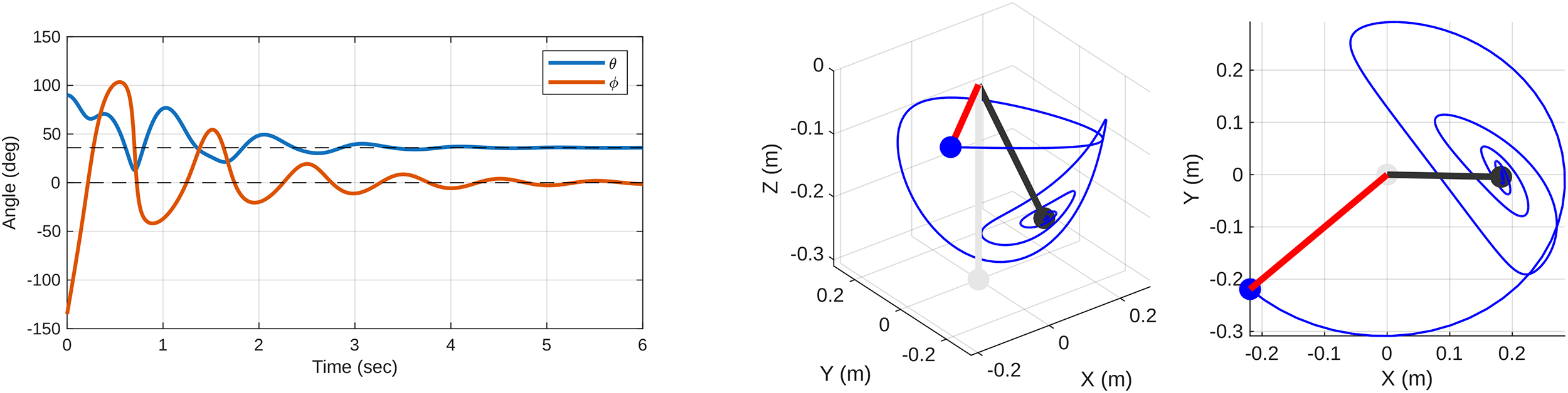
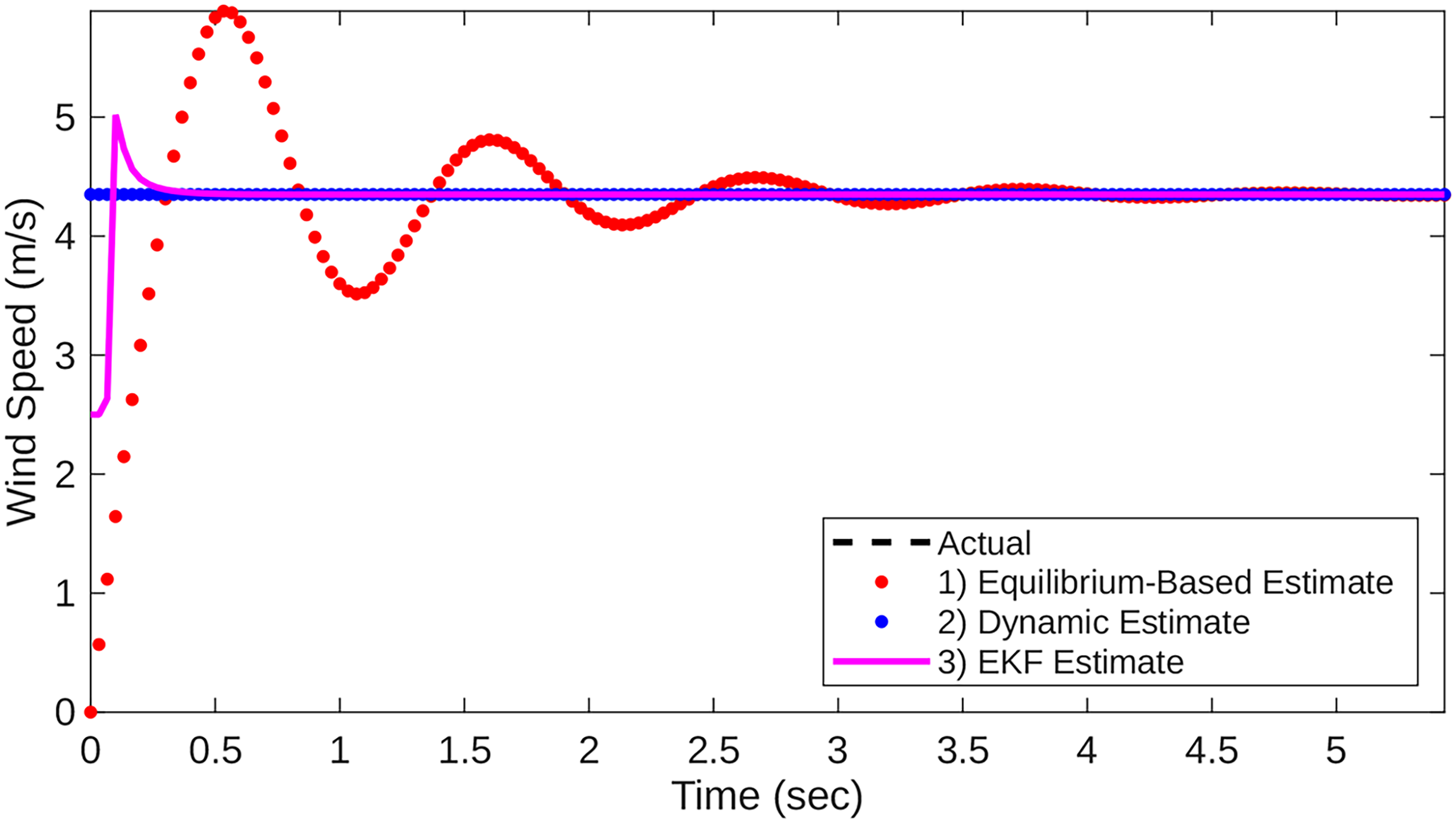
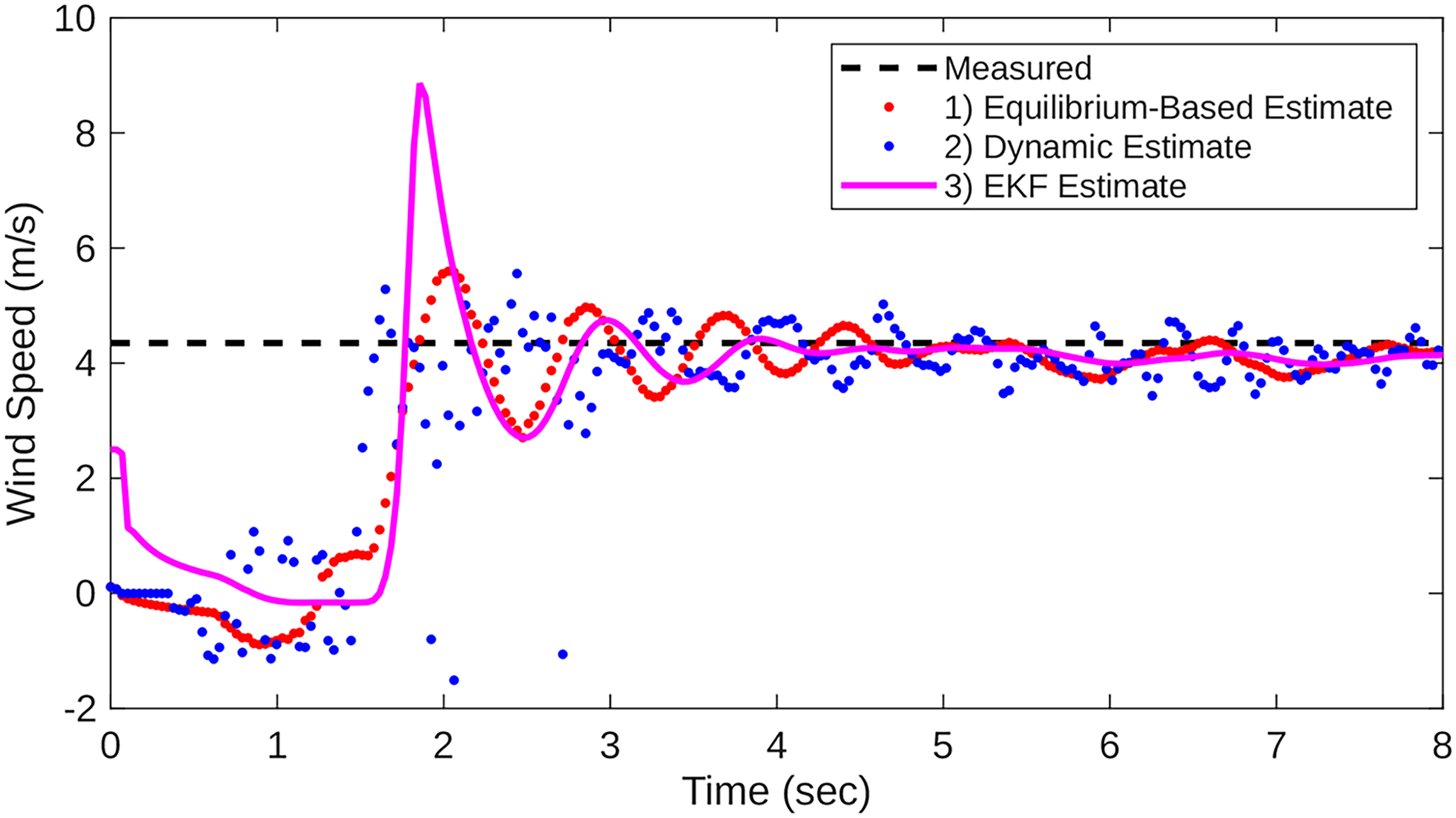
Comparison of three estimation techniques using simulated noise-free data.

The parameters of the model used in simulation (see Table 1) were chosen to be representative of the experiment to be described later.

Table 1.

Model parameters.

Parameter	Symbol	Value	Units
Mass	$m$	$2.57 \times 10^{- 3}$	kg
Length	$L$	$0.31$	m
Drag coefficient	$C_{D}$	$0.95$	–
Air density	$ρ$	$1.225$	kg/m³
Ball radius	$R$	$0.02$	m

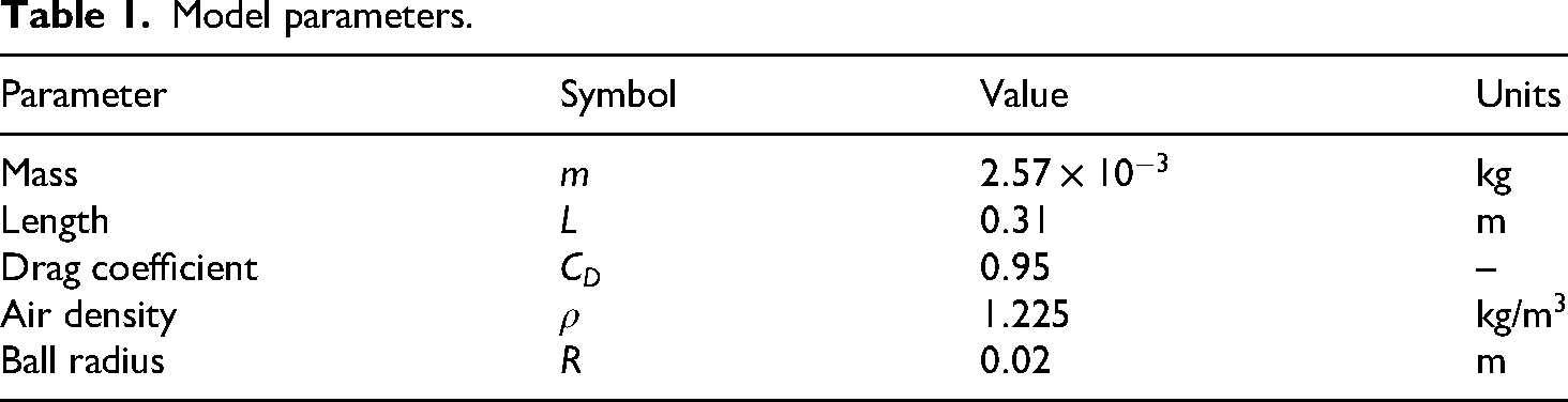
The reference area used in the drag calculation is $S = π R^{2}$ using the value of $R$ in the table above. In each of the examples in Figures 3–6 the left panel shows the time-history of the system in spherical coordinates with the dashed lines representing the equilibrium angles determined from (14) and (15). The right panels of Figures 3–6 visualize the pendulum’s path from a three-dimensional view (middle panel) and a top-down view (right-most panel). In these plots a red/blue pendulum is used to illustrate the initial configuration, a black pendulum illustrates the final position, and a gray pendulum is used to illustrate the nominal resting position (in the absence of wind). The blue curves in the right panels trace out the path of the pendulum. The axes are not equally scaled to improve the clarity of the visualization. The first three examples show the response of the pendulum from different initial positions but with no initial velocity, while the last example includes an initial azimuthal velocity. Also, the first, second, and fourth examples have a constant wind of $δ_{x} = 5$ and $δ_{y} = 0$ , while the third example has a constant wind of $δ_{x} = 10$ and $δ_{y} = 5$ . One key feature that is evident in the plots is the asymmetric nature of the oscillations about the equilibrium dashed line due to the directionality of the wind.

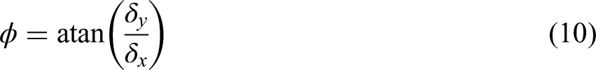
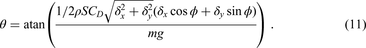
Wind estimation techniques

To determine the wind components for the case of a constant wind three approaches are considered, as described next.

Method #1: Equilibrium-Based estimate

We can rearrange the equilibrium condition (10) for 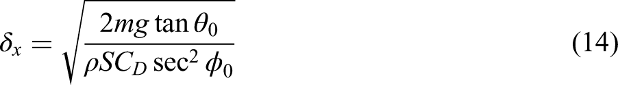$δ_{y}$ and substitute into (11) so that the wind components are determined as:

δ_{x} = \sqrt{\frac{2 m g \tan θ_{0}}{ρ S C_{D} \sec^{2} ϕ_{0}}}

(14)

δ_{y} = δ_{x} \tan ϕ_{0} .

(15)

Of course, this method can only be expected to produce good results after the pendulum has settled into a near-equilibrium configuration in a steady wind.

Moreover, a simplification occurs if the Cartesian frame is rotated so that $i$ is parallel with the wind and the pendulum’s initial condition and subsequent motion is confined entirely in the $i$ - $k$ vertical plane. This case assumes that $\dot{ϕ} = 0$ , $ϕ = 0$ , $δ_{y} = 0$ and thus the flow-relative components are: $v_{rel, r} = - δ_{x} \sin θ$ , $v_{rel, ϕ} = 0$ , and $v_{rel, θ} = L \dot{θ} - δ_{x} \cos θ$ . As before, the wind can be determined from the equilibrium angle:

δ_{x} = \sqrt{\frac{2 m g \tan θ_{0}}{ρ S C_{D}}} .

(16)

Method #2: Dynamic estimate

If instead we consider the pendulum at a non-equilibrium point then (4)–(6) form a system of three equations with three unknown values $(T, δ_{x}, δ_{y})$ where $D_{r}, D_{θ}, D_{ϕ}$ take the form of the middle terms shown in (7)–(9). These equations cannot be explicitly solved for $(δ_{x}, δ_{y})$ . However, a numerical technique may be used to solve just the pair of equations (6) and (5) for $(δ_{x}, δ_{y})$ from which the tension can be computed in (4). Again, if considering the simplified case of $ϕ = 0$ for all time then the wind can be determined by numerically solving the following equation for $δ_{x}$ :

\begin{aligned} m L \ddot{θ} = - m g \sin θ \\ - \frac{1}{2} ρ S C_{D} \sqrt{(δ_{x} \sin θ)^{2} + (L \dot{θ} - δ_{x} \cos θ)^{2}} (L \dot{θ} - δ_{x} \cos θ) . \end{aligned}

(17)

Method #3: Extended Kalman filter

Rather than only relying on the data at each particular point in time, an extended Kalman filter (EKF) recursively compresses all past information into the current estimate of the state that is more robust to measurement and modeling errors or noise. The predecessor of the EKF, the Kalman filter (KF), was invented in 1960 by engineer Rudolf E. Kalman³³ to recursively estimate the state of a linear dynamical system under Gaussian measurement and process noise. The key idea is that the state of a dynamical system is represented by a Gaussian random vector with a mean and covariance that can be updated recursively as new measurements are obtained. The KF assumes knowledge of how much the dynamic process may vary due to inherent process noise and how much the measurement of the process may vary due to sensor noise (represented as covariance matrices). When a new measurement is obtained, a prediction of the state/measurement is compared to the actual obtained measurement and the estimate of the system state is produced that combines both sources of information (sensor and prediction) in an optimal (least-square error) way. By including knowledge of the underlying physics the estimate obtained is provably optimal and generally superior to an estimate based on traditional filtering (e.g., a low-pass filter). The KF was later extended to handle dynamics that are nonlinear, leading to the “extended” KF. A variant of the EKF was used in the Apollo lunar module’s guidance system. The history surrounding the use of the EKF in the Apollo program can be of interest to students.

In the problem of this paper, the pendulum’s dynamics evolve in continuous time while the measurements are regularly spaced in discrete time. Hence, a sampled-data EKF is used (refer to Simon³⁴ for more details). We again restrict our analysis here to the case where the motion is purely in the $i$ - $k$ vertical plane as described above. Begin by writing the dynamics as a system of first-order differential equations. Let $x = [θ, \dot{θ}, δ_{x}]^{T} = [x_{1}, x_{2}, x_{3}]^{T}$ denote the state vector. The continuous system dynamics are then:

{\dot{x}}_{1} = x_{2},

(18)

{\dot{x}}_{2} = - \frac{g}{L} \sin θ - \frac{1}{2 m L} ρ S C_{D} ζ \sqrt{(x_{3} \sin x_{1})^{2} + ζ^{2}},

(19)

{\dot{x}}_{3} = 0,

(20)

where

ζ = L x_{2} - x_{3} \cos x_{1}

. The first equation comes from the definition of the state vector, the second equation is a rearranged form of (17), and the third equation is an assumption that the wind is constant or slowly varying

({\dot{δ}}_{x} = 0)

There are many references that provide step-by-step procedures for designing a sampled-data EKF (e.g., see Simon³⁴). We omit repeating these descriptions here and focus on providing the Jacobian of (18)–(20) which is required for the linearization step of the EKF. The Jacobian is

J = [\begin{matrix} 0 & 1 & 0 \\ J_{21} & J_{22} & J_{23} \\ 0 & 0 & 1 \end{matrix}]

where

\begin{aligned} J_{21} & = - \frac{2 g \cos x_{1} + \frac{x_{3} k \sin (θ) (x_{3}^{2} + 2 L^{2} x_{2}^{2} - 3 x_{3} L x_{2} \cos x_{1})}{\sqrt{α}}}{2 L} \\ J_{22} & = - \frac{k (x_{3}^{2} \cos (2 x_{1}) + 3 x_{3}^{2} + 4 L^{2} x_{2}^{2} - 8 x_{3} L x_{2} \cos x_{1})}{4 \sqrt{α}} \\ J_{23} & = \frac{k (4 \cos x_{1} (x_{3}^{2} + L^{2} x_{2}^{2}) - x_{3} L x_{2} (3 \cos (2 x_{1}) + 5))}{4 \sqrt{α} L} \end{aligned}

and

k = C_{D} ρ S / m

and

α = x_{3}^{2} + L^{2} x_{2}^{2} - 2 L x_{3} x_{2} \cos x_{1}

. In our implementation of the EKF it is assumed that only the angle of the pendulum is measured, and the measurement equation is therefore:

y = x_{1} + v

(21)

where

v

is zero-mean Gaussian measurement noise with variance

σ_{v}^{2}

. The measurement noise variance is set equal to

σ_{v}^{2} = 1 \deg^{2}

in simulations and experimental analysis.

Simulation example

The three estimation techniques are compared in Figure 7 for a simulation that begins with the pendulum hanging downward at rest in the presence of a wind of 4.35 m/s. The Kalman filter is initialized hanging with an estimate of 2.5 m/s. In this example, the equilibrium point estimate varies as the pendulum oscillates but begins to settle around the actual value after a few seconds. The dynamic point estimate, which considers perfect knowledge of the angular rate, continuously estimates the correct value of the wind. The EKF approach requires about half a second to converge.

Experimental demonstration

Apparatus

A laboratory spherical pendulum was developed that consisted of a standard ping-pong ball (see left panel of Figure 8) tied on a string (a fishing line) and suspended from a wooden plank. The connection point was secured at the edge of the plank with masking tape. The source of wind was a custom-made blower that was built from an 11 inch drone propeller, brushless motor, and electronic speed controller (ESC). The ESC was powered by a 21 V DC power supply and connected to an Arduino control board. A laptop was used to set the throttle percentage to the ESC. As can be seen in Figure 8, the propeller was mounted inside of a duct which contained a large number of drinking straws that are glued together. Forcing the air to pass through the straws helps remove rotational components of the air flow to produce more consistent and uniform flow for experimentation (similar “flow straighteners” are often used in the design of wind tunnels).

Figure 8.

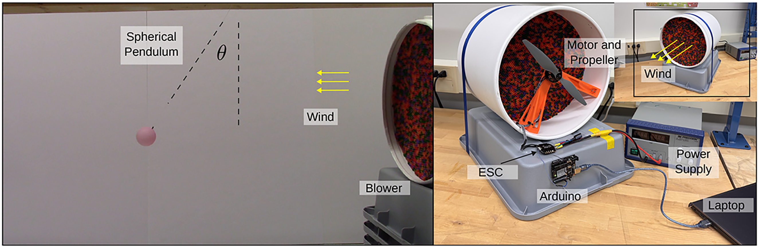
The experimental setup included a drag body spherical pendulum, webcam, and blower.

In principle, this custom propeller and flow straightener setup can be replaced by any sufficiently powerful fan or blower to reproduce the experiment. A rigidly mounted webcam recorded the motion of the pendulum in response to an applied wind. The parameters of Table 1 were assumed. The density was assumed to be standard sea-level density and the mass, string length, and sphere radius could be measured directly. Anticipating flow speeds of around 5 m/s the Reynolds number is approximately 13,300. The drag coefficient (of the ping-pong ball sphere only) based on this Reynolds number²⁷ is $C_{D} = 0.4241$ and is relatively constant in this speed regime.

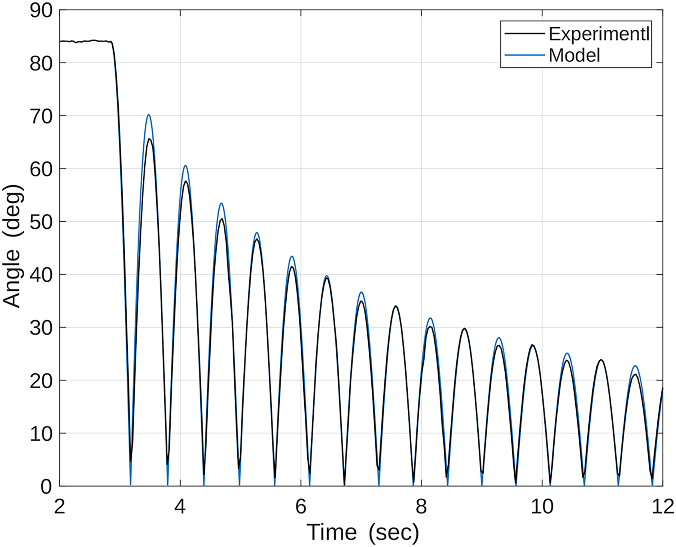
The simulated motion of the pendulum with the theoretical drag coefficient above did not produce a good match with experimental data. Thus, it was manually tuned to provide a better fit. The fit was conducted by comparing the output of the simulation to an experiment in which the ball was released from rest at an angle of about 84 degrees. The results are shown in Figure 9. A value of $C_{D} = 0.95$ produced a reasonable match to the data in both amplitude and period of the oscillation for over 40 seconds. This higher value of the drag coefficient might be attributed to the additional drag due to the string by which the ping-pong ball is suspended and the drag due to the eye hook used to secure the string to the ball. Indeed, prior work has shown in similar pendulum experiments that the drag of a fishing line can be equal to or greater than the drag on a bob³² and the thickness of the string has a significant effect on the damping coefficient.³⁵ Nonetheless, a more comprehensive characterization of drag build-up from various sources on the apparatus is merited in future work.

Figure 9.

Experiment and model comparison for the pendulum released from rest at an angle of about 84 deg. in the absence of wind.

An interesting asymmetry was observed in amplitude of the experimental data (i.e., the amplitude reduces and then increases with every oscillation). This suggests unaccounted for energy storage in the system. The fishing line used was previously reeled on a spool and without the weight of the ball it had a moderate curve and springiness. It is possible that the string holding the ping-pong ball behaves like a leaf spring that asymmetrically stores and releases potential energy. The interaction of the adhesive of the masking tape or a slight angular offset in how it was secured could have also played a role as the string was clamped by the tape rather than pinned to a spherical free joint.

Data collection and image processing

Data was recorded by the webcam at 30 Hz and was then saved as a series of images corresponding to each frame (1920 x 1080 pixels). A color mask based on a range of values similar to the pink hue of the ping-pong ball was created and applied to the images, resulting in a new binary image. The binary image was further refined by removing all connected components in the image that have fewer than a threshold number of pixels. Next, a “hole filling” operation was performed to address the reflection/glare on the ball and produce a nearly circular image. Lastly, the circular Hough transform was used to determine the center of the circle. 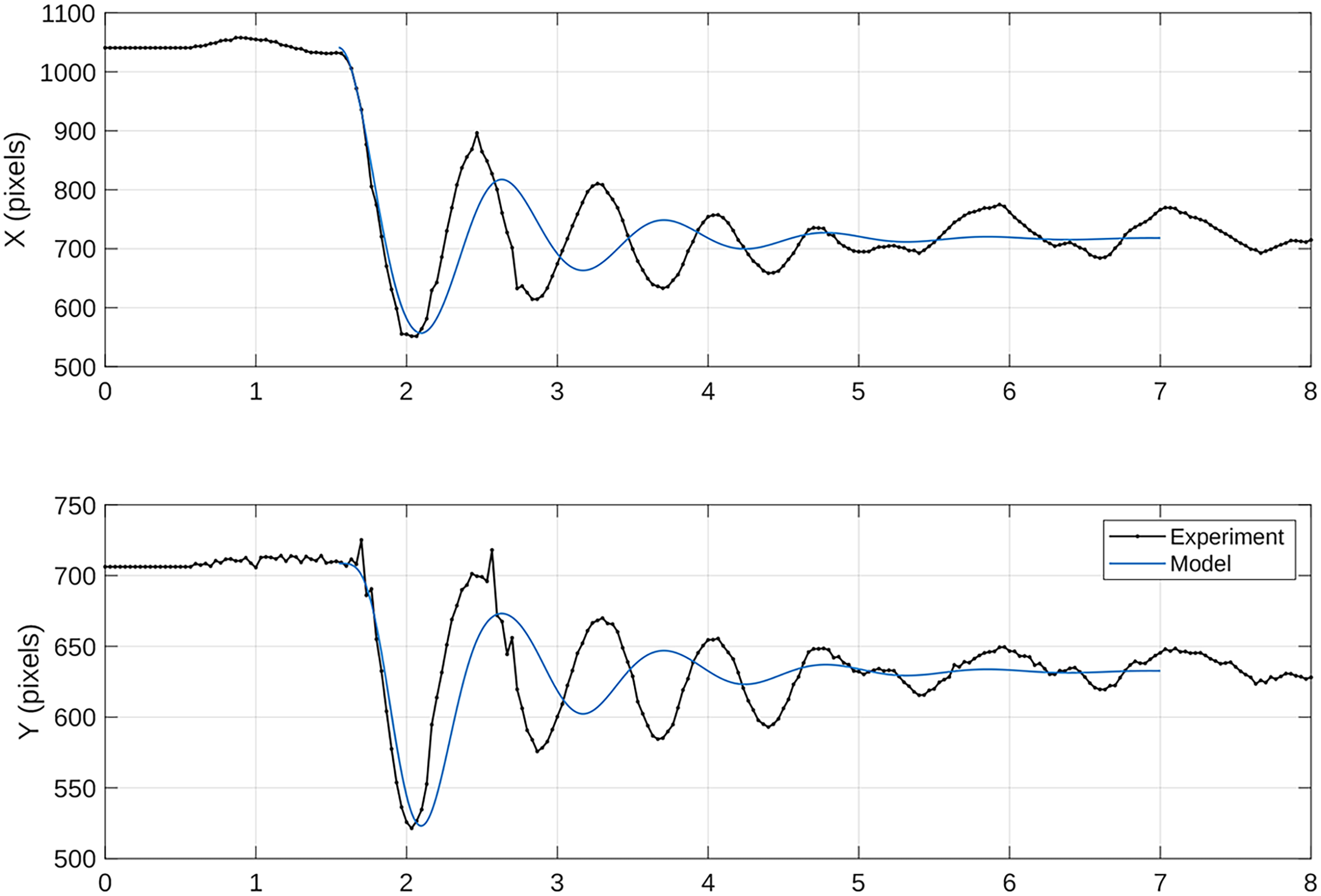The MATLAB functions used in this procedure include: rgb2hsv, bwareaopen, imfill, bwboundaries, and imfindcircles. The output of the circle-finding algorithm is a set of locations for the image pixel locations detected in each image. The resulting dataset is shown in Figure 10 along with a simulation using the parameters of Table 1.

Figure 10.

Time history of image pixel data collected.

The videos being processed all began with the ball hanging at rest. Once the image pixels were obtained, the first few seconds were averaged to establish this nominal (downward-hanging) position of the center of the ball. Next, the location of the hinge point of the string in pixel units (directly above the nominal position) was determined by inspection of the image and marked. From these reference points the angle of the pendulum could be computed. To compute the angular rate and angular acceleration a basic finite (forward) differencing scheme was applied. A second order low pass filter was applied to the angular rate and angular acceleration data to improve the smoothness of the results. The resulting angular data is shown in Figure 11 with an overlay of simulated data. The simulated data uses the model parameters of Table 1 with an assumed wind speed of 4.15 m/s. The experimental data and the simulated model exhibit some discrepancy that appears as a change in damping and shorter period of oscillation compared to the model established in the absence of wind (Figure 9). Possible reasons for this discrepancy are discussed later in this article.

Figure 11.

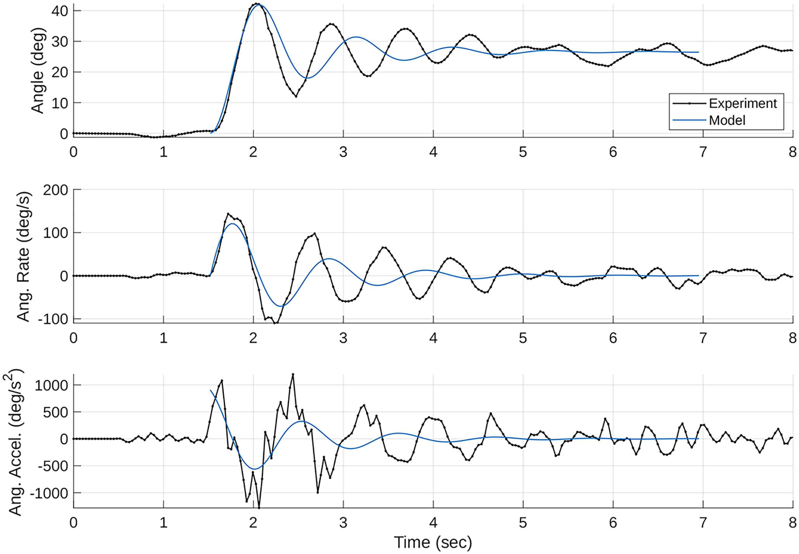
Time history of inferred angular data from experiment.

Wind estimation: Experimental evaluation

A series of experiments were performed wherein the ping-pong ball initially began at rest and subsequently was perturbed by starting the blower. The experiments were around a minute in length and the air blower was set to various throttle settings (ranging from 20% to 70% in 10% increments). Independently, prior to the experiment, a low-cost handheld anemometer (Model: Btmeter BT $-$ 100 digital vane anemometer) was used to determine the wind speed near the nominal resting position for this same set of throttle settings.

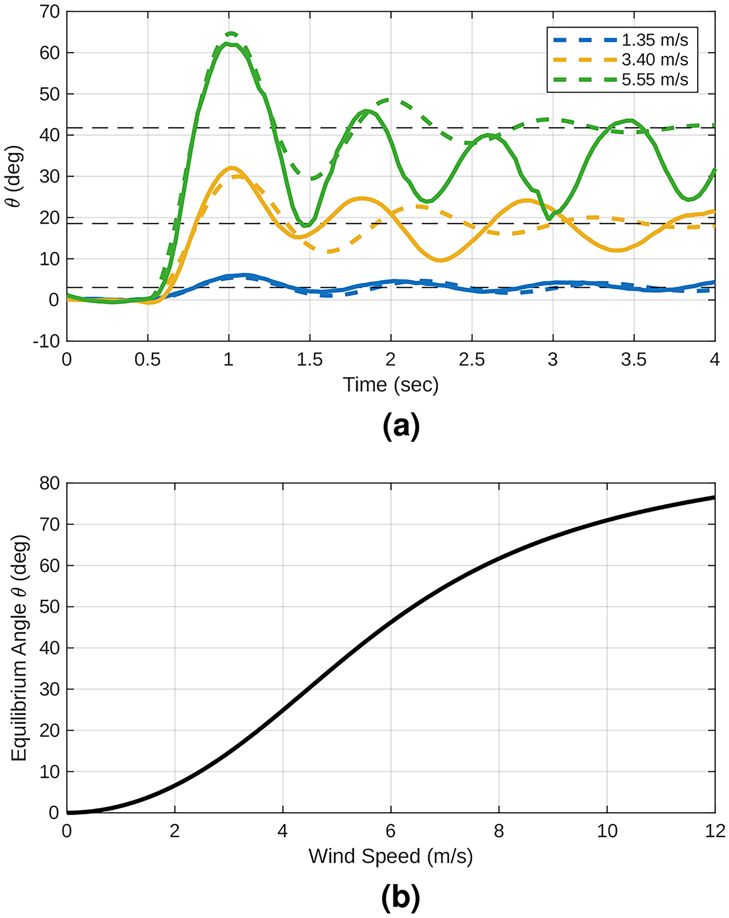
Figure 12(a) illustrates the experimental and simulated time-history response and equilibrium angle of the pendulum released from rest with wind in the $x$ direction only (i.e., the polar angle $ϕ = 0$ for all simulations). The simulations in Figure 12(a) were conducted for three representative speeds for which experimental data was available at low, medium, and high speeds (as measured with a handheld anemoemter). The horizontal dashed lines indicate the theoretical equilibrium angle for the simulated response. The colored dashed lines are the simulated response and the solid lines are the experimental data. The curve in Figure 12(b) extrapolates the theoretical equilibrium angle $θ$ for a range of speeds up to 12 m/s.

Figure 12.

Predicted response of pendulum for range of blower speeds assuming the identified model parameters in Table 1. (a) Experimental (solid lines) and simulated (dashed lines) time history of pendulum angle; (b) Predicted equilibrium angle.

The comparison in Figure 12(a) exposes some limitations of the proposed model: the magnitude of the predicted angle approximates the experimental data reasonably for the initial response (peak near 1 second), but afterwards it appears the experiment has a response with a faster natural frequency and lower damping. This is surprising as the model parameters were shown to have an excellent fit with the data in Figure 9 where the blower was off, and it is well known that a pendulum’s natural frequency depends only on its length. Moreover, for low and medium wind speeds (blue and yellow lines in Figure 12(a)) the oscillations are approximately around the predicted dashed line equilibrium, but for the green line the oscillations are around a lower angle than predicted. Further discussion of possible unmodeled effects is provided in the following section.

Figure 13 shows a comparison of the three methods used to estimate the wind over time for the case of 40% throttle. This data is analogous to the idealized simulation of Figure 7 as it uses the same wind value and initial condition. The experiment data from this trial is shown in Figure 11.

Figure 13.

Comparison of three estimation techniques using experimental data with 50% throttle.

During the initial start-up phase from 0–3 seconds the EKF is converging from its initial condition. Once converged, the EKF performs well and holds a relatively steady value with some small oscillations. Unlike the ideal (noise-free) case, the EKF estimate performs better than the dynamic estimate when using real (noisy) data. The dynamic estimate is particularly susceptible to errors in angular velocity, as illustrated by several outliers visibile in Figure 13. When applying the dynamic estimation method to noisy data, the equation (17) cannot be satisfied exactly. Hence a least-square optimization is formulated using the MATLAB function fminunc. As can be observed in Figure 11, the ping-pong ball does not come to rest at an equilibrium position as the model predicts. Instead, it continuously oscillates with some amplitude around this equilibrium position. As a result, the equilibrium-based estimate also oscillates. In all three estimation cases the error is observed to decrease in time, although there is a residual oscillation on the order of a few cm/s.

The overall comparison of the three estimation techniques for different throttle settings alongside the handheld anemometer measurement is shown in Figure 14. The mean and standard deviation of the estimates from the last 10 seconds of each run was calculated and used to plot the wind estimate mean and deviation bars. The results show that the estimates match the measured speed fairly well for throttle settings of 20%, 30%, and 40% but tend to produce lower values for higher throttle settings.

Figure 14.

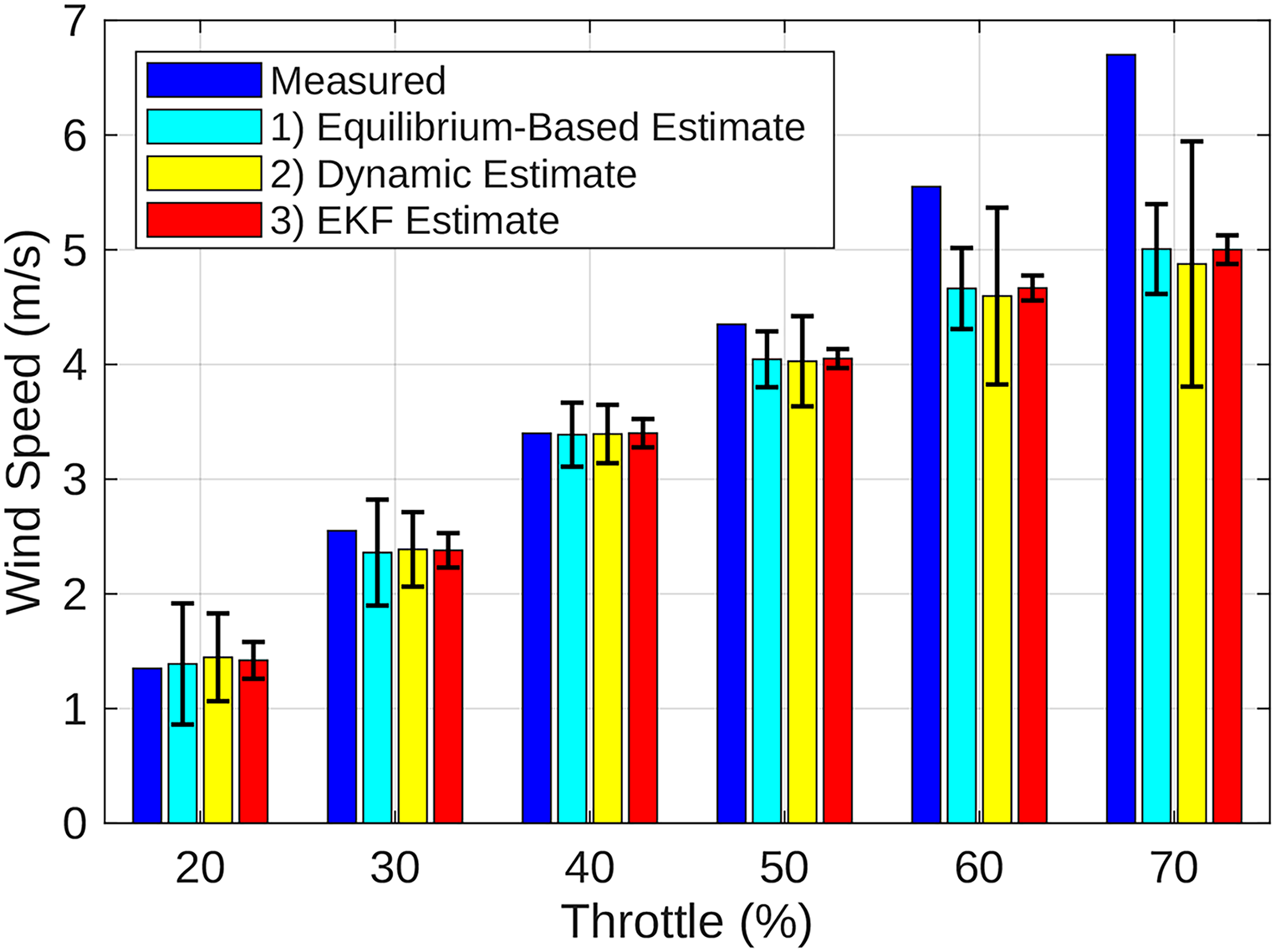
Overall comparison of wind estimates and measurement during experiments with varying throttle setting.

Among the three estimates the mean values appear fairly consistent. The EKF produces the lowest variance with a standard deviation of between 0.08–0.16 m/s for the flow speeds tested ranging from 1.35 to 6.7 m/s. This is expected since the EKF is designed to tolerate noise in measurements and produces an estimate that encodes data from a time-history of measurements, whereas the dynamic and equilibrium methods treat each data point in time independently. For low throttle settings the dynamic estimate produces lower variance than the equilibrium-based estimate, and this trend is reversed for higher throttle settings. This maybe a result of the angular velocity data being more accurate at lower wind speeds. Overall, Figure 14 demonstrates good agreement between measured and estimated values at lower throttle settings but the measured value is significantly higher at 60% and 70% throttle. This higher value may be due to the non-uniformity of the flow and/or other unmodeled effects.

Discussion of unmodeled effects

There are several possible factors which may introduce unmodeled effects that explain the observed discrepancy between model and experimental results:

Non-uniformity of the flow: The flow magnitude generally decreases away from the fan and exhibits a radial distribution that varies with distance from axis of the flow. Since the ground truth measurements were taken with a handheld anemometer at the nominal resting position of the pendulum (i.e., at the location where it hangs vertically and closer to the edge of the blower’s flow) the pendulum may be experiencing slightly varied flow conditions from what was measured when it is at large angles closer towards the center of the flow.

Turbulence of the flow: Although the flow straightener was used to reduce turbulence, there still may be residual components of turbulence that lead to time-varying aerodynamic forces not accounted for in the quadratic drag model.

Wake interaction: In the presence of the wind, the wake generated by the sphere is convected downstream. As a result, the pendulum moves into its own wake as it swings with the flow and moves into relatively undisturbed air as it swings against the flow. This asymmetry introduces a dependence on the history of the flow-field. More generally, bodies in an oscillating flow can experience unsteady forces from vortex shedding and phase-lagged fluid response. These effects are commonly represented in engineering models by additional force terms that depend on velocity, acceleration, and added mass (e.g., the Morison equation).

Out-of-plane motion: High throttle settings also tend to exhibit more horizontal motion that violates the assumption of purely vertical motion used in the image-processing-based angle estimation.

Introducing additional force terms and increasing the model complexity may reduce the discrepancy, however this is outside the scope of this paper. Alternatively, a more direct approach from the perspective of wind-sensor design is to treat the pendulum and blower as a generic second-order closed-loop system and select multiple values of the damping ratio

ζ

and natural frequency

ω_{n}

to match observed data at different wind speeds through system identification. Calibration in clean airflow by a higher quality blower (e.g., wind tunnel with uniform and steady conditioned flow) may also lead to closer agreement.

Despite the discrepancies observed, the proposed apparatus and corresponding analysis is sufficient to achieve educational objectives. The discrepancy can be used as a point of discussion with students regarding modeling assumptions and their validity under different experimental conditions. The discrepancy is largest for higher wind speeds, and thus experimental demonstrations can be limited to lower speeds where there is greater agreement with the model.

Potential design improvements

There are many factors that can potentially affect the degree to which undesirable oscillations are present in the data due to the experimental design. The authors briefly tested using heavier spheres by filling the ping-pong balls with either foam beads or lead shot in an epoxy matrix. The heavier lead-shot-filled ball (approximately 240g) displayed minimal movement even in the strongest blower setting. The foam-filled ball (approximately 20g) exhibited an intermediate amplitude in its response to wind inputs, but it still oscillated considerably in the wind. In principle, one could tune the pendulum length, pendulum string material, and drag object size, and weight to provide an improved signal-to-noise ratio (i.e., an angular deflection sufficient to overcome image processing noise and be larger than the amplitude of oscillations).

Conclusion

This paper described the dynamics of a spherical pendulum in wind and presented several simulation examples that illustrate the rich dynamics exhibited by this system. A simple device was constructed that allows recording pendulum motion data (when confined to a vertical plane of motion) and to exploit such data for predicting the wind velocity generated by an indoor blower. The apparatus, when combined with an EKF estimator, produces a reasonable estimate of the wind, especially for low to moderate wind speeds. While there are some discrepancies between the model and the experiment, the performance is sufficient to demonstrate the working principle of the spherical pendulum as an anemometer in an educational context. Some of the challenges encountered, such as simulating equations of motion with a singularity, or noise introduced when computing numerical derivatives through finite differencing, and complexity surrounding turbulence and vortex shedding can serve as learning opportunities for students.

Future work may consider extending the data collection and estimation approach to support arbitrary three-dimensional motions and improving the apparatus through alternative drag body and blower designs (or using a calibrated wind tunnel). Modeling and accounting for a more complex non-uniform and turbulent flow-field could help improve the accuracy in laboratory-scale experiments which inherently have such limitations. Developing a web-based simulator for students could also improve accessibility and support remote and at-home experimentation and learning.

Footnotes

ORCID iD

Artur Wolek

Funding

This work was supported by NSF Grant No. 2301475.

Declaration of conflicting interests

The author declared no potential conflicts of interest with respect to the research, authorship, and/or publication of this article.

References

Richardson

Brittle

. Physical pendulum experiments to enhance the understanding of moments of inertia and simple harmonic motion. Phys Educ 2012; 47: 537.

Hugh

Young

. University Physics with Modern Physics. San Francisco, CA: Addison Wesley, 2008.

Nelson

Olsson

. The pendulum-rich physics from a simple system. Am J Phys 1986; 54: 112–121.

Lubarda

. An analysis of pendulum motion in the presence of quadratic and linear drag. Eur J Phys 2021; 42: 055014.

Hernández-Walls

Rojas-Mayoral

Baéz-Castillo

, et al. Design and calibration of an inexpensive digital anemometer. Phys Educ 2008; 43: 593.

Ristanto

Nugroho

Sulistya

, et al. Comprehensive observations on pendulum oscillation using stereo vision. Phys Educ 2022; 57: 025024.

Bacon

Nguyen

. Real-world damping of a physical pendulum. Eur J Phys 2005; 26: 651.

Deng

Zhang

Chen

, et al. Measurement of

g

using a pendulum and a smartphone proximity sensor. Phys Teach 2021; 59: 584–585.

Mungan

Lipscombe

. Oscillations of a quadratically damped pendulum. Eur J Phys 2013; 34: 1243.

10.

Jin

Liu

Zheng

, et al. Exploring the impact of wind loads on tower crane operation. Math Probl Eng 2020; 2020: 2807438.

11.

Oktay

Sultan

. Modeling and control of a helicopter slung-load system. Aerosp Sci Tech 2013; 29: 206–222.

12.

Thielicke

Hübert

Müller

, et al. Towards accurate and practical drone-based wind measurements with an ultrasonic anemometer. Atmos Meas Tech 2021; 14: 1303–1318.

13.

Hanna

White

Zhou

. Observed winds, turbulence, and dispersion in built-up downtown areas of oklahoma city and manhattan. Boundary-Layer Meteorol 2007; 125: 441–468.

14.

Comte-Bellot

. Hot-wire anemometry. Annu Rev Fluid Mech 1976; 8: 209–231.

15.

Lomas

. Fundamentals of Hot Wire Anemometry. Cambridge, UK: Cambridge University Press, 2011.

16.

Fernando

Princevac

Calhoun

. Atmospheric measurementsSpringer Handbooks. Berlin/Heidelberg, Germany: Springer, 2007, pp.1157–1178.

17.

Lopes

GMG

da Silva

de França

, et al. Development of 3-D ultrasonic anemometer with nonorthogonal geometry for the determination of high-intensity winds. IEEE Trans Instrum Meas 2017; 66: 2836–2844.

18.

Kristensen

. The perennial cup anemometer. Wind Energy: Inte J Progr Appl Wind Power Conver Technol 1999; 2: 59–75.

19.

Wang

H-w

Chen

X-l

Zhao

. Development of a 17-hole omnidirectional pressure probe. AIAA J 2012; 50: 1426–1430.

20.

Zilliac

. Modelling, calibration, and error analysis of seven-hole pressure probes. Exp Fluids 1993; 14: 104–120.

21.

Reed III

Lynch

. A simple fast response anemometer. J App Meteorology 1963; 00: 412–416.

22.

Norwood

Cariffe

Olszewski

. Drag force solid state anemometer and vane. J Appl Meteorol Climatol 1966; 5: 887–892.

23.

Kirwan

McNally

Mehr

. Response characteristics of a three-dimensional thrust anemometer. Boundary-Layer Meteorol 1975; 8: 365–381.

24.

Heißelmann

Hölling

Peinke

. The sphere anemometer–a fast alternative to cup anemometry. In Progress in Turbulence III., pages 69–72. Springer, 2010.

25.

Jing

Miao

, et al. An aerodynamically efficient sphere anemometer with integrated hot-film sensors for 2-D environmental airflow monitoring. In 2011 16th Int. Solid-State Sens., Act. Microsys. Conf., pages 96–99. IEEE, 2011.

26.

Thurtell

Tanner

Wesely

. Three-dimensional pressure-sphere anemometer system. J App, Meteorol Climatol 1970; 9: 379–385.

27.

Mikhailov

Freire

. The drag coefficient of a sphere: An approximation using shanks transform. Powder Technol 2013; 237: 432–435.

28.

Hovland

. Evaluation of an online inverted pendulum control experiment. IEEE Trans Educ 2008; 51: 114–122.

29.

Stein

Parcic

Singh

. From playground swings to sway control of cranes: An active pendulum experiment. Int J Mech Eng Educ 2023; 51: 139–154.

30.

Sutherland

Copp

. pendsim: Developing, simulating, and visualizing feedback controlled inverted pendulum dynamics. J Open Source Educ 2023; 6: 168.

31.

Greenwood

. Advanced Dynamics. Cambridge, UK: Cambridge University Press, 2003.

32.

Mohazzabi

Shankar

. Damping of a simple pendulum due to drag on its string transform. J Appl Math Phys 2013; 5: 122–130.

33.

Kalman

. A new approach to linear filtering and prediction problems. J Basic Eng 1960; 82: 35–45.

34.

Simon

. Optimal state estimation: Kalman, H infinity, and nonlinear approaches. John Wiley & Sons, 2006.

35.

Wadhwa

. Investigating damped oscillations in simple pendulum. Phys Educ 2023; 58: 065016.