US Metropolitan Area Resilience: Insights from dynamic spatial panel estimation

Abstract

In this paper, we show that the economic crisis commencing in 2007 had different impacts across US Metropolitan Statistical Areas, and seek to understand why differences occurred. The hypothesis of interest is that differences in industrial structure are a cause of variations in response to the crisis. Our approach uses a state-of-the art dynamic spatial panel model to obtain counterfactual predictions of Metropolitan Statistical Area employment levels from 2008 to 2014. The counterfactual employment series are compared with actual employment paths in order to obtain Metropolitan Statistical Area-specific measures of crisis impact, which then are analysed with a view to testing the hypothesis that resilience to the crisis was dependent on Metropolitan Statistical Area industrial structure.

Keywords

Resistance recovery resilience Verdoorn’s law post-Keynesian economics

Introduction

This paper builds on the work of Fingleton et al. (2012), Martin (2012), Fingleton et al. (2015), and Martin et al. (2016), who analyse the impact of recessionary shocks to UK or EU regions, by applying a dynamic spatial panel model (DSPM) estimator, following Baltagi et al. (2014). This allows us to construct a counterfactual employment series for Metropolitan Statistical Areas (MSAs) of the United States, which then provides a yardstick for assessing the depth of the MSA-specific shock impact and the extent of subsequent recovery in each MSA. The underlying theoretical basis for the DSPM specification is Verdoorn’s law (Verdoorn, 1949), which is a cornerstone of Kaldorian and post-Keynesian economics, and which has been applied to enhance the understanding of persistent regional and national economic disparities (Dixon and Thirlwall, 1975; León-Ledesma, 1999, 2000; McCombie and Roberts, 2007). In the DSPM specification, the level of employment in each MSA depends on MSA-specific output levels. In addition, employment depends on its temporal and spatial lags. The temporal lag can be thought of as an outcome of market failure, whereby there is non-instantaneous adjustment to economic change, so that the level of employment in an MSA partially depends on the level in the previous period, the assumption being that the economy has some form of memory. The spatial lag follows from earlier extensions of Verdoorn’s law which also consider contemporaneous spatial spillovers across locations to be important (Bernat, 1996; Fingleton and McCombie, 1998; Pons-Novell and Viladecans-Marsal, 1999). The level of employment also undoubtedly depends on unobserved factors, and important among these is inter-MSA heterogeneity. These we attempt to capture by the presence of (spatially interdependent) individual-specific random effects in the model.

The DSPM specification leads to a prediction equation which generates counterfactual employment series based on an assumption that output growth across all MSAs is equal to national output growth. Using this, we measure the resilience of each MSA by comparing its predicted employment with the actual level over the post-shock period from 2008 to 2014. These resilience measures are treated as the dependent variables in regression models which are used to test the hypothesis of interest, that MSA resilience depends on the industrial structure of the MSA.

The hypothesis that resilience to economic shocks is shaped by, and shapes, industrial structure, broadly defined, has been considered elsewhere in the literature (Combes, 2000; Doran and Fingleton, 2014; Fingleton and Palombi, 2013; Glaeser, 2005; Glaeser et al., 2014; Holm and Østergaard, 2015; Martin, 2012; Quigley, 1998). For example, Capasso et al. (2014) highlight the importance of industry structure in explaining the evolution of regions’ growth paths over time, while Holm and Østergaard (2015) emphasise the importance of regional industrial structure in explaining a region’s susceptibility to shocks and its ability to better recover following shocks. Likewise the differentiated impact of industry structure on resilience has been discussed by Martin et al. (2016) as a possible explanatory factor for regional divergence, with a region’s ability to resist and recover from shocks impacting its long run growth path.

There are some novel aspects to our paper that we would like to highlight. First, our modelling approach, involving both dynamic and spatial interaction, is relatively unusual and a clear advance on static spatial panel approaches which do not take account of time-dependency in spatio-temporal series. Secondly, and somewhat unusually, our DSPM estimation takes account of the potential endogeneity of the regressor, output, with respect to employment. Thirdly, our focus is essentially on city-region (i.e. MSA) resilience, in contrast to the more usual region- or country-specific estimates of resilience found in the literature. Fourthly, we seek to avoid omitted variables bias by introducing covariates, and allow for endogeneity in our regression analysis, in an attempt to obtain consistent causal effects of industrial structure on resilience.

The remainder of this paper is structured as follows. Section “Resilience and the industrial structure hypothesis” provides an overview of our industrial structure hypothesis and how this relates to regional resilience. The data used are discussed in Section “Data”. The Verdoorn’s law model and estimation strategy is outlined in Section “Model specification”. Section “Empirical estimation” gives our estimates. The prediction methodology utilised is discussed in Section “Prediction and generating a counterfactual employment series”. Section “MSA resilience to the 2007 economic crisis” describes our resilience indices. Section “Testing the industrial structure hypothesis” gives the regression analysis and interpretation. The final section concludes.

Resilience and the industrial structure hypothesis

Martin et al. (2016) note that in economic geography the concept of resilience describes regions’ reactions to, and recovery from, negative economic shocks. This concept has been widely used in the engineering and ecological sciences and has been increasingly adopted in economic geography [see Grinfeld et al. (2009), Christopherson et al. (2010), Cross et al. (2010), Simmie and Martin (2010), Doran and Fingleton (2015), and Palaskas et al. (2015) among others]. Martin (2010) suggested three variations of resilience: (i) engineering, (ii) ecological, and (iii) adaptive resilience (our preferred conceptualisation). Engineering resilience relates to an economy’s ability to regain equilibrium after a shock (Fingleton et al., 2012; Martin, 2010), the assumption being the existence of self-correcting forces typified by Friedman’s (1964, 1993) plucking model. Ecological resilience differs in that it assumes that systems are characterised by multiple equilibria. In ecological resilience, shocks push the system beyond its recovery threshold to a new domain rather than allowing it to return to the same equilibrium path. This is similar to the concept of hysteresis whereby a shock permanently affects the subsequent growth path of an economy (Romer, 2001). Essentially the memory of the shock is left behind in the economy even after the shock has faded away. Finally, our preferred concept, adaptive resilience, relates to the capacity of a regional economy to adapt its structure in response to external shocks (Martin et al., 2016; Nyström, 2017). Martin et al. (2016) also identify four dimensions of resilience; risk, resistance, reorientation, and recovery, noting that these four dimensions are influenced by a myriad of factors including, but not limited to, economic structure. In this paper we focus on the effect on resistance and recovery of an MSA’s economic structure controlling for other factors.

The focus in this paper is on the question of whether the response of US MSAs to the 2007 economic crisis can be affected, at least in part, by differences in industrial structure. The adaptive resilience concept supposes that the relationship between shock-impact and industrial structure is complex and two-way, so that a shock-effect depends on industrial structure, but also industrial structure may change as a consequence of a shock. Given this potentially endogenous relationship, we attempt to tease out the causal effect of industrial structure in the remainder of the paper.

Data

Our analysis is based on data for 377 US MSAs,¹ as defined for use by Federal statistical agencies involved in collecting, tabulating, and publishing Federal statistics. The MSAs considered are mapped in Appendix 1 and each contains a core urban area of 50,000 or more population plus any adjacent counties with a high degree of social and economic integration (as measured by commuting to work) with the urban core (United States Census Bureau, 2012). MSAs are by their nature not necessarily contiguous to other MSAs, with some clustered in relative geographic proximity to others and some relatively isolated.

Employment and GDP data for 2001 to 2014 come from the Bureau of Economic Analysis (BEA) regional economic accounts (Bureau of Economic Analysis, 2016); in our analysis MSA GDP is the market value of all final goods and services produced within an MSA in each year. The BEA MSA employment series we utilize comprises estimates of the number of jobs, both full time and part time, by place of work.

When considering the determinants of resistance and recover in Section “Testing the industrial structure hypothesis” we employ data from the American Community Survey on (i) the number of individuals employed in 12 broad sectors, (ii) the number of individuals over the age of 24 with a third level education, and (iii) the population density of each MSA. The data are obtained through the American FactFinder service for the years 2005–2014 for MSAs.

Model specification

Theoretical framework

The empirical analysis rests on a fundamental theoretical assumption, that of increasing returns to scale. Increasing returns has found much favour within regional economics and economic geography as a basis for regional and urban disparities. From a post-Keynesian economics perspective increasing returns are embodied within the so-called Verdoorn law (Verdoorn, 1949) which, in its so-called dynamic form, gives the exponential growth of labour productivity ( $p$ ) as a positive function of the exponential growth of output ( $q$ ), thus

p = a + bq

(1)

This equation forms an integral part of Dixon and Thirlwall’s (1975, 1978) model of circular causation and is very much in the demand oriented tradition of economic growth analysis involving increasing returns to scale, with productivity growing in response to output growth, as implied by the typically estimated value of $b \approx 0.5$ (Fingleton and McCombie, 1998). Taken as a stand-alone equation, defining labour productivity growth as output growth minus employment growth ( $e$ ) presents a minor problem for OLS estimation, in that output growth occurs on both sides of the equation and imparts a degree of spurious correlation, but as pointed out by Kaldor (1975) this can easily be circumvented by re-specifying the equation as

e = - a + (1 - b) q

(2)

which can be written in terms of log levels as

\ln E = - a + (1 - b) \ln Q

, which is the static Verdoorn law (McCombie, 1983). As originally specified, Verdoorn’s law was applied to the manufacturing sector, but we retain the spirit of this model in our analysis which is in terms of the overall urban economy. León-Ledesma (2000) observes that when considering sectors other than manufacturing increasing returns are observed. As noted by León-Ledesma (2000) ‘in modern economies, it may be possible to identify some activities, especially in the services sector, that could also be subject to increasing returns. Activities intensive in technology and information-intensive capital (such as hardware and software), can also be considered to be crucial’ (p. 61). As well as manufacturing, ‘some degree of increasing returns can also be found for the service sector’ (León-Ledesma, 2000: 67). This is further supported by Dall’erba et al. (2009) who note that while ‘the law was originally designed for the analysis of productivity in the manufacturing sector, we believe that it is even more appropriate to apply it to the services industry. In the past decades, the share of service sectors across the economies has got larger and this has been contextual with rapid growth of economies’ (p. 336). They also note that evidence of increasing returns in producer services in a Verdoorn type context is highlighted by Faini (1984). Piras et al. (2012) test their specification of Verdoorn’s law using data on the whole economy and the service economy for a sample of EU regions. Doran and Fingleton (2014) also use aggregate output and employment rather than the manufacturing sector alone, likewise McCombie et al. (2017).

As shown by Thirlwall and McCombie (1994), Fingleton (2001a, 2001b), Dall’erba et al. (2009), Le Gallo and Páez (2013) and Britto and McCombie (2015), among others, various other specifications exist, and most relevant from the perspective of the current paper is the static Verdoorn law written as a regression equation, hence,

\ln y_{t} = α + β \ln x_{t} + ɛ_{t}; t = 1, \dots, T

(3)

In equation (3), y_t is an N by 1 vector of employment levels in N MSAs at time t, ln denotes the natural log, and x_t is an N by 1 vector of output levels,² α is a constant term and β is a scalar coefficient. Other unobserved factors are captured by the error term $ɛ_{t}$ , and some of these become explicit in our extended model. In the full model specification, described below, we propose that there is an element of memory in the system, so that the level of employment at time t is partly dependent on the level at t-1, in other words employment is not simply an instantaneous response to current levels of the drivers of employment. Other specifications introduce additional variables, for example, Fingleton and McCombie (1998) include national dummy variables in their model of regional productivity growth across EU regions in order to capture international heterogeneity.

Spatial and temporal lags

Extending the model by including a contemporaneous spatial lag as well as a temporal lag of the dependent variable gives:

\ln y_{t} = α + ρ_{1} W_{N} \ln y_{t} + γ \ln y_{t - 1} + β \ln x_{t} + ɛ_{t}

(4)

The temporal lag is denoted by the N × 1 vector $\ln y_{t - 1}$ and the spatial lag is an N × 1 vector $W_{N} \ln y_{t}$ resulting from the matrix product of the N × N ‘connectivity’ matrix W_N and the N × 1 vector of log employment levels at time t denoted by $\ln y_{t}$ , with coefficients γ and $ρ_{1}$ , respectively.

With regard to the spatial lag, connectivity between MSAs is assumed to be a diminishing function of distance, so that

W_{Nij}^{*} = (1 - \frac{d_{ij}}{max (d)})^{π}

(5)

In which $d_{ij}$ is the great circle distance between MSA i and MSA j, $max (d)$ is the maximum great circle distance in the N by N matrix of distances d and $π = 1$ . With $π = 1$ this is known as the Bartlett kernel (see Phillips et al., 2003). The resulting matrix $W_{N}^{*}$ is standardised following the approach of Ord (1975). Accordingly, with the diagonal matrix D taking values equal to the row sums of $W_{N}^{*}$ thus

D = diag ((\sum_{j = 1}^{N} W_{Nij}^{*})) W_{N} = D^{- 0.5} W_{N}^{*} D^{- 0.5}

(6)

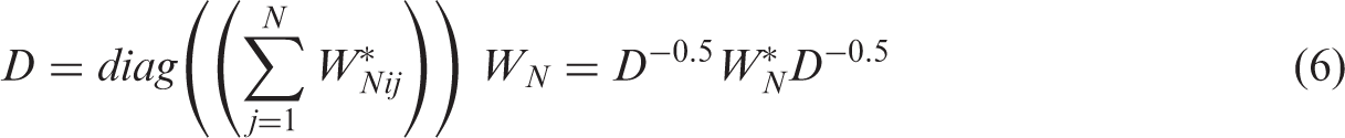
The matrix W_N is symmetrical with $W_{Nij} = W_{Nji}$ , which retains absolute rather than relative distance between MSAs as the basis of connectivity, with maximum eigenvalue equal to 1.0, which facilitates easy interpretation of $ρ_{1}$ . The continuous range for which $(I_{N} - ρ_{1} W_{N})$ is nonsingular is $1 / min (eig) < ρ_{1} < 1 / max (eig) = 1$ , and $ρ_{1}$ falling within this range is one of the conditions necessary for a stable, stationary model. Given $ρ_{1} \neq 0$ , MSA employment levels are mutually and contemporaneously interdependent, with interdependence based on geographical distance.

With regard to the dynamic element of the model, with $γ \neq 0$ there is memory in the system, so that the level of employment in an MSA is partly dependent on its level in the previous period. The mechanism operating here could be one in which the temporal lag is capturing the effect of omitted lagged values of our right hand side variables.³ It is possible to imagine these omitted lagged effects reflecting market imperfections, with the effect of change being spread over more than one period.

Spatially autoregressive disturbances

A second potential source of spatial interdependence involves the error term $ɛ_{t}$ . For simplicity we again assume an autoregressive error process defined as

\begin{matrix} ɛ_{it} = ρ_{2} \sum_{k = 1}^{N} m_{Nik} ɛ_{kt} + u_{it} \\ ɛ_{t} = (I - ρ_{2} M_{N})^{- 1} u_{t} \\ u_{it} = μ_{i} + ν_{it} \\ M_{N} = an N x N matrixofknownspatialweights (= W_{N}) \\ μ_{i} \sim iid (0, σ_{μ}^{2}) theindividual - specifictime - invarianteffect \\ ν_{it} \sim iid (0, σ_{ν}^{2}) theremaindereffectcov (μ_{i}, ν_{it}) = 0 \end{matrix}

(7)

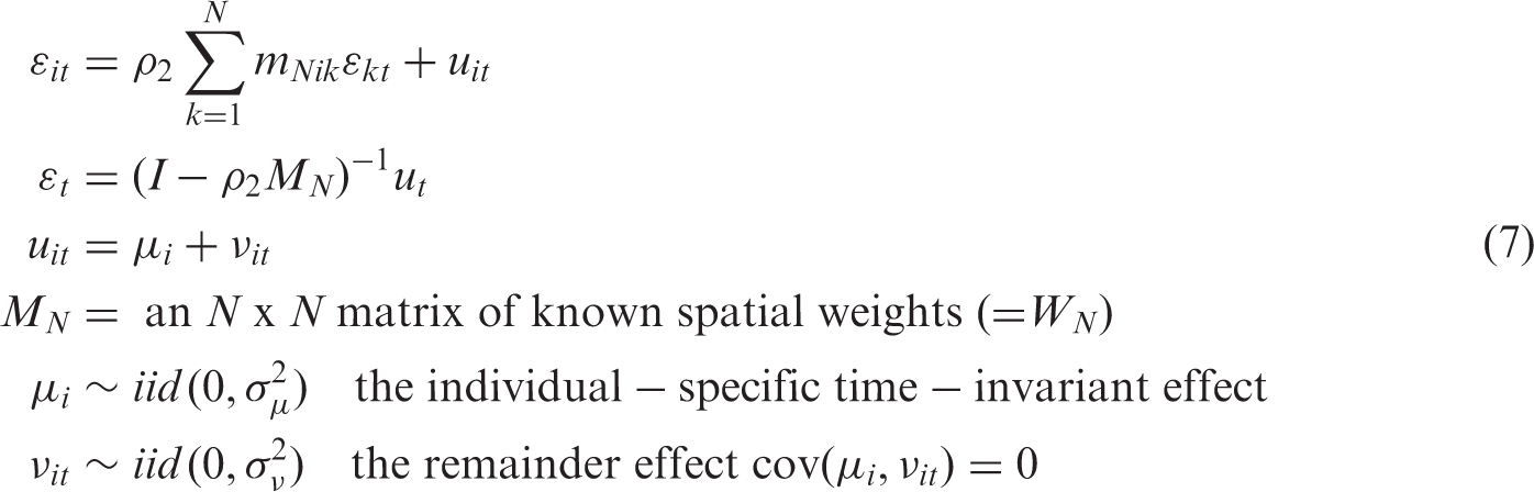
Notice here that the autoregressive error process is governed by $ρ_{2}$ which has the same stability conditions as $ρ_{1}$ , and by the weights matrix M_N, which here is identical⁴ to, and thus has the same properties as W_N. If one assumes $ρ_{2} = 0$ then there is no spillover involving the errors and $ɛ_{it} = μ_{i} + ν_{it}$ , and the error term then depends solely on the two error components, one time-invariant component $μ_{i}$ which is a set of independent draws from an $iid (0, σ_{μ}^{2})$ distribution. This term captures unobserved sources of inter-MSA heterogeneity. The component $ν_{ij}$ , which is assumed to be independent of $μ_{i}$ and distributed as $iid (0, σ_{ν}^{2})$ , picks up the remaining unobservable effects that vary across both MSA and across time.

Empirical estimation

GMM-SL-SAR-RE estimation

An estimation method for dynamic spatial panel data with random effects is given by Baltagi et al. (2014). The significant advantages of this estimator are that it allows us to incorporate a large number of regions in our analysis. In comparison, vector autoregressive (VAR) and vector error correction (VEC) modelling as applied by Papanyan (2010), Fingleton et al. (2012) and Doran and Fingleton (2014) becomes highly impractical once one extends beyond about a dozen regions and would certainly be prohibitive given 377 MSAs.

This ‘Generalized Method of Moments-Spatial Lag-Spatial Autoregressive-Random Error’ or GMM-SL-SAR-RE estimator detailed in Baltagi et al. (2014) is based on Arellano and Bond (1991), but contains additional moments to take full account of the spatial dimension of the model. It is important to mention one difference between the estimator in Baltagi et al. (2014) and the application here. In the former, the regressor(s) are assumed to be exogenous, with the exception of the endogenous lags. These then become instruments facilitating consistent estimation. However, it is unclear whether output can realistically be treated as exogenous to employment, as is evident in the exchange between Kaldor (1975) and Rowthorn (1975a, 1975b). In this paper, we assume that the regressor, $\ln x$ , is also an endogenous variable. Thus, in our estimation, we treat $\ln x$ symmetrically with regressand $\ln y$ . The standard approach with an endogenous variable as an instrument is that it should be lagged by two periods.⁵ The moments equations assume independence of the levels of the instruments and the differenced errors $Δ ν_{t} = ν_{t} - ν_{t - 1}$ , and so with an endogenous instrument such as $\ln y_{t}$ , assuming $E (Δ ν_{it}, Δ ν_{it - 2}) = 0$ , we have $cov (\ln y_{t - 2,} Δ ν_{t}) = 0$ . Therefore, in the moments conditions in the estimator, while we maintain the spatial lags of the regressand and regressors as instruments, as in Baltagi et al. (2014), we also lag the regressor $\ln x$ and its spatial lag in the same way as the endogenous regressand and its spatial lag, thus the instrument set for individual i and time t becomes

\begin{matrix} (\ln y_{i 1}, \dots, \ln y_{it - 2}, W_{N} \ln y_{i 1}, \dots, W_{N} \ln y_{it - 2}, \ln x_{i 1}, \dots, \ln x_{it - 2}, W_{N} \ln x_{i 1}, \dots, W_{N} \ln x_{it - 2}) \end{matrix}

Estimates

Applying the GMM-SL-SAR-RE estimator outlined above we obtain the estimates given in Table 1. The table shows that the coefficients are all significant and display the anticipated sign, with the values of

ρ_{1}

ρ_{2}

and γ falling with the stable bounds given in Baltagi et al. (2014).⁶

Table 1.

Parameter estimates.

Variables	Parameters	(4)
$\ln y_{t - 1}$	γ	0.4782***
		(0.0078)
$W_{N} \ln y_{t}$	$ρ_{1}$	0.2731***
		(0.0124)
$\ln x_{t}$	$β$	0.2167***
		(0.0058)
	$ρ_{2}$	0.4464
	σ²_μ	1.5638
	σ²_υ	0.2499

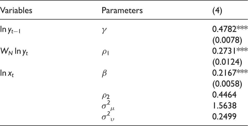
Standard errors in parentheses.

***

p < 0.01.

The estimated $ρ_{1}$ is highly significant,⁷ with a one-tailed p-value less than 0.001. The estimated $ρ_{2}$ is also significantly different from 0. For inference regarding $ρ_{2}$ , the reference distribution is obtained as a result of 100 Monte Carlo simulations in which the residuals are sampled with replacement and thus randomly allocated spatially. This has a mean equal to − 0.0445 and standard deviation equal to 0.2266, so the t-ratio is 2.17 with a two-tailed p-value equal to 0.03, indicating that estimated falls outside the sampling distribution consistent with a null hypothesis that $ρ_{2} = 0$ . Also there is a considerable amount of individual (MSA) heterogeneity as evident from the estimated variance ${\hat{σ}}_{μ}^{2}$ which is large relative to the variance of the remainder component ${\hat{σ}}_{ν}^{2}$ .

The positive association between output and employment is consistent with the theoretical model presented previously, and indicates that, controlling for endogeneity, there exists a positive causal impact of output with regards to employment. The positive spatial lag parameter ( $ρ_{1}$ ) suggests that there are simultaneous positive spatial dependencies between MSA employment levels having controlled for significant positive temporal dependence as indicated by the estimated γ.

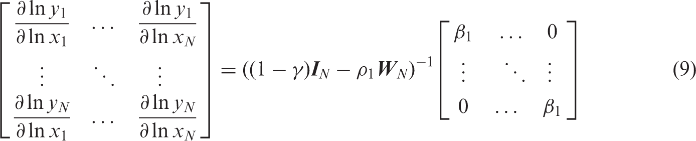
The estimates in Table 1 suggest that the constant elasticity of employment with respect to output is quite small, as indicated by $\hat{β}$ , when compared to the typical value of the Verdoorn coefficient $b \approx 0.5$ . However, the impact of output on employment as given by $\hat{β}$ is quite misleading, for it fails to take account of the spatial and temporal interactions present in the model.

It is now standard practice to acknowledge that the effect of a variable should equal the true derivative of 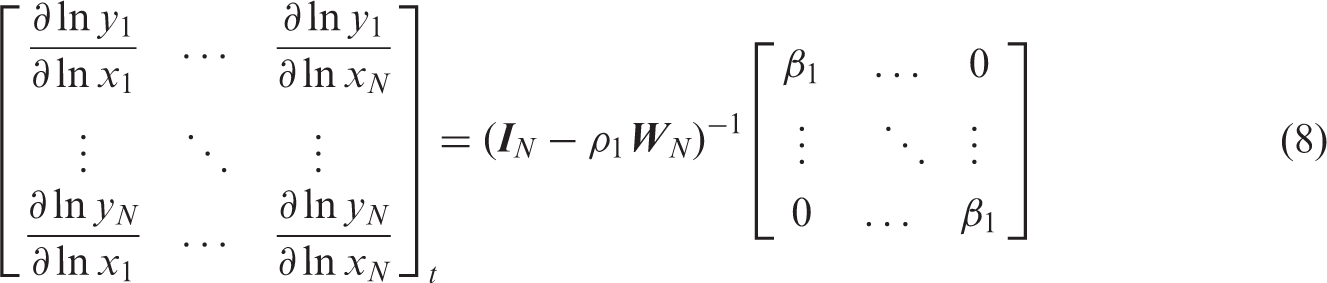$\ln y$ with respect to $\ln x$ , which in the presence of significant spatial lag and dynamic effects is not simply the estimate $\hat{β}$ [Le Sage and Pace (2009) and Elhorst (2014)]. There are both short and long run effects. The short run effects at a specific point in time t are the derivatives

\begin{matrix} [\begin{matrix} \frac{\partial \ln y_{1}}{\partial \ln x_{1}} & \dots \frac{\partial \ln y_{1}}{\partial \ln x_{N}} \\ : & : \\ \frac{\partial \ln y_{N}}{\partial \ln x_{1}} & \dots \frac{\partial \ln y_{N}}{\partial \ln x_{N}} \end{matrix}]_{t} = (I_{N} - ρ_{1} W_{N})^{- 1} [\begin{matrix} β_{1} & \dots 0 \\ : & : \\ 0 & \dots β_{1} \end{matrix}] \end{matrix}

(8)

And the long run effects are given by

\begin{matrix} [\begin{matrix} \frac{\partial \ln y_{1}}{\partial \ln x_{1}} & \dots \frac{\partial \ln y_{1}}{\partial \ln x_{N}} \\ : & : \\ \frac{\partial \ln y_{N}}{\partial \ln x_{1}} & \dots \frac{\partial \ln y_{N}}{\partial \ln x_{N}} \end{matrix}] = ((1 - γ) I_{N} - ρ_{1} W_{N})^{- 1} [\begin{matrix} β_{1} & \dots 0 \\ : & : \\ 0 & \dots β_{1} \end{matrix}] \end{matrix}

(9)

The total short run effect is the effect on

\ln y

at time t of a one unit change in

\ln x

(or equivalently a 1% change in x) in each of N regions (cities) at time t, inclusive of both direct and indirect effects. For the long run effect, the derivatives give the total effect on

\ln y

at time T (as T goes to infinity) of a one unit change in

\ln x

in each of N regions which remains through all times to T. Given the size of these matrices of derivatives, one takes the mean of the main diagonal of the matrix of partial derivatives for the direct effects, and the mean of the off-diagonal cells for the indirect effects. The sum of the two means is the total effect. Table 2 gives the results.

Table 2.

Short and long run effects (two-step estimates).

	Short run	Long run
Direct	0.2169	0.4162
Indirect	0.0797	0.4472
Total	0.2966	0.8634

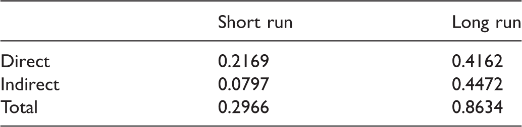
Table 2 indicates that the direct short run effect (0.2169) is slightly larger than $\hat{β} = 0.2168$ , because the direct effect also includes feedback effects due to effects passing through other MSAs and back to the original MSA.⁸ The short run indirect effect comes from the off-diagonal cells of the matrices of derivatives, and thus captures the spillover effect on employment in an MSA of a change to output in other MSAs. Adding the direct and indirect effects gives a total short run effect of 0.2966. Interestingly, the short run total effect is positive and less than one, not unlike the traditional Verdoorn coefficient $b \approx 0.5$ , suggesting that productivity depends on output in line with the increasing returns hypothesis. The total long run effect resulting from a persistent increase in output and taking into account spillovers, is an elasticity⁹ of 0.8634. This is closer to the value 1.0 consonant with constant returns to scale, but nevertheless the evidence here is that in the very long run, there remains some overall productivity gain as output increases.

Prediction and generating a counterfactual employment series

Methodology

The prediction methodology involves using the parameter estimates given in Table 1, which relate to the model set out as equation (4), in order to simulate counterfactual employment levels across the 377 MSAs. Equation (4) is repeated here, but as a recurrent equation in matrix format, as equation (10),

\ln y_{t} = G_{N}^{- 1} [γ \ln y_{t - 1} + \ln x_{t} β + B_{N}^{- 1} u_{t}]

(10)

In which $G_{N} = (I_{N} - ρ_{1} W_{N})$ and $B_{N} = (I_{N} - ρ_{2} M_{N})$ .

Following Chamberlain (1984), Sevestre and Trognon (1996) and Baltagi et al. (2014), the linear predictor is given by equation (11).

E [\ln y_{t}] = G_{N}^{- 1} (γ E [\ln y_{t - 1}] + \ln x_{t} β + B_{N}^{- 1} E [μ])

(11)

\ln {\hat{y}}_{t} = {\hat{G}}_{N}^{- 1} (\hat{γ} \ln {\hat{y}}_{t - 1} + \ln {\tilde{x}}_{t} \hat{β} + {\hat{B}}_{N}^{- 1} \hat{μ})

(12)

Equation (11) is the same as equation (10) but with expectations E[·], and this leads to equation (12) which gives the estimated expectations of (log) employment ( $\ln y_{t}$ ) based on counterfactual levels of (log) output $(\ln {\tilde{x}}_{t})$ and estimated parameters $(\hat{γ}, \hat{β}, {\hat{ρ}}_{1}, {\hat{ρ}}_{2})$ . The estimated expectations of the individual effects $\hat{μ}$ are obtained from the residuals averaged over time, as described in Appendix 2.

Generating the counterfactual series

Given equation (12), the counterfactual employment series ( $\ln {\hat{y}}_{t}$ ) depends on the counterfactual output series ( ${\tilde{x}}_{t}$ ). As we treat the 2008 economic crisis as a common shock across all MSAs (though each MSA will have reacted differently), the counterfactual output series is based on the observed national change in output over the period 2008 to 2014, an assumption that is consistent with Martin et al. (2016). The underlying assumption made here is that output in a particular MSA would contract at the national rate during a recession and expand at the national rate during a recovery were it not for differences in industrial structure. This can be represented as:

{\tilde{x}}_{it + 1} = (1 + g_{Nt + 1}) {\tilde{x}}_{it}

where

{\tilde{x}}_{it + 1}

denotes counterfactual output for period t + 1 for MSA i_,

g_{Nt + 1}

is the national growth rate of GDP from t to t + 1, and

{\tilde{x}}_{it}

is the value of output in time period t for region i. Note that

{\tilde{x}}_{it + 1}

depends on

x_{it} (t = 2007)

, the actual level of output in 2007. Subsequently, for all other

t > 2007

{\tilde{x}}_{it + 1}

depends on

{\tilde{x}}_{it}

. This gives a counterfactual level of output for each MSA assuming that the MSA output grew through the crisis at a rate identical to the national GDP growth rate. This is similar to the approach used by Martin et al. (2016), but our approach differs in that here the counterfactual is used, not to generate resilience indices per se, but to instead feed into the employment prediction equation (12).

MSA resilience to the 2007 economic crisis

Measuring elements of resilience

We focus on two elements of resilience; resistance and recovery (Martin, 2010; Martin et al., 2016; Palaskas et al., 2015). Resistance is the ability of a regional economy to resist the initial impact of the crisis; recovery is the ability to recover following the shock (Han and Goetz, 2013). Following, broadly, Han and Goetz (2013) and Martin et al. (2016), resistance and recovery are defined here by equations (13) and (14), respectively.

\begin{matrix} {Resis}_{i} = \frac{({Δ y}_{i}^{c}) - (Δ {\hat{y}}_{i}^{c})}{E_{i}^{2007}} \end{matrix}

(13)

\begin{matrix} {Recov}_{i} = \frac{({Δ y}_{i}^{r}) - (Δ {\hat{y}}_{i}^{r})}{E_{i}^{2007}} \end{matrix}

(14)

In (13), $Δ y_{i}^{c}$ is the change in employment in region i during the contraction period of the economic crisis, and in (14) $Δ y_{i}^{r}$ is employment change in region i during the post-crisis recovery period. In contrast to these actual employment changes, $Δ {\hat{y}}_{i}^{c}$ is the counterfactual employment change during contraction, and $Δ {\hat{y}}_{i}^{r}$ is the counterfactual change during recovery. Differences between actual and counterfactual are scaled by 2007 employment level $E_{i}^{2007}$ . For both $Resis$ and $Recov$ , a zero value indicates that employment changed in line with the counterfactual (based on the national change), a negative value shows relatively weak resistance/recovery and a positive value indicates stronger resistance/recovery relative to the national performance.

Testing the industrial structure hypothesis

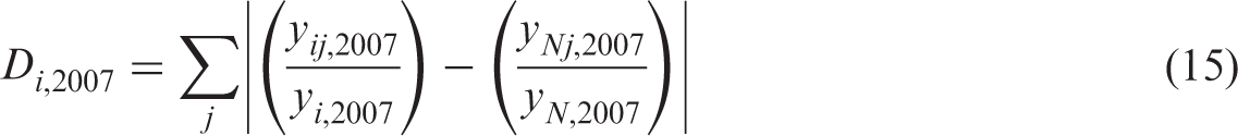
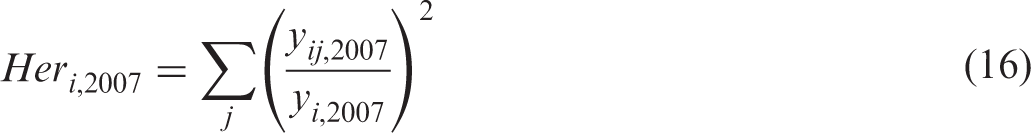
To explain inter-MSA variation in $Resis$ and $Recov$ , we calculate three industry structure variables; a Krugman dissimilarity index (15), a Herfindal index (16), and a Lilien index (17) of structural change, each of which is based on MSA employment across 13 different sectors, using data from by the American Community Survey.¹⁰

\begin{matrix} D_{i, 2007} = \sum_{j} | (\frac{y_{ij, 2007}}{y_{i, 2007}}) - (\frac{y_{Nj, 2007}}{y_{N, 2007}}) | \end{matrix}

(15)

\begin{matrix} {Her}_{i, 2007} = \sum_{j} (\frac{y_{ij, 2007}}{y_{i, 2007}})^{2} \end{matrix}

(16)

{Lilien}_{i, t} = [\sum_{j} (\frac{y_{ijt}}{y_{it}}) (Δ {logy}_{ijt} - Δ {logy}_{it})^{2}]^{1 / 2}

(17)

In equations (15), and (16), i refers to MSA i in 2007. Also $y_{ij, 2007}$ is MSA i 's industry j employment level, $y_{i, 2007}$ is total employment in MSA i, $y_{Nj, 2007}$ is total industry j employment in all MSAs, and $y_{N, 2007}$ is total employment in all MSAs.

The Krugman index $D_{i, 2007}$ , measuring industrial structure dissimilarity, ranges from zero to two, with zero indicating that MSA i’s industrial structure is identical to the national industrial structure and two indicating maximum dissimilarity (Van Egeraat et al., 2016; Goschin et al., 2009). The Herfindal index ${Her}_{i, 2007}$ measures concentration in a particular industry. The higher the index, the more specialised is an MSA (Van Egeraat et al., 2016). The ${Lilien}_{i, t}$ index measures shifts in industrial employment over a given time period (Goschin et al., 2009; Martin et al., 2016). For this, we define two time periods, the recession (2008–2009) and the recovery (2009–2014).

Given that the indices $D_{i, 2007}$ and ${Her}_{i, 2007}$ measure specialisation just prior to the onset of the crisis, the hypothesis is that an MSA’s specialization pre-crisis had an effect on its in-crisis resistance and post-crisis recovery. For the ${Lilien}_{it}$ index, measured within-crisis (2007–2009) and post-crisis (2009–2014), we explore whether contemporaneous structural change had an effect on an MSA’s resistance and recovery.

Subsequent analysis treats $Resis$ and $Recov$ , referred to collectively as $R_{i}, i = 1, \dots, n$ , as the dependent variables in regression models in which the Krugman, Herfindal and Lilien indices are the causal variables of principal interest. However, we also control for a number of covariates so as to eliminate omitted variable bias. For the Krugman, and Herfindal indices, since they are based on 2007 data, we can reasonably assume they are exogenous, and thus cause subsequent changes in R_i, in which case OLS estimation should give unbiased estimates. However, endogeneity is built in ab initio into the Lilien index since it is calculated using data from the within-crisis and post-crisis periods, respectively, so there is a possibility of resistance and recovery both being affected by, and affecting, structural change. This two-way interaction between structure and employment response is to be anticipated given the earlier discussion of adaptive resilience. To allow for potential endogeneity we apply instrumental variables.

Four instrumental variables are employed. Firstly, we use the spatial lag of ${Lilien}_{i, t}$ . Secondly, we employ Bartlett’s three group method. In this, given an endogenous variable of dimension n, its instrument is formed by dividing the variable into three categories. The n/3 smallest values are set to − 1, the n/3 largest are set to 1 and the n/3 middle values are set to zero (Johnson, 1984; Kennedy, 2008). The assumption is that while the resulting instrument will be correlated with the endogenous variable, it will be independent of the error term, as required for consistent estimation.¹¹ A third instrument is provided by the spatial lag of Bartlett’s three groups. The fourth instrument used is the synthetic instrument proposed by Le Gallo and Páez (2013). This is based on a contiguity matrix, but since MSAs are on the whole non-contiguous, we treat an MSA’s three nearest neighbours to be contiguous with the MSA. We follow Le Gallo and Páez (2013) in creating a synthetic instrument for the Lilien index by first obtaining the eigenvectors of the contiguity matrix. Then, eigenvectors are regressed on the Lilien index and the significant eigenvectors are retained and summed to create an exogenous instrument (each significant eigenvector is weighted according to the estimated regression coefficient). Utilising these instruments means that we can treat the regression coefficient relating to the Lilien index, when estimated by IV, as estimates of the change in R_i caused by a unit change in this explanatory variable.

Additional regressors (see also Han and Goetz, 2013) are introduced to avoid omitted variable bias, bias which may come about if the industrial structure indices also capture the impact of correlated variables not included explicitly in a regression specification. Consequently, we control for population density, educational attainment, sectoral composition, and the Region¹² of the US in which the MSA is located to give the model

\begin{matrix} R_{i} = β_{0} + β_{1} D_{i, 2007} + β_{2} {Her}_{i, 2007} + β_{3} {Lilien}_{it} + covariates + ɛ_{i} \end{matrix}

(18)

In (18), R_i denotes either ${Resis}_{i}$ or ${Recov}_{i}$ for MSA i, the $β s$ are the regression coefficients, $D_{i, 2007}$ is the Krugman dissimilarity index for 2007, ${Her}_{i, 2007}$ is the Herfindal concentration index for 2007, and ${Lilien}_{it}$ denotes structural change for the time periods t = 2007–2009 for ${Resis}_{i}$ and t = 2009–2014 for ${Recov}_{i}$ . The error term $ɛ_{i}$ represents additional unobserved effects, distributed as $iid (0, σ^{2})$ in which $σ^{2}$ denotes constant error variance. Equation (18) is estimated via instrumental variables (IV). In contrast to ${Lilien}_{it}$ , population density, educational attainment (the proportion of those aged over 24 with a third level degree), sectoral composition and region relate to the year 2007, and so are treated as exogenous.

Table 3 gives the IV estimates of equation (18). To save space we omit the parameter estimates of the 22 covariates (see Appendix Tables A3.1 and A3.2 for these), which are of limited interest, but we do show the overall significance of the covariates by adding them sequentially in blocks, namely demographics (population density and educational attainment), sectors (12 sector variables), and regions (8 region dummy variables), and find they are all jointly significant at the 95% level (at least) for both

{Resis}_{i}

and

{Recov}_{i}

. To support our inferences, we show instrument relevance (i.e. the extent of correlation of the IVs with

{Lilien}_{it}

) and instrument exogeneity (i.e. their lack of correlation with the errors). Following Stock et al. (2002) instrument relevance is indicated via F statistics greater than 10. Given overidentification, because we have four instruments, instrument exogeneity for the group is shown to exist using Hansen’s (1982) J statistic.¹³ In Appendix 3, we test each instrumental variable separately to identify individual relevance, to resistance (Table A3.1) and recovery (Table A3.2), showing that the most relevant instrument is Bartlett’s three group method followed by the Le Gallo and Páez (2013) synthetic instrument.

Table 3.

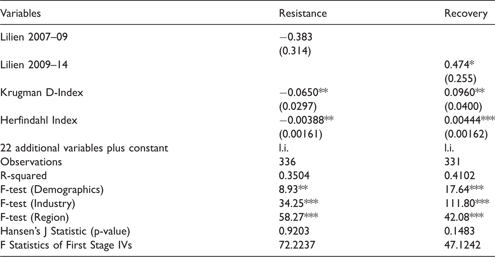
Industry structure controls and resistance and recovery.

Variables	Resistance	Recovery
Lilien 2007–09	−0.278
	(0.325)
Lilien 2009–14		0.495*
		(0.278)
Krugman D-Index	−0.0770**	0.0865**
	(0.0308)	(0.0407)
Herfindahl Index	−0.00344**	0.00508***
	(0.00165)	(0.00171)
22 additional variables plus constant	l.i.	l.i.
Observations	341	341
R-squared	0.338	0.398
F-test (Demographics)	5.99**	10.95***
F-test (Industry)	32.45***	91.44***
F-test (Region)	57.41***	31.49***
Hansen’s J Statistic (p-value)	0.7751	0.1226
F Statistics of First Stage IVs	73.5939	48.9425

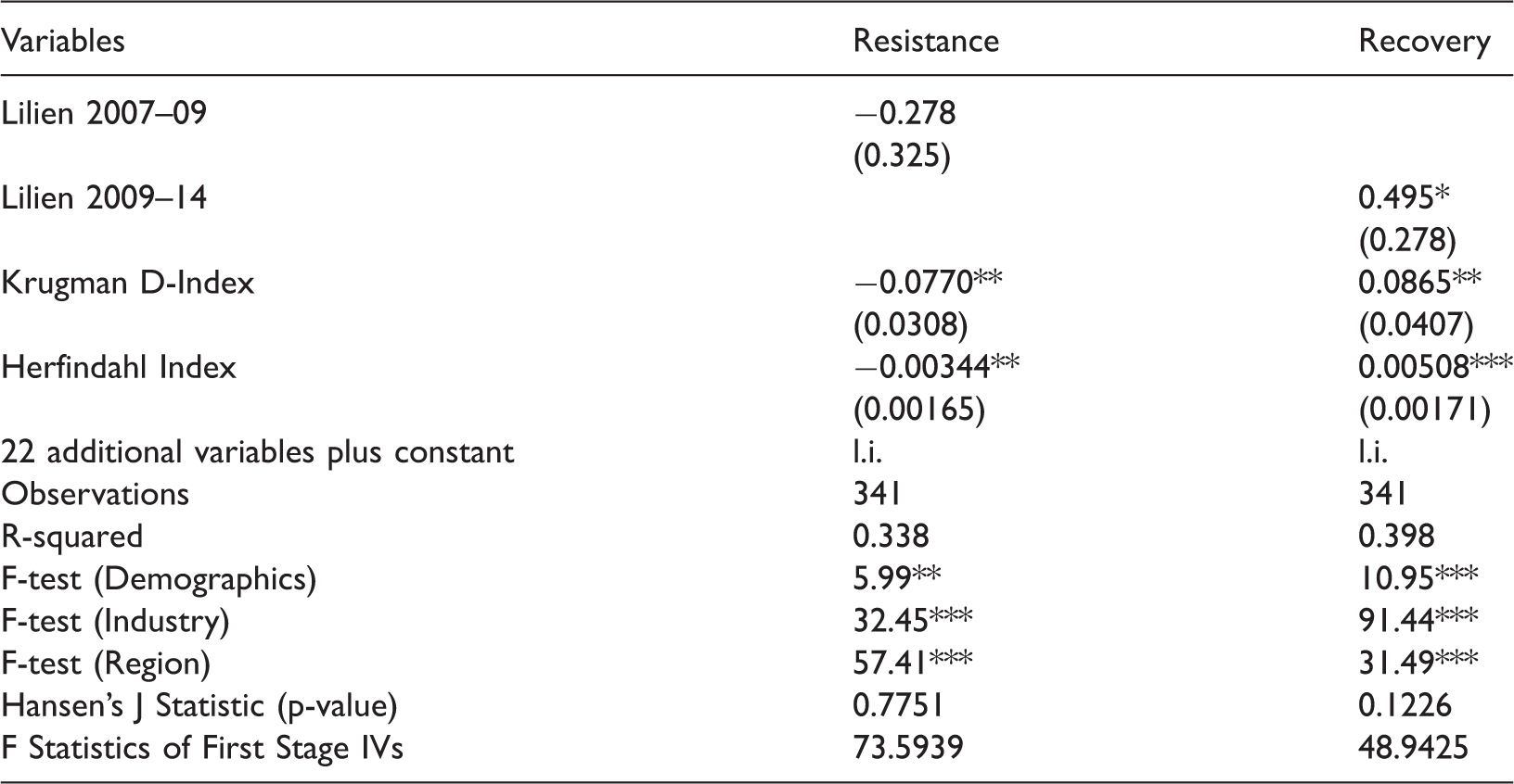
l.i. denotes of limited interest.

Note 1: Robust standard errors in parentheses.

Note 2: ***p < 0.01, **p < 0.05, *p < 0.1.

Note 3: Hansen’s (1982) J statistic chi-squared test is reported. A statistically significant test statistic always indicates that the instruments may not be valid.

Note 4: Following Stock et al. (2002) instrument relevance is indicated via F statistics greater than 10.

Table 3 indicates that the Krugman index and the Herfindahl index both have a negative effect on resistance, indicating that specialization increases susceptibility to shocks. In contrast post-crisis, specialisation appears to positively aid recoverability. Also the significant positive effect of the Lilien index suggests that shifts in industrial employment following a shock have a beneficial effect on post-shock recovery. This may reflect MSAs reorienting themselves away from impacted sectors to sectors which were not impacted by the crisis.

With regard to the control variables, our estimates indicate that MSAs with a higher percentage of the population with Bachelor degrees, or higher, are better able to resist and recover following the crisis. This points to the importance of an educated workforce, ceteris paribus, in improving an MSA’s resilience.

MSAs with a higher proportion of their workforce in construction, manufacturing, finance and insurance or other services possess lower resistance indices ceteris paribus. However, MSAs with a higher proportion of their workforce in educational services, arts, entertainment and recreational services or public administration exhibit poorer recovery post-shock. This suggests that sectoral employment differences may aid in explaining the susceptibility of MSAs, hence regions, to shock and impact their speed of recovery post-shock.

Having controlled for the above factors we still observe significant regional variations in our resistant and recovery indices. Relative to New England (the reference category) MSAs in the Middle Atlantic, West North Central, and West South Central regions have higher resistance indices ceteris paribus. When considering recovery New England and the Middle Atlantic are the regions where MSAs possess the lowest recovery indices while MSAs in the West South Central and East South Central exhibit the highest recovery indices.

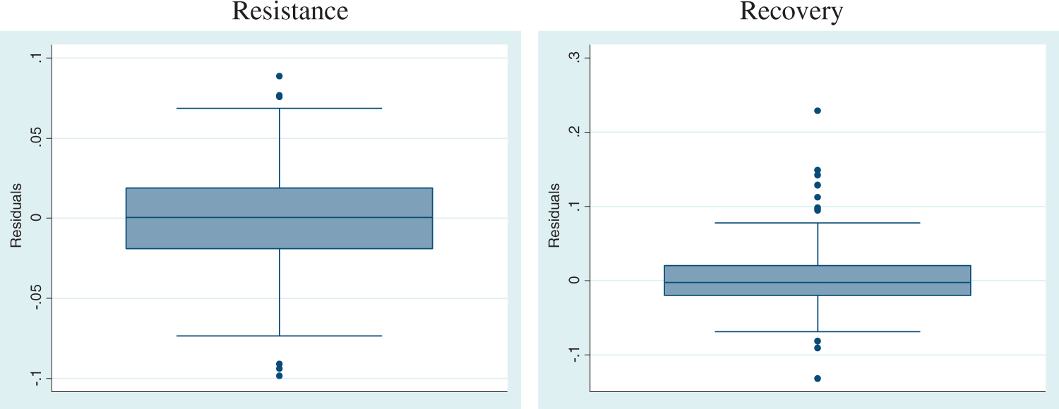
The robustness of the Table 3 inferences is predicated on error distribution assumptions. Figure 1 shows approximately normality for both $Resis$ and $Recov$ regression residuals, but Figure 2 highlights potentially influential outliers, although when excluded, as in Table 4 estimates, the results are broadly consistent with Table 3. Our key industrial structure variables remain significant and appropriately signed.

Figure 1.

Residuals of IV regression model.

Figure 2.

Box plot of residuals to identify outliers.

Table 4.

IV regression of resistance and recovery (with outliers trimmed).

Variables	Resistance	Recovery
Lilien 2007–09	−0.383
	(0.314)
Lilien 2009–14		0.474*
		(0.255)
Krugman D-Index	−0.0650**	0.0960**
	(0.0297)	(0.0400)
Herfindahl Index	−0.00388**	0.00444***
	(0.00161)	(0.00162)
22 additional variables plus constant	l.i.	l.i.
Observations	336	331
R-squared	0.3504	0.4102
F-test (Demographics)	8.93**	17.64***
F-test (Industry)	34.25***	111.80***
F-test (Region)	58.27***	42.08***
Hansen’s J Statistic (p-value)	0.9203	0.1483
F Statistics of First Stage IVs	72.2237	47.1242

l.i. denotes of limited interest.

Note 1: Robust standard errors in parentheses.

Note 2: ***p < 0.01, **p < 0.05, *p < 0.1.

Note 3: Hansen’s (1982) J statistic chi-squared test is reported. A statistically significant test statistic always indicates that the instruments may not be valid.

Note 4: Following Stock et al. (2002) instrument relevance is indicated via F statistics greater than 10.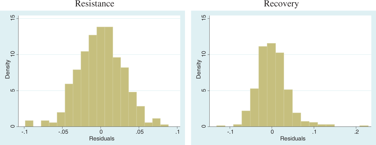

To allow for the possible presence of error dependence among the residuals, we also estimate the model with the same specification as the Table 3 model but also with an additional spatial autoregressive error term. Following Arraiz et al. (2010) and Drukker et al. (2013), via the use of instrumental variables and GMM, we obtain similar estimates to those of Tables 3 and 4, with no evidence of significant residual autocorrelation. To save space they are omitted here.

To summarize, the regression estimates show that a more specialised MSA is less resistant to shocks than a diverse MSA, and that, post-crisis, specialisation appears to positively impact an MSA’s recoverability. Also, the significant positive impact of structural change suggests that the reorientation of industrial structure following a shock aids post-shock recoverability.

Conclusions

This paper studies the effect of economic structure on the resilience of US MSAs to the 2007 economic crisis, and in doing so is one of a growing but small number of papers which analyses of resilience at a city, rather than country or regional, level [for an example of a city levels analysis see Wrigley and Dolega (2011)]. Our key findings are that MSAs which were more specialised were more adversely affected by the crisis and less able to resist it. But during the recovery phase post-crisis, we find evidence that being specialised positively affected recovery. In addition, structural change during the recovery period also had a positive effect on recovery. We also find that MSA’s sectoral composition affects resistance and recovery, but this by itself does not explain the significant regional effects. Thus, controlling for sectoral effects, the region in which an MSA is located still has an effect on resistance and recovery, although at this juncture we do not speculate about the underlying cause of the regional effects.

These interpretations are however provisional and are open to revision as longer series become available for analysis. In addition, it would be useful to look retrospectively at earlier recessions to see if more evidence could be gained regarding the determinants of resilience, taking account also of the type, strength and duration of that shock. In the past, we have seen major events such as the 1861–63 Cotton Famine, which had a major adverse impact on the towns of the Lancashire cotton district, the great stock market crash of 1929, and indeed the two World wars of 1914 and 1939, each having its own particular consequences for local, regional, national and global economies.

Footnotes

Declaration of conflicting interests

The author(s) declared no potential conflicts of interest with respect to the research, authorship, and/or publication of this article.

Funding

The author(s) received no financial support for the research, authorship, and/or publication of this article.

Notes

Appendix 1: Map of MSAs

Appendix 2 Appendix 3: Alternative IV Estimations

References

Arellano

Bond

(1991) Some tests of specification for panel data: Monte Carlo evidence and an application to employment. Review of Economic Studies 58: 277–297.

Arraiz

Drukker

Kelejian

et al. (2010) A spatial cliff-ord-type model with heteroskedastic innovations: Small and large sample results. Journal of Regional Science 50: 592–614.

Artis

Miguelez

Moreno

(2012) Agglomeration economies and regional intangible assets: An empirical investigation. Journal of Economic Geography 12: 1167–1189.

Baltagi

Fingleton

Pirotte

(2014) Estimating and forecasting with a dynamic spatial panel data model. Oxford Bulletin of Economics and Statistics 76: 112–138.

Bernat

(1996) Does manufacturing matter? A spatial econometric view of Kaldor’s laws. Journal of Regional Science 36: 463–477.

Bond

(2002) Dynamic panel data models: A guide to micro data methods and practice. Portuguese Economic Journal 1: 141–162.

Britto

McCombie

(2015) Increasing returns to scale and regions: A multilevel model for Brazil. Brazilian Keynesian Review 1: 118–134.

Bureau of Economic Analysis (2016) Regional economic accounts. Available at: www.bea.gov/regional/.

Capasso

Cefis

Frenken

(2014) On the existence of persistently outperforming firms. Industrial and Corporate Change 23: 997–1036.

10.

Chamberlain

(1984) Panel data. In: Griliches

Intriligator

(eds) The Handbook of Econometrics, Amsterdam: North-Holland, pp. 1247–1318.

11.

Christopherson

Jonathan

Tyler

(2010) Regional resilience: Theoretical and empirical perspectives. Cambridge Journal of Regions, Economy and Society 3: 3–10.

12.

Combes

P-P

(2000) Economic structure and local growth: France, 1984–1993. Journal of Urban Economics 47: 329–355.

13.

Cross

McNamara

Pokrovskii

(2010) Memory of recessions. Strathclyde – Discussion Papers in Economics 1009: 1–25.

14.

Dall’erba

Percoco

Piras

(2009) Service industry and cumulative growth in the regions of Europe. Entrepreneurship and Regional Development 21: 333–349.

15.

Dixon

Thirlwall

(1975) A model of regional growth rate differences on Kaldorian lines. Oxford Economic Papers 27: 201–214.

16.

Dixon

Thirlwall

(1978) Growth rate stability in the Kaldorian regional model. Scottish Journal of Political Economy 25: 97–99.

17.

Doran

Fingleton

(2014) Economic shocks and growth: Spatio-temporal perspectives on Europe’s economies in a time of crisis. Papers in Regional Science 93: S137–S165.

18.

Doran

Fingleton

(2015) Resilience from the micro perspective. Cambridge Journal for Regions Economy and Society 8: 205–233.

19.

Doran

Fingleton

(2016) Employment resilience in Europe and the 2008 economic crisis: Insights from micro-level data. Regional Studies 50: 644–656.

20.

Drukker

Egger

Prucha

(2013) On two-step estimation of a spatial autoregressive model with autoregressive disturbances and endogenous regressors. Econometric Reviews 32: 686–733.

21.

Elhorst

(2014) Spatial panel data models. In: Spatial Econometrics. Springer Briefs in Regional Science, Berlin, Heidelberg: Springer, pp. 37–93.

22.

Faini

(1984) Increasing returns, non-traded inputs and regional development. The Economic Journal 94: 308–323.

23.

Fingleton

(2001a) Equilibrium and economic growth: Spatial econometric models and simulations. Journal of Regional Science 41: 117–147.

24.

Fingleton

(2001b) Theoretical economic geography and spatial econometrics: Dynamic perspectives. Journal of Economic Geography 1: 201–225.

25.

Fingleton

(2003) Increasing returns: Evidence from local wage rates in Great Britain. Oxford Economic Papers 55: 716–739.

26.

Fingleton

(2014) Forecasting with dynamic spatial panel data: Practical implementation methods. Economics and Business Letters 3: 194–207.

27.

Fingleton

Garretsen

Martin

(2012) Recessionary shocks and regional employment: Evidence on the resilience of U.K. regions. Journal of Regional Science 52: 109–133.

28.

Fingleton

Garretsen

Martin

(2015) Shocking aspects of monetary union: The vulnerability of regions in Euroland. Journal of Economic Geography 15: 907–934.

29.

Fingleton

McCombie

(1998) Increasing returns and economic growth: Some evidence for manufacturing from the European Union regions. Oxford Economic Papers 50: 89–105.

30.

Fingleton

Palombi

(2013) Spatial panel data estimation, counterfactual predictions, and local economic resilience among British towns in the Victorian era. Regional Science and Urban Economics 43: 649–660.

31.

Friedman

(1964) Monetary Studies of the National Bureau. In: Spatial Econometrics. Springer Briefs in Regional Science, Berlin, Heidelberg: Springer.

32.

Friedman

(1993) The “Plucking Model” of business fluctuations revisited. Economic Inquiry 31: 171–177.

33.

Glaeser

(2005) Urban Colossus: Why is New York America’s Largest City?, Cambridge, MA: National Bureau of Economic Research.

34.

Glaeser

Ponzetto

Tobio

(2014) Cities, skills and regional change. Regional Studies 48: 7–43.

35.

Goschin

Constantin

Roman

et al. (2009) Specialisation and geographic concentration of industries in Romania. South-Eastern Europe Journal of Economics 7: 99–113.

36.

Grinfeld

Cross

Lamba

(2009) Hysteresis and economics – Taking the economic past into account. IEEE Control Systems Magazine 29: 30–43.

37.

Hans Y and Goetz SJ (2013) Predicting the economic resilience of US counties from industry input-output accounts. In: Paper presented at the Southern Regional Science Association Annual Meeting, Washington, DC, USA, 5 April 2013.

38.

Hansen

(1982) Large sample properties of generalized method of moments estimators. Econometrica: Journal of the Econometric Society 50: 1029–1054.

39.

Holm

Østergaard

(2015) Regional employment growth, shocks and regional industrial resilience: A quantitative analysis of the Danish ICT sector. Regional Studies 49: 95–112.

40.

Johnson

(1984) Econometric Methods, New York: McGraw-Hill.

41.

Kaldor

(1975) Economic growth and the Verdoorn law—A comment on Mr Rowthorn’s article. The Economic Journal 85: 891–896.

42.

Kennedy

(2008) A Guide to Econometrics, USA: Blackwell.

43.

Koyck

(1954) Distributed Lags and Investment Analysis, Amsterdam: North-Holland.

44.

Le Gallo

Páez

(2013) Using synthetic variables in instrumental variable estimation of spatial series models. Environment and Planning A 45: 2227–2242.

45.

León-Ledesma

(1999) Verdoorn’s law and increasing returns: An empirical analysis of the Spanish regions. Applied Economics Letters 6: 373–376.

46.

León-Ledesma

(2000) Economic growth and Verdoorn’s law in the Spanish regions, 1962–91. International Review of Applied Economics 14: 55–69.

47.

Le Sage

Pace

(2009) Introduction to Spatial Econometrics, Boca Raton: Taylor and Frances.

48.

McCombie

(1983) Kaldor’s laws in retrospect. Journal of Post Keynesian Economics 5: 414–429.

49.

McCombie

Roberts

(2007) Returns to scale and regional growth: The static–dynamic Verdoorn law paradox revisited. Journal of Regional Science 47: 179–208.

50.

McCombie

Spreafico

(2017) Productivity growth of the cities of Jiangsu province, China: A Kaldorian approach. International Review of Applied Economics. 1–22. DOI: 10.1080/02692171.2017.1351529.

51.

Martin

(2010) Roepke lecture in economic geography – Rethinking regional path dependence: Beyond lock-in to evolution. Economic Geography 86: 1–27.

52.

Martin

(2012) Regional economic resilience, hysteresis and recessionary shocks. Journal of Economic Geography 12: 1–32.

53.

Martin

Sunley

Gardiner

et al. (2016) How regions react to recessions: Resilience and the role of economic structure. Regional Studies 50: 561–585.

54.

Nyström

(2017) Regional resilience to displacements. Regional Studies. 1–19. DOI: 10.1080/00343404.2016.1262944.

55.

Ord

(1975) Estimation methods for models of spatial interaction. Journal of the American Statistical Association 70: 120–126.

56.

Palaskas

Psycharis

Rovolis

et al. (2015) The asymmetrical impact of the economic crisis on unemployment and welfare in Greek urban economies. Journal of Economic Geography 15: 973–1007.

57.

Papanyan

(2010) The transmission of shocks between Europe, Japan and the United States. Journal of Forecasting 29: 54–70.

58.

Phillips

Sun

Jin

(2003) Consistent HAC estimation and robust regression testing using sharp origin kernels with no truncation. Cowles Foundation for Economic Research, New Haven, Connecticut: Yale University.

59.

Piras

Postiglione

Aroca

(2012) Specialization, R&D and productivity growth: Evidence from EU regions. The Annals of Regional Science 49: 35–51.

60.

Pons-Novell

Viladecans-Marsal

(1999) Kaldor’s laws and spatial dependence: Evidence for the European regions. Regional Studies 33: 443–451.

61.

Quigley

(1998) Urban diversity and economic growth. The Journal of Economic Perspectives 12: 127–138.

62.

Romer

(2001) Advanced Macroeconomics, New York: McGraw Hill.

63.

Rowthorn

(1975a) A reply to Lord Kaldor’s comment. The Economic Journal 85: 897–901.

64.

Rowthorn

(1975b) What remains of Kaldor’s law? The Economic Journal 85: 10–19.

65.

Sevestre

Trognon

(1996) Dynamic linear models. In: Matyas

Sevestre

(eds) The Econometrics of Panel Data: A Handbook of Theory with Applications, Dordrecht: Kluwer Academic Publishers, pp. 121–144.

66.

Simmie

Martin

(2010) The economic resilience of regions: Towards an evolutionary approach. Cambridge Journal of Regions, Economy and Society 3: 27–43.

67.

Stock

Wright

Yogo

(2002) A survey of weak instruments and weak identification in generalized method of moments. Journal of Business & Economic Statistics 20: 518–529.

68.

Thirlwall

McCombie

(1994) Economic Growth and the Balance-of-Payments Constraint, Grã-Bretanha (primeira publicação): Macmillan Press Ltd.

69.

United States Census Bureau (2012) Metropolitan and micropolitan. Available at: www.census.gov/population/metro/.

70.

Van Egeraat C, Morgenroth E, Kroes R, et al. (2016) A measure for identifying substantial geographic concentrations. Papers in Regional Science. DOI: 10.1111/pirs.12241.

71.

Verdoorn

(1949) Fattori che Regolano lo Sviluppo della Produttivitá del Lavoro. L’Industria 1: 3–10.

72.

Watson

(2003) A Practical Introduction to Econometric Methods: Classical and Modern, West Indies: University of the West Indies Press.

73.

Wrigley

Dolega

(2011) Resilience, fragility, and adaptation: New evidence on the performance of UK high streets during global economic crisis and its policy implications. Environment and Planning A 43: 2337–2363.