Housing affordability: Is new local supply the key?

Abstract

This paper seeks to predict the impact of future housing supply on the affordability of residential space in the United Kingdom, using quantitative model-based simulation methods. Our spatially disaggregated analysis focuses on the greater South East region, approximately within 1.5 hours commuting time from Central London. A dynamic spatial panel model is applied to account for observed temporal variations in property prices and housing affordability across districts. The dynamic structure of this model allows us to assess the scale and extent of knock-on effects of local supply shocks in one district on other districts in the region. These complex spatial effects have been largely ignored in local or regional housing market forecasting models to date. Applying this model, we are able to demonstrate that local house prices and affordability are not only determined by the underlying supply and demand conditions in the market in question, but also depend crucially on conditions in neighbouring housing markets whose properties can be considered close substitutes within a larger regional housing market. We also show that increasing housing supply in the most critical areas has little impact on (both local and regional) affordability, even if wages do not change in response to an increase in employment.

Keywords

Local supply shocks dynamic spatial panel analysis housing affordability house price forecasts

Introduction

Although there is no consensus on the causes of unaffordable housing or even whether its existence proves that markets are imperfect, the detrimental social and financial impact to the large number of individuals and households negatively affected by it are virtually undisputed. In the USA, government and business leaders struggle to agree on strategies for combating the issue (Glaeser and Gyourko, 2003), while in the UK, the principal government policy is to increase the supply of housing in key areas to improve affordability. This simple approach is based on the fundamental assumption that increasing supply will reduce prices. However, Crook et al. (2010) show that providing new homes in the most critical areas seems to have little effect on affordability. Although Glaeser et al. (2006) argue that this may be due to higher wages offered to new residents, we show that even with exogenous wages new supply has a very small effect on local affordability.

This paper explores how dynamic spatial panel data modelling and simulation methodology can be used to assess the extent to which new housing stock makes housing more affordable, following the work of Meen et al. (2005) and Fingleton (2008) in particular. The approach is somewhat different from the complex modelling carried out by Meen et al. (2005), and more in line with the simpler approach of Fingleton (2008), which allows an element of theoretical coherence throughout. Although there are alternatives that have been suggested in the literature, we measure affordability simply as the ratio of house prices to mean annual wage levels. Other measures include the median house price to median income ratio, which can be adapted to focus on access to housing by using the lowest quartile house price to lowest quartile income ratio, or the proportion of households that can only afford acceptable accommodation with assistance.¹ However, the price to wage ratio is easy to implement and is the measure that has captured the attention of politicians.² It is also commonly used to examine the wider impact of housing affordability. For example, there is an important environmental aspect to the issue of affordability since, if housing is largely unaffordable where people work, high volumes of commuting are likely to occur (Sultana, 2002).

The focus of the analysis is the South East of England, where lack of affordability is probably at its most acute in the UK. This includes Central London, which is the major centre of employment and also where house prices are the highest in the country. As in many great cities, daily ebb and flow of commuters from more affordable locations to employment centres has a costly financial impact on individual households and on local and global environments (Tse and Chan, 2003). There are also additional macroeconomic and regional economic issues because relatively low affordability in a core region with a high level of labour demand will inhibit the inward mobility of labour. Naturally, this leads to feedback effects between house prices and local economies and other endogenous processes that simultaneously influence them. Our estimation approach adjusts for using a first-difference model and instrumenting supply and demand indicators with their lagged values. We test the validity of our estimates and the contribution of individual factors to price changes using one-step-ahead predictions. The results show that spatial and temporal lags are critical to increasing forecasting accuracy.

One of the suggested solutions to housing affordability issues is increasing local supply in the most problematic areas (Meen et al., 2005). Fundamental economic logic dictates that increasing supply should reduce prices. However, in the context of complex interaction effects between commutable areas caused by commuting flow patterns, it is difficult to easily quantify the impact of new supply on house prices and their affordability. The overall impact depends not only on income but also on income elasticity of demand in the area where supply increases. In fact, many studies show that increasing housing supply may eventually lead to rising demand (Ball et al., 2010; Fingleton, 2008; Szumilo et al., 2017). The objective of this study is to examine whether new local supplies of dwellings can improve housing affordability both within the growing location and in the region. To this end, we develop a model of house prices that allows affordability to react differently to changes in wages and employment. By assuming that wages are exogenous but allowing employment to depend on housing supply, we show how new housing may lead to lower affordability. Since allowing workers to travel between districts leads to demand interactions between locations, we also allow for a spatial effect in prices. Our estimation approach is based on a reduced form equation which allows us to simulate the impact of new supply on affordability ratios. The advantage of this approach is that, unlike interpreting model coefficients, it allows one to quantify not only the magnitude but also spatial distribution of the impact of new supply on affordability. Empirical predictions are made for a hypothetical increase in housing stock of 5% and 15% in each of London’s 32 boroughs. We also examine Cheshire’s (2014) suggestion that building 1.6 million houses on London’s greenbelt would make housing more affordable. We analyse two different versions of our empirical predictions, assuming that increased supply either interacts with demand or has no effect on it. Overall, supply is found to have a much smaller effect on affordability than expected. Furthermore, it appears that even if supply is increased in all areas by an equal margin, the impact on prices would not be distributed evenly across space.

The next section reviews different definitions of affordability and the economic significance of the concept. We then summarise our data. The following section presents the rationale behind the research question and the economic logic that leads to it, after which we discuss our estimation methods. The final two sections present our empirical predictions and conclusions.

Defining housing affordability

Despite the fact that its analytical definition has evolved over the last two decades, affordability remains an elusive concept (Stone, 2006). In fact, designing an affordability policy is hampered by the lack of a commonly accepted definition. Reducing house prices appears to be a recurring recommendation of many researchers (Bramley, 1994; Hilber and Vermeulen 2016), but measuring the impact of this approach requires a sound definition of affordability as well as an understanding of the market mechanisms underlying house price formation.

The concept of affordability

The definition of affordability adopted in this article is simply the ratio of house prices to wages. However, several other metrics have been proposed in the literature. Stone (2006) alludes to four types of affordability: relative, subjective, budget standards-based and residual income-based. Although they are conceptually very similar, small differences make each class appropriate for different applications.

Relative affordability refers to changes in the relationship between summary measures of house prices or costs and household incomes. At its core, this is a form of the price–wage ratio approach that allows one to focus more on affordability to potential house buyers. This approach is clearly useful to lenders who focus on transactions, but offers little information about affordability from the perspective of house owners.

Subjective affordability is based on market efficiency and the assumption that all households make rational decisions. In this context, all houses are occupied by people who have decided that they can afford it. Consequently, it makes little sense to define housing affordability, as in efficient markets all households would sort themselves only into dwellings they can afford. However, as Stone (2006) points out, there is a considerable difference in the discretion of income allocation to housing costs versus other costs between high- and low-income households. This means that the subjective experience of affordability of housing between the two would differ considerably.

The family budget standards approach to housing affordability is based on an analysis of different measures of how much of it should be dedicated to housing costs. If a monetary amount necessary to achieve a certain standard of living is determined (e.g. the poverty threshold; Bernstein et al. 2000), then the minimum income required to support a household in a certain area can be established. In the context of housing, this is very similar to the price–wage ratio approach as the two must stay in a certain relation to each other to ensure that households are not pushed into poverty. However, while the approach works well for perishable homogeneous goods, it is difficult to establish universal poverty thresholds for housing. Even if physical standards could be established, the corresponding monetary amount would be very difficult to find (see Stone, 2006 for more details).

The residual income approach adopts a slightly different perspective on disposable income and recognises that housing costs are one of the largest and least flexible items in household budgets. This means that income adequacy should not be defined by its overall level but by the amount left after paying for adequate housing. This controls for different sizes and types of households which, with the same level of disposable income, may require different amounts for non-shelter goods. Although this may be the most comprehensive indicator of affordability, its practical application requires defining a standard level of income that would be considered as adequate for non-housing goods. As this benchmark is likely to change over space and time, the residual approach cannot be universally applied.

The idea that housing cost should not exceed a certain proportion of household income is common to all of these metrics. This allows the ratio approach to be a useful metric as the proportion of the budget taken up by housing costs can be changed by variations in either (or both) of the two variables. While the residual approach may be the most comprehensive, the focus of this study is on measuring changes of affordability over time and comparing them across different locations, rather than against a general benchmark. We do not define nor rely on defining affordable housing, but use the ratio as its measure to quantify its relation to other economic variables and responses to policy.

Affordability and policy

In the UK, the government policy is to increase the supply of housing in order to improve affordability in the greater South East. This appears to be a natural response to rising house prices and reports of housing shortages (Barker, 2004). With White and Allmendinger (2003) as well as Whitehead (2007) arguing that housing shortages are a result of strict planning policies, it appears that the government has a key role to play in resolving the housing crisis. As Gurran and Whitehead (2011) argue, a new supply of affordable units is a function of planning regulations, development controls and fees. Since all of those factors can be affected by policy, it appears that the recipe for increasing housing affordability may be quite simple. However, despite policy design that supports provision of affordable housing and generous incentives for such developments (Morrison and Monk, 2006), the problem remains unresolved. In fact, Crook et al. (2010) show that existing policies produce a supply of dwellings that is lower than expected but also that building new homes in the most critical areas has little effect on affordability.

More recent studies indicate that simply increasing supply may not be sufficient to reduce prices. Fingleton (2008) notes that both supply and demand factors need to be considered when trying to design policies that affect house prices. If the increase in the supply of housing is accompanied by expansion of employment, there might be a feedback effect on demand for residential properties. This resonates with the argument presented by other researchers (Glaeser et al., 2006; Szumilo et al., 2017), who note a reciprocal relationship between city size, productivity and income. Gurran and Whitehead (2011) also argue that supply-focused policies may be misguided and that demand also needs to be addressed. The key concept is that under certain conditions expansion of supply can increase demand and lead to higher prices (Nelson et al., 2002).

Measuring housing affordability

The previous section showed that an analysis using a simplistic definition of affordability is likely to yield misleading results due to the large variations in building stock, regional wealth and endowment with local amenities and production factors that are reflected in house prices. Therefore, a conceptual framework is required that takes these factors into account. An obvious starting point is the quintessential urban economics models of urban house price determinants, the Alonso–Muth–Mills model, which assumes that locations closer to an urban and/or major employment centre are more attractive due to greater accessibility and shorter commutes, and will hence command higher land and house prices. Households maximise their utility by trading off the accessibility and other amenities of a given location with the cost of housing and transportation. The cost of housing is assumed to fall linearly as transport costs increase with distance to the centre, which means that the sum of these two key costs is assumed to remain constant across space. However, households, particularly those with higher incomes, are able to gain higher utility by consuming more floor space on larger parcels of land in more peripheral locations, which may more than offset the additional cost of longer commutes and travel times. While the Alonso–Muth–Mills model explains the general price distribution within a city, it fails to explain price differentials across cities. To this end, Rosen (1979) and Roback (1982) incorporate the role of wages and rents in household location choices. In the Rosen–Roback model, prices reflect wage levels and/or the aggregate value of amenities across cities. Roback’s empirical analysis infers the implicit willingness to pay for location amenities by comparing wages net of housing costs across cities, and finds that workers accept lower real wages in areas with a high level of amenities. This finding was also confirmed for the UK housing market by Gibbons et al. (2011, 2014).

Fundamental determinants of house prices

Glaeser et al. (2006) demonstrate that new supply plays a crucial role in determining whether productivity increases will lead to urban expansion or just to more expensive homes and higher wages. The former is shown to occur in places with low regulation and low density, while the latter is associated with cities marked by high density and strict planning regulations. Where housing supply is extremely inelastic, population size remains constant and wages increase to offset the accompanying rise in house prices following an increase in demand. However, these constraints can be partially circumvented by longer commutes from areas with more elastic supply and by pricing out and replacing existing low-skilled residents by highly skilled, more productive incoming workers. This is not undisputed, however, as Ortalo-Magne and Rady (2006) demonstrate that established long-term homeowners typically remain in a neighbourhood even if they could afford a larger property elsewhere following sharp house price increases in their neighbourhood. Competition for available properties is then restricted to highly skilled affluent newcomers. By contrast, pricing-out may occur where households are mainly renters and not protected by strict regulations on rent increases.

Differences between short- and long-run house price determinants are also expounded in the literature. For example, MacDonald and Taylor (1993) explore the long-run relationships between house prices in the UK and then work out potential ripple effects and short-term dynamics. More recently, Gallin (2006) investigated the long-run relationship between house prices and income and did not find a significant association. Generally, long-term house price determinants include demographic trends, household size, household income, taxation of homeownership as well as transportation cost and technology, while short-term factors include unemployment, interest rates, access to mortgage debt and the financial performance of competing asset classes (Malpezzi, 1999; Meen, 2002; Weiner and Fuerst, 2017).

Inelastic supply of housing has been shown theoretically and empirically to inflate house prices in the presence of rising demand. This may lead to house prices growing faster than wages, thereby eroding affordability. While this outcome is not desirable from a policy and household purchasing power point of view, it could be argued that if increased demand for housing is correlated with growing demand for labour, the local economy still benefits from lower unemployment rates and higher wages. While the benefit of higher earnings would be offset partially or completely by the inflation of house prices, higher employment is expected to persist. This would also be true at a national level, assuming that the size of the labour force is constant. In that case, if a growing economy wanted to sustain its development by increasing its total employment, it would have no choice but to hire and train previously unemployed workers (Aslund and Rooth, 2007). However, at a regional level, the size of the labour force could evolve as the transport infrastructure changes. Given satisfactory transportation links, the labour force would not be constant despite the fact that local population in the centre of employment may remain unchanged and limited by an inelastic supply of housing (Haynes, 1997). This shows that when analysing a particular housing market, its interaction with commutable areas also needs to be examined. Hence, the current study can be seen as an extension of the work presented by Glaeser et al. (2006), who assume that there is no cross-area commuting and model house prices based on within-area supply and demand. However, the present analysis relaxes the assumption that demand is only driven by local employment by also taking moving and commuting across areas into account.

Modelling the interaction between housing and labour markets

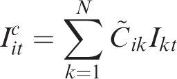
Workers who purchase or rent homes in expensive locations would be those with the highest utility derived from doing so. For example, senior workers whose opportunity cost of commuting is high could be more likely to live close to their workplace (Bissell, 2014; Eliasson et al., 2003). In a competitive bidding process, prices would increase and houses would be more likely to be occupied by those who derive higher utility from living close to the centre. However, it is also important to consider that those who have the ability to pay more are likely to outbid those whose maximum price is constrained not by their utility but by their wage (Sa, 2015). Consequently, house prices in any district are likely to be determined by wages offered to those who work there and the number of workers competing for housing in the location. While not everyone may prefer to live close to their workplace, those with higher wages can afford to pay higher prices in exchange for a less onerous commute. If income (I) in area i at time t is defined by the Hadamard (cell-by-cell) product of the N × 1 vector of mean employee mean wage rate ${\bar{w}}_{t}$ and number of employees working in each district $E_{t}$ , hence $I_{i t} = {\bar{w}}_{i t} \circ E_{i t}$ , then its growth can be driven by changes in either of those values. However, they are likely to have different effects on the affordability ratio defined as $\frac{p_{i t}}{{\bar{w}}_{i t}}$ (where p is price). If residential demand ( $q_{i t}$ ) is driven primarily by changes in income, $q_{i t} = f (p_{i t}, I_{i t})$ , then as income grows, house prices increase accordingly (Goodman, 1988). However, the impact of this process on the affordability ratio depends on whether the higher income is driven by employment or wages. While both can impact prices through demand, only wages can induce a corresponding change in the affordability ratio. In this light, an expansion of housing supply can be seen as an increase in the number of local workers. This will increase income and house prices unless it is accompanied by a reduction in average wage levels. Glaeser et al. (2006) present this process by introducing a wage model that assumes that agglomeration benefits have a positive effect, while a negative reaction is caused by the increasing labour supply. We adopt a simpler approach in which we do not allow wages to be a function of the local labour force, but assume that they are set exogenously for each district. This focuses our study on the housing demand created by the increase in employment levels and ignores the impact of additional density on wages. Omitting the density effect simplifies our analysis and assumes that the impact of new housing supply on demand is lower by ignoring one of the channels of its transmission. According to Fingleton (2008), doubling employment density in UK districts increases wages by 2.8%. This effect is unlikely to have a significant impact on our analysis as the highest changes in employment density in our simulation will not exceed 50%, so changes in wages will be very small. Moreover, if this assumption has any effect on our estimates it would be a small downward bias in the impact of new supply on prices. In our set-up, new housing supply increases income by allowing more workers (rather than higher wages). In turn, this is likely to lead to a higher housing demand. Ultimately, the impact of new supply on affordability will depend on income elasticity of demand and supply elasticities of both income and price.

While a similar process has been shown by Glaeser et al. (2006), their work has explicitly ignored any interactions between locations. If the demand for housing from residents of any district is allowed to depend on income earned by residents commuting to jobs located within commuting distance of that district, it becomes necessary to consider how this interaction may affect the impact of supply increases on prices. In other words, the jobs that determine local income are not local but distributed across commutable areas (Mulalic et al., 2014). This means that the impact of increasing local supply in district i will be affected by demand generated by commutable jobs, which we denote by $I_{i t}^{c}$ , which is income within commuting distance. We also include a spatial price-dependence element $(W_{N} p)$ and two district-invariant variables in the demand function, $B_{t}$ and $F_{t}$ , which becomes $q_{i t} = f (p_{i t}, I_{i t}^{c}, W_{N} p_{i t}, B_{t}, F_{t})$ . This reflects the fact that demand for property $q_{i t}$ depends not only on local prices and income within commuting distance, but on prices in ‘nearby’ districts, where ‘nearby’ means within commuting range, and on the Bank of England interest rate $B_{t}$ and the FTSE ALL SHARES index of share prices, $F_{t}$ .³ In order to calculate the mean bank interest rate for each year, we take the mean of the rates applying in each month of the year. The bank interest rate is proposed to capture the effect on demand of (closely related) mortgage interest rates. It also reflects returns on investments held as bank deposits, as an alternative to property investment. The mean FTSE ALL SHARES index is similarly meant to capture competing investment opportunities. Its annual value is calculated as the average level of monthly closing values of the index, as reported by Bloomberg.

We assume that prices will be correlated contemporaneously across space. That means that prices will tend to be related in districts that are close together in space as well as in time. For example, two identical properties on either side of a street would undoubtedly see a convergence in price because of comparison effects. We can think of this as a displaced demand effect, whereby an initially more expensive property would displace demand to a closely comparable property, thus lowering the price of one and raising the price of the other until an equilibrium is reached. We envisage a similar process operating at the district level, where, having controlled for other factors affecting prices, including inter-district heterogeneity, there will be a tendency for prices to converge in locations where price comparisons are being made. Critically, however, we assume that those comparisons will be made based on commuting possibilities between zones as workers from each district affect the demand in its commutable areas.

Introducing this regional price interaction between commutable areas needs to be put in the context of the imperfections of both real estate and labour markets that determine it. Both markets are characterised by long search times, sticky prices and high transaction costs (Lambson et al., 2004). This results in changes occurring slowly and current prices being highly dependent on their historical values. One way to visualise this is as an imperfection in the market, so that the full effect of a change in price is not felt immediately. One might imagine that the full effect of rising prices will be moderated by institutional rigidities in the housing market, so that consumers already locked into the purchasing process will maintain their demand despite a price shock because of the costs of withdrawal due to commitments already entered into. Similarly, a delayed response to rising prices may be the outcome of imperfect knowledge of substitutes – for example, there will be a cost of acquiring knowledge of, and access to, the rental market. We assume that the effect of a price adjustment is distributed over two years rather than being instantaneous. Including lagged prices in both supply and demand is consistent with the work of Meen (2005) and Holly et al. (2011) for the UK, and with the approach of Iacoviello (2005) for the USA. While this spatial dependency necessitates including a temporal lag factor ( $P_{i t - 1}$ ) into the demand equation, it presents an interesting problem in the light of the spatial correlation in house prices. If district-specific demand effects are distributed over two time periods, then their spatial effects should not be assumed to occur instantly but to follow the same temporal process. It appears that a temporal lag of the spatial lag ( $W P_{i t - 1}$ ) also needs to be included in the model to control for this process. Baltagi et al. (2018) show that this term with a negative coefficient, as in Table 2, is a concomitant feature of an equilibrium process.

Table 1.

Summary statistics and differences between districts over time.

	House prices		Affordability		Wages		Population		Density
	Average	SD	Average	SD	Average	SD	Average	SD	Average	SD
2008
London borough	296,881	7733	9.12	1.72	593.1	80.4	243,906	51,485	66.86	33.76
Metropolitan district	130,330	18,923	5.49	0.51	438.4	30.2	312,408	174,472	20.06	9.75
Non-metro	193,004	52,828	7.30	1.48	486.9	68.5	104,320	28,994	7.16	8.62
Unitary authority	164,932	48,724	6.46	1.34	467.8	66.9	187,262	68,241	18.47	15.52
2012
London borough	323,533	133,285	9.40	2.71	623.3	70.6	259,406	56,594	71.03	35.83
Metropolitan district	123,090	20,862	4.88	0.53	465.7	35.3	320,878	182,937	20.59	10.25
Non-metro	190,390	58,938	6.77	1.50	514.8	71.1	106,957	30,230	7.38	8.97
Unitary authority	160,985	51,646	5.99	1.35	491.1	66.8	193,394	71,712	19.18	16.30

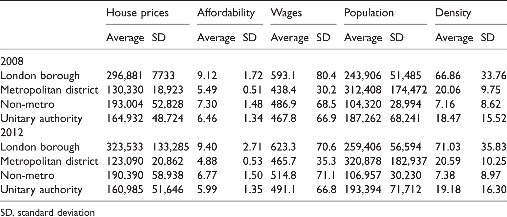
SD, standard deviation

Table 2.

GMM-SL-SAR-RE estimates of the dynamic spatial panel model.

Parameter	Estimate	Standard error	t ratio
$γ$	0.9518	0.001283	742.1
$ρ_{1}$	0.583	0.004454	130.9
$β_{1}$	270.3	6.663	40.57
$β_{2}$	–0.9701	0.02689	–36.08
$β_{3}$	–1.687	0.02743	–61.5
$β_{4}$	–4.016	0.06409	–62.67
$θ$	–0.585	0.004215	–138.8
$ρ_{2}$	0.4555
$σ_{μ}^{2}$	3.6806
$σ_{ν}^{2}$	2.1518

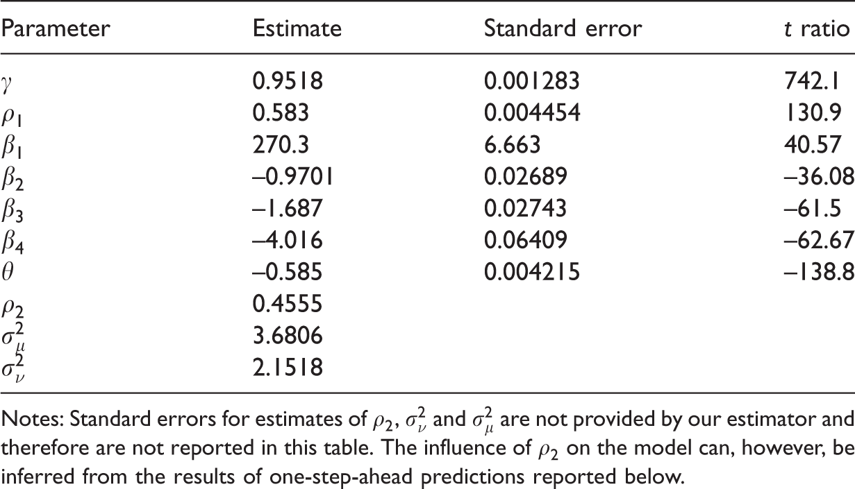
Notes: Standard errors for estimates of $ρ_{2}$ , $σ_{ν}^{2}$ and $σ_{μ}^{2}$ are not provided by our estimator and therefore are not reported in this table. The influence of $ρ_{2}$ on the model can, however, be inferred from the results of one-step-ahead predictions reported below.

Table 3.

RMSEs for one-step-ahead predictions given by prediction equation (9) and sub-models.

Full model	$ρ_{1} = 0$	$γ = 0$	$θ = 0$	$β_{1} = 0$	$β_{2} = 0$	$ρ_{2} = 0$	$β_{3} = 0$	$β_{4} = 0$
17.4213	168.8065	641.2378	445.7474	58.7971	201.8032	93.0538	203.7190	230.2032

Table 4.

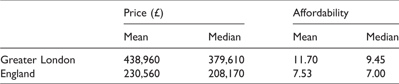
Actual prices and affordability in 2012.

	Price (£)		Affordability
	Mean	Median	Mean	Median
Greater London	438,960	379,610	11.70	9.45
England	230,560	208,170	7.53	7.00

There are also potentially additional unmeasured effects, such as demand coming from non-wage earners, local taxes and amenities and the likely returns from investing in a neighbourhood.⁴ These unmeasured effects, accounting for time-constant across-district heterogeneity together with additional transient effects, are represented in our model by random disturbances, $ω_{i t}$ . Finally, for each of the districts included in our analysis, the proposed demand function can be formalised as:

q_{i t} = f (p_{i t}, p_{i t - 1}, I_{i t}^{c}, W_{N} p_{i t}, B_{t}, F_{t}, W_{N} p_{i t - 1}, ω_{i t})

where

q_{i t}

is the demand for housing in district i (i = 1,…,N) at time t;

I_{i t}^{c}

is income within commuting distance;

p_{i t}

and

p_{i t - 1}

are prices and prices lagged by one year;

W_{N} p_{i t}

is the spatial lag of prices;

B_{t}

and

F_{t}

are the bank rate and FTSE share index respectively;

W_{N} p_{i t - 1}

is the spatial lag of the temporal lag of prices; and

ω_{i t}

represents other unmeasurable factors. To obtain

I_{i t}^{c}

we commence with income by district,

I_{i t}

, thus:

I_{i t} = {\bar{w}}_{i t} \circ E_{i t}

which gives

I_{i t}^{c} = \sum_{k = 1}^{N} {\tilde{C}}_{i k} I_{k t}

where

_{\tilde{C}}

is an N × N matrix in which row i (i = 1,…,N) contains the proportions of commuters travelling from district i to work in each of the N districts.⁵

We assume that price comparisons will involve districts with similar locations with respect to the location of employment, and we measure this similarity using an N × N proximity matrix, $W_{N}$ . The effect of proximate prices is captured in the model by the vector $W_{N} p_{t}$ , which is the matrix product of $W_{N}$ and the price vector $p_{t}$ , thus:

W_{N} p_{i t} = \sum_{k = 1}^{N} w_{i k} p_{k t}

Since large inter-district commuting flows are a good indicator of close proximity, the matrix $W_{N}$ is taken to be the same as the weighting matrix used to give $I_{t}^{c}$ , except that the leading diagonal cells are set to zero prior to standardisation.⁶ Accordingly, cell i of vector $W_{N} p_{t}$ is a weighted average of districts in the vicinity of i, with weights determined by proximity as given by inter-district commuting frequencies. Moreover, because of market imperfections there is also an effect of proximate prices in the previous period, hence we include $W_{N} p_{t - 1}$ in the specification.

We assume a linear demand function, with negative coefficients on price, except on the spatial lags of price where the displaced demand would tend to a negative relationship. However, in our reduced form this is not identified so we do not explicitly test this hypothesis. We also anticipate that a higher bank rate with correspondingly higher mortgage rates and higher returns from savings will be associated with lower demand, and similarly a higher FTSE index indicates lower demand for housing, with investment attracted to higher returns in stocks and shares than property:

q_{i t} = a_{1} I_{i t}^{c} - a_{2} p_{i t} - a_{3} p_{i t - 1} + a_{4} W_{N} p_{i t} - a_{5} B_{t} - a_{6} F_{t} + a_{7} W_{N} p_{i t - 1} + ω_{i t}

(1)

On the supply side, the variables are the same, except that we substitute the stock of dwellings ( $S_{i t}$ ) for income within commuting distance, and there are different assumptions about the signs on the coefficients. This is apparent from equation (2):

\begin{array}{l} q_{i t} = f (p_{i t}, p_{i t - 1}, S_{i t}, W_{N} p_{i t}, B_{t}, F_{t}, W_{N} p_{i t - 1}, ς_{i t}) \\ q_{i t} = b_{1} p_{i t} + b_{2} p_{i t - 1} + b_{3} S_{i t} - b_{4} W_{N} p_{i t} - b_{5} F_{t} - b_{6} F_{t} - b_{7} W_{N} p_{i t - 1} + ς_{i t} \end{array}

(2)

Thus, the quantity supplied increases with price and lagged price, with an assumption that development and selling will be stimulated by rising prices. The presence of the lagged prices is again a reflection of presumed market imperfection, with a positive price shock taking time to create a supply response due to institutional factors and the time and finance required to respond to the price signal. Supply is also assumed to be a positive function of the stock of dwellings in each district, with districts with a large dwelling stock (the larger towns) naturally being associated with a large supply of properties on the market irrespective of prices. Also, we assume that supply will be lower if money is held as savings and investments, and mortgages to finance development are expensive, hence the negative signs on $B_{t}$ and $F_{t}$ . As with the demand function, we also include spatial lags $W_{N} p_{t}$ and $W_{N} p_{t - 1}$ to reflect a similar process of proximate price comparison, in this case involving developers and sellers. For example, if prices are higher on one side of a street of identical properties, the residents and builders are more likely to place properties on the market, thus increasing supply and reducing selling prices. On the other side of the street, reluctance to place properties on the market until prices rise will inhibit supply and cause prices to rise, until eventually we reach an equilibrium. Likewise, at the district level, high prices in nearby districts will, ceteris paribus, tend to be negatively related to the quantity supplied in district i on an assumption that high prices ‘nearby’ encourage developers and builders who would otherwise increase the supply in district i to prefer to build or renovate in nearby districts, and householders in district i will be reluctant to put their properties on the market until prices rise to the level in surrounding districts. We refer to this as a displaced supply effect. This rationale is reflected in the negative coefficients on the spatial lags $W_{N} p_{t}$ and $W_{N} p_{t - 1}$ in the supply function. For simplicity, $W_{N}$ is the same as in the demand equation. The disturbances $ς_{t}$ again capture unmeasured effects such as inter-district heterogeneity.

Data and preliminary analysis

The essential departure in this paper, compared with the purely cross-sectional approach of Fingleton (2008), is an emphasis on dynamics. To set the scene, let us look at wage and price data for the years 1998 and 2012, which is the period over which we estimate our model. Figure 1 gives a snapshot of the price to average wage ratio at the beginning and end of our estimation period. The data are taken from the UK’s Office of National Statistics and the Land Registry, and are means in each unitary authority and local authority district (hereafter referred to as districts) taken across all types of property sale prices and all employees at places of work. Districts are used because their internal housing markets are relatively uniform; these are divided into four different types (London boroughs, non-metropolitan districts, metropolitan districts and unitary authorities) based on their geography and population. Since each is governed by its own local authority, planning and housing policies are similar within those areas but differ across them. These are also the smallest geographical units for which data on wages are available. Naturally, because the areas are quite small (see Table 1) there is a large amount of cross-commuting, especially in the Greater London area. Controlling for this effect is the cornerstone of this paper, and commuting data from the 2001 Census are used to model the relationship between places of work and residence. This allows us to reflect in the empirical analysis the fact that labour markets span multiple districts.

Figure 1.

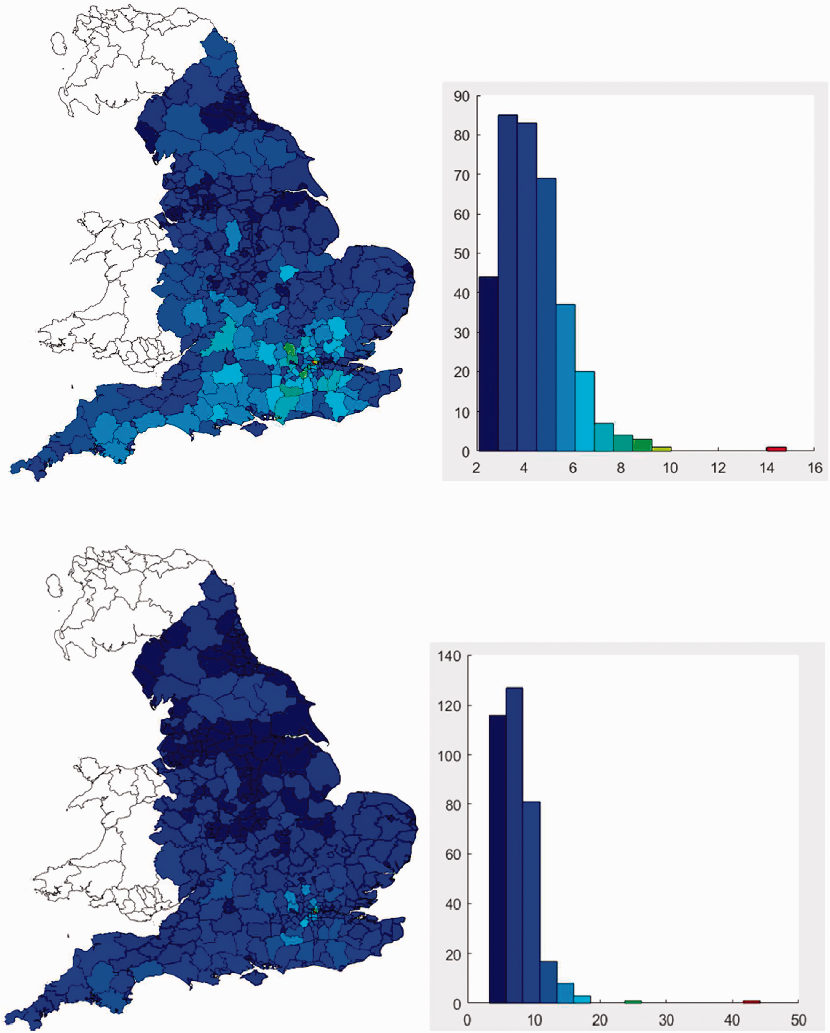
House price to annual wage ratio in 1998 (top) and 2012 (bottom), England.

Table 5.

The effects on prices and affordability in 2012 of a hypothetical 5% increase in supply.

	Counterfactual price		Counterfactual affordability
	Mean	Median	Mean	Median
Both supply and demand effects
Greater London	431,329	372,004	11.49	9.23
England	229,272	206,688	7.50	6.89
Supply effects only
Greater London	428,745	369,197	11.42	9.16
England	228,711	205,886	7.48	6.88

Notes: with supply effects only, counterfactual price series were obtained on the assumption that there was no concomitant increase in the demand for housing, so that $Δ I_{τ}^{c} = 0$ across all districts and $Δ S_{τ} = 0$ outside of Greater London. Elsewhere, within Greater London, $Δ S_{i τ} = 0.05 S_{i τ}$ .

From Figure 1, we can see that the price–wage ratio increased quite dramatically over the period, indicating falling affordability.⁷

Model specification

This section describes the reduced form giving the econometric model specification and gives a brief outline of the estimation methodology leading to the estimates given later in Table 2. These are the basis of the simulation results given later in the paper.

It is easy to show that having normalised the supply function with respect to $p_{i t}$ , that is, rearranging equation (1) with price on the left-hand side, and then substituting for $q_{i t}$ using the demand function of equation (2), the reduced form is

p_{i t} = γ p_{i t - 1} + ρ_{1} \sum_{k = 1}^{N} w_{i k} p_{k t} + β_{1} I_{i t}^{c} + β_{2} S_{i t} + β_{3} B_{t} + β_{4} F_{t} + θ \sum_{k = 1}^{N} w_{i k} p_{k t - 1} + ε_{i t} i = 1, …, N; t = 2, …, T

(3)

We also include random effects $μ_{i}$ taking account of inter-district heterogeneity, and transient effects $ν_{i t}$ picking up spatially and temporally varying shocks, and assume that the disturbances comprise an autoregressive spatial dependence process with the same weights matrix as the spatial lags in equation (3), but with parameter $ρ_{2}$ :

\begin{array}{l} ε_{i t} = ρ_{2} \sum_{k = 1}^{N} m_{i k} ε_{k t} + u_{i t} \\ ε_{t} = (I_{N} - ρ_{2} W_{N}) - 1 u_{t} = H_{N}^{- 1} u_{t} \\ u_{i t} = μ_{i} + ν_{i t} \\ M_{N} = W_{N} an N \times N matrix of known spatial weights \\ I_{N} is an N \times N identity matrix \\ μ_{i} \sim i i d (0, σ_{μ}^{2}) the individual-specific time-invariant effect \\ ν_{i t} \sim i i d (0, σ_{ν}^{2}) the remainder effect \\ cov (μ_{i}, ν_{i t}) = 0 \end{array}

(4)

Baltagi et al. (2014) develop an estimator, with the acronym GMM-SL-SAR-RE,⁸ for an equivalent dynamic spatial panel model with autoregressive spatial disturbances but with $θ$ restricted to zero, which is based on the work of Arellano and Bond (1991) and Mutl (2006), and on the spatial method of moments (GM) estimator proposed by Kapoor et al. (2007). Baltagi et al. (2018) introduce an estimator based on this approach but with $θ$ not restricted to zero, which differs from our estimator in that it assumes a spatial moving average error process for the disturbances. This is the basis of the estimator employed in this paper. We omit much technical detail, but the basic idea is to include both non-spatial and spatial instruments in the estimator to obtain consistent estimates of the parameters. Monte Carlo simulations carried out by Baltagi et al. (2014, 2018) show that for a data-generating process with these characteristics, GMM-SL-SAR-RE is superior to OLS, which ignores the endogeneity of the spatial and temporal lags, the existence of individual effects $μ_{i}$ and the spatial dependence in the disturbances. Likewise, it is preferable to the within- or fixed-effects estimator, which does take care of $μ_{i}$ , but which also does not deal with the endogeneity of the lags or the spatial dependence in the disturbances. Also, the original Arellano and Bond (1991) GMM estimator ignores the spatial process in the disturbances, while the estimator of Mutl (2006) does not include the spatial lag, so these also perform less well than GMM-SL-SAR-RE.

To summarise, following Arellano and Bond (1991) and Baltagi et al. (2014, 2018), we eliminate the individual effects $μ_{i}$ , which are correlated with the spatial lag and temporal lags of the dependent variable, by first differencing the model. Next, again following this literature, moments conditions are created on the basis of an assumption of no correlation between first-differenced disturbances and time-lagged levels of variables. As explained by Bond (2002), the extent of lagging depends on whether variables are considered exogenous, predetermined or endogenous. In this particular application, the variables $I_{t}^{c}$ and $S_{t}$ are assumed to be predetermined, which means they are contemporaneously uncorrelated with the $ν_{i t}$ , but may be correlated with the $ν_{i t - 1}$ and earlier shocks. We therefore assume that prices may feed back and affect income and supply, but this effect is not instantaneous. Following Bond (2002), these predetermined variables are lagged by one period in the construction of moments equations so as to eliminate correlation between the instruments at time $t - 1$ and earlier and $Δ ν_{i t}$ . Likewise, the spatial lags of these variables are also lagged by one period to give an enhanced set of moments equations. Using these instruments in a spatial GM estimator, we obtain consistent estimates of $γ, ρ_{1}, β_{1}, β_{2}, β_{3}, β_{4}, θ$ . The first-differenced residuals provided allow estimation, using non-linear least squares to solve the sample moments, of $ρ_{2}, σ_{ν}^{2}, σ_{μ}^{2}$ based on Kapoor et al. (2007). Finally, again following Arellano and Bond (1991) and Baltagi et al. (2014, 2018), we obtain final estimates of $γ, ρ_{1}, β_{1}, β_{2}, β_{3}, β_{4}, θ$ via a two-step spatial GM estimator. We omit technical detail of the robustness of these estimates, which is available from Baltagi et al. (2014, 2018).

Results

Model estimates

We estimate the model using data for the period 1998–2011, thus omitting the most recent observations for 2015, which are retained to enable one-step ahead predictions. Table 2 gives the resulting parameter estimates, standard errors and t ratios, indicting highly significant temporal and spatial lags, a very strong positive relationship between price and income within commuting distance, and a strong negative relationship between the stock of dwellings and price. There is also positive spatial dependence among the disturbances, but the individual heterogeneity (as measured by the estimated $σ_{μ}^{2}$ ) is comparatively large compared to the variance of the transient effects $({\hat{σ}}_{ν}^{2})$ . According to Elhorst (2001:131), Parent and LeSage (2011: 478, 2012: 731) and Debarsy et al. (2012: 162), the dynamic stability and stationarity of the model requires that

\begin{array}{l} γ + (ρ_{1} + θ) e_{\max} < 1 & and & ρ_{1} + θ \geq 0 \\ γ + (ρ_{1} + θ) e_{\min} < 1 & and & ρ_{1} + θ < 0 \\ γ - (ρ_{1} - θ) e_{\max} > - 1 & and & ρ_{1} - θ \geq 0 \\ γ - (ρ_{1} - θ) e_{\min} > - 1 & and & ρ_{1} - θ < 0 \end{array}

(5)

in which e is a vector of eigenvalues of

W_{N}

. Given

e_{\max} = 1

and

e_{\min} = 0.001

and using the parameter estimates in Table 2, we conclude that the model is stationary.

The one-step-ahead predictions for 2012 were obtained following Chamberlain (1984), Sevestre and Trognon (1996) and Baltagi et al. (2014), who proposed a linear predictor of equation (3) under the assumption that $θ = 0$ . But this also depends on a process that generates initial values that could be impracticable. In this section we give an alternative predictor for the case in which $θ \neq 0$ and which does not depend on the generation of unobserved initial values $p_{0}$ . Following Baltagi et al. (2018), but in the context of spatial autoregressive errors, as a first step we obtain estimates of the individual effects $μ_{i}$ from the residuals averaged over time. Thus, we commence with the equation (3) specification written thus:

\begin{array}{l} p_{t} = ρ_{1} W_{N} p_{t} + β_{1} I_{t}^{c} + β_{2} S_{t} + β_{3} B_{t} + β_{4} F_{t} + C_{N} p_{t - 1} + ε_{t} \\ C_{N} = (γ I_{N} + θ W_{N}) \end{array}

(6)

in which

ρ_{1}, γ, β_{1}, β_{2}, β_{3}, β_{4}

and

θ

are scalar parameters and

I_{N}

is an

N

N

identity matrix. Given the SAR error process based on scalar parameter

ρ_{2}

and thus

H_{N} = (I_{N} - ρ_{2} W_{N})

, this leads to

ε_{t} = H_{N}^{- 1} u_{t} = p_{_{t}} - ρ_{1} W_{N} p_{_{t}} - C_{N} p_{_{t - 1}} - β_{1} I_{t}^{c} - β_{2} S_{t} - β_{3} B_{t} - β_{4} F_{t}

(7)

so that

\begin{array}{l} u_{t} = μ + ν_{t} = H_{N} (p_{_{t}} - ρ_{1} W_{N} p_{_{t}} - C_{N} p_{_{t - 1}} - β_{1} I_{t}^{c} - β_{2} S_{t} - β_{3} B_{t} - β_{4} F) \\ μ = H_{N} (p_{_{t}} - ρ_{1} W_{N} p_{_{t}} - C_{N} p_{_{t - 1}} - β_{1} I_{t}^{c} - β_{2} S_{t} - β_{3} B_{t} - β_{4} F) - ν_{t} \end{array}

(8)

We obtain $\hat{μ}$ by using the N × 1 observed price series $p_{t}$ together with $I_{t}^{c}$ , $S_{t}$ , $B_{t}$ $, F_{t}$ and ${\hat{ρ}}_{1}, \hat{γ}, \hat{θ}, {\hat{β}}_{1}, {\hat{β}}_{2}, {\hat{β}}_{3}, {\hat{β}}_{4}, {\hat{ρ}}_{2}$ , as given in Table 2, and drawing an N × 1 vector $ν_{t}$ from the $N (0, {\hat{σ}}_{ν}^{2})$ distribution to give $\hat{μ}$ for each of $t = 2, … T$ . We take the time mean of these $T - 1$ different estimates, over the years 1998–2011, to give an estimate of the time-constant N × 1 vector $μ$ . We denote this estimate by $\bar{μ}$ .

Given $\bar{μ}$ , we obtain a price prediction for 2012 using the estimates ${\hat{ρ}}_{1}, \hat{γ}, \hat{θ}, {\hat{β}}_{1}, {\hat{β}}_{2}, {\hat{β}}_{3}, {\hat{β}}_{4}, {\hat{ρ}}_{2}$ obtained from data for the period up to 2011 combined with the observations on the explanatory variables for $τ = 2012$ , thus ensuring that the parameter estimates are independent of the 2012 data and providing a valid method for testing the predictive ability of the model. Therefore, predictions are obtained using the prediction equation

\begin{array}{l} {\hat{p}}_{τ} = {\hat{B}}_{N}^{- 1} [{\hat{C}}_{N} p_{τ - 1} + {\hat{β}}_{1} I_{τ}^{c} + {\hat{β}}_{2} S_{τ} + {\hat{β}}_{3} B_{τ} + {\hat{β}}_{4} F_{τ} + {\hat{H}}_{N}^{- 1} \bar{μ}] \\ {\hat{B}}_{N}^{- 1} = (I_{N} - {\hat{ρ}}_{1} W_{N})^{- 1} \\ _{\hat{C}}^{N} = (\hat{γ} I_{N} + \hat{θ} W_{N}) \\ {\hat{H}}_{N}^{- 1} = (I_{N} - {\hat{ρ}}_{2} W_{N})^{- 1} \end{array}

(9)

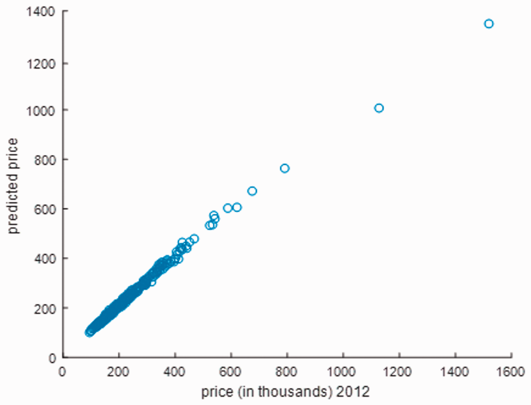
The predicted and actual prices for 2012 for each of $N = 353$ districts are given in Figure 2, and this indicates that the model works quite well for most districts.

Figure 2.

One-step-ahead predictions.

A measure of the relative predictive ability of the model versus various sub-models in which various parameters are restricted to zero is given by the root mean square error (RMSE), where

RMSE= \sqrt{\frac{\sum_{i = 1}^{N} {({\hat{p}}_{τ} - p_{τ})}^{2}}{N}}

(10)

Table 3 shows the loss of fit relative to the predictions given by the full model that occurs when the various model parameters are constrained to zero. An RMSE value similar to that for the full model would indicate that a given restriction was acceptable and make no difference to the predictive performance of the model. However, we find that the RMSEs reflect what is shown by the t ratios in Table 2. While the estimator does not provide a t ratio for $ρ_{2}$ , interestingly, assuming no spatial dependence in the errors ( $ρ_{2} = 0$ ) produces a larger RMSE than nullifying the effect of demand variation.

Simulation methodology

The motivation for our simulation is to try to quantify what effect a localised autonomous increase in the supply of dwellings would have on local and regional house prices and affordability. The approach adopted is to use the parameter estimates given in Table 2 to generate ‘what if’ scenarios – in other words, house prices under an assumption that the number of dwellings was much larger than actually observed in specific locations.⁹ The very small standard errors of the estimated model mean that within the range of variation this allows, the variation in simulation outcome is likely to be small:

{\hat{p}}_{τ} = {\hat{B}}_{N}^{- 1} [{\hat{C}}_{N} p_{τ - 1} + {\hat{β}}_{1} (I_{τ}^{c} + Δ I_{τ}^{c}) + {\hat{β}}_{2} (S_{τ} + Δ S_{τ}) + {\hat{β}}_{3} B_{τ} + {\hat{β}}_{4} F_{τ} + {\hat{H}}_{N}^{- 1} \bar{μ}]

(11)

To obtain the counterfactual price for the year $τ =$ 2012 (for which we have data), counterfactual values for demand and/or supply are utilised, as denoted by $I_{τ}^{c} + Δ I_{τ}^{c}$ and $S_{τ} + Δ S_{τ}$ . Also the 2012 mean bank rate and FTSE index are used for $B_{τ}$ and $F_{τ}$ . Initially, the level of housing supply in each London borough was incremented by 5%, and then by 15%. We also explore the ramifications for prices and affordability on the basis of 1.6 million more homes across Greater London, which on our estimation is an increment of approximately 48% in the stock of homes. Counterfactual price series were obtained on the assumption that there was no concomitant increase in the demand for housing, so that $Δ I_{τ}^{c} = 0$ across all districts and $Δ S_{τ} = 0$ outside of Greater London. Elsewhere, within Greater London, $Δ S_{i τ} = 0.05 S_{i τ}$ and alternatively $Δ S_{i τ} = 0.15 S_{i τ}$ .

In addition, we make the assumption that a higher level of supply would entail higher-level demand as more workers occupy the additional accommodation. In our estimation of the counterfactual level of demand in 2012, we simply utilise wages at their 2012 levels. To obtain the change in income within commuting distance $Δ I_{i τ}^{c}$ , we use essentially the same method used for $I_{i t}^{c}$ , as described earlier. Thus, we need to estimate the increase in income by district, $Δ I_{i τ}$ , which is approximated by the Hadamard product of the N × 1 vector of mean employee wage rate ${\bar{w}}_{τ}$ and the increase in the number of employees working in each district $Δ E_{τ}$ . To obtain the increase in employment level $Δ E_{τ}$ , we calculate the ratio of the total number of workers in England to the total number of dwellings, thus eliminating the effects of commuting. The employment increase $Δ E_{τ}$ is equal to the increase in number of dwellings $Δ S_{τ}$ multiplied by this ratio, which is equal to zero for all but the London boroughs. Thus,

Δ I_{i τ} = {\bar{w}}_{i τ} \circ Δ E_{i τ}

(12)

and this gives

Δ I_{i τ}^{c} = \sum_{k = 1}^{N} {\tilde{C}}_{i k} Δ I_{k τ}

(13)

Simulation results

Figure 3 shows the impact, as given by equation (8), of a hypothetical step increment of 5% in the number of dwellings in each London borough (plus the City of London) on its 2012 level. To interpret Figure 3, districts across the whole of England have been sorted according to the strength of the impact on price.

Figure 3.

Impact of 5% increase in supply on London house prices.

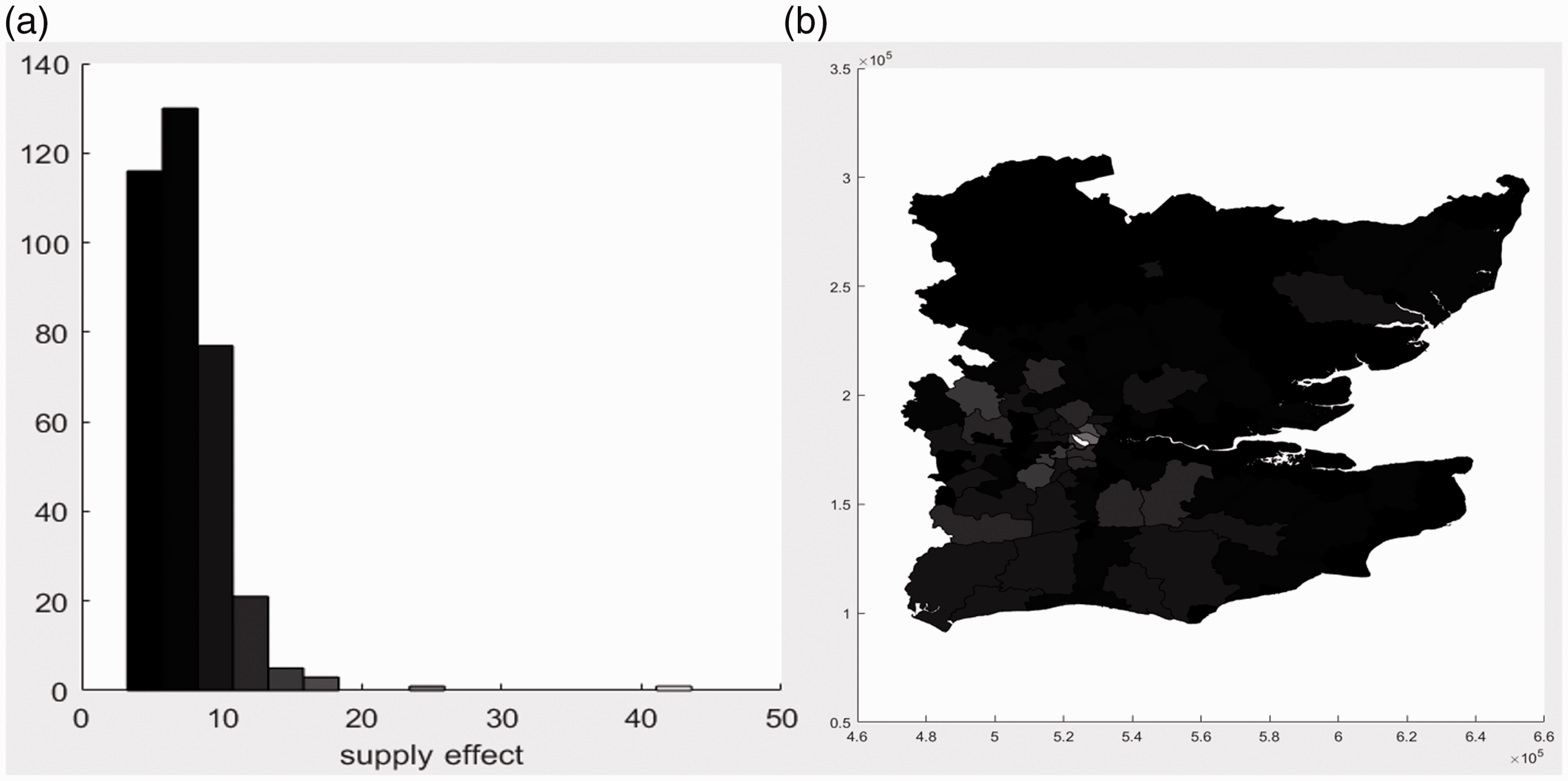
This shows that within Greater London the extra supply of housing produces a fall in price of between about £4000 and £12,000. Many other areas of England see prices fall by less than £4000, but this is in response to an increase in supply confined to Greater London. This is also illustrated by the Figure 4(a) histogram, which gives the distribution of price impacts across all English districts. The Figure 4(b) map focuses on price changes in the South East of England, centred on London, which sees the greatest impact. The darkest shading highlights the London boroughs, but spillover effects are also felt outside the area actually receiving the supply-side stimulus.

Figure 4.

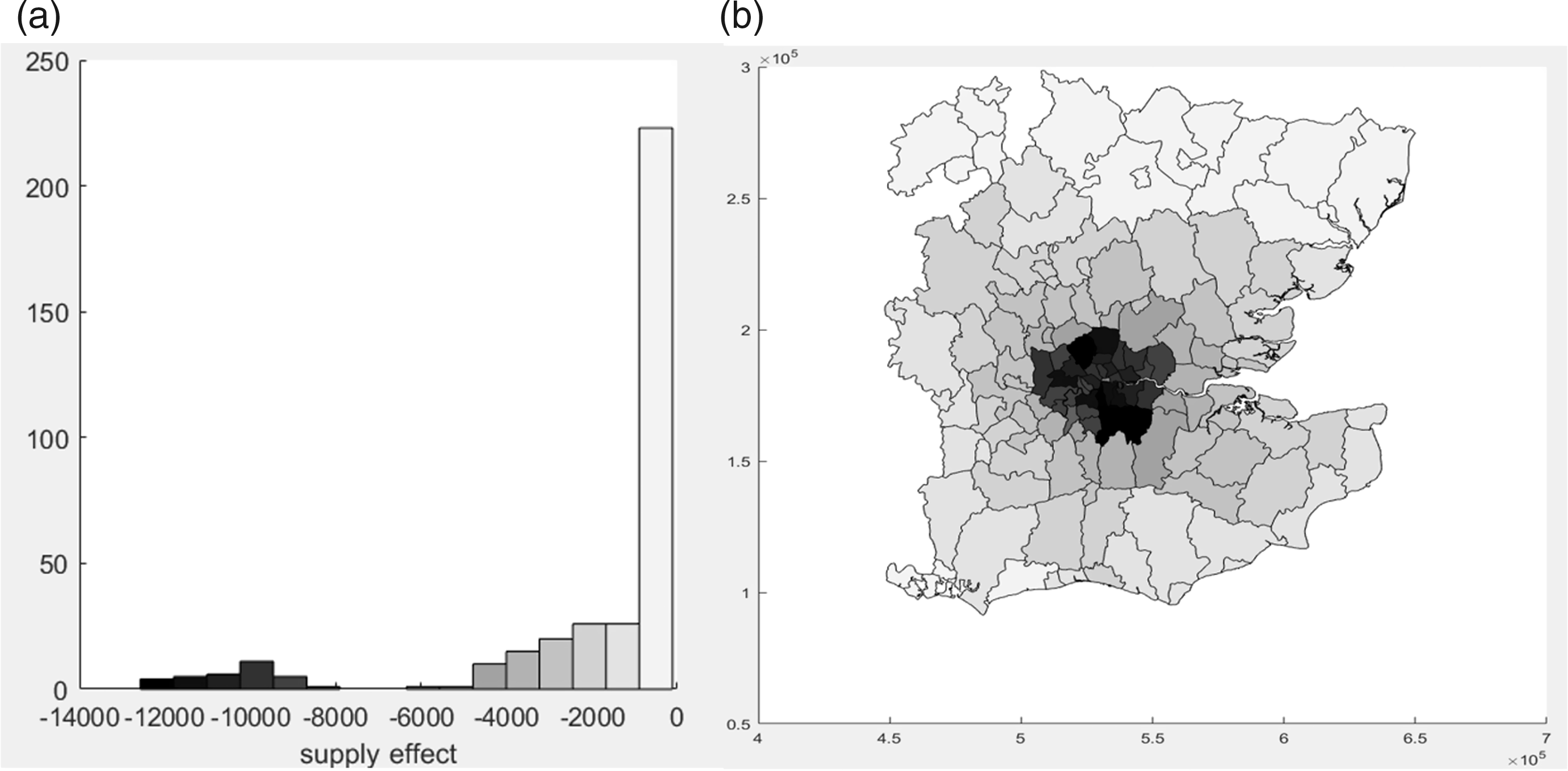
Effect of a 5% increase in the London supply of housing: (a) England; (b) South East England.

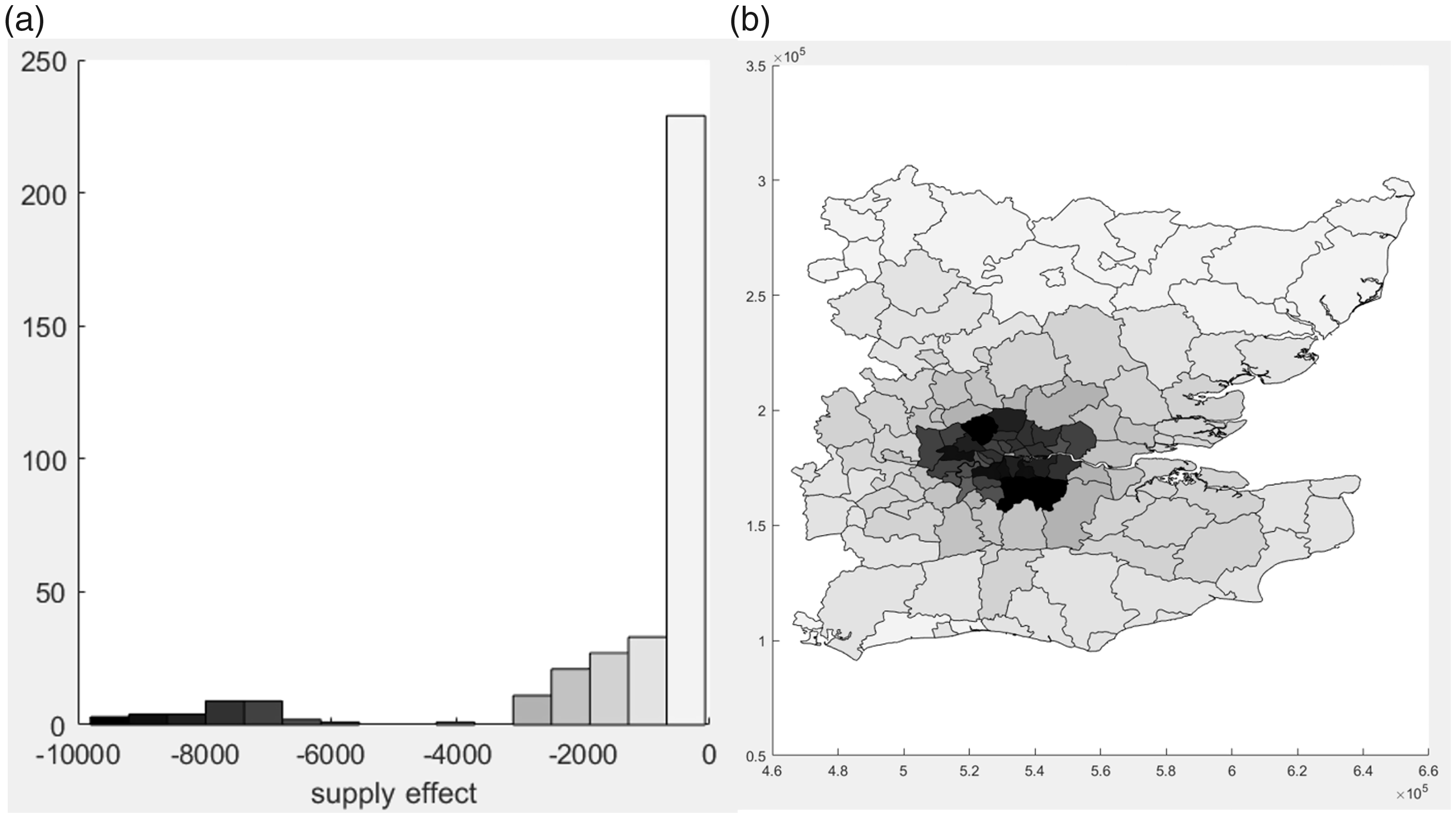
The simulations described in Figure 4 assume that an increase in supply occurs without any concomitant increase in demand. However, demand may change due to the increase in the number of dwellings generating an increase in the labour force and therefore income. Figure 5 shows the increase in price due to the induced increase in demand. Prices would rise by about £2500 in Inner London. Figure 6 gives the net outcome of the negative supply effect plus the positive demand effect, showing that prices fall by about £4000 to £10,000 in the London boroughs, with spillover causing price reductions outside London. Of the 353 English districts, more than 200 do not see any price effect as a result of the increased supply of dwellings in London. Tables 4 and 5 give quantitative details. While price reductions would be the outcome of a 5% increase in supply, the small scale of the effect would make hardly any difference to affordability.

Figure 5.

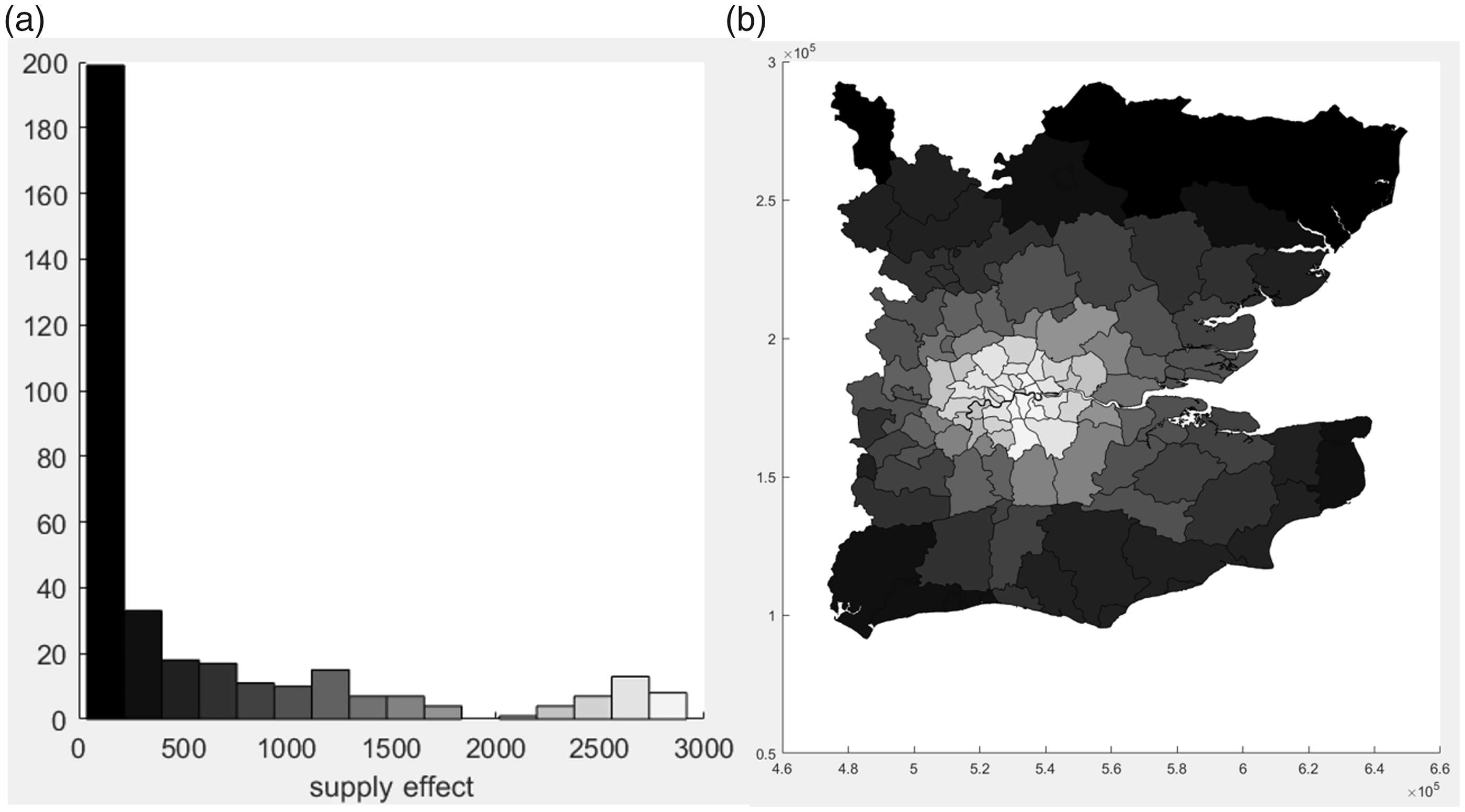
Effect of demand increase due to a 5% increase in the London supply of housing: (a) England; (b) South East England.

Figure 6.

Net effect of 5% increased supply and increased demand: (a) England; (b) South East England.

In order to obtain a greater impact, we increase the existing supply of dwellings by 15%. The resulting figures are similar to Figures 4 –6, so we omit these to save space. The greater increase in supply would cause prices to fall by approximately £30,000 in the London boroughs, but with the spillover effect causing price reduction elsewhere in the South East of England and beyond. Again, assuming that increased numbers of dwellings has a concomitant effect on the number of workers and hence demand, prices would increase by about £8000 in the Inner London boroughs, with the net effect being a price fall of about £22,000 in the London boroughs, with smaller reductions outside Greater London. The summary of effects in Table 6 indicates that a 15% increase in supply in Greater London does make housing more affordable, but not by a large amount, and it fails to eliminate the affordability gap between London and the rest of England. Figure 7 shows the resulting distribution of affordability,¹⁰ assuming both demand and supply effects. A significant aspect of this is the relatively more affordable housing in the Thames estuary, with price–wage ratios of approximately 5. In contrast, Kensington and Chelsea has a ratio in excess of 40, reflecting the special status of this area as a recipient of inward property investment from overseas.

Table 6.

The effects on prices and affordability in 2012 of a hypothetical 15% supply increase.

	Counterfactual price		Counterfactual affordability
	Mean	Median	Mean	Median
Both supply and demand effects
Greater London	416,061	356,791	11.07	8.80
England	226,694	203,724	7.42	6.87
Supply effects only
Greater London	408,307	348,371	10.85	8.60
England	225,012	202,706	7.37	6.81

Figure 7.

Affordability with 15% increased supply. (a) England; (b) South East England.

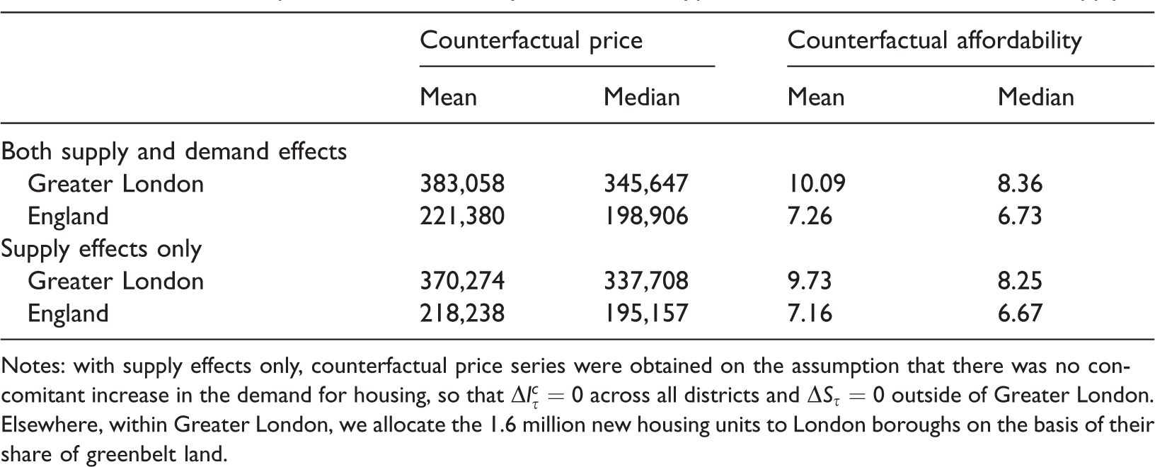
Our final simulation is summarised in Table 7. This is based on the suggestion by Cheshire (2014) that ‘building on greenbelt land would only have to be very modest to provide more than enough land for housing for generations to come: there is enough greenbelt land just within the confines of Greater London – 32,500 hectares – to build 1.6 million houses at average densities’. We put this to the test by estimating what the effect of an extra 1.6 million houses would be, in this case allocating the housing to London boroughs on the basis of their share of greenbelt land. This does have a major impact on affordability, reducing it to a mean of 9.73 and a median value of 8.25. Mean prices would fall by about £70,000. There is a marginal impact when we factor in the effect of increased demand, which raises mean affordability to 10.09 and median affordability to 8.36. These are both significantly below the 2012 mean and median values. Prices in this scenario are on average about £55,000 below what they otherwise would be. It might be supposed that the extra housing would be occupied by many commuters who currently travel in from outside Greater London, but for simplicity we have not adjusted the levels of housing demand downwards in out-of-London districts to allow for a potential exodus of former residents. If this was a large effect, then the lower prices outside of London would to an extent spill over into Greater London itself and could have a further dampening effect on the level of prices and make housing more affordable. Likewise, if the new supply was largely filled by a ‘churning’ of Greater London residents, with Londoners moving out to former greenbelt areas and releasing accommodation elsewhere in the capital, then extra demand in the greenbelt could be to some extent compensated by the spillover effects of reduced demand elsewhere in London. In reality, new housing could be filled by a mix of current London residents, former commuters and migrants from outside the commuting belt or from overseas. The scale of these effects on demand is difficult to assess, but our estimation is that, at best, with zero impact from additional demand, mean affordability would be 9.73, so even with this exceptionally large increase in the provision of housing services in Greater London, affordability is still worse than in England as a whole.

Table 7.

The effects on prices and affordability in 2012 of a hypothetical 1.6 million increase in supply.

	Counterfactual price		Counterfactual affordability
	Mean	Median	Mean	Median
Both supply and demand effects
Greater London	383,058	345,647	10.09	8.36
England	221,380	198,906	7.26	6.73
Supply effects only
Greater London	370,274	337,708	9.73	8.25
England	218,238	195,157	7.16	6.67

Conclusions

Housing affordability has been a key political and economic concern in the UK for a number of years. A lack of new housing supply in high-priced areas is generally mentioned as the main cause of affordability problems. However, this study shows that simply increasing the stock of housing may not be sufficient for reducing prices as the corresponding demand also needs to be considered. Unlike Glaeser et al. (2006), we show that even if wages remain unchanged, new supply can have a much smaller effect on affordability than anticipated. This is mainly due to changes to the size of the local labour force, a factor that has been largely ignored in local and regional housing market forecasts.

Policies that reduce prices effectively are difficult to identify. In fact, even new supply does not appear to be a good way to reduce house prices as the corresponding demand also needs to be considered. Simulation results presented in this study show that improvements in the affordability ratio resulting from new supply are likely to be relatively modest. The key implication for policy makers is that they should carefully consider the interaction between supply and demand when designing and implementing new housing policies.

It is also important to note the effect of commuting patterns on housing markets. In this study, it is assumed that commuting costs will remain as in the Census year 2001. However, they have risen inexorably, up 18% over the last three years. With growing transport costs, it will become increasingly difficult to find substitutes for housing in a particular location. This is likely to increase house prices and reduce affordability. In turn, this would make long-distance commuting more attractive. If so, rising commuting costs are unlikely to reduce demand for it. Instead, the cost of the substitute (housing close to a workplace) is likely to grow accordingly. This shows that increasing commuting costs are likely to lead to lower housing affordability, but not a reduced number of commuters. This has interesting implications for urban sustainability as it suggests that the best way to reduce commuting trips is to improve housing affordability. At the same time, it indicates that reducing transportation costs could help reduce house prices. More research is needed to confirm this logic, but it appears that commuting patterns are closely linked to housing affordability.

Overall, our empirical prediction shows that increasing housing supply appears to have only a weak impact on affordability levels once the spatial dynamic effects of a supply shock are taken into account. Future work might seek to explore this prediction with more extensive empirical data.

Footnotes

Declaration of conflicting interests

The author(s) declared no potential conflicts of interest with respect to the research, authorship and/or publication of this article.

Funding

The author(s) received no financial support for the research, authorship and/or publication of this article.

Notes

Appendix A

References

Arellano

Bond

(1991) Some tests of specification for panel data: Monte Carlo evidence and an application to employment equations. The Review of Economic Studies 58(2): 277–297.

Aslund

Rooth

(2007) Do when and where matter? Initial labour market conditions and immigrant earnings. The Economic Journal 117(518): 422–448.

Ball

Meen

Nygaard

(2010) Housing supply price elasticities revisited: Evidence from international, national, local and company data. Journal of Housing Economics 19(4): 255–268.

Baltagi

Fingleton

Pirotte

(2014) Estimating and forecasting with a dynamic spatial panel data model. Oxford Bulletin of Economics and Statistics 76: 112–136.

Baltagi

Fingleton

Pirotte

(2018) A time–space dynamic panel data model with spatial moving average errors. Regional Science and Urban Economics. Epub ahead of print 9 May 2018. DOI: 10.1016/j.regsciurbeco.2018.04.013.

Barker

(2004) Review of Housing Supply: Delivering Stability – Securing Our Future Housing Needs, Final Report. London: ODPM.

Bernstein

Brocht

Spade-Aguilar

(2000) How Much Is Enough? Basic Family Budgets for Working Families. Washington, DC: Economic Policy Institute.

Bissell

(2014) Transforming commuting mobilities: The memory of practice. Environment and Planning A 46(8): 1946–1965.

Bond

(2002) Dynamic panel data models: A guide to micro data methods and practice. Portuguese Economic Journal 1: 141–162.

10.

Bramley

(1994) An affordability crisis in British housing: Dimensions, causes and policy impact. Housing Studies 9(1): 103–124.

11.

Chamberlain

(1984) Panel data. Handbook of Econometrics 2: 1247–1318.

12.

Cheshire

(2014) Turning houses into gold: The failure of British planning. CentrePiece 19(1): 15–18.

13.

Crook

Burgess

Dunning

et al . (2010) The Incidence, Value and Delivery of Planning Obligations in England in 2007–08. London: DCLG.

14.

Debarsy

Ertur

LeSage

(2012) Interpreting dynamic space–time panel data models. Statistical Methodology 9: 158–171.

15.

Elhorst

(2001) Dynamic models in space and time. Geographical Analysis 33: 119–140.

16.

Eliasson

Lindgren

Westerlund

(2003) Geographical labour mobility: Migration or commuting? Regional Studies 37(8): 827–837.

17.

Fingleton

(2008) Housing supply, housing demand, and affordability. Urban Studies 45(8): 1545–1563.

18.

Gallin

(2006) The long–run relationship between house prices and income: Evidence from local housing markets. Real Estate Economics 34(3): 417–438.

19.

Gibbons

Mourato

Resende

(2014) The amenity value of English nature: A hedonic price approach. Environmental and Resource Economics 57(2): 175–196.

20.

Gibbons

Overman

Resende

(2011) Real earnings disparities in Britain. LSE Working Paper. London School of Economic, UK.

21.

Glaeser

Gyourko

(2003) The impact of building restrictions on housing affordability. Federal Reserve Bank of New York Economic Policy Review 9(2): 21–39.

22.

Glaeser

Gyourko

Saks

(2006) Urban growth and housing supply. Journal of Economic Geography 6(1): 71–89

23.

Goodman

(1988) An econometric model of housing price, permanent income, tenure choice, and housing demand. Journal of Urban Economics 23(3): 327–353.

24.

Gurran

Whitehead

(2011) Planning and affordable housing in Australia and the UK: A comparative perspective. Housing Studies 26(7–8): 1193–1214.

25.

Haynes

(1997) Labor markets and regional transportation improvements: The case of high-speed trains – an introduction and review. The Annals of Regional Science 31(1): 57–76.

26.

Hilber CA and Vermeulen W (2016) The impact of supply constraints on house prices in England. The Economic Journal 126(591): 358–405.

27.

Holly

Pesaran

Yamagata

(2011) The spatial and temporal diffusion of house prices in the UK. Journal of Urban Economics 69(1): 2–23.

28.

Iacoviello

(2005) House prices, borrowing constraints, and monetary policy in the business cycle. American Economic Review 95(3): 739–764.

29.

Kapoor

Kelejian

Prucha

(2007) Panel data models with spatially correlated error components. Journal of Econometrics 140(1): 97–130.

30.

Lambson

McQueen

Slade

(2004) Do out-of-state buyers pay more for real estate? An examination of anchoring-induced bias and search costs. Real Estate Economics 32(1): 85–126.

31.

MacDonald

Taylor

(1993) Regional house prices in Britain: Long-run relationships and short-run dynamics. Scottish Journal of Political Economy 40(1): 43–55.

32.

Malpezzi

(1999) A simple error correction model of house prices. Journal of Housing Economics 8: 27–62.

33.

Meen

(2002) The time-series behavior of house prices: A transatlantic divide? Journal of Housing Economics 11(1): 1–23.

34.

Meen

(2005) On the economics of the Barker review of housing supply. Housing Studies 20(6): 949–971.

35.

Morrison

Monk

(2006) Job–housing mismatch: Affordability crisis in Surrey, South East England. Environment and Planning A 38(6): 1115–1130.

36.

Mulalic

Van Ommeren

Pilegaard

(2014) Wages and commuting: Quasi‐natural experiments’ evidence from firms that relocate. The Economic Journal 124(579): 1086–1105.

37.

Mutl

(2006) Dynamic panel data models with spatially correlated disturbances. PhD Thesis, University of Maryland, College Park, USA.

38.

Nelson

Pendall

Dawkins

et al . (2002) The link between growth management and housing affordability: The academic evidence. Discussion Paper. Brookings Institution Center on Urban and Metropolitan Policy, USA.

39.

Ortalo-Magne F and Rady S (2006) Housing market dynamics: On the contribution of income shocks and credit constraints. The Review of Economic Studies 73(2): 459–485.

40.

Parent

LeSage

(2011) A space–time filter for panel data models containing random effects. Computational Statistics and Data Analysis 55: 475–490.

41.

Parent

LeSage

(2012) Spatial dynamic panel data models with random effects. Regional Science & Urban Economics 42: 727–738.

42.

Roback

(1982) Wages, rents, and the quality of life. Journal of Political Economy 90(4): 1257–1278.

43.

Rosen

(1979) Wage-based indexes of urban quality of life. In: Mieszkowski

Straszheim

(eds) Current Issues in Urban Economics. Baltimore, MD: Johns Hopkins University Press, pp.74–104.

44.

(2015) Immigration and house prices in the UK. The Economic Journal 125(587): 1393–1424.

45.

Sevestre

Trognon

(1996) Dynamic linear models. In: Matyas

Sevestre

(eds) The Econometrics of Panel Data. Dordrecht: Springer, pp.120–144.

46.

Stone

(2006) What is housing affordability? The case for the residual income approach. Housing Policy Debate 17(1): 151–184.

47.

Sultana

(2002) Job/housing imbalance and commuting time in the Atlanta metropolitan area: Exploration of causes of longer commuting time. Urban Geography 23(8): 728–749.

48.

Szumilo

Laszkiewicz

Fuerst

(2017) The spatial impact of employment centres on housing markets. Spatial Economic Analysis 12: 472–491.

49.

Tse

Chan

(2003) Estimating the commuting cost and commuting time property price gradients. Regional Science and Urban Economics 33(6): 745–767.

50.

Weiner

Fuerst

(2017) The dynamics of house prices in Israel and the effect of the investor’s fear gauge. Journal of Housing Research 26(1): 95–117.

51.

White

Allmendinger

(2003) Land-use planning and the housing market: A comparative review of the UK and the USA. Urban Studies 40(5–6): 953–972.

52.

Whitehead

CME. (

2007) Planning policies and affordable housing: England as a successful case study? Housing Studies 22(1): 25–44.