






Abstract
We first provide a critical review of statistical procedures employed in the literature for testing uncertainty in digital terrain analysis, then focus on several aspects of spatial autocorrelation that have been neglected in the analysis of gridded elevation data. When applied to first derivatives of elevation such as topographic slope, a spatial approach using Moran’s I and the LISA (Local Indicator of Spatial Association) allows: (1) georeferenced data patterns to be generated; (2) error hot- and coldspots to be located; and (3) error propagation during DEM manipulation to be evaluated. In a worked example focusing on the Wasatch mountain front, Utah, we analyse the relative advantages of six DEMs resulting from different acquisition modes (airborne, optical, radar, or composite): the LiDAR (2 m), CODEM (5 m), NED10 (10 m), ASTER DEM (15 m) and GDEM (30 m), and SRTM (90 m). The example shows that (apart from the LiDAR) the NED10, which is generated from composite data sources, is the least error-ridden DEM for that region. Knowing error magnitudes and where errors are located determines where corrections to elevation are required in order to minimize error accumulation or propagation, and clarifies how they might affect expert judgement in environmental decisions. Ground resolution issues can subsequently be addressed with greater confidence by resampling the preferred grid to terrain resolutions suited to the landscape attributes of interest. Source product testing is an essential yet often neglected part of DEM analysis, with many practical applications in hydrological modelling, for predictions of slope- to catchment-scale mass sediment flux, or for the assessment of slope stability thresholds.
I Introduction
The advent of remote sensing technologies has meant that larger areas can be mapped by fewer people in less time and at diminishing cost (Smith and Clark, 2005). The widespread use of digital elevation models (DEMs) is a direct consequence of those advantages. Traditional methods such as field surveying and photogrammetry can yield high accuracy terrain data, but they are time consuming and labour intensive (Liu, 2008). As a result, DEMs have become the most common method for extracting topographic information, also allowing the flow of water across topography to be analysed, with many practical applications in hydrological modelling and for predictions of slope- to catchment-scale mass sediment flux (Desmet and Govers, 1995; Dietrich et al., 1993; Kamp et al., 2003; Kirkby, 1990). Topographic information in a DEM can be represented and stored as: (1) a triangulated irregular network (TIN); (2) discrete landform elements based on the intersection of flow- and contour lines; or (3) a grid. Here we examine gridded DEMs, which despite drawbacks arising from higher demands on computer memory (Claessens et al., 2005: 462; Yue et al., 2007: 161) nevertheless remain the most commonly used data source for digital terrain analysis because of their simple structure and compatibility with other digitally produced data (Wise, 2000: 1910).
Slope gradient and aspect, which are examined in this review, are two of the most basic parameters affecting landscape-scale natural processes. The accuracy of a slope map determines many of the predictions that geomorphologists, engineers, hydrologists, and ecologists, farmers or foresters make about the behaviour of environmental variables, about natural hazards, land-use potential, and for planning. Errors on slope propagate to more sophisticated DEM-derived terrain attributes such as slope curvature, drainage networks, slope channel lengths, slope widths or topographic wetness indices. Although seemingly obvious, the consideration of error distribution and error propagation in DEMs has nonetheless been neglected in routine DEM-based terrain studies, perhaps because the appeal and immediacy of DEM implementation in commonly available software packages overrides any concern for accuracy and error. The imperfections of gridded DEMs, i.e. the fidelity with which they represent the ‘real world’, have been extensively explored in the last decades. Fisher and Tate (2006) have described errors on gridded data sets as the difference between a model value and the true value, i.e. as deviations from reality (called incorrect elevation values, misplaced elevation values, data gaps, or missing values). True or real values are absolute elevation measurements collected on the Earth’s surface with the instruments of terrestrial geodesy, whether satellite-assisted or not. Like all numerical models (Dietrich et al., 2003: 109–110), elevation models are approximations of reality, but this does not mean that sources of error are unknowable, intractable or unquantifiable. Any step in DEM production could be a source of error, and error should be detected early in the batch processes in order to avoid its insidious propagation to subsequent steps and its effects on the quality of the final product (Darnell et al., 2008; Hengl et al., 2010).
The risk of introducing or ignoring distortions is to generate bias in DEM-based quantitative analyses of the Earth’s surface and in the accurate characterization of landforms and processes. The use of terrain models for environmental and engineering applications, or even for heuristic purposes, thus calls for an assessment of error relating to data type, data precision, the way the data acquisition tools operate, and to the comparative advantages of high ground-resolution (g.r.) data such as LiDAR, SpotLight (g.r.: 1 m, TerraSarX), Cosmo-SkyMed 4 (g.r.: 2–4 m) or Alos Prism (g.r.: 2.5 m) (Hengl et al., 2010: 769). At a time when the number and diversity of satellite, airborne and radar platforms is on the increase due to the rapidly evolving technology, this requires at least some knowledge of data processing techniques and appropriate means for meaningfully evaluating the reliability of results used in terrain analysis.
Here we review the variety and relative performance of existing approaches while emphasizing from the start that few studies have embraced the analysis of spatial autocorrelation as a prerequisite for developing error models. Only random patterns exhibit no spatial autocorrelation (Hunter and Goodchild, 1997; Oksanen and Sarjakoski, 2005). DEM error, however, is in essence already spatially dependent because of the interpolation methods used in DEM generation (Carlisle, 2005: 524; Liu and Bian, 2008: 308). This means that redundancy occurs in spatial data and can bias the common assumptions of independence between values in many statistical operations (e.g. least-squares regression analysis). A review of the techniques and applications of spatial autocorrelation to DEM analysis will accordingly occupy the later sections of this paper and will focus around a worked example providing new results for illustrative and didactic purposes. Some recent studies have addressed spatial autocorrelation as a means of calibrating error models, but have exclusively dealt with global autocorrelation rather than with examining patterns of local-scale variation (Hebeler and Purves, 2009; Lindsay and Evans, 2008; Liu and Bian, 2008; Wechsler and Kroll, 2006), and have tended to focus on global data (e.g. GTOPO30, SRTM: Holmes et al., 2000, Wechsler, 1999; Wechsler and Kroll, 2006) and on the interpolation of high accuracy data (e.g. LiDAR: Arrell et al., 2008). Limited attention has been paid to: (1) the potential for analysing local and global spatial autocorrelation conjointly; (2) the generation of continuous spatial representations of error arising from DEM analysis; and (3) the comparative sensitivity to error of DEMs obtained from different sensors (optical, radar, airborne). We will show how local spatial autocorrelation analysis helps to locate the weaknesses of DEM structure, how it highlights the spatial heterogeneity of error, and how, from the use of local indices, it is possible to obtain error maps useful to a wide range of terrain applications relevant to physical geography.
Accordingly, we will focus on three issues that arise when different DEM sources are available for a given geographical area. (1) How can the accuracy of elevation data be assessed in such situations? (2) How can errors affecting primary topographic attributes such as topographic slope be evaluated, and what confidence can be attributed to such data for hydrological or geomorphometric applications? (3) What error mapping techniques are most advantageous for detecting regions susceptible to error propagation and for visually displaying bias in DEM-based scientific predictions? We first present a review of current knowledge about DEM accuracy and the tracking of error propagation in grid processing. The Local Indicator of Spatial Association (LISA: Anselin, 1995), similar to calculating neighbourhood filters in raster analysis, is then introduced and tested as an illustration of how to select the most efficient error model based on clustering results.
We test six DEM grids obtained from different categories of sensors and focus on techniques for mapping the spatial distribution of error affecting topographic slope values. The chosen study area is the Wasatch mountain front, Utah, USA. The data sources are a LiDAR grid, i.e. an airborne source; the composite CODEM, NED10 and GDEM, each compiled from multiple data sources, i.e. maps and/or optical and/or radar; the ASTER DEM (AstD), an optical source; and the SRTM, a radar source. Each possesses initial statistical characteristics relating to the elevation interpolation procedures, to the error corrections relating to physical acquisition parameters, and to altimetric configurations imposed by the initial choice of geoid reference frame. Although the ground resolutions of the DEMs analysed also happen to range from 2 m to 90 m, what we test here is the quality of the initial products. Ground resolution remains a separate issue. Although the complexity of any land surface is likely to decrease with increasing cell size, with ground resolution potentially affecting error distribution as a consequence, the first step in digital terrain analysis still involves choosing among an increasingly wide range of imperfect digital products, whether these are readily available on the market or purpose-generated by stereo-photogrammetry. Whatever the original ground resolution of the digital product, it becomes advantageous to resample or degrade the DEM to the ground resolution best suited to the application required only after quality checks, such as those proposed in this paper, have been performed. After the most satisfactory digital product available has been selected in this way, work on terrain roughness indices, which measure the variability of elevation based on a sliding window specific to each DEM (Grohmann et al., 2009), is one way of addressing the effects of scale on the analytical accuracy affecting the landscape attributes of interest.
II Evaluation of accuracy and error propagation in gridded DEM processing
According to Hunter and Goodchild (1997: 36), the notion of uncertainty covers undefined error (i.e. when a true value is unknown) and structural error. Undefined error covers a range of subcategories defined by Thapa and Bossler (1992: 836), including blunders, gross errors and systematic errors (see Appendix). Often these cannot be removed, whether by repeated observation or by recourse to a deterministic search function, because they tend to evade any clearly detectable pattern. After Burrough (1986) and Wise (1998), Wechsler (1999: 3) has identified three possible sources of structural error: (1) errors due to an incomplete density of observations, or to consequences of spatial sampling; (2) measurement errors such as positional inaccuracy, which might arise from improper orientation of the stereo-model or by neglecting lens distortion in photogrammetric procedures; and (3) random errors, which can normally be detected after removal of gross and systematic errors (see Appendix) and might be due to data entry faults, observer bias, or computer-generated numerical errors, interpolation errors, or problems of classification and generalization.
Finer differentiation among structural errors distinguishes between horizontal (positional accuracy) and vertical components (attributes accuracy), respectively. These may be difficult to separate (Ehlschlaeger and Shortridge, 1996) but an expression both in terms of the metric accuracy of elevation and in terms of planimetric deviation values is possible (Arrell et al., 2008: 945). Planimetric and metric accuracy have long been evaluated and calculated from routine statistical methods such as mean error (ME), mean absolute error (MAE), error in standard deviation units (S), or as the RMSE, which is the square root of the variance of a distribution (e.g. Carlisle, 2005: 522; Erdogan, 2010; Fisher and Tate, 2006: 470; Wechsler and Kroll, 2006: 1082; see Appendix). Within that class of statistical test, RMSE-based comparison of DEM elevation values with sample values from another, more accurate source seems to be the most appropriate way of providing error estimation (e.g. Arrell et al., 2008: 945; Hirano et al., 2003; Wise, 2007: 1353). However, a major drawback of the RMSE is that results merely provide one global value per DEM grid, i.e. they ignore the finer-scale spatial variability of the error (Wechsler, 2003: 58) that often contains a great deal of useful information for terrain-based applications. Global indices are thus insufficient (Li and Wong, 2010: 252) and any useful study of DEM accuracy should also investigate the spatial variation of error values (Carlisle, 2005: 523; Wood, 1994).
Methods of error investigation in DEMs have been widely explored (Fisher and Tate, 2006; Giles and Franklin, 1996: 1165; Wechsler, 2003: 58; Wilson and Gallant, 2000: 15). The simplest methods are based on criteria such as: (1) differences in elevation between adjacent points (e.g. Binh and Thuy, 2008; Hannah, 1981); (2) systematic detection by inspection of anomalous values within a given moving window (e.g. Chaplot et al., 2006; Felicísimo, 1994; Zhou and Liu, 2004b); (3) the minimization of total error, which is the sum of errors originating from the input data sources and operational errors generated by data manipulation (e.g. Walsh et al., 1987; Younan et al., 2002); or (4) spectral (e.g. Tempfli, 1980) and elevation histogram analyses (e.g. Carrara et al., 1997; Holmes et al., 2000), which each focus on the detection of structure in the statistical distribution of elevation values and on the identification of unexpected variations interpreted as indicating systematic or isolated error. More complex methods introduce remote sensing and/or geostatistical processes. Goodchild (1982) and Polidori (1991: 12–20) have investigated the value of Brownian processes in a fractal terrain simulation model for improving DEM accuracy. Brown and Bara (1994) used semi-variogram and fractal dimension to describe the pattern of systematic errors. López (1997, 2000) developed a method based on principal component analysis (PCA) to locate random errors in DEMs and to extract uncorrelated patterns. After comparisons between Felicisimo’s method (1994) and López’s method (López, 1997), López (2000) revised the PCA approach in order to handle the significant spatial autocorrelation observed in the data. By identifying gross and random errors, systematic errors were avoided. Finally, Arrell et al. (2008) identified and removed artifacts associated with gross error using Fast Fourier Transform analysis as a means of discriminating between signal and noise.
Techniques of error location and visualization have also been considered. Fisher and Tate (2006) have reviewed research in this domain and noted that DEM contour maps could be a useful tool for error observation, with the possibility of detecting gross errors and blunders. The reliability of this method, however, is not proven. The method of Hunter and Goodchild (1995) based on the use of the RMSE as a threshold criterion for testing the accuracy of elevation appears more useful. Other more sophisticated methods have focused on error visualization by using TIN or discrete data and by displaying in 3-D the magnitude of local differences and curvature errors from contoured DEM data (Gousie, 2005). Perhaps a more workable method, proposed by Oksanen (2003: 2412), detects and visualizes gross errors in gridded DEMs from relief shading because of its ability to render a 3-D effect on elevation data. Wise (2007: 1352) has argued that visualization techniques used in error identification could also be efficient at demonstrating strong links between error patterns and interpolation-related distortions. Wood (1996: 64) demonstrated this by developing a spline-fitting algorithm on a fractal surface that allowed errors and other impacts of the algorithmic process to be detected and visually displayed. More recent attention has been paid to DEM interpolation algorithms and their error-causing impacts (1) on elevation in the case of high g.r. data (e.g. LiDAR: Arrell et al., 2008: 944; Bater and Coops, 2009; Lindsay and Evans, 2008; Liu, 2008), (2) on the calculation of mathematical derivatives of elevation (e.g. Florinsky, 1998; Jones, 1998; Liu and Bian, 2008; Schmidt et al., 2003; Zhou and Liu, 2004a), but also (3) on flow simulation and its repercussions on drainage network extraction (e.g. Li and Wong, 2010; Lindsay and Evans, 2008).
In terrain analysis, error propagation analyses have usually focused on slope and aspect as test variables. These mathematical derivatives of elevation are recognized to provide a more useful test of error location and propagation, and thus for DEM quality assessment, than elevation itself because of their greater sensitivity to error (Wechsler, 2003; Wise, 2000: 1911). Liu and Jezek (1999: 250) have listed three approaches for treating the propagation of DEM error. These include empirical approaches (e.g. Bolstad and Stowe, 1994; Gatziolis and Fried, 2004; Lindsay, 2006), analytical methods (e.g. Florinsky, 1998; Heuvelink et al., 1989; Leick, 1990; Oksanen and Sarjakoski, 2005) and computer simulations (e.g. Canters et al., 2002; Ehlschlaeger, 1998; Hebeler and Purves, 2009; Oksanen and Sarjakoski, 2005; Wechsler and Kroll, 2006). (1) The empirical approaches rely on a derivation of the spatial properties of error based on a more accurate reference data set, where results for a series of simulations are presented with error fields characterized by a range of spatial properties (Lindsay and Evans, 2008: 1590). This compensates for the often unknown spatial characteristics of error. (2) Analytical methods can involve Taylor series expansion (Heuvelink et al., 1989). Under the assumption that error distribution follows a Gaussian distribution, this approach constitutes the basis for least-squares adjustment techniques (Hunter and Goodchild, 1997: 36). (3) The simulation methods involve stochastic approaches such as Monte Carlo techniques. This requires a number of equally probable outcomes upon which selected statistics are performed. Uncertainty is quantified by evaluating the statistics associated with the range of outputs under the assumption of spatial autocorrelation. A series of random equiprobable error maps, one of which could be the ‘true’ error map, is provided. Such simulations, however, are non-unique and do not ensure that the true error map has been generated by the procedure (Wechsler, 2006: 2360; Wechsler and Kroll, 2006).
The analytical treatment of terrain algorithms is complicated and laborious (Lindsay and Evans, 2008: 1590). Oksanen and Sarjakoski (2005) confronted an analytical approach with Monte Carlo simulations to evaluate the propagation of error in slope and aspect simultaneously. They concluded that the two methods produced similar results even though the data had not been inspected for spatial autocorrelation in the analytical approach. The work of Oksanen and Sarjakoski (2005: 1016) and Liu and Bian (2008: 308) has revived a debate about the value of performing analytical manipulations of gridded DEMs that disregard the spatial autocorrelation of error — the most important consideration being the choice of autocorrelation parameter rather than the shape of the spatial autocorrelation. These aspects are presently examined.
III Spatial autocorrelation and the production of error maps
Spatial autocorrelation characterizes the correlation between a variable and itself (univariate autocorrelation), or between that same variable and another variable’s values (bivariate autocorrelation), in neighbouring cells. Spatial autocorrelation functions are used to quantify the spatial regularity of a phenomenon (a form of spatial complexity) (Aubry and Piégay, 2001). It is based on the assumption that in all data sets near things are more related than distant things (Tobler’s first law of geography). Some approaches avoid the condition of heteroscedasticity, i.e. the necessity to consider variations in error value as a function of variations in another variable. This occurs in the case of spatial autoregressive models (e.g. Hunter and Goodchild, 1997) and of semi-variance analysis (e.g. Carlisle, 2005; Giles and Franklin, 1996). Other approaches, such as pixel swapping and spatial moving averages using low-pass filters (e.g. Fisher, 1998; Wechsler, 2006), introduce spatial correlation without explicitly addressing error patterns or mapping error surfaces (Hebeler and Purves, 2009: 6). Methods such as sequential Gaussian simulation (e.g. Oksanen and Sarjakoski, 2005) use global spatial autocorrelation information without examining the finer structure of the error. Given that the study of spatial autocorrelation and of its potential consequences in gridded DEMs has been unsystematic, here we investigate the definitions of spatial autocorrelation, its uses, how to deal with it, and how error maps displaying local autocorrelation clusters can reveal error propagation phenomena.
Moran’s I (Moran, 1950) is historically the first index to have been used for understanding spatial autocorrelation, and still a standard. In the context of gridded DEMs, Moran’s I is a global indicator of spatial association and is used to measure average deviations in slope or elevation for an entire grid. This global measure is given by the following formula:
From this index Anselin (1995) later elaborated the LISA, which can also be used on continuous DEM grid surfaces. Here we use Moran’s I and LISA as techniques for visualizing error propagation, and for adding information about spatial autocorrelation not provided by Moran’s I. LISA is used for estimating the local contribution of each pixel value to the global index. Local indicators are based on a gamma statistic (Getis, 1991) given by the following formula (Oliveau, 2005):
Bivariate LISA-type cluster analysis explores the spatial distribution of DEM errors affecting elevation and measures its transmission to errors affecting slope gradient. It follows a scheme of pattern recognition (Jacquez, 2008: 400) made up of five components: (1) a null hypothesis, H0 , which describes the spatial pattern expected when the alternative hypothesis is false (i.e. an absence of significant clustering of errors in slope at sites where errors in elevation occur); (2) an alternative hypothesis, HA , which states that the clustering of errors in slope closely matches the spatial distribution of errors in elevation; (3) a statistical significance test that quantifies the spatial pattern of the data; (4) a neutral spatial model, which is a numerical device for generating the reference distribution based on a Monte Carlo simulation (achieves randomly operated permutations of values); (5) a reference distribution, which is the distribution of the statistical test scores when the null hypothesis is true, and is set by the p-values, which in statistics measure strength of evidence. For the LISA tests, pseudo p-values are computed as (m+1) / (r+1), where r is the number of replications and m is the number of instances where a statistic computed from the permutations is either equal to or greater than the observed value (in the case of positive LISA scores), or equal to or smaller than the observed value (for negative LISA scores) (Anselin, 1995). Results are filtered with the choice of an arbitrary significance threshold, α (0.05, 0.01, 0.001, or 0.0001), which determines confidence intervals used for assessing results.
IV Patterns of error in gridded DEMs: a worked example from the Wasatch Mountains, Utah, USA
Among the few existing studies to have explored the local structure of spatial autocorrelation in raster analysis, Goovaerts et al. (2005) detected anomalies on high-resolution hyperspectral imagery while testing the significance of LISA values through randomization. Erdogan (2010) investigated spatial variation as well as spatial associations of error by comparing a range of interpolation methods. Monckton (1994) used Moran’s I to simulate the spatial structure of error in elevation data. Results, however, were inconclusive, probably because of the spatial lags (which exceeded 250 m) that were used in dealing with spot heights on Ordnance Survey maps (Carlisle, 2005: 524).
In the following worked example designed to illustrate the power of autocorrelation analysis as a tool in DEM error evaluation, we performed tests on a ~29 km2 study area encompassing part of the Weber Segment, one of the longest (61 km) and seismically most active segments of the Wasatch normal fault in Utah (Figure 1). On this segment, faceted spurs and their triangular mountain-front hillslopes are well preserved (McCalpin and Berry, 1996; Nelson and Personius, 1993; Petit et al., 2009; Zuchiewicz and McCalpin, 2000). The geomorphology of fault-generated range fronts is reflected in the drainage basin morphology as well as in the faceted spur geometry. In order to extract precise terrain parameters with minimal bias, DEM evaluation was examined through slope analysis. Using both LISA and Moran’s I, the methodology aims to single out the DEM best suited to geomorphometric or hydrological applications. The best DEM should provide the model with the smallest error, i.e. with the highest accuracy and the lowest level of error clustering.

The Weber Segment in the Wasatch Mountains, Utah, USA. Elevations range from 257 m to 3618 m. The 2-D and 2.5-D views highlight the active normal boundary fault with its triangular faceted spurs.
The grid characteristics of the six DEMs available for the study area (see Introduction), with differing column and row grid-cell sizes, are as follows (Figure 2) – LiDAR (2 m): 2979 × 2370; CODEM (5 m): 1260 × 857; NED10 (10 m): 630 × 474; AstD (15 m): 420 × 316; GDEM (30 m): 210 × 857; SRTM (90 m): 70 × 53. General statistics are usually available for each DEM from supporting documentation, in which major errors and correction processes are mentioned. Out of the six in this study, only the AstD was generated directly from raw data by the authors using digital stereo-photogrammetric techniques summarized in Figure 3. The operational error we use is the difference between the z values provided by each of the five tested DEM grids on the one hand, and the z values provided by the LiDAR data on the other, the latter being closest to any ‘true’ elevation measurement. Any observed difference in z is interpreted as being due to one or several of the error categories defined in the Appendix. Those refer to the various defects originally present in the gridded elevation data. Their distribution pattern across the grid remains unknown until we proceed to the mapping techniques proposed later in this worked example. They depend on the type of sensor from which the data was collected, and how this data was preprocessed before making it available for use by geographers.
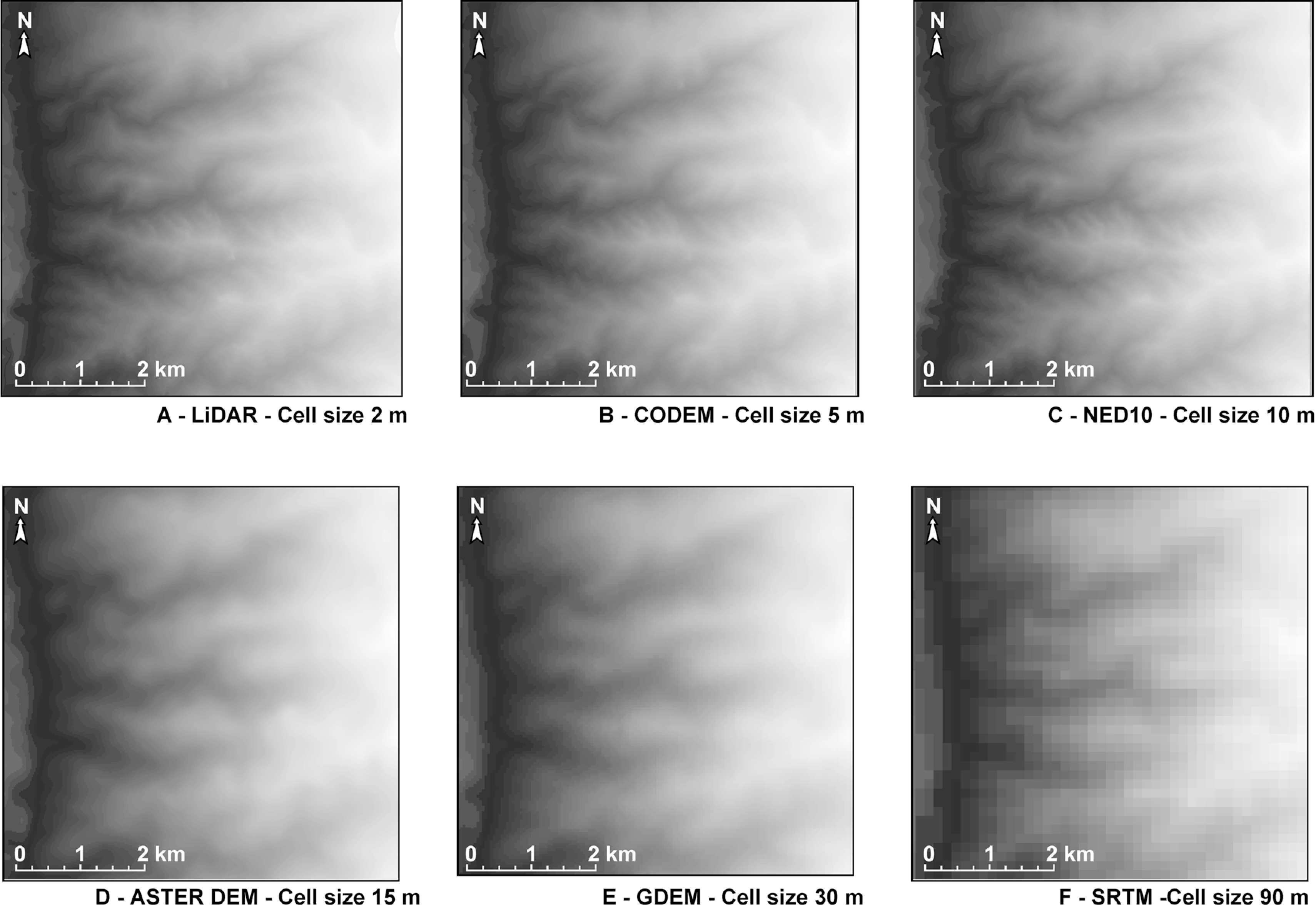
Extract of each studied DEM representing the different grid-cell sizes used in the worked example. (A) LiDAR data (2 m, available at http://gis.utah.gov/elevation-terrain-data/2-meter-bare-earth-lidar). (B) CODEM (5 m, http://gis.utah.gov/elevation-terrain-data/5-meter-auto-correlated-elevation-model-dem). (C) NED10 (10 m, http://gis.utah.gov/elevation-terrain-data/national-elevation-dataset-ned). (D) ASTER DEM (15 m, http://www.echo.nasa.gov/reference/astergdem_tutorial.htm). (E) GDEM (30 m http://asterweb.jpl.nasa.gov/gdem.asp). (F) Shuttle Radar Topography Mission, or SRTM (1 arc second, i.e. ~90 m, http://www.cgiar-csi.org/data/elevation/item/45-srtm-90m-digital-elevation-database-v41).
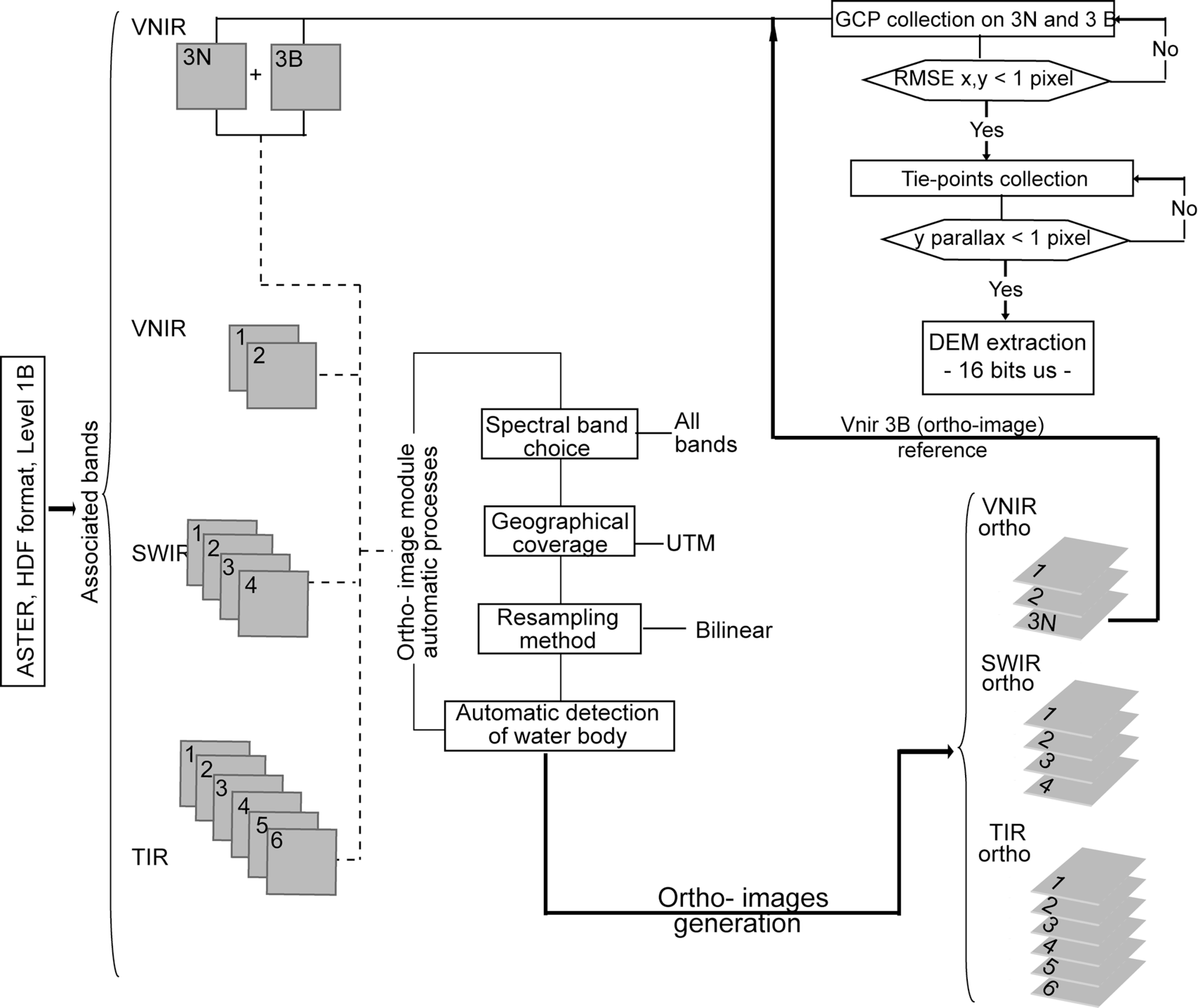
Flow chart explaining the ASTER DEM extraction process from the stereoscopic VNIR 3N and VNIR 3B bands. VNIR: visible near-infrared bands; SWIR: short-wave infrared bands; TIR: thermal infrared bands. VNIR, SWIR and TIR are ortho-rectified bands (geometric corrections). GCP are ground control points extracted from the ortho-rectified VNIR bands. The RMSE is calculated for the (x,y) plane coordinates and the vertical plane z.
1 Vertical accuracy
The first approach to error estimation relied on the RMSE, which integrates errors relating to interpolation methods and to geographical position in x, y and z. Vertical accuracy assessment at pixel scale was first calculated from the LiDAR model (RMSE ≈ 0.086 m) with a regular sample extraction interval of 100 m, each point extracted (3000 for each DEM) being a substitute for ground GPS information (see Appendix for details). Given that, for comparison purposes, the grids could not be used with their original characteristics, DEM resampling was also necessary. Accordingly, for the RMSE calculation resampling procedures were performed on each DEM by transforming cell size to the reference size, i.e. 2 m. To avoid stair-stepping and jagged artifacts in the resampling process, a bicubic spline resampling method was used instead (see Appendix) (Keys, 1981). The resampled grids were used for a comparative assessment of vertical accuracy between DEMs. In order to obtain percent values of transformation from the resampled DEM, a new RMSE value, noted RMSEc, was calculated. The formulae given in the Appendix were applied to the entire DEM grid and assessment of the vertical accuracy of surface objects was carried out using the RMSEc criterion.
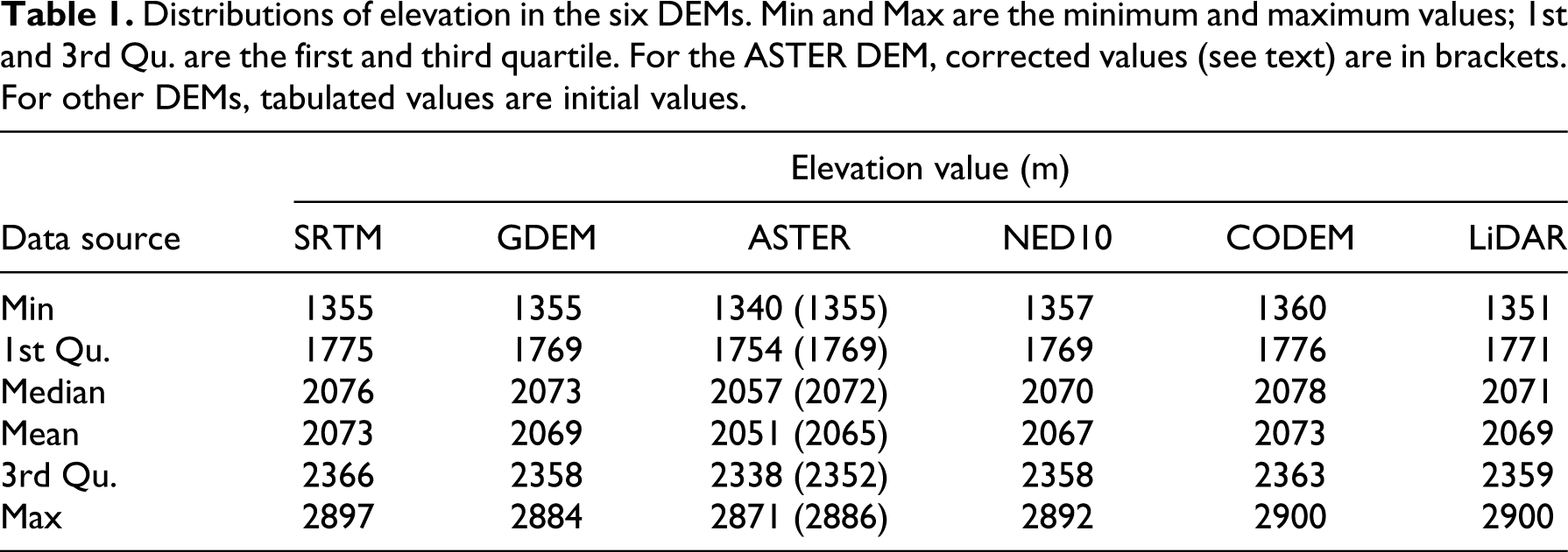
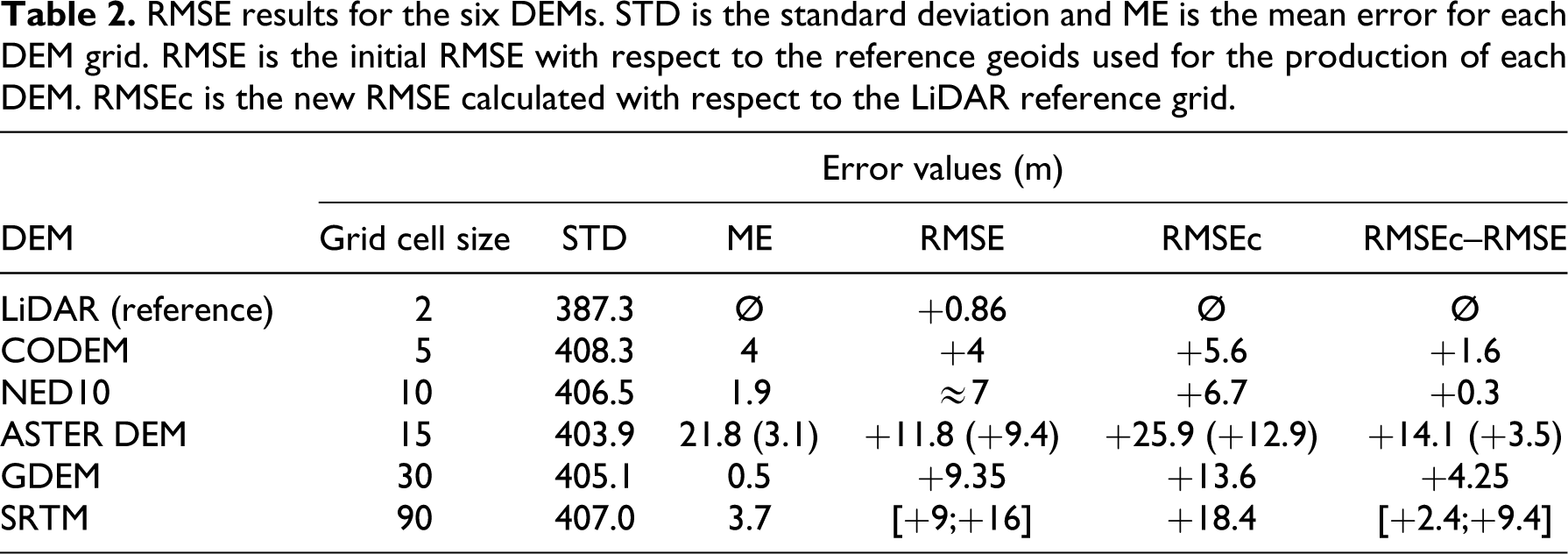
Figure 4 and Table 1 illustrate the distribution of error values in elevation among the six DEM grids. Quartile distributions (first and third) describe a band of ±8 m for minimum and ±22 m for maximum deviations from the mean elevation (Table 2). Overall, DEM height distributions exhibit a similar pattern despite the fact that the elevation sources are different (i.e. airborne, radar, optical or compilation data). The more outstanding exception is the AstD, which presents significant offsets with respect to the other DEMs. These offsets attain a difference in values of about ±15 m (roughly equivalent to one AstD pixel) for height and RMSE measurements as well as for statistical moments. This exception is ascribable to the initial AstD extraction process, in which the precision of the DEM tools used was greater than half a pixel (see Figure 3). The initial RMSE for the AstD (11.8 m) was accordingly too large. The global RMSE should be about half a pixel (7.5 m). Additional ground control points were checked in order to newly interpolate the AstD, finally providing it with elevation ranges similar to the other DEMs, i.e. [1355–1298 m]. As a result, the new value obtained for the AstD RMSEc (Table 2) fell into line with the overall RMSEc trend for the other DEMs, i.e. about 12.9 m. Thus RMSEc results (incorporating new values given in brackets for the AstD) yield results similar to those obtained for the other DEMs: the larger the grid cell size, the higher the RMSEc [+5.7; +18.4] and RMSE [+4; +16 m]. The key conclusion at this stage is that whatever the DEM’s data source, DEM generation does not produce large errors in z. Values for the SRTM and GDEM also fall close to the reference LiDAR value and thus perform almost as well as the most accurate reference grids despite their comparatively lower initial resolution.
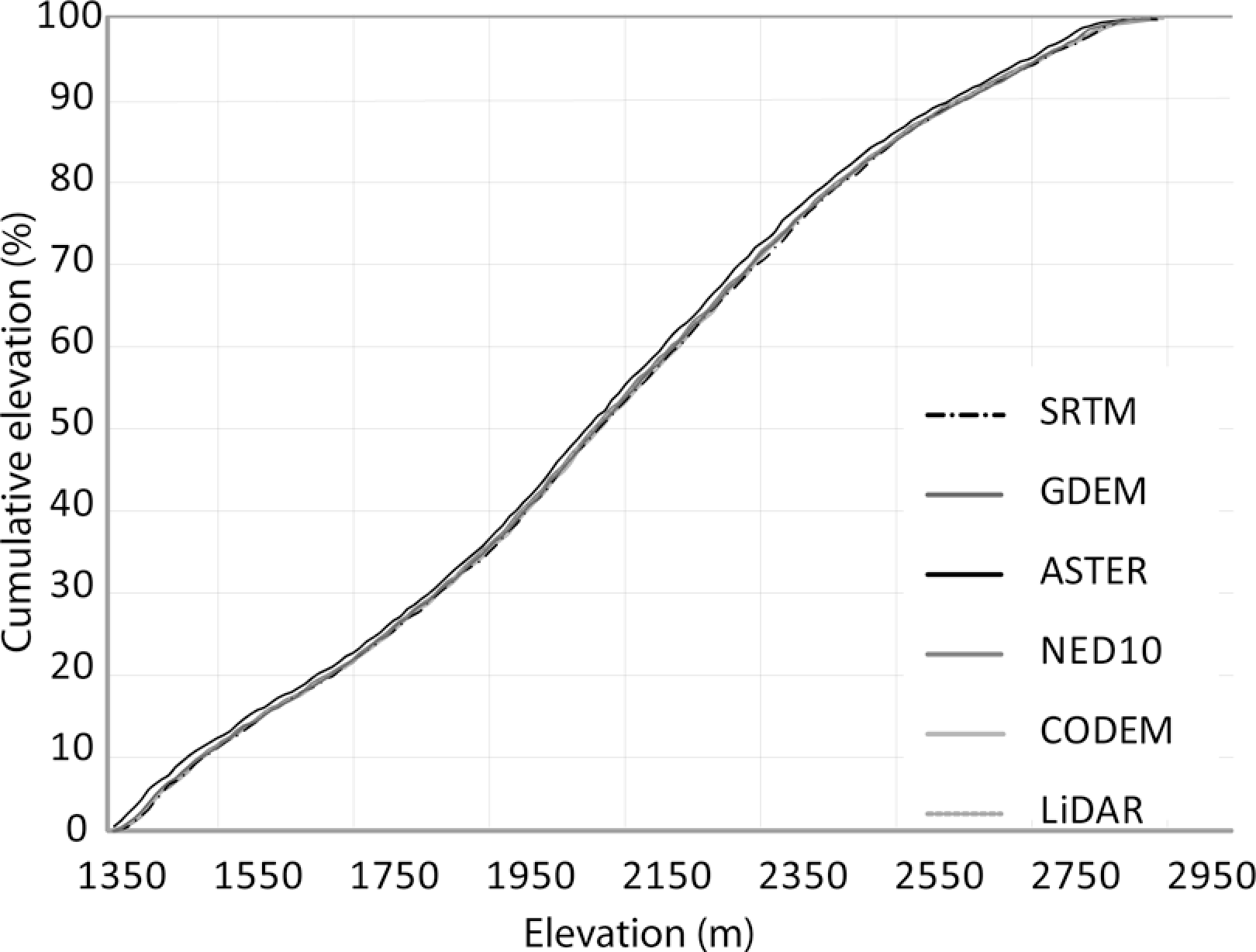
Statistical results for vertical accuracy assessment. Cumulative elevation (in %) versus elevation values for the studied DEM grids. The offset in the ASTER DEM curve reveals a shift (systematic error) requiring systematic correction to achieve realignment with the other grids (see text).
Distributions of elevation in the six DEMs. Min and Max are the minimum and maximum values; 1st and 3rd Qu. are the first and third quartile. For the ASTER DEM, corrected values (see text) are in brackets. For other DEMs, tabulated values are initial values.
RMSE results for the six DEMs. STD is the standard deviation and ME is the mean error for each DEM grid. RMSE is the initial RMSE with respect to the reference geoids used for the production of each DEM. RMSEc is the new RMSE calculated with respect to the LiDAR reference grid.
As a further test, linear regression analysis was carried out between the elevation data of each DEM and the LiDAR reference grid, respectively (Figure 5). Overall, the DEMs produced a goodness-of-fit, measured by the determination coefficient r2 , close to +1, with intervals ranging between +0.9979 for the worst fit and +0.9999 for the best. The CODEM and NED10 show the strongest correlation with the LiDAR, followed by the AstD and the GDEM. Model fits reveal outliers at different locations in the AstD, GDEM and SRTM scatter plots. The outliers reflect some of the error present within the DEM, which appears largest in the case of the AstD. However, neither data scatter in the linear regression models nor vertical accuracy constitute sufficient criteria to achieve a full definition of DEM error because the error is expressed globally (lacks any indication of spatial distribution), and because when untested spatial autocorrelation occurs in data, linear regression models tend to overestimate both strength of correlation and precision.
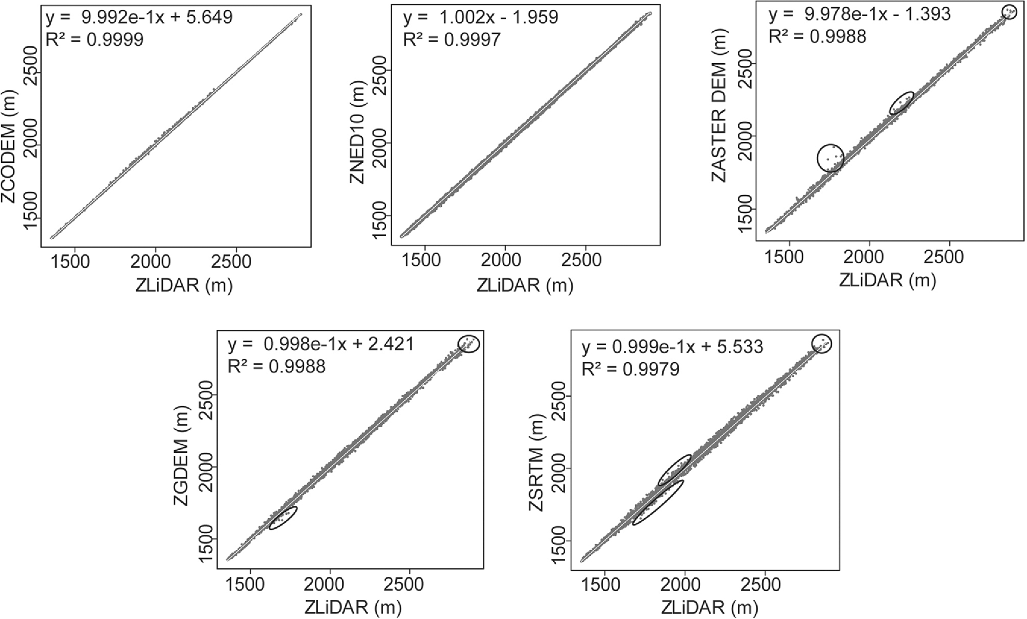
Scatter plots of elevation values (z) produced for various permutations of the studied DEM grids
2 Residual maps and computation of primary topographic attributes
One approach to locating error distribution patterns visually can be achieved through the creation of so-called deterministic error surfaces. These can be generated for a DEM by using reference data assumed to possess higher accuracy than the DEM (Hebeler and Purves, 2009), in this case the LiDAR, but equally ground control points or other surface model data (Holmes et al., 2000). In this way, maps of differences between the reference grid and other grids, termed here residual maps of either elevation or slope gradient, can provide an understanding of error sources and form a basis for further analysis (Van Niel et al., 2004). Residual maps were generated by applying an algebraic operation of pixel by pixel subtraction between each DEM and the LiDAR. In order for these tests to be meaningful, degradation of the LiDAR to the relevant ground resolutions, i.e. from 5 m to 90 m, was necessary. This operation resulted in a series of numerical images representing Re, the pixel-wise residual value (Figure 6).

Maps of Re standard deviation for elevation in the Weber Segment (colour version available online). The residual values in maps A to E express the difference between z values in each DEM and the z values provided by the LiDAR reference. (A) CODEM, cell size = 5 m. (B) NED10, cell size = 10 m. (C) ASTER DEM, cell size = 15 m. (D) GDEM, cell size = 30 m. (E) SRTM, cell size = 90 m.
Figure 6 shows that (1) the range of Re standard deviations is similar (0–11 m) for the three most accurate DEMs, namely CODEM, NED10 and AstD. (2) The SRTM and GDEM show the greatest deviations (up to 41 m) from the reference surface, which is in keeping with the lower ground resolution of these two data sets. Furthermore, the bicubic spline resampling procedure resulted in artificial smoothing of the surfaces, an aspect clearly apparent in the SRTM residual map (Figure 6E). (3) High values of standard deviation tend to cluster around the same sites in the landscape whatever the grid-cell size, with detectable variations in the sharpness of the discontinuities. (4) The highest values, i.e. greater than 9 m, follow narrow valley floors in the mountainous relief. Value distributions differ in the piedmont, where they are located along wider valleys. (5) High deviations mostly affect slopes and valley bottoms. Where hillslopes are affected by anomalous deviations, errors are likely to propagate to higher order topographic attributes (e.g. slope curvature), and hence adversely affect predictions made from the DEM for applications such as hydrology or natural hazards. (6) Flat areas, which predominate in the southern part of the piedmont zone, display values that are close to the minimal deviation, i.e. 0 m. This is most visible with the higher grid-cell sizes in Figure 6, B, C and D. Flat areas, which are often problematic in hydrological network extraction (e.g. Tarboton, 1997), thus seem to be less affected by high deviations. However, this finding does not exclude the possibility that erratic features, such as pits and holes, could be present in this kind of area. Figure 6E (SRTM) shows that regions affected by large error are larger, form continuous patches, and are concentrated in valleys and on elevated ridges whereas they are absent or more discontinuous in the other DEMs.
The following step in the procedure involved the computation of slope gradient values in order to assess error patterns in slope gradient. Slope maps depend on the choice of algorithm and on grid-cell size. We used the Zevenbergen and Thorne (1987) algorithm due to existing consensus over its relative robustness and consistent behaviour in various terrain geometries (e.g. Florinsky, 1998; Jones, 1998; Liu and Bian, 2008; Zhou and Liu, 2004b). Calculations were carried out on each of the six grids (Figure 7). Slope values range from 0° to 89.9° (Table 3). Lower values (0–1°) indicate flat interfluves or valley bottoms, whereas the highest slope angles represent unusual terrain values, typically greater than 35° and located on faceted spurs. Standard deviation and mean slope decrease with grid-cell size, in line with previous research on this topic (e.g. Kienzle, 2004; Warren et al., 2004) but unlike results obtained for DEMs extracted from contour lines (e.g. Ziadat, 2007).
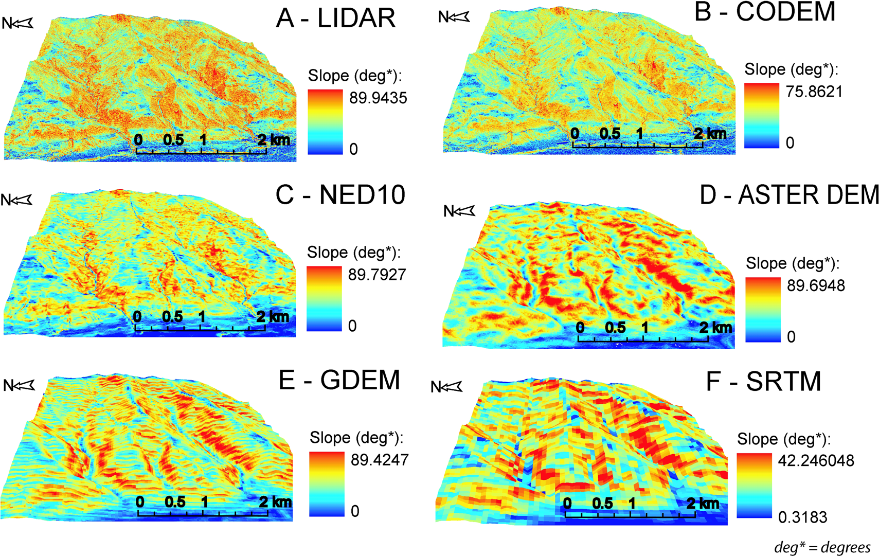
Slope maps of the Weber Segment as generated from each of the DEMs (colour version available online). (A) LiDAR, cell size = 2 m. (B) CODEM, cell size = 5 m. (C) NED10, cell size = 10 m. (D) ASTER DEM, cell size = 15 m. (E) GDEM, cell size = 30 m. (F) SRTM, cell size = 90 m.
Slope values for the six DEMs. Slope-angle range is the interval between minimum and maximum slope; mean slope angle is the arithmetic mean of the slope value distribution; Std slope is the standard deviation of that distribution.
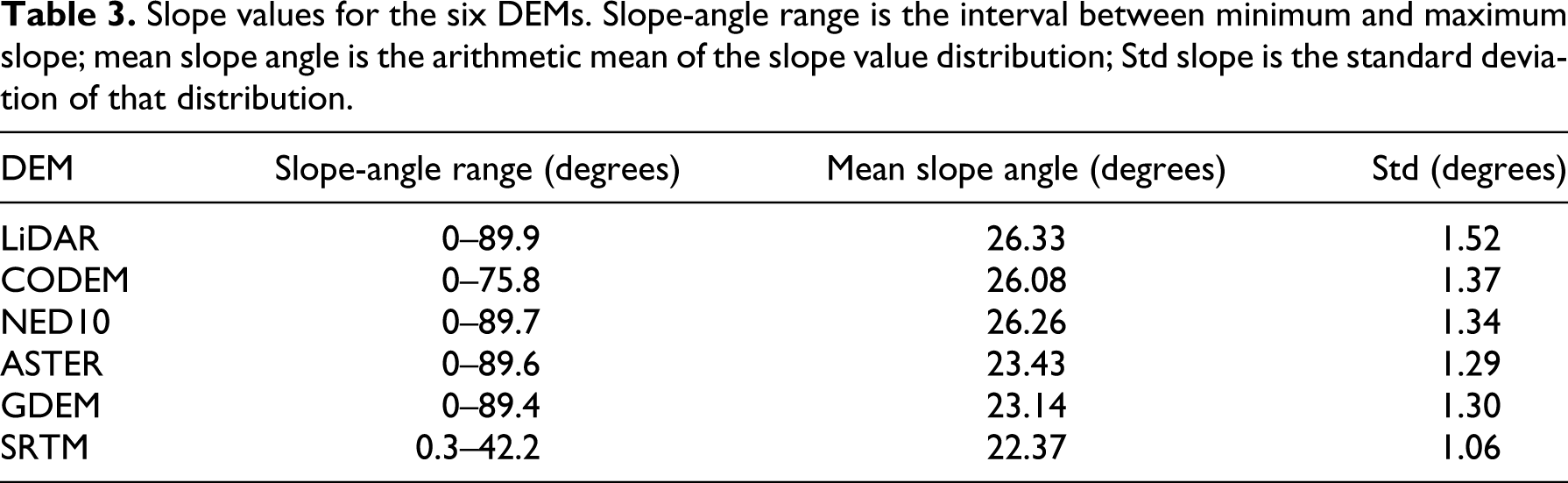
The distribution of slope values is representative of the general slope trend for all the DEMs (Figure 8). Values of 0–30° represent 98% of the slope frequency range in the SRTM, whereas other DEMs exhibit a greater proportion of extreme values (for example, slope angles greater than 40° account for 10% of the slope frequency distribution). Field data have revealed that the Weber Segment mountain front is characterized by slope angles never exceeding 43° (Eblen, 1995; Stock et al., 2009), with mean values close to 25–26°. The highest values, between 45° and 90°, are thus anomalous and represent errors due to DEM uncertainty, which were propagated to the slope map during transformation of the elevation data. The geographical location of large errors in slope coincides for each DEM with that of the largest errors in elevation (Figure 7). For angles up to 45°, slope values also increase with cell size. However, anomalous values are fewer for the larger grid-cell sizes than for the smaller ones (CODEM, NED10, AstD). This also means that the larger the grid-cell size, the greater proportion of values <45° and the fewer outliers present.

Comparative distributions of slope values for each DEM grid
Although results are so far directly ascribable to misfits originally affecting z, results differ between the mean and lower slope values. The lower 50% of the distribution frequency is marked by several offsets between the highest and smallest grid-cell sizes (Figure 8): for example, contrary to the expectation that error is consistently proportional to grid-cell size, between 0° and 25° the slope distribution values of the CODEM increase faster than for the NED10. Also, in the low range (i.e. 0° to less than 15°) the AstD curve locally crosses the SRTM and GDEM curves. Consequently, lower and mid-range slope values appear to reflect isolated discrepancies in the DEM elevation structure. The standard deviation of residuals (difference between reference and calculated slope) was also calculated (Figure 9), illustrating for each DEM the deviation in mean distribution values for each grid. In the six DEMs, the thalwegs of larger valleys are well marked. Note also that the locations of slope errors are almost identical to the locations of the errors in elevation except on the main central facets of the Weber Segment (Figure 9). The higher the terrain resolution, the more sensitive the gridded data to errors in slope, which are thus also linked to terrain roughness characteristics. Accordingly, slope deviations range between 0° and 14° for the larger grid-cell sizes (SRTM, GDEM) and between 0° and 25° for the smaller (LiDAR, CODEM, NED10, AstD; Figure 9).

Maps of Re standard deviation for slope angle in the Weber Segment (colour version available online). Key as in Figure 6.
The strength of the relationship between errors in slope and errors in elevation (Figures 6 and 9) was tested by performing a linear regression between elevation (Re on elevation) and slope residuals (Re on slope). A non-linear relationship between those two variables was found (Figure 10). However, the form and intensity of the relationship is biased by several outliers that stretch the scatter plot in several directions. Determination coefficients with values <0.3 for the SRTM and CODEM and <0.1 for the AstD, GDEM and NED10, indicate weak to no dependency between the errors in slope and in elevation. In other words, only 10–30% of anomalous slope values (in particular among the lower and mid-range values) can be explained by anomalous elevation values. Such a conclusion, however, is potentially spurious because r2 is not a robust criterion for explaining either the numerical or the spatial behaviour of errors affecting slope. Accordingly, as a further tool for evaluating whether higher error affecting elevation was positively correlated with higher error affecting slope, we inspected the data grids for spatial autocorrelation.

Scatter plots highlighting links between errors in elevation and in slope for various permutations of the studied DEM grids
3 Spatial autocorrelation analysis
Calculation and 2.5-D mapping of Moran’s I and LISA were used to identify areas with a high risk of error caused by pixels being surrounded by similar areas or by spatial outliers, and as tools for visualizing the location of uncertainty. A spatial weighting matrix was used for each variable, and was defined at varying distance lags corresponding to the respective DEM resolutions. The weighting process was carried out using Rook’s case–contiguity kernel, with symmetrical spatial weights wij = 1 when locations i and j are adjacent, and wij = 0 in other cases. Rook’s case considers the neighbourhood of four locations adjacent to each cell (Elobaid et al., 2009). A Monte Carlo randomization procedure allowed us to assess significance levels by performing 999 permutations (i.e. tests) for each grid (Table 4).
Autocorrelation results for errors on elevation and on slope. Moran’s I elevation and Moran’s I slope are the univariate Moran’s I calculations for the dependent (elevation) and independent (slope) variables, respectively. Bivariate Moran’s I refers to the errors in elevation and in slope and is the result of the multivariate LISA test.
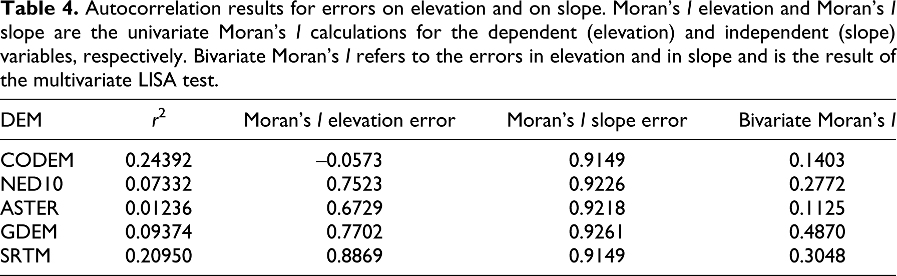
The randomization test avoids relying on assumptions about data distribution and developing statistical moments under a null hypothesis, and avoids testing all types of statistic analytically (Aubry and Piégay, 2001). Significance levels are given by the p-values (arbitrary threshold), are calculated for each cluster, and allow significant autocorrelation values to be identified. After trial comparisons with other thresholds (0.0001, 0.001, and 0.01) for each DEM, p-value significance levels were set to 0.05 because this configuration yielded the highest and most sharply differentiated levels of data clustering. Table 4 summarizes global clustering levels for bivariate and univariate variables, each time for a run of 999 permutations.
The CODEM grid, with a Moran’s univariate I of about –0.06, illustrates a situation of low negative spatial autocorrelation, implying that neighbours are dissimilar and that error values affecting elevation do not have a unique source or cause. In contrast, error values in the other DEMs obtain a Moran’s index close to +0.9, indicating a strong spatial link between errors in elevation. Error in slope systematically attains values close to +1, with a high level of spatial dependence showing strong positive spatial autocorrelation values. Where high spatial autocorrelation scores were observed for elevation, values likewise increased for slope, thus confirming a mechanism that drives the disproportionate (i.e. non-linear) propagation of errors in elevation to errors in slope gradient. The bivariate Moran’s index, which describes the magnitude and relationship of global error between elevation and slope, is characterized by positive values but none of these are close to +1. The strongest positive relations are observed for the GDEM (+0.4870) and SRTM (+0.3048) grids, whereas the lowest occur in the AstD (+0.1125). Results are thus similar to the univariate values except for the AstD. The SRTM, GDEM and NED10 present a high level of clustering, with the CODEM ranking last.
The LISA helps to bring out local magnitudes of error clustering. Each observation provides a measure of the extent of statistically significant spatial clustering of similar error values around a data point. LISA results reveal a high level of differentiation within each DEM (Figure 11). High–high and low–low clusters define a high error value surrounded by high values and a low value surrounded by low values, respectively. Such situations are present in the SRTM, GDEM and to a lesser extent the NED10 grids. A higher risk of error propagation occurs where high–high values are found. Relative stability, i.e. a low risk of error propagation to higher order topographic derivatives, prevails in low–low situations. High–high clusters are found in the same locations as in the univariate elevation and slope error maps. In those cases, therefore, the LISA maps merely corroborate previous results. Uncertainty in slope is thus highly correlated with initial elevation, and thus with error in elevation, which in turn conditions the spatial distribution of errors.

Uncertainty cluster maps based on the LISA (colour version available online)
For grids other than the SRTM, GDEM and NED10, LISA maps show somewhat different results. AstD maps show all the peak occurrences already found in the SRTM and GDEM grids, but low–high and high–low clusters are more prominent between high–high clusters. High–high levels are typical of major thalwegs and low-lying areas. In the case of the NED10, error distribution patterns bring out geomorphological features (particularly ridges and escarpments) more sharply than the SRTM and the GDEM. This arises whatever the level of p-value significance (tested from 0.0001 to 0.05). The CODEM stands as the exception: uncertainty already detected in previous maps (Figures 7 and 9) is well represented in the CODEM LISA map but fails to show the high or low clustering levels encountered in the other DEM grids. Clustering is less intense (note the predominance of half-tones), illustrating uncertainty in the data, i.e. uncertainty not linked to terrain characteristics and presumably caused by other unknown factors which would remain to be investigated.
V Summary and conclusion
The aims of this article were: (1) to review suitable tools for assessing error in remotely sensed data and for calibrating DEM studies that focus on primary topographic attributes; (2) to investigate a statistical tool more often used in ecology and human geography than in digital terrain analysis, namely LISA clustering, which helps to produce and evaluate error maps in order to track DEM error propagation; and (3) to assist in decision-making when selecting among a range of DEM products that are readily available for a chosen study area. In a worked example involving terrain analysis in the Wasatch Mountains of Utah, we were able to use LiDAR data as a surrogate for field control points. We tested five other, freely available, DEM grids against this very high-resolution reference grid.
Despite the existing catalogue of methods for removing various categories of error in gridded data, the overriding conclusion at present is that errors can never be totally erased from DEMs. Empirical approaches work best when higher-quality reference data are available for comparison and allow a range of statistical ranking procedures to be carried out. Initially, basic quantitative tools such as the RMSEc were of little use in determining DEM accuracy. It was shown that the larger the grid-cell size, the lower the accuracy, with nevertheless a fair degree of reliability in z whatever the sensor type and whatever the original data ingredients entered into the DEM. The CODEM, NED10, AstD, GDEM and SRTM could therefore be used almost indiscriminately for basic displays of topography, depending simply on choice of resolution for graphic output.
As an improvement on RMSE procedures we generated a series of residual elevation and residual slope maps (Re), which provided an outline of the spatial distribution of errors based on calculations of the standard deviation of Re. Two main conclusions arose from these findings: (1) errors in slope and in elevation are linked, but with a variable strength of dependency as shown by linear regression results; and (2) the SRTM, GDEM and NED10 stand out for their lower error scores. Irrespective of their ground resolutions, the CODEM and the AstD presented either more extreme error values or more confused results. This finding argues against preferring these data sources for morphometric or hydrological applications. Re results emulated a further approach in error analysis using Moran’s I and LISA maps. This approach has revealed that the intensity of spatial autocorrelation is not linked to grid-cell size. It is more closely related to the intrinsic characteristics of DEM products and to procedures dealing with slope gradient calculation. The LISA maps also help to define error hot- and coldspots, i.e. high–high and low–low clusters. Among the five DEMs analysed in this study, the autocorrelation tests finally allowed the NED10 to stand out as the DEM least affected by the presence of error and its propagation. Like the CODEM, the NED10 is a hybrid DEM compiled from a range of digital and non-digital sources rather than from unique radar or optical sources, and also happens to be of a lower native resolution.
The trends and topics reviewed here have emphasized the value of exploring gridded data structures for detecting spatial error patterns because results can be used for ranking DEM quality. Such procedures seem critical for most practical terrain applications in natural catchments, but also for using the DEM grids as input substitutes for ‘real topography’, i.e. as initial conditions for running predictive surface process models (e.g. Codilean et al., 2006) and observing how the landscape evolves under given conditions (heuristic terrain modelling). Despite its advantages, the LISA still remains a semi-quantitative tool (values express variations in clustering as ‘high’ or ‘low’). A move towards more fully quantitative characterizations of error in DEMs, where, in addition to its location, the intensity of error is provided (deviation of elevation in metres, and/or slope in degrees), could perhaps be achieved by coupling the LISA with other error modelling methods such as geostatistical simulations based on kriging, or geographically weighted regression (Fotheringham et al., 2002).
Footnotes
Acknowledgements
We are grateful to Editor-in-Chief Nicholas Clifford for steering our manuscript through a high-quality reviewing process, with fine reports from several anonymous referees who greatly improved the scope and structure of this contribution.
Appendix
(a) Artifacts, blunders and gross errors
Reuter et al. (2009) defined artifacts as erratic features that appear on a DEM as holes, ghost lines, stripes and so on. Artifacts and associated errors could even have been invisible in the input DEM but can be inferred from unrealistic values occurring on elevation derivative maps. Blunders are vertical errors associated with data collection. They can be mistakes caused by misreading contours, by transposing numerical values, by erroneous correlations, or by careless observations (Wechsler, 2003). Gross errors occur when a measurement process is subject to occasionally large inaccuracies and generates data outliers. It includes topographical misinterpretations, and long linear features along some boundaries of the calculation window used in DEM interpolation (Oksanen, 2003). Some techniques such as ‘data snooping’ are efficient at detecting them (Karras and Petsa, 1993), and inspection of a shaded relief map can also help (Gousie, 2005).
(b) Systematic errors
Sytematic errors result from deficiencies in measurement or processing and affect the accuracy of the final data, i.e. the degree to which the final data agree with reality. Systematic errors are also identified as residual systematic error surfaces caused by slightly inaccurately estimated lens distortion parameters (Wise, 2000), by translation effects, or false features such as phantom tops, ridges, benches or striations (Raaflaub and Collins, 2006). In general, they reflect bias inherent in the data collection method (Reuter et al., 2009).
(c) Random errors
Random errors result from mistakes such as inaccurate surveying or improper recording of elevation information. Often associated with signal noise, random errors are extracted after known blunders and systematic errors have been removed (Podobnikar, 2009; Reuter et al., 2009; Wechsler, 1999, 2006; Zhang and Cen, 2008).
(d) Uncertainty
Uncertainty is a term employed when a modelled value deviates from its true value, with a confidence interval (Hebeler and Purves, 2009). Lack of knowledge about measurement reliability and about its representation of true values is referred to as its uncertainty and is a measure of what we do not know (Wechsler, 1999, 2006). DEM uncertainty thus covers lack of knowledge about parameters, model assumptions, and scenarios, i.e. spatial evolution models (Liu and Bian, 2008).
(2)
(a) Root mean square error and mean error
(b) Bicubic spline formula
(c) Residual maps and standard deviation algorithms Pixel by pixel algebraic subtraction of elevation values provides a series of residual values (Re) that can be mapped: