Information retrieval in physical geography

Abstract

Information retrieval (IR) methods seek to locate meaningful documents in large collections of textual and other data. Few studies apply these techniques to discover descriptions in historical documents for physical geography applications. This absence is noteworthy given the use of qualitative historical descriptions in physical geography and the amount of historical documentation online. This study, therefore, introduces an IR approach for finding meaningful and geographically resolved historical descriptions in large digital collections of historical documents. Presenting a biogeography application, it develops a ‘search engine’ using a boosted regression trees (BRT) model to assist in finding forest compositional descriptions (FCDs) based on textual features in a collection of county histories. The study then investigates whether FCDs corroborate existing estimates of relative abundances and spatial distributions of tree taxa from presettlement land survey records (PLSRs) and existing range maps. The BRT model is trained using portions of text from 458 US county histories. Evaluating the model’s performance upon a spatially independent test dataset, the model helps discover 97.5% of FCDs while reducing the amount of text to search through to 0.3% of total. The prevalence rank of taxa in FCDs (i.e. the number of times a taxon is mentioned at least once in an FCD, divided by the total number of FCDs, then ranked) is strongly related to the abundance rank in PLSRs. Patterns in species mentions from FCDs generally match relative abundance patterns from PLSRs. However, analyses suggest that FCDs contain biases towards large and economically valuable tree taxa and against smaller taxa. In the end, the study demonstrates the potential of IR approaches for developing novel datasets over large geographic areas, corroborating existing historical datasets, and providing spatial coverage of historic phenomena.

Keywords

Biogeography boosted regression trees forest composition historical documents historical ecology information retrieval machine learning presettlement land survey records text mining

I. Introduction

Approaches in information retrieval (IR) have sought to extract meaningful documents from large collections, including by ranking documents based upon relevance to a set of search terms (e.g. Tyree et al., 2011). Related methods in text mining (TM) have sought to derive information from large datasets of unstructured text, such as through the classification and clustering of text documents (Feldman and Sanger, 2007). IR and TM applications are diverse and have extended into physical geography realms, such as to assess scholarly literature coverage of marine species (Fisher et al., 2011), to discover trophic links based on co-occurrences of species in scholarly literature (Tamaddoni-Nezhad et al., 2013), and to reconcile land cover type classifications among varying classification systems (Comber et al., 2015; Wadsworth et al., 2009).

One research area with potential for IR and TM applications is the study of historical natural conditions and natural events in physical geography. Researchers have long consulted various historical documents that include local histories, early scientific literature, traveler accounts, and legal documents (Hooke and Kain, 1982; Ruffner, 2006; Whitney, 1996). Historical documents have provided glimpses into diverse topics such as past forest structure and composition (Whitney, 1996), Native American fire use (e.g. Stewart, 2002), and historical tropical cyclone frequencies (e.g. Chenoweth, 2006). Elsewhere, historical documents have been used to support quantitative methods; for example, Black et al. (2006) and Tulowiecki (2015) cited 17th–18th-century CE documents to support findings regarding past forest composition produced using statistical methods. Pederson et al. (2014) consulted historical documents, such as diaries and newspapers, to explain disturbance events (e.g. droughts) inferred to have been recorded in tree-ring records dating back to the 18th century in the eastern US. As reviewed by Grabowski and Gurnell (2016), documentary sources have also been used to reconstruct historical conditions and events in fluvial geomorphology. Collectively, these works often face limitations in that (1) few documents are searched relative to the potential amount of freely available digitized documents, (2) using historical documents is sometimes relegated to location-specific (Edmonds, 2005) applications in support of results produced by other data and methodologies, or (3) more rigorous methods of searching for qualitative information from documents are not explored.

One potential means for automating the search for meaningful historical data from digitized documents is through IR methods, namely by ranking documents or portions of text based upon their relevance to a topic. IR methods, such as Internet search engines, generally work in two steps. First, due to the large volume of documents to search through, a subset of indexed documents that are related to a user’s search terms (e.g. documents containing the search terms) are selected using faster, more approximate IR approaches (e.g. Broder et al., 2003). Second, a predictive model trained a priori ranks the subset of documents based upon their potential relevance to the same search terms given by the user. This predictive model in itself is trained with a binary dependent variable (i.e. ‘relevant’ or ‘not relevant’), and predictor variables comprising a set of text ‘features’, such as the presence/absence or frequencies of the search terms in the documents (Weiss et al., 2015). These models are trained through various means, including through human ‘labeling’ of pages by relevance to the search terms, or through automated means such as ‘clickthrough logs’ maintained by search engine companies (e.g. Joachims, 2002). It is noteworthy that many modeling techniques used in IR machine-learning approaches are also those sometimes applied in physical geography studies; for example, boosted regression trees (BRT), neural networks, random forests, and support vector machines are techniques applied in both IR web-search ranking (Tyree et al., 2011) and in species distribution modeling (Franklin and Miller, 2009).

The purpose of this study is to present and test the efficacy of an IR method for finding geographically resolved historical descriptions for physical geography applications, within large volumes of digitized historical documents. The utility of this method is explored through a biogeographical application, specifically by developing a predictive model or customized ‘search engine’ to identify descriptions of historical forest composition within digitized county histories of the US (circa 18th–19th centuries). A model developed using machine-learning methods will be created to rank portions of text by their probability of containing a relevant forest description, based upon counts of key terms. This study then examines the value of the method by testing the usefulness of descriptions of forest composition, through comparisons of the descriptions with estimates of taxa relative abundances and geographical distributions made from other historical datasets, including presettlement land survey records (PLSRs). In this manner, this study explores the potential value of the IR method for corroborating existing historical datasets in novel ways, for compiling novel historical datasets over large geographic areas, and for providing spatial coverage of historic phenomena where other historical records are not present.

This study’s application is to find forest compositional descriptions (FCDs) in county histories, defined here as historical forest descriptions that describe tree taxa at a location. A preliminary review of county histories of the US and other literature on pre-Euro-American landscapes (Whitney, 1996) revealed that FCDs were common in historical documents, summarizing forest composition for a geographic area (e.g. Figure 1). Such FCDs described forests growing in different locations, topography, or soil conditions within a geographic area. Some FCDs summarized forest composition at the time of Euro-American arrival, whereas other descriptions summarized composition at the time of the text’s publication (often 19th century in this study). This study’s foci were FCDs that were predominately ecological in purpose, rather than descriptions inferred to have overtly utilitarian, poetic, or other purposes (Whitney, 1996). While writers described forests at other resolutions (e.g. county), early investigations revealed that most FCDs occurred at the town or township resolution, making these FCDs the focus of the study. In this study, ‘township’ is used to describe entities in Ohio, whereas ‘town’ is used for entities elsewhere or to describe all similarly sized geographic entities collectively throughout the areas studied.

Figure 1.

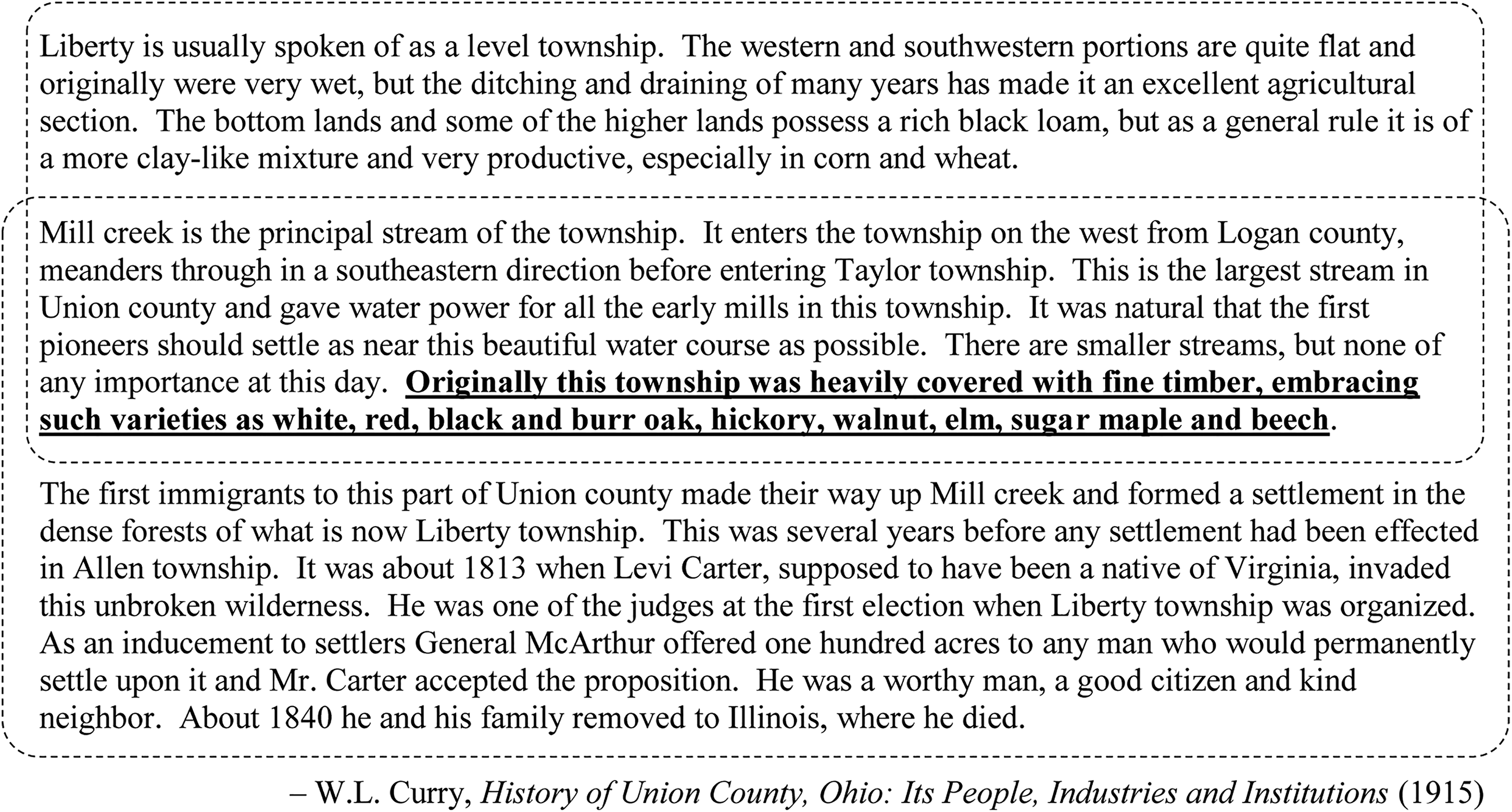
An example of a forest compositional description (FCD) for Liberty Township, Union County, Ohio, USA (Curry, 1915). The FCD includes tree taxa comprising six genera: oak (Quercus spp.), hickory (Carya spp.), walnut (Juglans spp.), elm (Ulmus spp.), maple (Acer spp.), and beech (Fagus grandifolia).

II. Materials and methods

Section II.1 describes the development of a predictive model to rank portions of text within county histories by their probability of containing FCDs. Section II.2 describes the analyses performed to examine the applicability of FCDs and the IR method.

1. Developing a predictive model

A model was developed to generate a probability that a FCD was present in a portion of text based upon the counts of key terms, to be used for ranking text for additional examination. Each of the four steps used to develop the model is described below.

1.1 Acquiring county histories

This study acquired digitized versions of county histories of the eastern US, which were used to execute this study’s purpose for two reasons. First, county histories are spatially extensive: approximately 80% of US counties possess at least one county history (Meyerink, 1998). Second, digitized county histories are widely accessible from online repositories such as Internet Archive (2017), HathiTrust Digital Library (HathiTrust, 2017), and Google Books (Google, 2017); subscription-based online databases (e.g. ProQuest’s HeritageQuest Online, 2015); and statewide collections (e.g. University at Michigan’s Michigan County Histories and Atlases Digitization Project, 2007). County histories were downloaded from the Internet Archive (2017) in a plain text format that was converted from scanned formats via optical character recognition (OCR) technology. Histories were generally located using county and state names as search terms. Only public-domain county histories (i.e. published prior to 1923) were downloaded.

One set of county histories (n = 458) from 13 states (Figure 2) provided a set from which to select samples for the model’s training dataset (Section II.1.3). Of 568 county histories for this geographic area that were both listed in a county history bibliography by Filby (1985) and published prior to 1923, 319 (56.2%) were represented in part or whole by the volumes obtained for this study; 74 volumes obtained were not listed in Filby (1985). Ninety percent of histories obtained were published between 1851 and 1920. Another set of county histories from Ohio (n = 174; Figure 2) provided a spatially independent test dataset upon which to assess performance of the model. Of these 174 volumes, 40 were uploaded from Google Books to Internet Archive by the author of this study. Of the 194 county histories for Ohio that were both listed in Filby (1985) and in the public domain, 149 (76.8%) were represented in part or whole by the volumes obtained; 10 volumes obtained were not listed in Filby (1985). Ninety percent of histories obtained for Ohio were published between 1871 and 1920.

Figure 2.

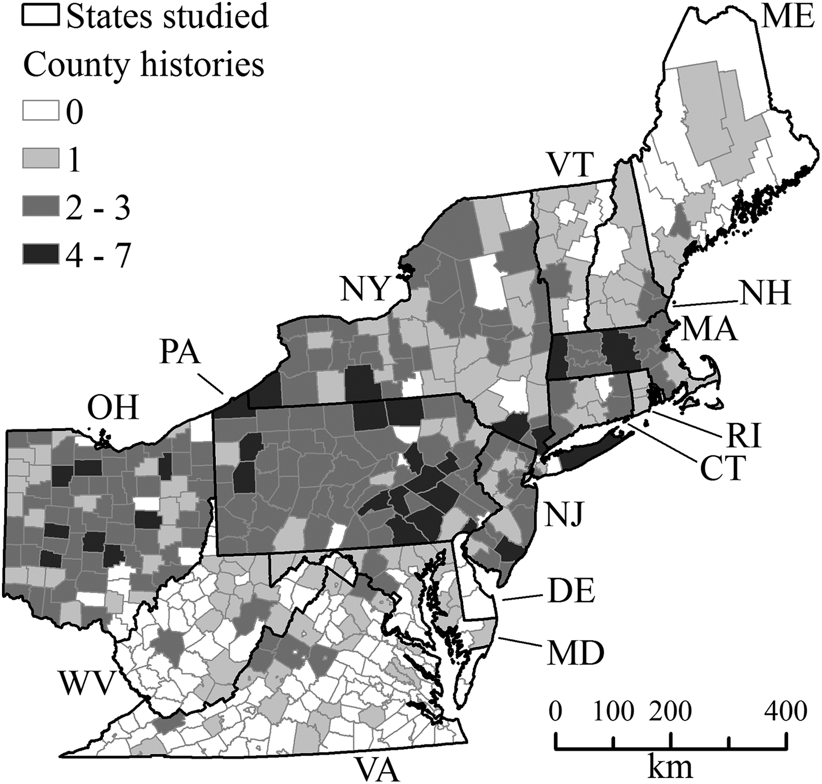
A map showing the study area, and indicating the number of county histories acquired for the training (i.e. the 13 easternmost US states) and test (i.e. state of Ohio) datasets per county, mapped using modern county borders. Multiple volumes of the same county history were treated as a single text in this map. The states are: Connecticut (CT), Delaware (DE), Maine (ME), Maryland (MD), Massachusetts (MA), New Hampshire (NH), New Jersey (NJ), New York (NY), Ohio (OH), Pennsylvania (PA), Rhode Island (RI), Vermont (VT), Virginia (VA), and West Virginia (WV).

1.2. Creating predictor and dependent variables

A Python script (see online supplementary material) was written and implemented in PythonWin (Hammond, 2008), which first divided each county history into two-paragraph overlapping ‘text chunks’, and then counted the number of key terms in each text chunk related to FCDs to form predictor variables. Text chunks were overlapping, in that each paragraph was present in two text chunks (Figure 1); later steps ensured independence of samples for model training and testing. After testing preliminary models developed from training datasets with only one paragraph per sample, documents were split in this manner to ensure an adequate length of text for counting the number of key terms.

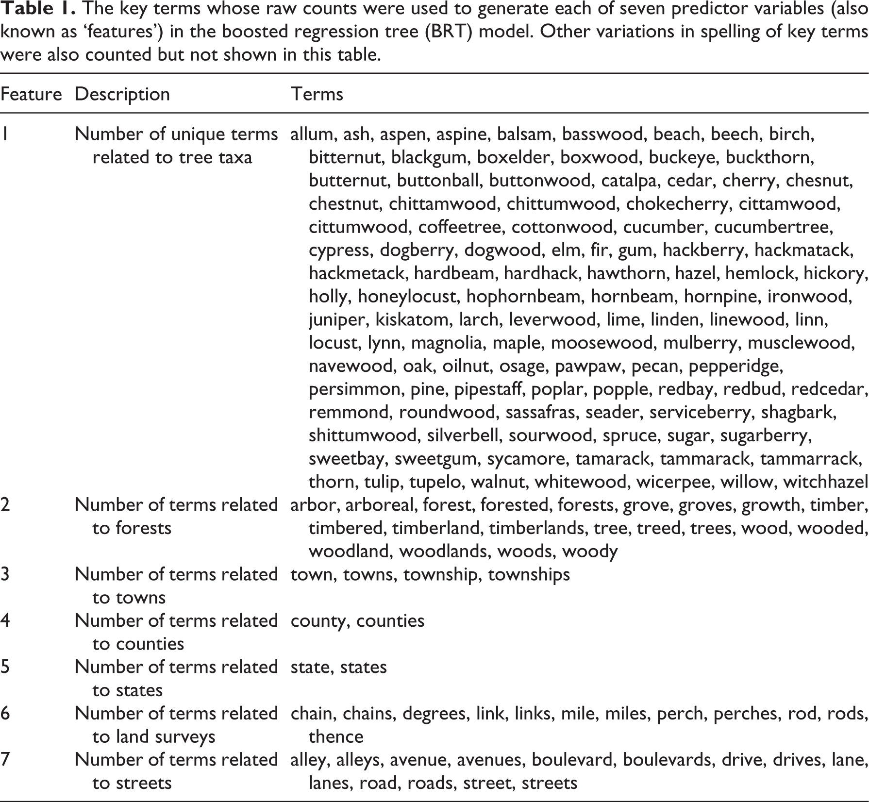
Seven features of text chunks believed to be positively or negatively correlated with FCDs were chosen as predictor variables (Table 1). Whereas Features 1 through 3 were believed to be positively correlated with the probability of the text chunk containing a town-resolution FCD, Features 4 through 7 were believed to be negatively correlated. The list of terms comprising Feature 1 was aided by two lists of common names for trees in the eastern US: the Climate Change Tree Atlas (US Department of Agriculture, 2017) and Cogbill et al. (2002). Features 4 and 5 were included to attempt to separate out FCDs reported at county or state extents. Feature 6 was included to distinguish text chunks containing descriptions of early land surveys (e.g. ‘beginning at an oak post, thence north’) that occasionally appeared in county histories. Feature 7 was included to separate out text chunks containing descriptions of street names (e.g. ‘Oak Street’). The Python script performed steps to increase the accuracy of counting the number of key terms, such as by removing problematic extraneous characters, performing lemmatization (also known as ‘stemming’) on key terms, and accepting plural forms and slight variations in spelling (e.g. ‘cottonwood’, ‘cottonwoods’, ‘cotton wood’, and ‘cotton woods’, all counted as ‘cottonwood’). The terms ‘features’ and ‘predictors’ are used somewhat interchangeably in this study, as the former is used by those familiar to IR or TM, whereas the latter is used by those familiar with statistical modeling.

Table 1.

The key terms whose raw counts were used to generate each of seven predictor variables (also known as ‘features’) in the boosted regression tree (BRT) model. Other variations in spelling of key terms were also counted but not shown in this table.

Feature	Description	Terms
1	Number of unique terms related to tree taxa	allum, ash, aspen, aspine, balsam, basswood, beach, beech, birch, bitternut, blackgum, boxelder, boxwood, buckeye, buckthorn, butternut, buttonball, buttonwood, catalpa, cedar, cherry, chesnut, chestnut, chittamwood, chittumwood, chokecherry, cittamwood, cittumwood, coffeetree, cottonwood, cucumber, cucumbertree, cypress, dogberry, dogwood, elm, fir, gum, hackberry, hackmatack, hackmetack, hardbeam, hardhack, hawthorn, hazel, hemlock, hickory, holly, honeylocust, hophornbeam, hornbeam, hornpine, ironwood, juniper, kiskatom, larch, leverwood, lime, linden, linewood, linn, locust, lynn, magnolia, maple, moosewood, mulberry, musclewood, navewood, oak, oilnut, osage, pawpaw, pecan, pepperidge, persimmon, pine, pipestaff, poplar, popple, redbay, redbud, redcedar, remmond, roundwood, sassafras, seader, serviceberry, shagbark, shittumwood, silverbell, sourwood, spruce, sugar, sugarberry, sweetbay, sweetgum, sycamore, tamarack, tammarack, tammarrack, thorn, tulip, tupelo, walnut, whitewood, wicerpee, willow, witchhazel
2	Number of terms related to forests	arbor, arboreal, forest, forested, forests, grove, groves, growth, timber, timbered, timberland, timberlands, tree, treed, trees, wood, wooded, woodland, woodlands, woods, woody
3	Number of terms related to towns	town, towns, township, townships
4	Number of terms related to counties	county, counties
5	Number of terms related to states	state, states
6	Number of terms related to land surveys	chain, chains, degrees, link, links, mile, miles, perch, perches, rod, rods, thence
7	Number of terms related to streets	alley, alleys, avenue, avenues, boulevard, boulevards, drive, drives, lane, lanes, road, roads, street, streets

The number of key terms (Table 1) were counted for the text chunks comprising the final training and test datasets (described in Sections II.1.3 and II.1.4). Training and test datasets were then hand-labeled with a ‘1’ (part or all of a FCD is present) or ‘0’ (no portion of a FCD is present) to form the dependent variable.

1.3. Training the model

Samples for model training (n = 1818) were selected from text chunks with one (e.g. ‘…oak…’) or more unique mentions of a tree taxon from the training dataset. To ensure a representative sample of text chunks with varying combinations of key term counts comprising each feature (Table 1), text chunks were classified into 40 clusters based on feature counts, using k-means clustering and a scree plot implemented in ‘R’ (R Development Core Team, 2011). A random sample of 50 text chunks maximum in each of the 40 clusters made up the training dataset. Only three clusters had less than 50 text chunks, and any text chunk that shared a paragraph with another text chunk (e.g. Figure 1) was eliminated to preserve independence of samples.

A BRT model was trained to predict the probability of a FCD occurring within a text chunk. This machine-learning technique was chosen since it is used in other IR applications, including web-search ranking; in a ranking competition organized by Yahoo Labs, BRT was used by all top eight teams (Tyree et al., 2011). BRT is also a technique widely applied for species distribution modeling (Elith et al., 2008; Franklin and Miller, 2009), and, therefore, may be familiar to and adaptable by biogeographers. The BRT model was developed and implemented using the ‘dismo’ (Hijmans et al., 2013) and ‘gbm’ (Ridgeway, 2013) packages within R (R Development Core Team, 2011), using counts of key terms (Table 1) as predictor variables, and the binary values indicating the presence/absence of FCDs as the dependent variable.

BRT is a machine-learning technique that generates a predicted probability using a series of regression trees (Elith et al., 2008; Friedman, 2001, 2002). Using BRT, a regression tree is first trained upon a random subset of data. Splits in the regression tree are made to minimize predictive deviance in the subsets of data, until the maximum allowable number of splits (the ‘tree complexity’, or tc, reflecting the number of allowable variable interactions) is reached. The next tree is developed using the residuals that result when the prior regression trees are applied to predict upon a new random subset of data. The ‘learning rate’, or lr, determines the contribution of each tree to the final BRT model. Using the gbm.step cross-validation method for model optimization in the dismo package (Hijmans et al., 2013), a lr was selected that achieved between 1000 and 2000 regression trees (Elith et al., 2008). The tc was set to seven to allow for seven-way interactions among all predictor variables.

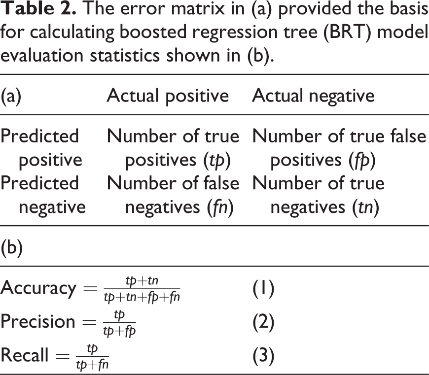
After model training, two thresholds in predicted probabilities were calibrated for classifying text chunks in the training dataset as containing or not containing an FCD, prior to applying the model to rank and classify text chunks in the test dataset. Threshold 1 was selected to maximize the sum of the true positive rate and true negative rate in the training dataset (Table 2). Threshold 2 was selected such that all of the text chunks in the training dataset identified as containing an FCD were classified as such by the model (i.e. recall = 100%). Threshold 2 was used to understand how much text would need to be classified as containing an FCD by the model for further human examination in order to discover virtually all of the actual FCDs.

Table 2.

The error matrix in (a) provided the basis for calculating boosted regression tree (BRT) model evaluation statistics shown in (b).

(a)	Actual positive	Actual negative
Predicted positive	Number of true positives (tp)	Number of true false positives (fp)
Predicted negative	Number of false negatives (fn)	Number of true negatives (tn)
(b)
Accuracy = $\frac{t p + t n}{t p + t n + f p + f n}$		(1)
Precision = $\frac{t p}{t p + f p}$		(2)
Recall = $\frac{t p}{t p + f n}$		(3)

1.4 Testing the model

The BRT model was applied to predict the presence of FCDs within text chunks of the test dataset (i.e. Ohio county histories) with two (e.g. ‘…oak, hickory…’) or more unique mentions of tree taxa. Text chunks containing only one unique mention of a tree taxon were omitted from model testing, since those text chunks dramatically increased the number of text chunks required for hand-labeling, and since the high number of non-FCD text chunks with one unique taxon mentioned would inflate the predictive accuracy of models as judged by evaluation statistics (next paragraph). This step was also somewhat analogous to IR approaches that first reduce the extremely large number of documents to a subset that are then ranked by relevance (Section I). All text chunks with two or more unique mentions of tree taxa were hand-labeled as containing or not containing an FCD prior to model testing.

The model’s predictive performance was evaluated using one threshold-independent and three threshold-dependent evaluation statistics (Table 2). The statistics were as follows. (1) The area under the receiver operating characteristic curve (AUC) produces a score that ranges from 0 to 1, equaling the probability that the model will assign a higher probability value to a random actual presence (i.e. a text chunk with a FCD) than a random actual absence (Fawcett, 2006). (2) Accuracy (Table 2: equation (1)) is the percentage of text chunks correctly classified overall (either as having or not having a FCD). (3) Precision (Table 2: equation (2)) is the percentage of text chunks predicted as containing a FCD that actually contained a FCD. (4) Recall (also known as ‘true positive rate’; Table 2: equation (3)) is the percentage of actual text chunks with a FCD that were correctly predicted as having a FCD. Threshold-dependent statistics were calculated using each threshold chosen using the training dataset (Section II.1.3). Because text chunks were overlapping, the threshold-dependent evaluation statistics were also calculated on two different test datasets from the Ohio county histories to offer different assessments of model performance: (1) a dataset of all text chunks (non-independent samples), and (2) a dataset of only text chunks with the highest predicted probability from each pair of overlapping text chunks (independent samples; Figure 1).

Model performance was evaluated in three other ways. First, characteristics of text chunks containing FCDs that were not correctly classified by the model were examined to assess potential causes for their incorrect classification. Second, precision and recall were calculated for text chunks grouped by unique number of mentions of tree taxa, to gain an understanding of the BRT model’s ability to predict the presence of FCDs across varying amounts of biogeographical data. Third, the total reduction in text to search through from the county histories, when text chunks were classified as containing an FCD, was quantified.

Characteristics of the BRT model predictor variables (also known as ‘features’) were examined in three ways. First, predictor variable importance was calculated as the sum of the number of times a variable is selected for splitting in the regression trees, weighted by the squared improvement to the model brought by those splits, and scaled to represent a variable’s percent importance (Elith et al., 2008). Second, to examine and describe the relationships between dependent and predictor variables, partial dependence plots were created for each predictor. Third, a three-dimensional partial dependence plot was created for the most important two-way variable interaction, using the methods of Elith et al. (2008). This plot was generated by varying only the values of the two predictors comprising the most important two-way interaction while holding all other predictor values at their mean value, in order to graph in three dimensions the relationships with the predicted probability.

2. Investigating FCDs

Analyses were performed to offer insight into the characteristics and usefulness of FCDs discovered by the BRT model. Analyses described basic spatial and biogeographical characteristics of FCDs (Section II.2.1) and explored the data quality of FCDs by assessing their similarity to quantitative data on tree taxon composition and distribution prior to Euro-American settlement (Section II.2.2). All mapping and geographic information systems (GIS) tasks described in the following were performed using Esri’s ArcMap 10.5^{.1 (2017)}.

2.1. Describing basic characteristics of FCDs

FCDs from the test dataset (i.e. Ohio county histories; Section II.1.1) were mapped, and the characteristics of FCDs were recorded. The Ohio histories were used because these histories were more thoroughly examined while evaluating the effectiveness of the BRT model (Section II.1.4), and, therefore, this set of FCDs offered a better glimpse of the potential density of FCDs within a region. Characteristics of each FCD recorded were: (1) time period described (i.e. ‘original’ forest conditions prior to Euro-American settlement, versus forest conditions at time of publication); (2) whether the description was subdivided (e.g. among topographic settings, soil conditions, or otherwise; Section I) or not; (3) number of unique taxa mentioned; and (4) whether it was derivative (since some histories copied earlier histories, or were reprints under different titles; Way, 2010). To understand the potential spatial coverage of FCDs, townships with at least one FCD were mapped using original township boundaries provided by the Ohio Department of Natural Resources (2002). To compare the spatial coverage of FCDs relative to witness-tree data from PLSRs (see Section II.2.2), the boundaries of aggregated witness-tree data available from Paciorek et al. (2016) were also mapped.

2.2. Comparing FCDs to other data on taxon relative abundance and distribution

To assess the usefulness of FCDs as data for mapping historical distributions of tree taxa, comparisons were made between FCDs and PLSRs. Since this study produced a more thorough record of FCDs for Ohio (Section II.1.4), the FCDs and matching PLSRs for Ohio were generally at the focus of these comparisons. In townships with more than one FCD, the FCD with fewer taxa listed was omitted during comparisons. Moreover, unless otherwise noted, the comparisons to PLSRs in this section used FCDs that were both descriptions of ‘original’ forest composition, and summarized for the entire township, in order to enhance comparability with PLSRs.

‘PLSRs’ in this study refers to records of public and private land surveys conducted prior to Euro-American settlement (circa 17th–19th centuries) generally to subdivide lands for sale and settlement (Wang, 2005). PLSRs most notably contain records of ‘witness-trees’, which were trees marked at lot corners, at town corners, and along survey lines to demarcate surveyed areas. Surveyors typically recorded the taxon of each witness-tree, as well as its diameter, bearing (direction) from survey post, and distance from survey post. Despite exhibiting some forms of error, bias, and ambiguity (Bourdo, 1956; Cogbill et al., 2002; Kronenfeld and Wang, 2007; Williams and Baker, 2010), witness-trees are a heavily utilized and spatially extensive dataset for reconstructing the distributions and abundances of tree taxa prior to Euro-American settlement.

For comparison with FCDs, PLSR datasets were accessible for many locations in the study area from the PalEON research group (Paciorek et al., 2016). These data were acquired across a region that included eastern and midwestern US states. PLSR data included witness-tree tallies by taxon aggregated into towns and other units discontinuously across the region; and continuous interpolations of relative abundances (i.e. percent of trees of a given taxon) at 8 × 8 km resolution produced by a Bayesian statistical model, based upon the witness-tree tallies. A total of 23 taxa were interpolated, whereas the raw witness-tree tallies were provided at finer taxonomic resolution. Witness-tree tallies were aggregated to the same 23 taxa for comparison among FCDs and PLSR datasets. Taxa with non-zero mean relative abundance as estimated from the interpolated relative abundance data were involved in the comparisons.

One set of comparisons between FCDs and PLSRs assessed whether a taxon’s relative abundance reported in PLSRs was meaningfully different at locations where FCDs mentioned versus did not mention the taxon. For each taxon, one-tailed t-tests (assuming unequal variances) were performed to test for significant differences in relative abundance. This comparison tested for agreement between FCDs and PLSRs, and for potential biases in FCDs by assessing whether certain taxa tended to be mentioned in FCDs even at low abundances. For these comparisons, all taxa reported in FCDs were reclassified into the same 23 taxa interpolated by Paciorek et al. (2016); a breakdown of how taxa were classified into the 23 groups is shown in the online supplementary material. FCDs for this comparison were only compared to interpolated relative abundances but not to relative abundance calculated from witness-tree tallies, since townships containing FCDs had matches with witness-tree tallies for fewer than 30 townships.

Other comparisons between prevalence rank and abundance rank assessed whether there was correlation between how often a taxon was mentioned in a collection of FCDs, and its relative abundance estimated from PLSRs. For this study, ‘prevalence rank’ referred to a taxon’s rank by the number of times it was mentioned at least once in an FCD, whereas ‘abundance rank’ referred to a taxon’s rank by relative abundance in PLSRs. Prevalence rank was computed by first calculating prevalence as a percentage (e.g. if a taxon was mentioned at least once in 75 out of 100 FCDs, it would receive a prevalence of 75%), and then ranking taxa by these percentages. Abundance rank was computed by first calculating for each taxon its mean relative abundance in Ohio as a percentage using interpolated abundance data, and then assigning its abundance rank based on these percentages. Correlation coefficients (R²) were calculated to quantify the correlation between prevalence rank and abundance rank.

In addition, to assess the minimum number of FCDs needed to generate the highest correlation between prevalence rank and abundance rank, prevalence rank was calculated from a subset of randomly selected FCDs and then compared to abundance rank in PLSRs. This procedure was repeated for random selections of 10 to 160 FCDs at intervals of 10, and repeated 10 times at each number of random selections. Correlation coefficients were graphed using a boxplot and visually assessed to determine the minimum number of FCDs needed to obtain the maximum correlation with PLSR data. Taxa were included in comparisons even if they had zero mentions in FCDs.

A final comparison sought to produce a regional-scale visual assessment between where taxa were and were not mentioned within FCDs, and other distributional and abundance data. A sample of FCDs and corresponding taxon mentions across the study area (Figure 2) were first discovered using the BRT model to prioritize text chunks to scan for FCDs from all county history volumes (Figure 2; Section II.1.1). Two strategies were employed to produce an even spatial sample of FCDs across the study area: (1) text chunks with the highest probability of containing an FCD from each volume were read, and (2) all text chunks with a probability of 90% or higher were read. The 40 volumes from Ohio uploaded by the author were excluded to reflect the availability of county histories on Internet Archive prior to this study. Moreover, Ohio still produced a greater number of FCDs than other states, so only those text chunks with a probability of 95% or higher were read. Any FCD, regardless of its status as being subdivided or being a description of original forest composition (Section I), was used in this analysis. Towns with FCDs were mapped, and taxa were designated as present or absent based upon the FCDs. Distributions were visually compared with two datasets: interpolated relative abundances (Paciorek et al., 2016), and Little and Viereck’s range maps (1971) in GIS data format (Prasad and Iverson, 2003). Six taxa were mapped that (1) were resolvable to the species level (to allow comparisons with Little and Viereck’s maps), (2) had available relative abundance data, (3) had 10 or more mentions in the sample of FCDs, and (4) purportedly had range limits within the study area. The taxa were as follows: basswood (Tilia americana), beech (Fagus grandifolia), chestnut (Castanea dentata), fir (Abies balsamea), hemlock (Tsuga canadensis), and tamarack (Larix laricina).

III. Results

Section III.1 presents the results of the BRT model, and Section III.2 presents the characteristics and usefulness of FCDs and the IR method towards the specific biogeographical application.

1. BRT model characteristics and performance

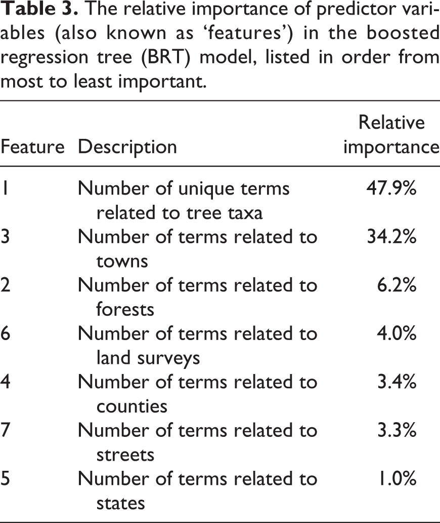
The BRT model produced an AUC value of 0.99 when calculated on the training dataset (Section II.1.3). Relative importance of model predictor variables is presented in Table 3. Features 1 and 3 (i.e. the number of unique terms related to tree taxa, and to towns, respectively) both exhibited positive curvilinear relationships with the probability of a text chunk containing a FCD, with local maxima in probability at approximately eight mentions of unique tree taxa and 10 mentions of town-related terms (see Table 3 and Figure 3). Features 5, 6, and 7 each exhibited generally negative relationships with probability, whereas Features 2 and 4 showed relationships that were difficult to interpret using partial dependence plots. The most important two-way interaction was between Feature 1 and Feature 3 (Figure 3). When calibrating thresholds for classifying text chunks as containing or not containing an FCD, a predicted probability of 13.25% was selected as Threshold 1 (to maximize the sum of true positive and true negative rates), and 0.80% was selected as Threshold 2 (to achieve a recall of 100%).

Table 3.

The relative importance of predictor variables (also known as ‘features’) in the boosted regression tree (BRT) model, listed in order from most to least important.

Feature	Description	Relative importance
1	Number of unique terms related to tree taxa	47.9%
3	Number of terms related to towns	34.2%
2	Number of terms related to forests	6.2%
6	Number of terms related to land surveys	4.0%
4	Number of terms related to counties	3.4%
7	Number of terms related to streets	3.3%
5	Number of terms related to states	1.0%

Figure 3.

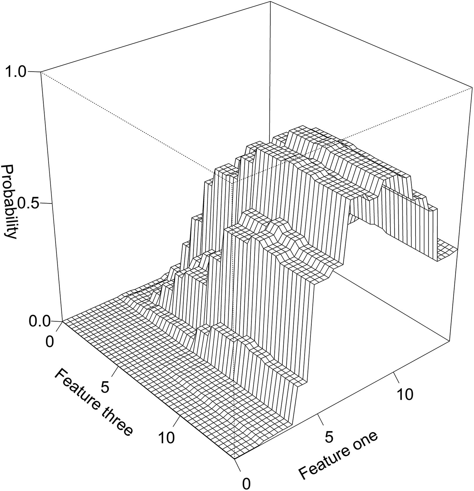
A partial dependence plot showing the probability of a text chunk containing a forest compositional description (FCD) at the town resolution, as predicted by the boosted regression tree (BRT) model. The plot shows the most important two-way interaction, between Feature 1 (number of unique terms related to tree taxa) and Feature 3 (number of terms related to towns). The feature axes indicate the number of words in the text chunk that match key terms within that feature (Table 1). To create this plot, the values of other predictor variables (also known as ‘features’) are held at their mean value, as the values of the two variables in the plot are varied.

When evaluated upon text chunks with two or more unique taxa mentions in the test dataset, the BRT model yielded an AUC value of 0.96 using all text chunks (n = 7198), and 0.97 using text chunks with the highest predicted probabilities out of each pair of overlapping text chunks (n = 3687). The remaining results of this section pertain to the latter set of text chunks. The next two paragraphs describe model evaluation when Threshold 1 was applied, whereas the final paragraph of this section pertains to when Threshold 2 was applied. Results for all threshold-dependent evaluation statistics, calculated upon training and test datasets and using both Threshold 1 and Threshold 2, are shown in Table 4. As one example of the model predictions, the model predicted that the text shown in Figure 1 possessed a 96.1% (using the first two paragraphs) to 98.4% (using the second two paragraphs) probability of containing a FCD at township resolution.

Table 4.

The predictive performance of the boosted regression tree (BRT) model using three evaluation statistics. Threshold 1 was selected to maximize the sum of true positive and true negative rates, and Threshold 2 was selected to ensure total recall of forest compositional descriptions (FCDs), when the model was applied to the training dataset. For the test dataset, statistics in this table were calculated using text chunks with the highest predicted probability within each pair of overlapping text chunks (Section II.1.4).

	Training dataset		Test dataset
	Threshold 1	Threshold 2	Threshold 1	Threshold 2
Accuracy	97.5%	89.4%	94.2%	81.7%
Precision	65.0%	29.3%	73.2%	41.3%
Recall	95.0%	100%	87.6%	97.5%

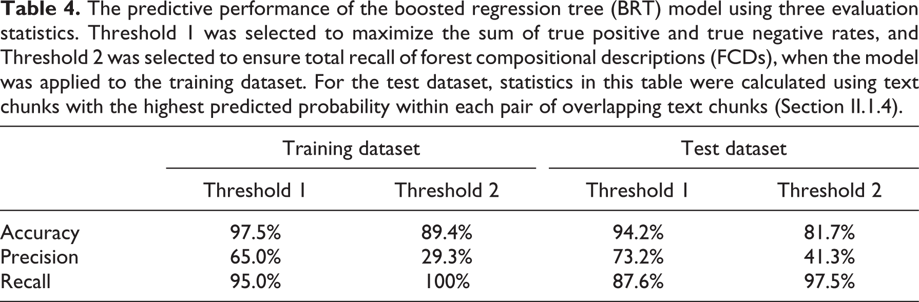
Using Threshold 1, the model yielded a precision of 73.2%, representing the percent of text chunks from the test dataset classified as containing a FCD that actually contained a FCD. The model yielded a recall of 87.6%, representing the percent of text chunks with FCDs that were correctly classified as containing a FCD. Precision and recall statistics for specific counts of unique tree taxa (counted using the Python script; Section II.1.2) are presented in Figure 4; the model generally yielded 90–100% recall when five or more unique tree taxa were mentioned. The BRT model predicted that 571 out of 3687 text chunks (15.5%) with two or more unique taxa contained a FCD. These 571 text chunks represented approximately 0.1% of the total text within the 174 volumes of Ohio county histories.

Figure 4.

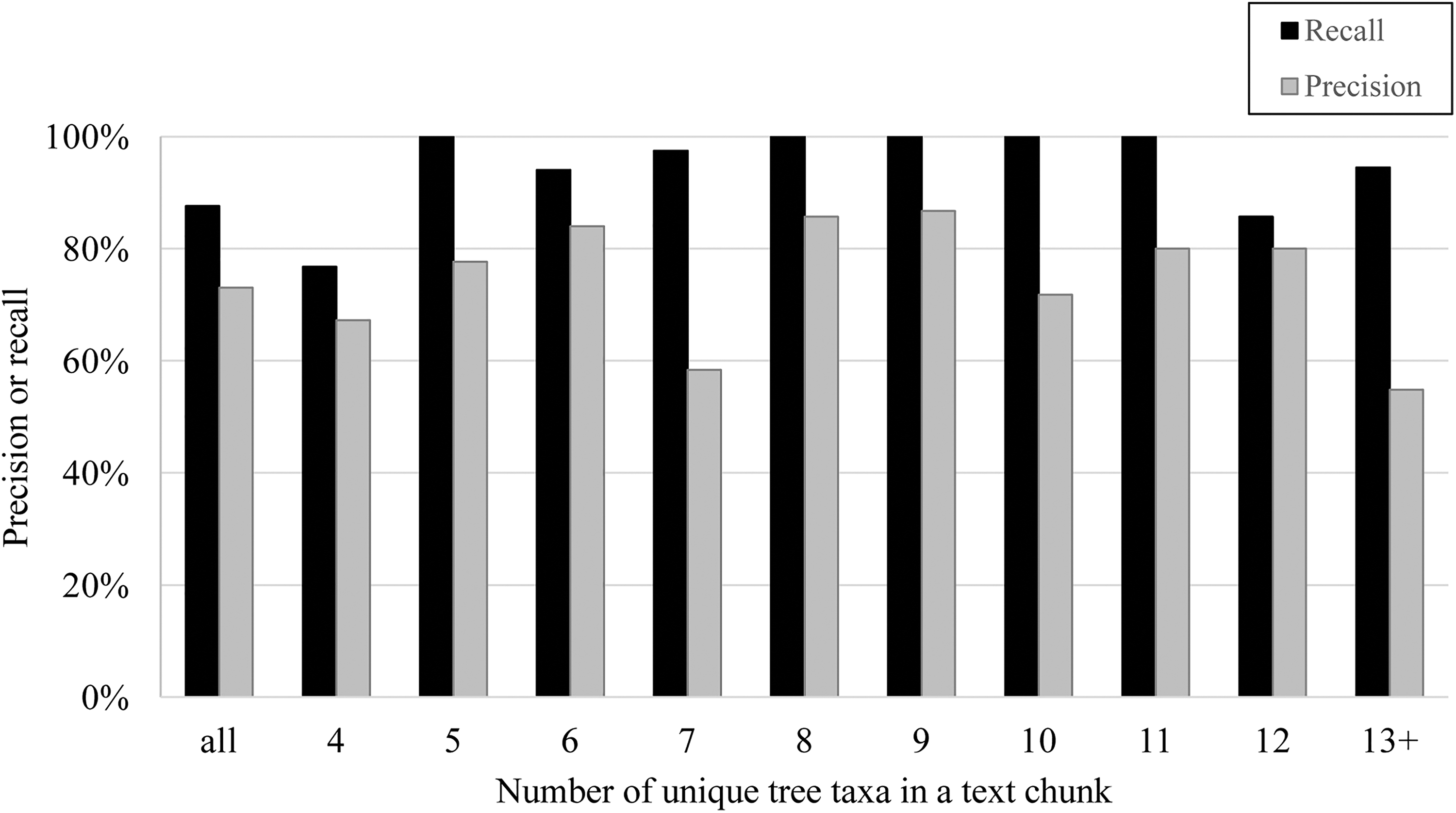
Precision and recall across different numbers of unique taxa in a forest compositional description (FCD) in the test dataset (i.e. Ohio county histories), using text chunks with the highest predicted probability per pair of overlapping text chunks (Section II.1.4), and using Threshold 1 (maximizing the sum of true positive and true negative rates). The number of unique taxa in this figure was calculated using the number of unique mentions counted by the Python script (Section II.1.2).

Also using Threshold 1, 59 text chunks were incorrectly classified as not containing an FCD. Compared to all FCDs together (see next section), FCDs within text chunks generally contained fewer unique mentions to tree taxa. A total of 50 out of 59 (85%) text chunks containing FCDs that were misclassified mentioned four or fewer unique taxa. The absence of terms related to towns (Table 1) appears to have also contributed to incorrect classifications for text chunks mentioning six or more unique taxa; just one out of nine text chunks with more than four unique taxa mentioned contained one or more such town terms. OCR errors generally did not appear to be implicated in the incorrect classification of these text chunks (e.g. by leading to an incorrect spelling of a tree taxon, a lowered count of total tree taxa mentioned, and a lower predicted probability).

The following results pertain to model evaluation when applying Threshold 2 (i.e. recall = 100% using the training dataset). A total of 1126 out of 3687 text chunks (30.5%) with two or more unique taxa were predicted as containing an FCD in the test dataset; 465 out of these 1126 (precision = 41.3%) actually contained one, whereas 465 out of 477 (recall = 97.5%) of text chunks identified as containing an FCD were classified by the model as such. Similar to results observed when using Threshold 1, when using Threshold 2 the 15 misclassified text chunks that contained FCDs exhibited fewer unique mentions of tree taxa. The 1126 text chunks classified by the model as containing an FCD represented approximately 0.3% of the total text within the 174 volumes of Ohio county histories.

2. FCDs

Section III.2.1 reports the basic characteristics of FCDs. Section III.2.2 reports the results of comparisons between FCDs and PLSRs.

2.1. Basic characteristics of FCDs

Ohio county histories contained 477 FCDs at township resolution, of which 411 were unique FCDs (i.e. not derivative of earlier works). Figure 5 maps the locations of all FCDs, irrespective of whether the BRT model classified text as containing an FCD for a given location. A mean of 2.4 unique FCDs were present per volume of county history. Descriptions represented approximately 365 townships (26.7% of townships) covering 27.1% of the total area of Ohio. Of the unique FCDs, approximately 275 (66.9%) described ‘original’ forest composition prior to or at the start of Euro-American settlement, and 268 (65.2%) summarized forest composition as one aggregate description for the entire township (Section I). Of the unique FCDs, 179 (44.6%) were both descriptions of ‘original’ forest composition and summarized for the entire township (e.g. Figures 1 and 5). These 179 FCDs mentioned a mean of 6.9 unique taxa (standard deviation = 3.0) as counted by the Python script (Section II.1.2), and a mean of 8.0 unique taxa (standard deviation = 4.3) as counted during human review of FCDs.

Figure 5.

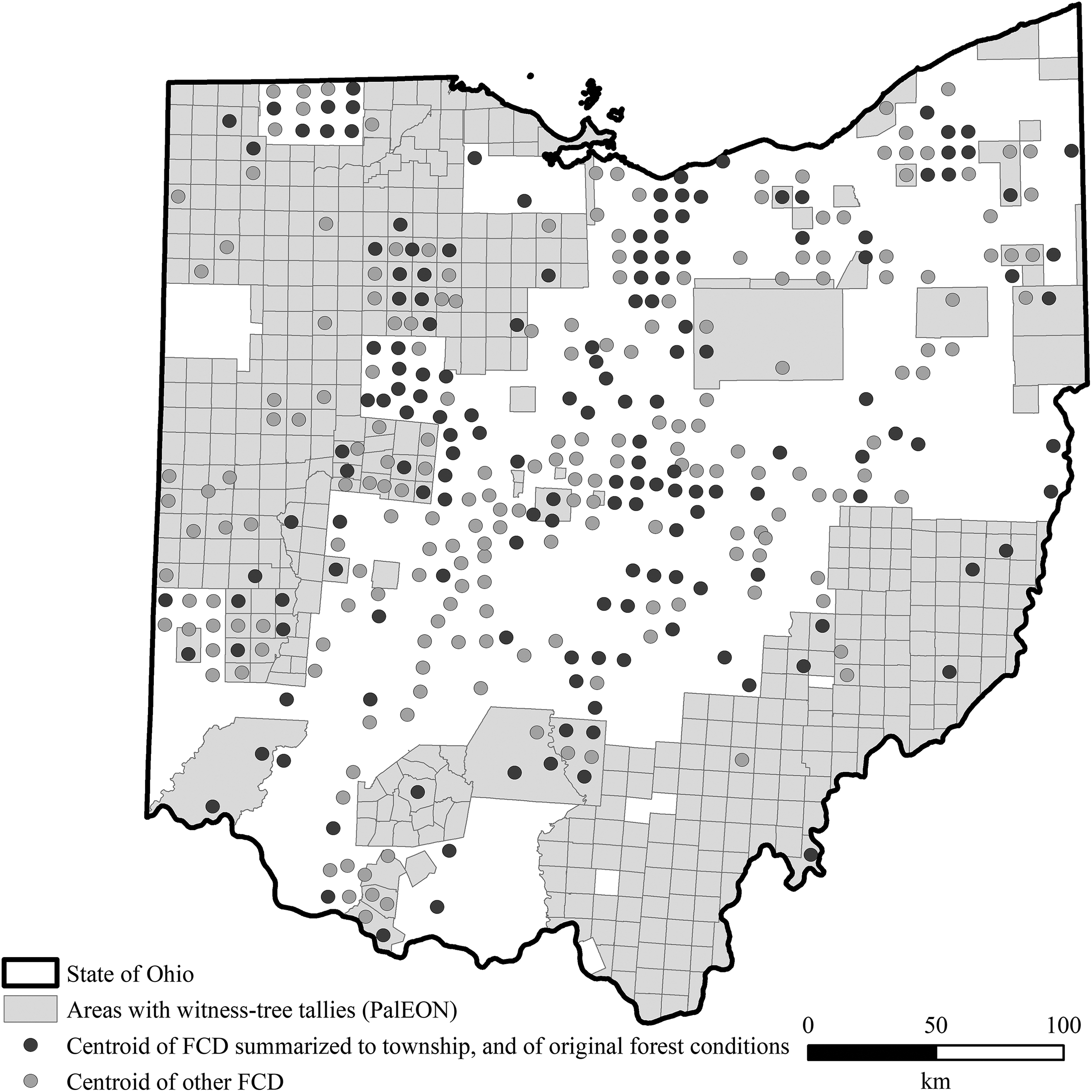
Centroids of townships with at least one forest compositional description (FCD), and areas with witness-tree tallies from presettlement land survey records (PLSRs; Paciorek et al., 2016). FCDs were manually mapped using a 1920 township data layer (University of Minnesota, 2010). A small portion (<10) of FCDs were not locatable (potentially due to changes in township names and/or dissolution) and, therefore, not mapped. ‘Other’ FCDs mapped were descriptions of forest composition that were either not summarized to the township, or were subdivided by soil, topographic, or other conditions (Section I).

2.2. Comparison of FCDs with PLSRs

Table 5 shows the results of t-tests assessing if a taxon’s relative abundance reported in PLSRs was different at locations where FCDs (n = 179) mentioned versus did not mention the taxon. Out of 16 taxa, seven showed significant differences in relative abundance between FCD locations where the taxon was mentioned versus not mentioned. Beech (significant) and oak (not significant) showed the greatest differences (by percentage points of relative abundance) between locations that did versus did not mention the taxon. Of taxa with at least 10 FCDs that did or did not mention the taxon, cherry (not significant) and walnut (not significant) showed the smallest differences in relative abundances.

Table 5.

Results of t-tests for significant differences between relative abundance (Paciorek et al., 2016) at locations with versus without a taxon mentioned in forest compositional descriptions (FCDs) in the State of Ohio. Five out of 23 taxa had one or no mentions in FCDs and were therefore omitted from this analysis. See online supplementary material for more information on how taxa were grouped into the categories shown below.

Taxon common name	Number of FCDs with mention	Number of FCDs without mention	Mean relative abundance, where mentioned	Mean relative abundance, where not mentioned	p-value	Sig.
Ash	107	58	8.5%	5.5%	<0.001	**
Basswood	33	132	2.9%	1.9%	0.033	*
Beech	114	51	25.0%	16.0%	<0.001	**
Birch	2	163	0.1%	0.0%	0.265
Cherry	42	123	0.3%	0.3%	0.497
Chestnut	27	138	1.7%	0.5%	<0.001	**
Dogwood	8	157	2.1%	1.2%	0.219
Elm	91	74	7.4%	6.1%	0.034	*
Gum	7	158	1.5%	0.7%	0.075
Hickory	120	45	10.2%	8.1%	0.002	**
Ironwood	6	159	1.1%	1.4%	0.245
Maple	131	34	13.8%	11.0%	0.001	**
Oak	153	12	28.2%	23.9%	0.122
Other hardwood	62	103	3.9%	3.3%	0.107
Pine	4	161	1.3%	0.1%	0.189
Poplar	66	99	1.6%	1.2%	0.017	*
Spruce	2	163	0.0%	0.0%	<0.001	**
Walnut	123	42	1.3%	1.2%	0.342

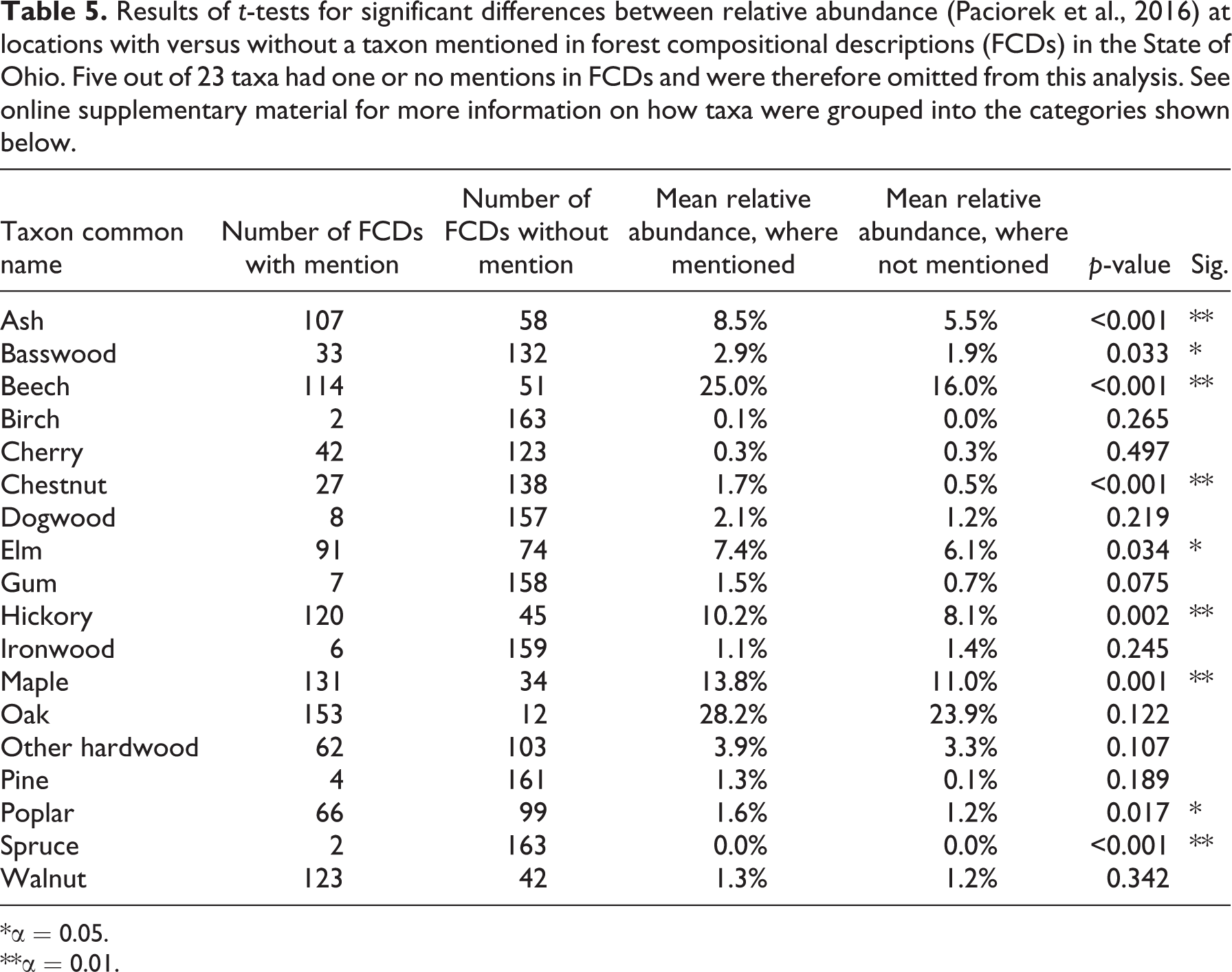
*α = 0.05.

**α = 0.01.

Comparisons between prevalence rank in FCDs and abundance rank in PLSRs generally showed strong correlations. After selecting FCDs in Ohio that were both descriptions of ‘original’ forest composition and summarized for the entire township (n = 179), and then removing one FCD for each township with more than one FCD, 165 FCDs remained. Comparing the prevalence rank of taxa for these FCDs with the abundance rank of taxa in PLSRs (Section II.2.2) yielded an R² value of 0.82. An R² value of 0.83 was produced when understory trees (i.e. dogwood and ironwood) were omitted, and when understory trees plus the ‘other hardwoods’ were omitted. Using all FCDs in Ohio, the top five most prevalent taxa in FCDs were oak, maple, walnut, hickory, and beech; the top five most abundant taxa in PLSRs were oak, beech, maple, hickory, and ash (Figure 6). The taxa with the biggest differences between FCDs and PLSRs were generally walnut and cherry; these taxa had higher prevalence ranks in FCDs than abundance ranks in PLSRs. In comparisons between prevalence rank determined from randomly selected FCDs, and abundance rank from PLSRs, R² values were generally maximized with approximately 100 or more FCDs (Figure 7).

Figure 6.

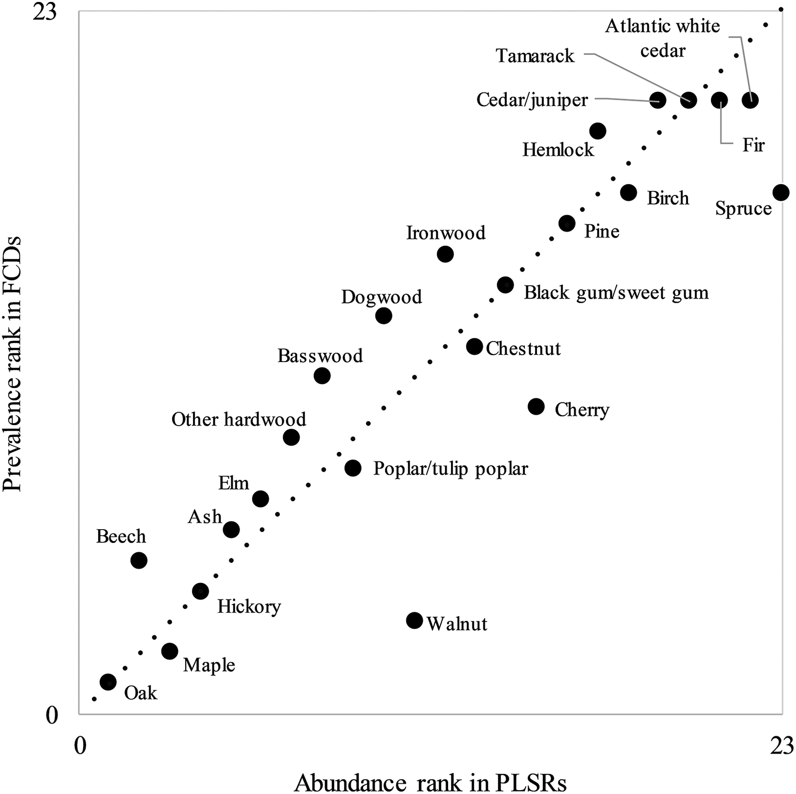
Prevalence rank of taxa in forest compositional descriptions (FCDs), versus abundance rank estimated using interpolated relative abundance data (Paciorek et al., 2016), for the state of Ohio. In this figure, abundance rank was estimated by first calculating for each taxon its mean relative abundance in Ohio using interpolated abundance data, and then assigning its abundance rank compared to other taxa. The dotted line is a 1:1 line; the R² value for the comparison shown was 0.82. Note that four taxa were not mentioned in FCDs and are ranked last in prevalence rank.

Figure 7.

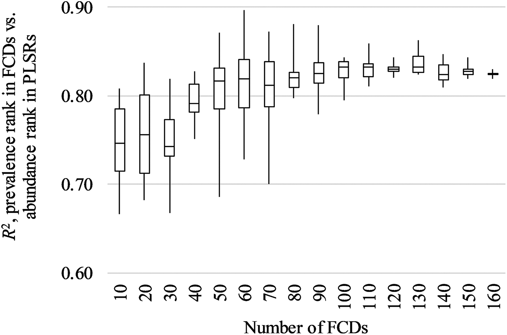
Boxplot of R² values of prevalence rank of taxa in forest compositional descriptions (FCDs) versus abundance rank based on presettlement land survey records (PLSRs; Paciorek et al., 2016), across varying numbers of FCDs. The median, 25th/75th percentile (boxes), and minimum and maximum (whiskers) R² values are shown. Varying numbers (10 to 160) of FCDs were randomly selected and the prevalence rank of each taxon was determined, and then compared to abundance rank; this process was repeated numerous times to produce the boxplot shown. Prevalence rank was compared to estimates of abundance rank, using relative abundance values from interpolated data for all of Ohio.

In the regional-scale comparison of FCDs to other distributional data, FCDs were discovered for 302 unique towns across 10 states using the BRT model; FCDs from Delaware, Maryland, Virginia, and West Virginia were excluded (Figure 2) because PLSR data were not available for these states. Figure 8 presents various spatial outputs and comparisons: the locations of FCDs, species mentions in FCDs, Little and Viereck’s species ranges within the 10-state region (1971), and interpolated relative abundances (Paciorek et al., 2016).

Figure 8.

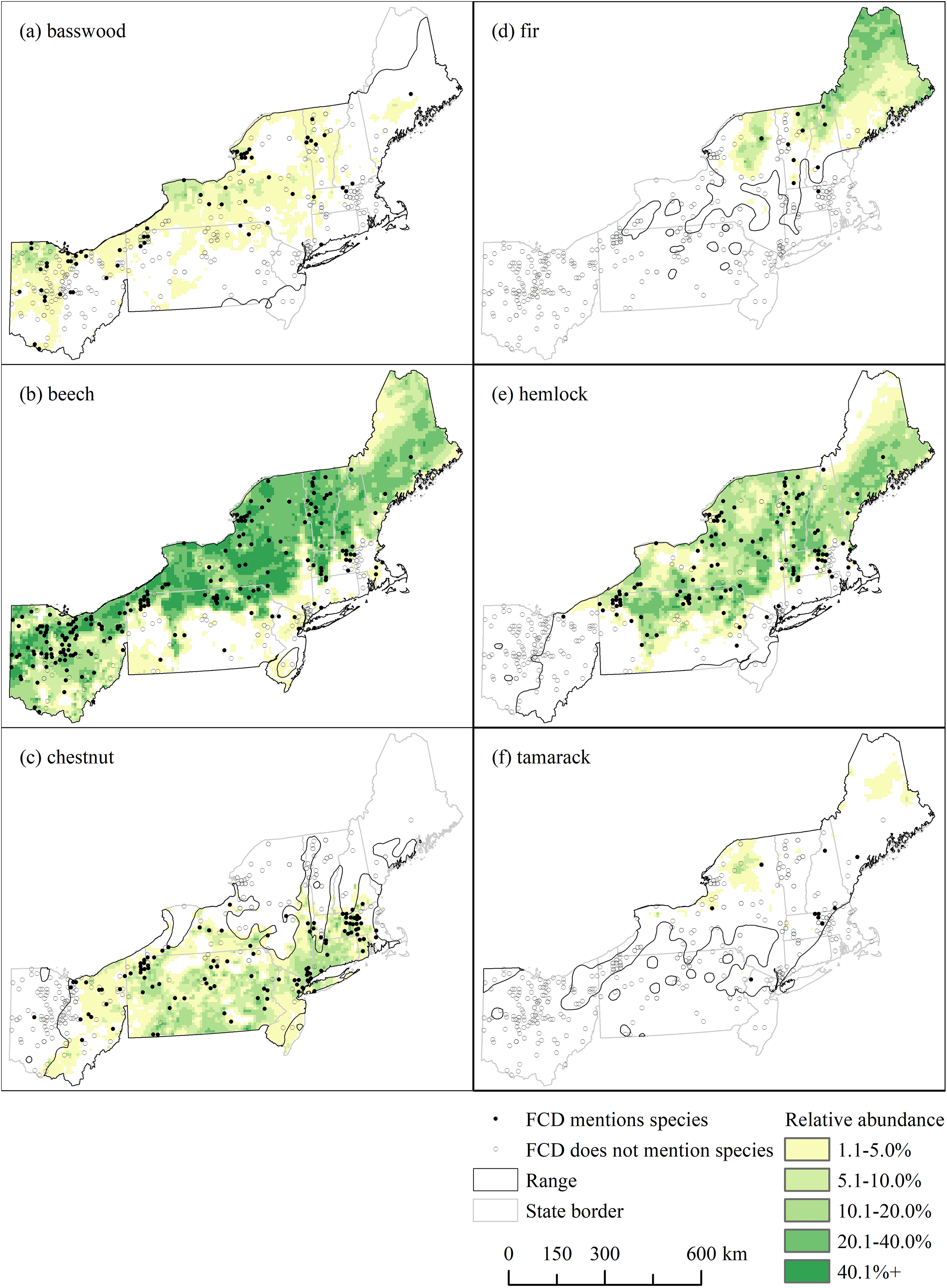
Comparisons between mentions of species in forest compositional descriptions (FCDs), species ranges within the study area (Little and Viereck, 1971), and interpolated relative abundances (Paciorek et al., 2016).

IV. Discussion

The results demonstrate the potential of IR methods to develop novel datasets over large geographic areas, in order to corroborate existing historical datasets and provide spatial coverage of historic phenomena where other records do not exist. The results also more generally offer methodological considerations for other physical geography applications with historical foci. Section IV.1 discusses the overall usefulness of the IR approach in this study, and Section IV.2 discusses the usefulness of the IR approach more specifically towards this study’s application.

1. How useful are IR approaches for historical physical geography applications?

This study shows promise for accelerating the search for historical information from collections of digitized documents for physical geography studies across large geographic areas, alleviating barriers presented by manually searching and reading documents (Edmonds, 2005). This study produced a ranking model that yielded a high recall and was generalizable to county histories in other geographic areas (Table 4). The model produced a high recall for FCDs both overall and across varying numbers of unique tree taxa mentioned (Figure 4), with false negatives occurring for FCDs with purportedly less ecological value (i.e. fewer numbers of unique tree taxa described). Given the results, the use of Threshold 2 (i.e. achieving near-total recall) is promoted over Threshold 1 (i.e. maximizing overall accuracy considering both positive and negative classifications). With a lower prediction threshold that classified more text chunks as containing an FCD, the model involving Threshold 2 still produced a precision of 41.3%, meaning that during human review of text classified as containing an FCD, roughly four out of 10 text chunks would contain pertinent information. Using this threshold, nearly all FCDs in the test dataset were discovered, yielding a recall of 97.5% and creating a subset of just 0.3% of text from the county histories for human review. The importance of predictor variables (Table 3), and the relationships between predictor variables and probabilities (e.g. Figure 3), were generally consistent with expectations.

Four methodological considerations are noted here. First, and most closely related to this study’s application, future applications of IR ranking models for the discovery of FCDs in other geographical locations should modify lists of taxa that are searched for (e.g. Table 1), both to account for different taxa in those locations and for differences in common names used to describe taxa. Second, future studies could explore additional predictors or predictor selection methods, such as term frequencies (versus raw totals) or heuristics to identify important features of texts containing pertinent information (e.g. the term frequency-inverse document frequency measure; Jones, 1972). Third, this study took a supervised approach towards developing a model for ranking text based upon relevance to a topic, but other supervised and unsupervised topic modeling approaches from TM (Blei et al., 2003; Hofmann, 1999) could present alternative ways to assign different ‘topics’ to portions of text. For example, a researcher focusing on a keyword (e.g. a species, or a natural event such as a flood) could use TM and IR methods to automate the classification of portions of text that mention the keyword into multiple relevant and non-relevant topics. Fourth, this study acquired digitized historical documents through manual downloading. Future approaches could automate the selecting and downloading of appropriate documents to acquire even larger collections of documents, using IR approaches that use document metadata to retrieve documents pertinent to a search (e.g. Kim et al., 2005), and programming packages to automate the downloading of documents from Internet sources with freely available documents (e.g. Petrov, 2016).

Furthermore, this study’s methods were applied to a common biogeographical pursuit – that is, mapping past taxon distributions. Adaptations of this method could be modified for other physical geography applications, such as in geomorphology and climatology. Applications made apparent through the incidental discovery of topics in county histories include accounts of notable droughts and floods. As mentioned, studies have compared qualitative historical accounts of regional-scale disturbances to growth-release events recorded in tree-rings (Pederson et al., 2014), and other sources have compiled accounts of flooding from historical written sources (e.g. Brázdil et al., 1999). A cursory search revealed that county histories in this study contained descriptions of notable droughts in 1755, 1760, and 1779 in Massachusetts; and accounts of flooding along the Ohio River back to 1773 and the Susquehanna River back to 1744.

2. Are FCDs useful?

Despite apparent biases and ambiguities in FCDs discussed below, results suggest that large collections of FCDs are useful for understanding original forest composition over broad regions, in turn demonstrating the usefulness of the IR approach presented. With approximately 100+ FCDs (Figure 7), a strong relationship (R² = 0.82) existed between the prevalence rank of carefully selected FCDs and the abundance rank in PLSRs, suggesting that the relative abundance of a taxon is related to the frequency with which it is mentioned in a collection of FCDs. This correlation was apparent even though the distribution of FCDs across Ohio was not even (Figure 5); the distribution of county histories that provided FCDs (Figure 2) appears vaguely correlated with patterns in historic and current human population in Ohio. Both population patterns and regional differences in the popularity of county histories (Way, 2010) may, therefore, dictate the availability of historical sources for discovering FCDs. However, larger collections of FCDs where present appear to minimize the idiosyncrasies and biases of single FCDs and produce a proxy of abundance rank.

Further supporting their use over broad areas, results suggest that mentions of species in FCDs can recreate general patterns in original species ranges insofar as where species are more abundant. As suggested by Figure 8, species mentions appeared to be more correlated with relative abundances (Paciorek et al., 2016) than distributional ranges (Little and Viereck, 1971). For example, mentions of beech in FCDs (Figure 8(b)) generally occurred in areas of higher interpolated relative abundance in Ohio, into northern Pennsylvania, and northeasterly. Conversely, beech was less mentioned and less abundant in southern Pennsylvania and in coastal areas. As another example, mentions of basswood in FCDs (Figure 8(a)) generally occurred in areas of higher abundance but less frequently given its overall lower abundance compared to beech. The differences in patterns between the FCDs and available witness-tree data from PLSRs further suggest that FCDs produced by the IR approach can fill in geographic gaps in knowledge where other historical data do not exist (Figure 5).

While large collections of FCDs may imply relative abundance rank over regions, other analyses suggest that FCDs should be interpreted with some caution. Taxonomic biases and ambiguities, always of concern when using historical accounts (Edmonds, 2005; Whitney, 1996), are worth noting. The t-tests comparing relative abundance of a taxon at locations where the taxon was mentioned versus not mentioned in FCDs in Ohio (Table 5), and plots of prevalence rank in FCDs versus abundance rank in PLSRs (Section III.2.2; Figure 6) both suggest biases towards mentioning large and economically valuable tree taxa (e.g. walnut and cherry) and against mentioning smaller tree taxa (e.g. dogwood and ironwood). An illustrative example is walnut, whose relative abundance in PLSR data was only 1.3% at FCD locations where mentioned (Table 5), and whose prevalence rank in FCDs was third versus its abundance rank in PLSRs of seventh (Figure 6). With these results, an interpretation of bias in FCDs is favored over error in PLSRs, given the general plausibility of such biases; yet, at least one FCD explicitly mentioned walnut as being most abundant. Biases aside, the FCDs still appear useful for offering a means of validating PLSR data, given the strong correlation between prevalence rank and abundance rank. It is also expected that if similar t-tests (Table 5) were performed over larger geographic areas with greater variation in taxon abundances (Figure 8), differences between relative abundance where a taxon was or was not mentioned in FCDs would be more pronounced.

Additional issues surrounded taxonomic ambiguities, of which two examples are highlighted. First, a single reference to ‘chestnut’ appeared in western Ohio (Figure 8(c)); this reference is either a discontinuous portion of the Castanea dentata range not mapped by Little and Viereck (1971), a reference to ‘buckeye’ (Aesculus glabra) or the European ‘horse chestnut’ (Aesculus hippocastanum), or a reference to chestnut oak (Quercus montana). Second, mentions of ‘spruce’ (Picea spp.) in Ohio may instead have referred to hemlock (Tsuga canadensis) since the latter is occasionally known as ‘spruce pine’ (Cogbill et al., 2002) and other variants; grouping ‘spruce’ with ‘hemlock’ would have strengthened correlations between prevalence rank and abundance rank (e.g. Figure 6).

Collectively, the results warrant the continued study of FCDs alongside PLSRs, while maintaining an awareness of potential biases in FCDs. Two pursuits are highlighted. First, collections of additional FCDs over broad geographic areas could be pursued to infer abundance rank of taxa from prevalence rank, and to interpolate general areas with higher relative abundances, to then compare with PLSRs. Second, explicit mentions of the most abundant tree taxa in FCDs could furthermore be compared to the most abundant taxa in PLSRs.

V. Conclusion

This study manifested the potential for applying IR methods towards the development of a custom search engine to discover information in digitized historical documents pertinent to a physical geography application. Future work should apply such methods towards other pursuits within physical geography to further test its efficacy. Such methods have the potential to complement and corroborate other historical or quantitative methods, and to motivate the development of novel datasets over large geographic areas from digitized historical documents.

Supplementary material

Supplemental Material, 08b_Table_taxa_common_names_v3 - Information retrieval in physical geography: A method to recover geographical information from digitized historical documents

Supplemental Material, 08b_Table_taxa_common_names_v3 for Information retrieval in physical geography: A method to recover geographical information from digitized historical documents by Stephen J. Tulowiecki in Progress in Physical Geography: Earth and Environment

Footnotes

Acknowledgements

SJT thanks Preston F Seader for his assistance in assembling figures and collecting data. SJT also thanks Internet Archive and its volunteers for providing the county histories used in this paper.

Declaration of Conflicting Interests

The author(s) declared no potential conflicts of interest with respect to the research, authorship, and/or publication of this article.

Funding

The author(s) received no financial support for the research, authorship, and/or publication of this article.

ORCID iD

Stephen J Tulowiecki

Supplementary material

Supplementary material for this article is available online.

References

Black

Ruffner

Abrams

(2006) Native American influences on the forest composition of the Allegheny Plateau, northwest Pennsylvania. Canadian Journal of Forest Research-Revue Canadienne De Recherche Forestiere 36: 1266–1275.

Blei

Jordan

(2003) Latent Dirichlet Allocation. Journal of Machine Learning Research 3: 993–1022.

Bourdo

Jr (1956) A review of the General Land Office survey and of its use in quantitative studies of former forests. Ecology 37: 754–768.

Brázdil

Glaser

Pfister

. (1999) Flood events of selected European rivers in the sixteenth century. Climatic Change 43: 239–285.

Broder

Carmel

Herscovici

. (2003) Efficient query evaluation using a two-level retrieval process. In: Ophir

Frieder

(ed) CIKM ‘03 proceedings of the twelfth international conference on information and knowledge management, New Orleans, LA, USA, 3–8 November 2003, New York, NY USA: Association for Computing Machinery, 426–434.

Chenoweth

(2006) A reassessment of historical Atlantic basin tropical cyclone activity, 1700-1855. Climatic Change 76: 169–240.

Cogbill

Burk

Motzkin

(2002) The forests of presettlement New England, USA: Spatial and compositional patterns based on town proprietor surveys. Journal of Biogeography 29: 1279–1304.

Comber

Fisher

Wadsworth

(2015) Text mining analysis of land cover semantic overlap. In: Ahlqvist

Varanka

Fritz

. (eds) Land Use and Land Cover Semantics: Principles, Best Practices, and Prospects. New York: CRC Press, 191–210.

Curry

(1915) History of Union County, Ohio: Its People, Industries and Institutions. Indianapolis, IN: Bowen & Co.

10.

Edmonds

(2005) The pleasures and pitfalls of written records. In: Egan

Howell

(eds) The Historical Ecology Handbook: A Restorationist’s Guide to Reference Ecosystems. Washington, DC: Island Press, 73–99.

11.

Elith

Leathwick

Hastie

(2008) A working guide to boosted regression trees. Journal of Animal Ecology 77: 802–813.

12.

Esri (2017) ArcGIS 10.5.1. Redlands, CA, USA.

13.

Fawcett

(2006) An introduction to ROC analysis. Pattern Recognition Letters 27: 861–874.

14.

Feldman

Sanger

(2007) The Text Mining Handbook: Advanced Approaches in Analyzing Unstructured Data. New York: Cambridge University Press.

15.

Filby

(1985) A Bibliography of American County Histories. Baltimore, MD: Genealogical Publishing Company.

16.

Fisher

Knowlton

Brainard

. (2011) Differences among major taxa in the extent of ecological knowledge across four major ecosystems. PLoS ONE 6: e26556.

17.

Franklin

Miller

(2009) Mapping Species Distributions: Spatial Inference and Prediction. New York: Cambridge University Press.

18.

Friedman

(2001) Greedy function approximation: A gradient boosting machine. The Annals of Statistics 29: 1189–1232.

19.

Friedman

(2002) Stochastic gradient boosting. Computational Statistics & Data Analysis 38: 367–378.

20.

Google (2017) Google Books. Available at: https://books.google.com/ (accessed 10 April 2018).

21.

Grabowski

Gurnell

(2016) Using historical data in fluvial geomorphology. In: Kondolf

Piégay

(eds) Tools in Fluvial Geomorphology. Hoboken, NJ: John Wiley & Sons. 77–101.

22.

Hammond

(2008) PythonWin – Python IDE and GUI Framework for Windows. BeOpen.com, Corporation for National Research Initiatives, and Stichting Mathematisch Centrum.

23.

HathiTrust (2017) HathiTrust Digital Library. Available at: https://www.hathitrust.org/ (accessed 10 April 2018).

24.

Hijmans

Phillips

Leathwick

. (2013) Dismo: Species distribution modeling. R package version 0.8-17. Available at: http://CRAN.R-project.org/package=dismo (accessed 10 April 2018).

25.

Hofmann

(1999) Probabilistic latent semantic analysis. In: Laskey

Kathryn B

Henri

Prade

(eds) Proceedings of uncertainty in artificial intelligence, UAI ‘99, Stockholm, Sweden, July 30–August 1, 1999, San Francisco, California USA: Morgan Kaufmann, 289–296.

26.

Hooke

Kain

RJP

(1982) Historical Change in the Physical Environment: A Guide to Sources and Techniques. London: Butterworth Scientific.

27.

Internet Archive (2017) About the Internet Archive. Available at: https://archive.org/about/ (accessed 10 April 2018).

28.

Joachims

(2002) Optimizing search engines using clickthrough data. In: Zaïane

Osmar R

(ed) KDD ‘02 proceedings of the eighth ACM SIGKDD international conference on knowledge discovering and data mining, Edmonton, Alberta, Canada, 23–25 July 2002, New York, NY USA: ACM, 133–142.

29.

Jones

(1972) A statistical interpretation of term specificity and its application in retrieval. Journal of Documentation 28: 11–21.

30.

Kim

Myaeng

Yoo

J-M

(2005) A hybrid information retrieval model using metadata and text. In: Fox

Edward A

Neuhold

Erich J

Pimrumpai

Premsmit

Wuwongse

Vilas

ICADL’05 proceedings of the 8th international conference on Asian digital libraries, Bangkok, Thailand, 12–15 December 2005, New York, NY USA: Springer, 232–241.

31.

Kronenfeld

Wang

Y-C

(2007) Accounting for surveyor inconsistency and bias in estimation of tree density from presettlement land survey records. Canadian Journal of Forest Research-Revue Canadienne De Recherche Forestiere 37: 2365–2379.

32.

Little

Viereck

(1971) Atlas of United States Trees. Washington, DC: US Department of Agriculture.

33.

Meyerink

(1998) Printed Sources: A Guide to Published Genealogical Records. Salt Lake City, UT: Ancestry Incorporated.

34.

Ohio Department of Natural Resources (2002) Ohio original land subdivisions. Available at: http://apps.ohiodnr.gov/geodata/Statewide/ODNR_TOWNSHIP.zip (accessed 10 April 2018).

35.

Paciorek

Goring

Thurman

. (2016) Statistically-estimated tree composition for the northeastern United States at the time of Euro-American settlement. PLoS ONE 11: e0150087.

36.

Pederson

Dyer

McEwan

. (2014) The legacy of episodic climatic events in shaping temperate, broadleaf forests. Ecological Monographs 84: 599–620.

37.

Petrov

(2016) urllib3. Python package version 1.22. Available at: https://pypi.python.org/pypi/urllib3 (accessed 10 April 2018).

38.

Prasad

Iverson

(2003) Little’s range and FIA importance value database for 135 eastern US tree species. Available at: http://www.fs.fed.us/ne/delaware/4153/global/littlefia/index.html (accessed 10 April 2018).

39.

ProQuest (2017) HeritageQuest Online. Available at: http://www.heritagequestonline.com/hqoweb/library/do/login (accessed 10 April 2018).

40.

R Development Core Team (2011) R: A Language and Environment for Statistical Computing. Vienna: R Foundation for Statistical Computing.

41.

Ridgeway

(2013) gbm: Generalized Boosted Regression Models. R package version 2.1. Available at: http://CRAN.R-project.org/package=gbm (accessed 10 April 2018).

42.

Ruffner

(2006) Understanding the evidence for historical fire across eastern forests. In: Dickinson

(ed) Fire in Eastern Oak Forests: Delivering Science to Land Managers, Proceedings of a Conference. Columbus, OH: USDA Forest Service, Northern Research Station, 40–48.

43.

Stewart

(2002) Forgotten Fires: Native Americans and the Transient Wilderness. Norman, OK: University of Oklahoma Press.

44.

Tamaddoni-Nezhad

Milani

Raybould

. (2013) Construction and validation of food webs using logic-based machine learning and text mining. In: Woodward

Bohan

(eds) Advances in Ecological Research, Vol 49: Ecological Networks in an Agricultural World. San Diego, CA: Elsevier Academic Press Inc, 225–289.

45.

Tulowiecki

(2015) Assessing Native American Influences upon Pre-European Tree Species Composition in Western New York: An Approach Using Original Land Survey Records and Species Distribution Models. Buffalo, NY: Department of Geography, University at Buffalo, 253.

46.

Tyree

Weinberger

Agrawal

(2011) Parallel boosted regression trees for web search ranking. In: Sadagopan

Elisa

Bertino

Ravi

Kumar

WWW ‘11 proceedings of the 20th international conference on world wide web, Hyderabad, India March 28-April 1 2011, New York, NY USA: Association for Computing Machinery, 387–396.

47.

University of Michigan (2007) Michigan County Histories and Atlases Digitization Project. Available at: http://quod.lib.umich.edu/m/micounty/ (accessed 10 April 2018).

48.

University of Minnesota (2010) NHGIS Data Finder. Available at: https://data2.nhgis.org/main (accessed 10 April 2018)

49.

US Department of Agriculture (2017) Tree species in the Climate Change Tree Atlas. Available at: http://www.fs.fed.us/nrs/atlas/tree/resources/spp-list.php (accessed 10 April 2018).

50.

Wadsworth

Balzter

Gerard

. (2009) An environmental assessment of land cover and land use change in Central Siberia using Quantified Conceptual Overlaps to reconcile inconsistent data sets. Journal of Land Use Science 3: 251–264.

51.

Wang

Y-C

(2005) Presettlement land survey records of vegetation: Geographic characteristics, quality and modes of analysis. Progress in Physical Geography 29: 568–598.

52.

Way

(2010) American county histories: Their uses, usability, sources and problems with access. Available at: http://www.accessible-archives.com/collections/american-county-histories/a-white-paper-american-county-histories/ (accessed 10 April 2018).

53.

Weiss

Indurkhya

Zhang

(2015) Fundamentals of Predictive Text Mining. London: Springer-Verlag.

54.

Whitney

(1996) From Coastal Wilderness to Fruited Plain: A History of Environmental Change in Temperate North America, 1500 to the Present. New York: Cambridge University Press.

55.

Williams

Baker

(2010) Bias and error in using survey records for ponderosa pine landscape restoration. Journal of Biogeography 37: 707–721.

Supplementary Material

Please find the following supplemental material available below.

For Open Access articles published under a Creative Commons License, all supplemental material carries the same license as the article it is associated with.

For non-Open Access articles published, all supplemental material carries a non-exclusive license, and permission requests for re-use of supplemental material or any part of supplemental material shall be sent directly to the copyright owner as specified in the copyright notice associated with the article.

0.00 MB

0.05 MB