Capability of the variogram to quantify the spatial patterns of surface fluxes and soil moisture simulated by land surface models

Abstract

Up to now, relatively little effort has been dedicated to the quantitative assessment of the differences in spatial patterns of model outputs. In this paper, we employed a variogram-based methodology to quantify the differences in the spatial patterns of root-zone soil moisture, net radiation, and latent and sensible heat fluxes simulated by three land surface models (SURFEX/ISBA, JULES and CHTESSEL) over three European geographic domains – namely, UK, France and Spain. The model output spatial patterns were quantified through two metrics derived from the variogram: i) the variogram sill, which quantifies the degree of spatial variability of the data; and ii) the variogram integral range, which represents the spatial length scale of the data. The higher seasonal variation of the spatial variability of sensible and latent heat fluxes over France and Spain, compared to the UK, is related to a more frequent occurrence of a soil-moisture-limited evapotranspiration regime during summer dry spells in the south of France and Spain. The small differences in spatial variability of net radiation between models indicate that the spatial patterns of net radiation are mostly driven by the climate forcing data set. However, the models exhibit larger differences in latent and sensible heat flux spatial variabilities, which are related to their differences in i) soil and vegetation ancillary datasets and ii) physical process representation. The highest discrepancies in spatial patterns between models are observed for soil moisture, which is mainly related to the type of soil hydraulic function implemented in the models. This work demonstrates the capability of the variogram to enhance our understanding of the spatiotemporal structure of the uncertainties in land surface model outputs. Therefore, we strongly encourage the implementation of the variogram metrics in model intercomparison exercises.

Keywords

Spatial variability spatial structure spatial pattern variogram analysis land surface model surface fluxes soil moisture

I Introduction

The accurate simulation of surface fluxes, such as evapotranspiration (ET), is essential to reduce the uncertainties in predictions of the long-term evolution of the terrestrial water cycle and the occurrence of hydro-meteorological hazards (Seneviratne et al., 2010; Vilasa et al., 2017). The different ways in which the control of soil moisture on ET dynamics is modelled has been identified as a major source of discrepancies among land surface model (LSM) predictions (Seneviratne et al., 2010). Various experiments have been designed to compare multiple LSMs and evaluate them against observations at both regional (Boone et al., 2009; Henderson-Sellers et al., 1993) and global scales (Dirmeyer, 2011; Koster et al., 2006). Important efforts have been dedicated to developing tools to evaluate and compare model performances at various spatial and temporal scales using ground data sets (e.g. FLUXNET) and satellite observations (Best et al., 2015; Eyring et al., 2016; Kumar et al., 2012; Luo et al., 2012).

Intercomparison of LSMs generally rely on first-order statistical metrics such as accuracy metrics (root-mean-square error, bias), density function overlap, with observations, model against observation scatterplots or Taylor diagrams, to quantify the discrepancies between models. Some process-based metrics have been developed to investigate a specific feature of the model such as the dry-down dynamics (Harris et al., 2017; Ukkola et al., 2016) or the bi-modal distribution of soil moisture (Vilasa et al., 2017).

While most studies have investigated the uncertainties in the temporal dynamics of surface fluxes, using the metrics mentioned above, far fewer efforts have been dedicated to quantifying the uncertainties in their spatial dynamics (Harris et al., 2017). The evaluation of the differences in spatial patterns simulated by LSMs has been limited to the qualitative assessment of spatial maps of key model output fluxes or variables, which provides little insight into the spatiotemporal structures of the model output uncertainties.

The analysis of the spatial structures displayed by geospatial data sets brings insight into the nature and the scale of spatial variation of Earth surface processes. Garrigues et al. (2007) employed stochastic models to characterize the nature of the spatial structures displayed by satellite imagery and to identify the underlying processes structuring distinct types of landscape. Subsequently, Garrigues et al. (2008) showed that the seasonal evolution of cropland spatial structures observed in satellite imagery can be related to vegetation dynamic processes and agricultural practices. Tarnavsky et al. (2008) employed variogram analysis to assess the differences in spatial information content across multiple satellite-based vegetation maps and to identify the spatial resolution at which the differences in spatial information content between satellite data sets is reduced. Similarly, Pontius et al. (2008) showed that the analysis of the variations of the spatial structures of maps as a function of spatial resolutions brings insights into the differences in spatial information content between geospatial data sets. Pontius and Malanson (2005) used this approach to assess the differences in accuracy between distinct land use models.

First-order statistics are not sufficient to reliably characterize the spatial structures of model outputs since they do not account for spatial correlation (Julesz, 1962). Second-order spatial statistic metrics are required to resolve the differences in the spatial patterns of geospatial data. A review of second-order spatial metrics applied to remote sensing imagery is given in Garrigues et al. (2006). These authors highlighted that the variogram is a robust tool to measure the spatial patterns of uncertainties in satellite observations. They exploited the variogram to quantify i) the spatial variability of the data over the area of interest and ii) the spatial structures of the data – that is, patches of similar outputs that repeat themselves independently within the studied region at a characteristic spatial length scale. Furthermore, the implementation of a variogram is more straightforward than other metrics, such as wavelet decomposition (Csillag and Kabos, 2002).

In this paper, the variogram analysis methodology is applied to surface energy balance fluxes and root-zone soil moisture content simulated by three LSMs, at the regional scale, over three European domains associated with contrasted climate. The models are implemented using their standard configuration along with their standard soil and vegetation parameters. This progress report aims to demonstrate the capability of the variogram analysis to quantify the differences in the spatial patterns of surface fluxes and soil moisture, as predicted by distinct LSMs. The results of the variogram analysis are used to discuss the drivers of the differences in spatial patterns of model outputs.

II Models and simulation design

1 Model description

Three LSMs are used in this work:

SURFEX/ISBA (the Interactions between Soil, Biosphere and Atmosphere; Noilhan and Planton, 1989) version 8.0, developed at Meteo France;

JULES (the Joint UK Land Environment Simulator; Best et al., 2011) configured as GL6 and based on the code version 4.4, developed by the Met Office;

CHTESSEL (the most recent version of the Tiled ECMWF Scheme for Surface Exchanges Over Land; Balsamo et al., 2009) employed at the European Centre for Medium-Range Weather Forecasts (ECMWF).

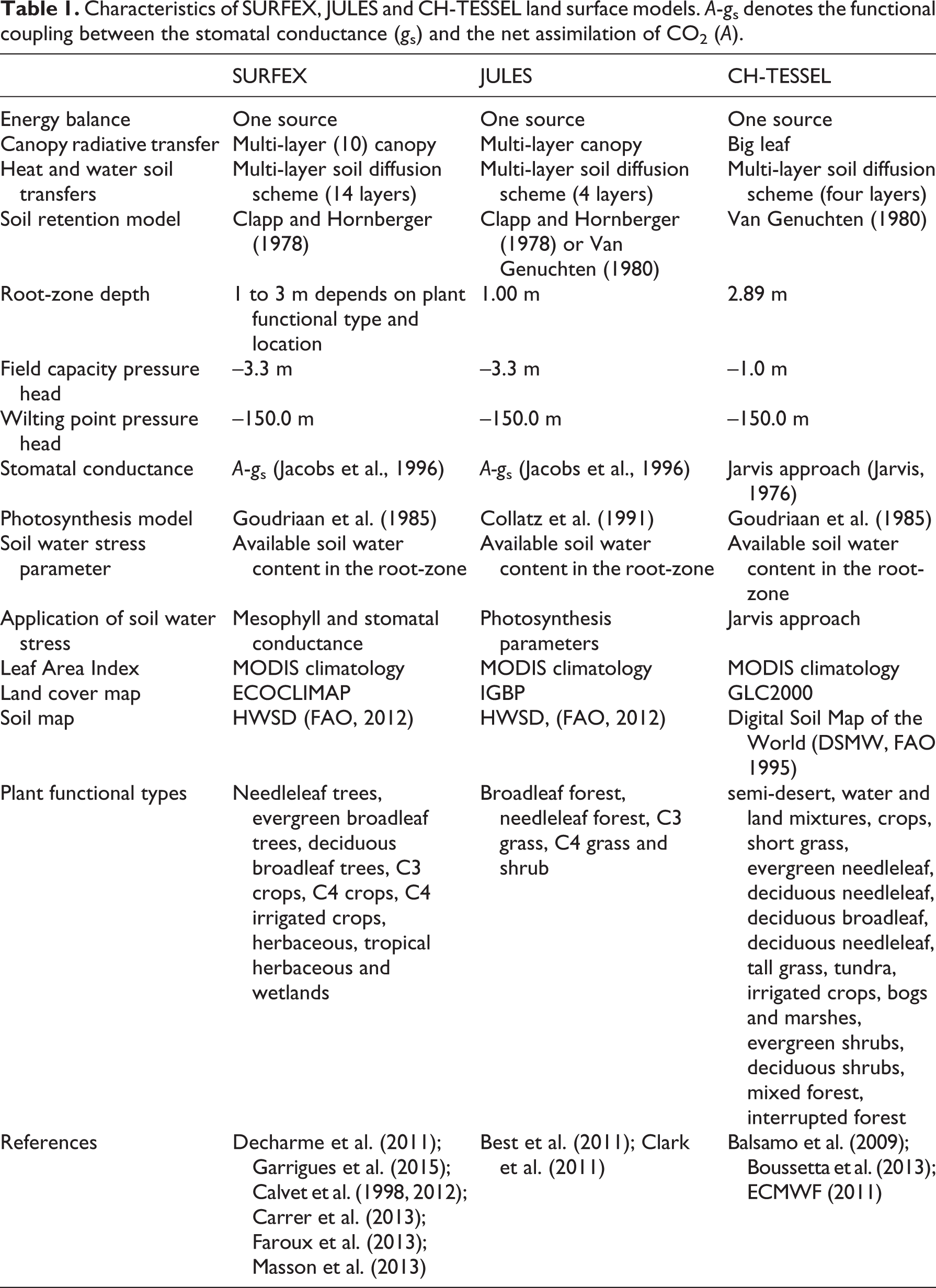
Table 1 provides the main characteristics of these models. These models are driven by a climatology of Leaf Area Index (LAI) and vegetation height. Their spatial integration is achieved using their default soil and vegetation ancillary data sets and land cover map. All models calculate a single source energy balance and use a multi-layer diffusion scheme to simulate water and heat transfer in the soil. While SURFEX and JULES represent the functional coupling between the stomatal conductance (g _s) and the net assimilation of carbon dioxide (CO₂) (photosynthesis, A), CHTESSEL relies on an empirical parametric formulation of the stomatal conductance.

Table 1.

Characteristics of SURFEX, JULES and CH-TESSEL land surface models. A-g _s denotes the functional coupling between the stomatal conductance (g _s) and the net assimilation of CO₂ (A).

	SURFEX	JULES	CH-TESSEL
Energy balance	One source	One source	One source
Canopy radiative transfer	Multi-layer (10) canopy	Multi-layer canopy	Big leaf
Heat and water soil transfers	Multi-layer soil diffusion scheme (14 layers)	Multi-layer soil diffusion scheme (4 layers)	Multi-layer soil diffusion scheme (four layers)
Soil retention model	Clapp and Hornberger (1978)	Clapp and Hornberger (1978) or Van Genuchten (1980)	Van Genuchten (1980)
Root-zone depth	1 to 3 m depends on plant functional type and location	1.00 m	2.89 m
Field capacity pressure head	–3.3 m	–3.3 m	–1.0 m
Wilting point pressure head	–150.0 m	–150.0 m	–150.0 m
Stomatal conductance	A-g _s (Jacobs et al., 1996)	A-g _s (Jacobs et al., 1996)	Jarvis approach (Jarvis, 1976)
Photosynthesis model	Goudriaan et al. (1985)	Collatz et al. (1991)	Goudriaan et al. (1985)
Soil water stress parameter	Available soil water content in the root-zone	Available soil water content in the root-zone	Available soil water content in the root-zone
Application of soil water stress	Mesophyll and stomatal conductance	Photosynthesis parameters	Jarvis approach
Leaf Area Index	MODIS climatology	MODIS climatology	MODIS climatology
Land cover map	ECOCLIMAP	IGBP	GLC2000
Soil map	HWSD (FAO, 2012)	HWSD, (FAO, 2012)	Digital Soil Map of the World (DSMW, FAO 1995)
Plant functional types	Needleleaf trees, evergreen broadleaf trees, deciduous broadleaf trees, C3 crops, C4 crops, C4 irrigated crops, herbaceous, tropical herbaceous and wetlands	Broadleaf forest, needleleaf forest, C3 grass, C4 grass and shrub	semi-desert, water and land mixtures, crops, short grass, evergreen needleleaf, deciduous needleleaf, deciduous broadleaf, deciduous needleleaf, tall grass, tundra, irrigated crops, bogs and marshes, evergreen shrubs, deciduous shrubs, mixed forest, interrupted forest
References	Decharme et al. (2011); Garrigues et al. (2015); Calvet et al. (1998, 2012); Carrer et al. (2013); Faroux et al. (2013); Masson et al. (2013)	Best et al. (2011); Clark et al. (2011)	Balsamo et al. (2009); Boussetta et al. (2013); ECMWF (2011)

2 Experiment design

The simulations were conducted from 1994 to 2012 over a 0.5° grid over Europe and at a three-hourly time step, using the WFDEI (WATCH Forcing Data methodology applied to ERA-Interim data; Weedon et al., 2014) atmospheric reanalysis. Two distinct simulations were conducted for JULES using distinct soil hydraulic parametrizations: one is based on the Van Genuchten (1980) scheme (JULES_VG) and one relies on the Clapp and Hornberger (1978) scheme (JULES_CH). We used the 1979–1993 period as a spin-up period and the model’s outputs were analyzed from 1994 to 2012.

The spatial patterns of the model outputs were evaluated over three European geographic domains – namely, the UK, France and Spain – which were selected to represent contrasting climate, soil and vegetation characteristics (Table 2). The variogram analysis is applied to the latent heat (LE), sensible heat (H), net radiation (RN) fluxes and the root-zone liquid soil moisture content (θ) variables. Three-hourly model outputs are first averaged over 10 days. Next, the 10-day values are averaged over the entire simulation period (1994–2012) to represent a mean climatological annual timeseries – that is, 36 10-day values. The variograms of the mean climatological values of each flux and variable are then computed.

Table 2.

Geographic domains.

Domain	ULC latitude	ULC longitude	LRC latitude	LRC longitude
France	50.25	–2.25	43.75	5.75
Spain	43.25	–9.25	36.25	2.25
UK	58.75	–9.25	50.75	1.75

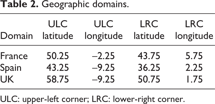
ULC: upper-left corner; LRC: lower-right corner.

III Geostatistical methodology to quantify the spatial patterns of model outputs

The variogram analysis consists of two steps: i) computing the empirical variogram over the domain of interest; and ii) fitting a theoretical variogram model to the empirical variogram to retrieve the spatial variability and the size of the spatial structures of the data.

1 Empirical variogram

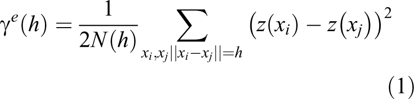
The empirical variogram γ^e (h) (equation (1)) measures the dissimilarity between the model outputs z(x_i ) and z(x_j ) taken at two distinct grid cells, x_i and x_j , separated by a distance, h (equation (1)). To provide statistically meaningful variogram values, the pairs of grid cells at a similar distance, h, are grouped into bins of separation distance. N(h) is the number of grid cell pairs within each bin. The variogram is computed as the average of the squared differences of the model values (z(x_i ) and z(x_j )) of all pairs of grid cells that fall within each distance bin. To properly sample the range of separation distance, h, between grid cells, the bin size is set to one grid cell. The variogram is computed to a maximum distance equal to half the domain size to ensure that there are enough grid cell pairs within in each distance bin (Garrigues et al., 2006).

γ^{e} (h) = \frac{1}{2 N (h)} \sum_{x_{i}, x_{j} ‖ x_{i} - x_{j} ‖ = h} {(z (x_{i}) - z (x_{j}))}^{2}

2 Variogram modelling

We assume that the model outputs (z(x_i ) and z(x_j )) are realizations of a random function Z(x). Under the second-order stationarity hypothesis (Chiles and Delfiner, 2012), which ensures the existence and the stationarity of the first and second moments of Z(x), the theoretical variogram, γ(h), is defined by:

γ (h) = 0.5 V a r [Z (x + h) - Z (x)] = σ^{2} - C (h)

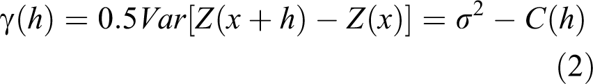
where C(h) and σ ² are the covariance and the variance of Z(x), respectively. γ(h) is a function starting from 0 for h = 0 and converging to the sill, σ ², as h tends to infinity. The range, r, of the theoretical variogram is the distance at which it reaches the sill. Data separated by a distance larger than the range are spatially uncorrelated.

The linear model of regionalization, which models the variogram as a linear combination of elementary conditionally definite negative functions g_k (h), is defined by:

γ (h) = σ^{2} \sum_{i = 1}^{k} (b_{k} g_{k} (h))

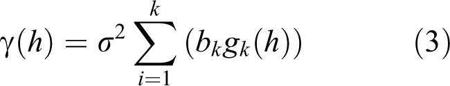
where b_k is the weight associated to each function, g_k (h). In an exploratory approach, distinct combinations of distinct g_k functions (spherical, exponential, Gaussian) were tested and it was found that a single exponential model was providing the best fit to our data.

Equation (3) then becomes:

γ (h) = σ^{2} [1 - e x p (\frac{- 3 h}{r})]

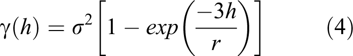
The parameters σ ² and r of the exponential variogram model are estimated by least-square fitting to the experimental variogram.

The integral range derived from the variogram (A, equation (5)) is used to quantify the spatial structures of the data. A is an area moment that represents the mean surface of the spatial structure of the variable over a given spatial domain (Chiles and Delfiner, 2012).

A = \frac{1}{σ^{2}} \int_{h \in ℝ^{2}} (σ^{2} - γ (h))

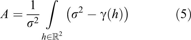
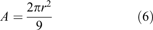
The value of A for an exponential variogram model can be analytically derived from equation (4) and is directly proportional to the variogram range:

A = \frac{2 π r^{2}}{9}

3 Variogram modelling assumptions

The modelling of the variogram relies on the second-order stationarity hypothesis, which implies that the data do not exhibit any spatial trend within the geographic domain and allows to use the variogram range to quantify the length scale of the data. As demonstrated by Garrigues et al. (2006), the integral range can be used as an a posteriori yardstick to judge if the size of the geographic domain is large enough to measure properly the length scale of the data with the variogram. We verified that the integral range of most of the modelled variograms are small enough compared to the surface of the geographic domain that justifies the validity of the second-order stationarity hypothesis.

We chose to not include any nugget component (discontinuity at the origin) to represent unresolved sub-grid variability. We checked that including a nugget term in equation (3) did not improve the quality of the variogram fit and does not change the estimation of the length scale of the data. This work is focused on the characterization of large-scale spatial structures and the characterization of sub-grid heterogeneity, which would require data at a finer spatial resolution, is beyond the scope of this work.

4 Spatial pattern analysis

The spatial patterns of the variables of interest are characterized by the square root of the variogram sill (i.e. $σ$ ), which quantifies the degree of spatial variability of the data, and by the variogram integral range (A), which quantifies the mean surface of the spatial structures (i.e. patches) displayed by the data. The unit of $σ$ is that of the variable (W m^–2 for the surface fluxes and m³ m^–3 for soil moisture). The unit of A is that of the surface of a grid cell (0.25 deg²).

The analysis involves quantifying the seasonal evolution of A and $σ$ , and assessing the differences across geographic domains, variables and models. We use the root-mean-square difference (RMSD) to quantify the differences in A and $σ$ between model experiments.

Variograms were also computed for two key surface properties:

the maximum water content available for the plant transpiration (MaxAWC), which is defined as the difference between the soil moisture at field capacity and the soil moisture at wilting point; this is a key driver of ET dynamics (Garrigues et al., 2015). MaxAWC is constant in time, so one variogram is computed for each model and each geographic domain.

the monthly LAI, which represents the vegetation seasonal cycle. For each LSM, a variogram of LAI was computed over each geographic domain at a monthly time step. In this report, we showed the results for France to illustrate the relationship between the spatial patterns of LAI and that of surface fluxes.

IV Drivers of the spatial patterns of surface fluxes and soil moisture

1 Impact of climate

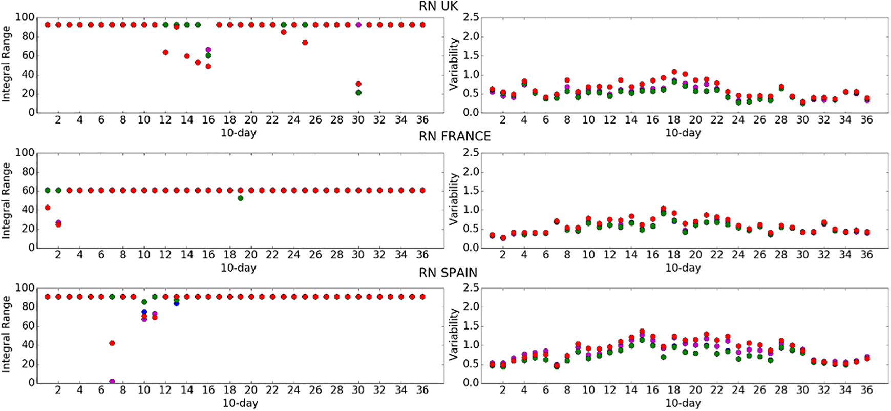
Figure 1 shows that the seasonal variations of A and $σ$ of net radiation are low compared to those calculated for latent and sensible heat fluxes. Net radiation is strongly driven by the climate and its spatial pattern does not have a strong seasonal signal.

Figure 1.

Temporal evolution of the integral range (A) and the spatial variability (σ) of RN at 10-day time steps over the UK, France and Spain, for SURFEX (magenta), JULES_VG (blue), JULES_CH (green) and CHTESSEL (red) experiments. For interpretation of the references to colours in this figure legend, refer to the online version of this article.

2 Impact of surface characteristics

The lower values of A generally obtained over France indicate a smaller size of spatial structures compared to the UK and Spain. This is related to the smaller spatial structures observed for the soil hydraulic properties (Figure 2) and for LAI (Figure 3) over France.

Figure 2.

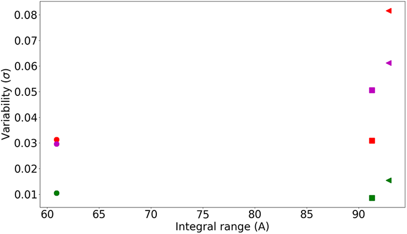
Comparison of the integral range (A) and the spatial variability (σ) of the maximum available water content (MaxAWC) across models and geographic domains. Models are represented by distinct colors: SURFEX in magenta, JULES_VG in blue, JULES_CH in green and CHTESSEL in red. Geographic domains are represented by distinct symbols: UK (triangle), France (circle), Spain (square). For interpretation of the references to colours in this figure legend, refer to the online version of this article.

Figure 3.

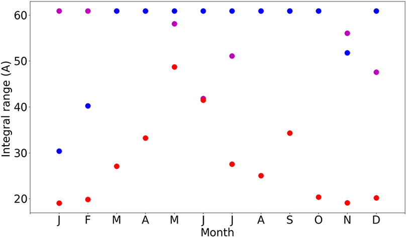
Seasonal evolution of the integral range (A) of LAI over France, for SURFEX (magenta), JULES_VG (blue) and CHTESSEL (red) models. For interpretation of the references to colours in this figure legend, refer to the online version of this article.

3 Impact of vegetation dynamics

The spatial variability of sensible and latent heat fluxes exhibits strong seasonal variations and is the highest in late spring and early summer (Figures 4 and 5). This is related to the development of vegetation in spring and summer, which results in a higher spatial variability of LAI as shown by Figure 6. The contrast between the response of vegetated and non-vegetated surface to the climate forcing is more important in summer, which increases the spatial variability of surface fluxes. Also, evapotranspiration is more frequently limited by soil moisture during spring and summer; this contributes to the larger spatial variability in latent heat fluxes.

Figure 4.

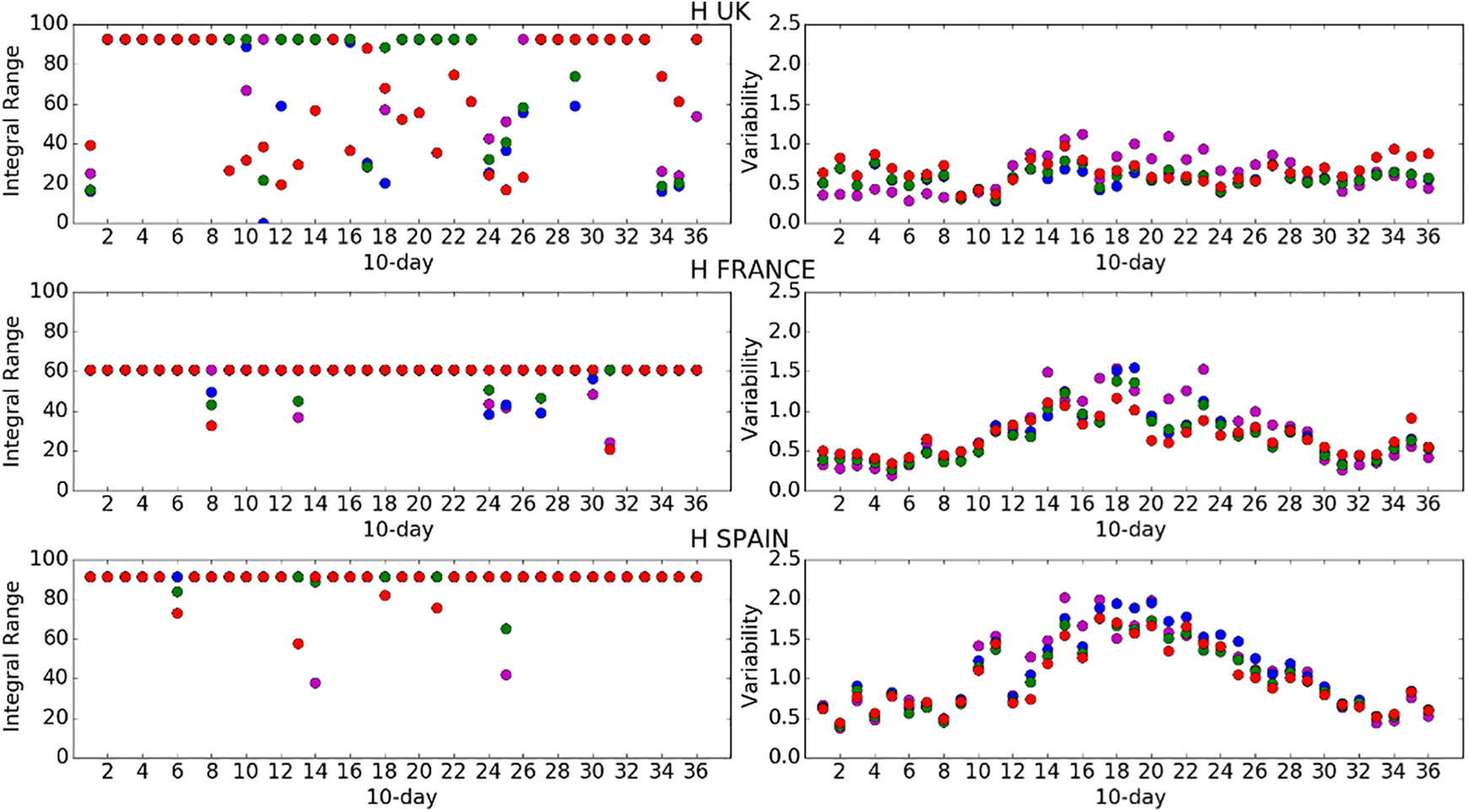
Temporal evolution of the integral range (A) and the spatial variability (σ) of H at 10-day time steps over the UK, France and Spain, for SURFEX (magenta), JULES_VG (blue), JULES_CH (green) and CHTESSEL (red) experiments. For interpretation of the references to colours in this figure legend, refer to the online version of this article.

Figure 5.

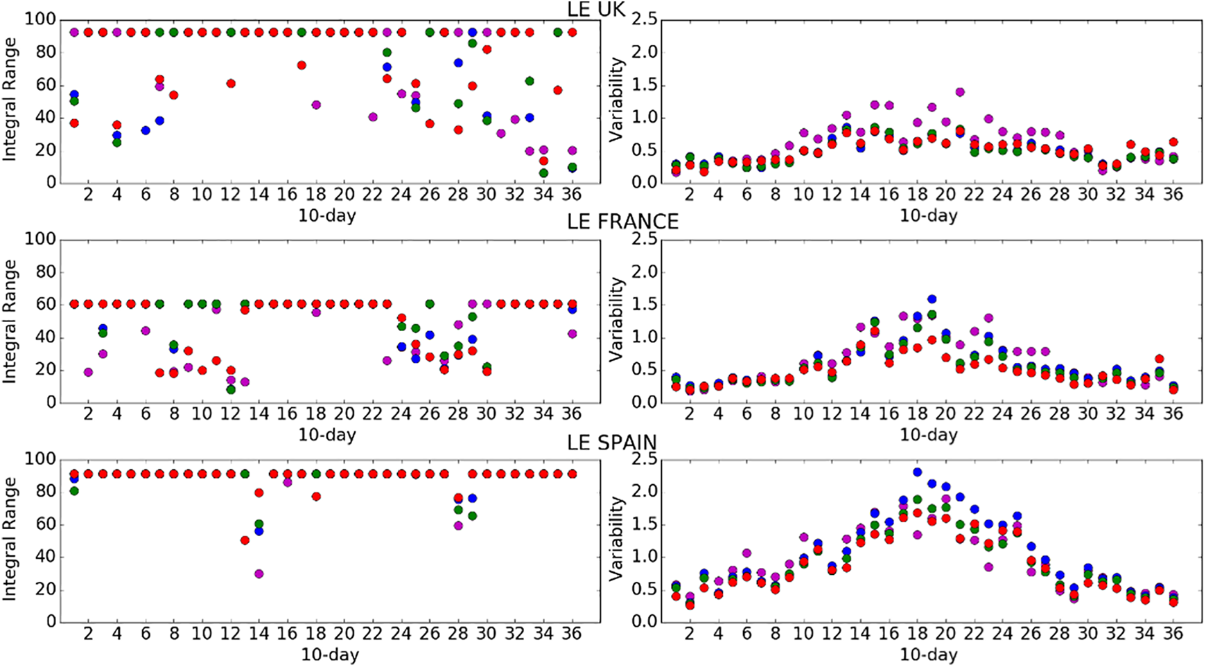
Temporal evolution of the integral range (A) and the spatial variability (σ) of LE at 10-day time steps over the UK, France and Spain, for SURFEX (magenta), JULES_VG (blue), JULES_CH (green) and CHTESSEL (red) experiments. For interpretation of the references to colours in this figure legend, refer to the online version of this article.

Figure 6.

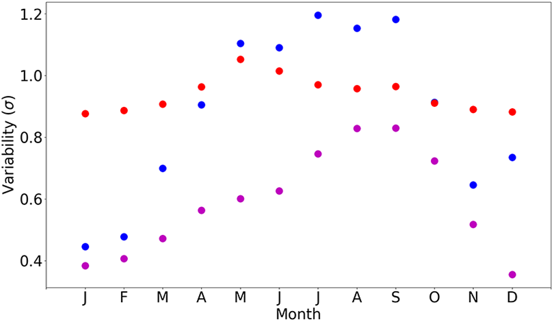
Seasonal evolution of the spatial variability (σ) of LAI over France, for SURFEX (magenta), JULES_VG (blue) and CHTESSEL (red) models. For interpretation of the references to colours in this figure legend, refer to the online version of this article.

4 Impact of soil moisture stress

The larger seasonal variations of $σ$ for sensible and latent heat fluxes observed over France and Spain compared to the UK (Figures 4 and 5) is most likely related to a more frequent occurrence of the soil-moisture-limited regime in the south of France and in Spain. Soil moisture stress generates large spatial contrasts in the energy partitioning between latent and sensible heat, which explains the increase of the spatial variability of surface fluxes during dry spells.

V Drivers of the differences in spatial patterns between models

Tables 3 and 4 indicate that the differences in A and $σ$ are lower for the comparison between SURFEX and JULES compared to the comparison of these models with CHTESSEL, which has the highest RMSD. The largest discrepancies between models are obtained for sensible and latent heat fluxes and root-zone soil moisture. We investigate below the main drivers of these discrepancies.

Table 3.

RMSD in integral range (A) of 10-day mean values of RN, H, LE and root-zone soil moisture between SURFEX, JULES_CH, JULES_VG and CHTESSEL.

Experiments	RN			H			LE			Soil moisture
Model_x vs Model_y	UK	FR	SP	UK	FR	SP	UK	FR	SP	UK	FR	SP
SURFEX vs JULES_VG	11.91	5.66	15.23	21.33	8.53	12.09	27.20	17.12	5.79	8.92	20.87	11.30
SURFEX vs JULES_CH	11.98	5.82	15.43	16.78	8.34	9.40	27.72	16.66	7.14	22.10	15.72	11.78
SURFEX vs CHTESSEL	15.01	3.01	6.72	35.61	7.80	14.00	34.54	20.68	11.38	5.12	20.24	11.30
JULES_VG vs JULES_CH	0.12	1.35	1.76	13.58	4.78	4.56	14.80	5.72	2.52	17.67	19.81	4.63
JULES_VG vs CHTESSEL	10.72	6.74	9.04	33.60	9.41	7.06	27.04	13.67	8.57	10.28	26.34	0.00
JULES_CH vs CHTESSEL	10.75	6.87	9.28	33.95	7.95	7.93	23.31	14.93	9.20	20.75	23.31	4.63
Mean values	10.08	4.90	9.58	25.81	7.80	9.17	25.77	14.80	7.43	14.14	21.05	7.27

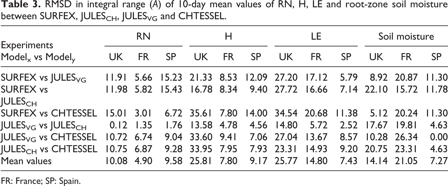
FR: France; SP: Spain.

Table 4.

RMSD of spatial variability (σ) of 10-day RN, H, LE and root-zone soil moisture between SURFEX, JULES_CH, JULES_VG and CHTESSEL.

Experiments	RN			H			LE			Soil moisture
Model_x vs Model_y	UK	FR	SP	UK	FR	SP	UK	FR	SP	UK	FR	SP
SURFEX vs JULES_VG	0.06	0.03	0.14	0.23	0.21	0.14	0.24	0.17	0.29	1.83	2.65	5.65
SURFEX vs JULES_CH	0.06	0.03	0.15	0.21	0.21	0.15	0.24	0.17	0.18	3.21	0.44	0.36
SURFEX vs CHTESSEL	0.13	0.09	0.09	0.26	0.25	0.19	0.24	0.25	0.21	7.28	2.10	4.63
JULES_VG vs JULES_CH	0.01	0.01	0.01	0.04	0.05	0.13	0.03	0.07	0.19	1.72	2.89	5.54
JULES_VG vs CHTESSEL	0.17	0.10	0.21	0.15	0.16	0.17	0.08	0.19	0.25	8.75	0.67	1.05
JULES_CH vs CHTESSEL	0.17	0.10	0.21	0.13	0.13	0.08	0.08	0.13	0.10	10.38	2.33	4.52
Mean	0.1	0.06	0.135	0.17	0.17	0.14	0.15	0.16	0.20	5.53	1.85	3.63

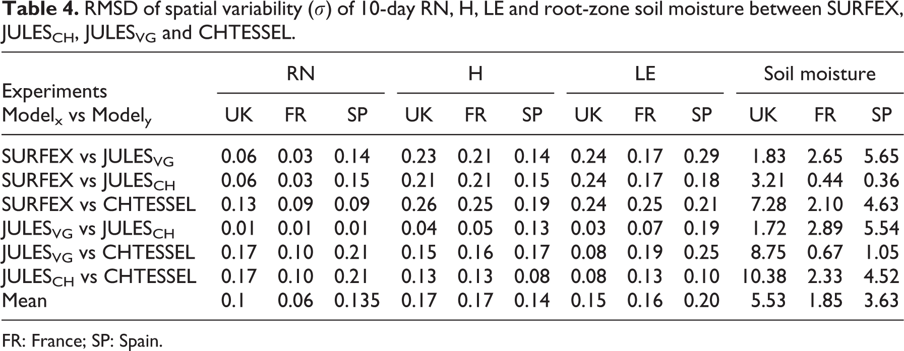
FR: France; SP: Spain.

1 Impact of forcing data set

Figure 1 shows small differences in A and $σ$ of net radiation across models. This is supported by the higher RMSD of spatial variability between models, for H and LE, compared to those calculated for RN (Table 4). The main explanation is that the climate forcing data set, which contains the main drivers of net radiation – that is, shortwave and longwave incoming radiation – is identical across experiments. Conversely, latent and sensible heat fluxes exhibit larger differences in spatial patterns between experiments, which arise from the differences in i) the soil and vegetation data sets implemented in each model and ii) physical process representation such as stomatal conductance parametrization.

2 Impact of soil hydraulic parametrization

The largest differences in $σ$ between models are observed for the root-zone soil moisture. For France and Spain, we identified two combinations of models with similar $σ$ values (Figure 7 and Table 4):

JULES_VG and CHTESSEL with the highest $σ$ values;

JULES_CH and SURFEX with the lowest $σ$ values.

Figure 7.

Temporal evolution of the integral range (A) and the spatial variability (σ) of the root-zone soil moisture at 10-day time steps over the UK, France and Spain, for SURFEX (magenta), JULES_VG (blue), JULES_CH (green) and CHTESSEL (red) experiments. For interpretation of the references to colours in this figure legend, refer to the online version of this article.

Conversely for the UK, JULES_CH, JULES_VG and SURFEX provide similar $σ$ values of soil moisture, while CHTESSEL shows much higher values than the rest of the models.

The simulation of surface fluxes is hugely dependent on the soil hydraulic parametrization and soil property map (Garrigues et al., 2015), which can exhibit different spatial patterns across models. SURFEX and JULES_CH are based on the Clapp and Hornberger (1978) model, while JULES_VG and CHTESSEL rely on the Van Genuchten (1980) model. This observation holds over France and Spain; this suggests that the impact of the type of soil hydraulic parametrization on the surface flux spatial patterns is stronger than the type of soil map used to infer the soil properties over these domains. Conversely, over the UK, the substantial differences in spatial variability between CHTESSEL and the rest of the model experiments are probably related to differences in the spatial distribution of soil properties. This is confirmed by the variograms computed on the soil hydraulic properties (MaxAWC; Figure 2), which exhibit large discrepancies in the spatial variability of MaxAWC between models over the UK.

3 Impact of LAI

The LAI value of each grid cell is the result of the LAI data set and the land cover map implemented in each model. While the models rely on the same satellite LAI data set, they use different land cover classifications (see Table 1), which may generate distinct spatial distributions of grid cell LAI values. This is illustrated over France where the models exhibit large discrepancies in both the LAI spatial structures (Figure 3) and the time course of the LAI spatial variability (Figure 6). Figure 6 shows that, over France, SURFEX and JULES display more pronounced seasonal variations of LAI spatial variability than CHTESSEL, which is concurrently observed for the latent heat flux in Figure 5. JULES shows the highest values of LAI spatial variability during the summer, which concurrently results in the highest spatial variability of latent heat flux during the summer. The shift in the seasonal variation of LAI spatial variability of SURFEX and JULES observed over France (Figure 6) is also observed for the latent heat flux (Figure 5). These examples clearly show that the LAI spatial variability is a key driver of the spatial variability of the simulated surface fluxes.

VI Conclusions

This work shows that variogram modeling is a powerful tool to quantify the differences in LSM outputs through two components:

the degree of spatial variability quantified by the variogram sill; and

the surface of the spatial structure of the data represented by the variogram integral range.

Variogram analysis was applied to surface fluxes and soil moisture simulated by three LSMs over three European domains with contrasted climates (UK, France and Spain).

The main outcomes are as follows:

The models show larger differences in the spatial variabilities of the turbulent heat fluxes, which are more prominently driven by i) soil and vegetation ancillary data and ii) physical process representation, compared to the net radiation spatial variability, which is mainly driven by the radiative climate forcing.

The seasonal evolution of the spatial variability of LAI and that of latent heat flux show large similarities. The increase in spatial variability of sensible and latent heat fluxes in spring and summer is related to the enhancement of the spatial variability of LAI, which creates a larger spatial contrast in the surface response to the climate forcing. The higher seasonal variations of spatial variability in turbulent heat fluxes observed over France and Spain are most likely related to a more frequent occurrence of soil-moisture-limited ET regime during summer dry spells in Spain and the south of France.

The highest discrepancies in spatial patterns between models are observed for soil moisture. Over France and Spain, the spatial patterns of soil moisture are primarily related to by the type of soil hydraulic function (Van Genuchten (1980) vs Clapp and Hornberger (1978)), while over the UK, the differences between models are related mainly to differences in soil maps that determine the parameters of the soil hydraulic functions.

This report highlights the capability of the variogram to measure the spatial patterns of LSM outputs, to monitor the seasonal changes in spatial patterns and to quantify the differences in spatial patterns across variables, geographic domains and models. The integral range is a powerful metric to verify if the model simulations resolve similar spatial features. The variogram sill allows the detection of differences in the spatial variability across models that can be related to differences in the spatial distribution of the surface parameters used by each model. Therefore, we strongly encourage the implementation of the variogram metrics in model intercomparison exercises to enhance our understanding of the spatiotemporal structure of the uncertainties associated with LSMs. In addition, the variogram analysis proposed in this work can be applied to satellite observations of surface fluxes and surface characteristics to evaluate the accuracy of the spatial patterns of surface fluxes simulated by LSMs.

A key assumption of the variogram modelling approach used in this work is the second-order stationarity, which implies that the data do not exhibit any spatial trend and allows us to use the variogram to quantify the length scale of the data. The integral range, which represents the average surface of the data spatial structure, can be used to verify, a posteriori, the validity of this assumption. The size of the geographic domain should be adjusted to have an integral range much smaller than the surface of the geographic domain used to compute the variogram. Besides, in this work, we chose to model the variogram using a single exponential model to demonstrate the capability of the variogram metrics to characterize the model output’s spatial patterns. A first improvement could be to include additional elementary functions in the linear model of regionalization (equation (2)) to describe multiple length scales in the data. While this can be relevant for small spatial domains, we did not find any improvements for the large domains investigated in this work. Another possible avenue for improvement is to use alternative types of covariance models. Genton and Kleiber (2015) demonstrate the flexibility of the Matern covariance function to describe correlation at both large (scale parameter) and small distances (smoothness parameter). In addition, in this work, we modeled the spatial patterns for each 10-day time step and then we observed the temporal evolution of the variogram metrics. An alternative approach could be to implement a space–time version of the linear model of regionalization to describe the spatiotemporal structure of the model outputs (De Iaco et al., 2013). Variograms can be modelled within a multivariate framework to investigate the co-variability between variables. This could be applied in further research to analyze the spatial dynamics of ET–soil moisture relationships, and to identify the discrepancies in the representation of the spatial dynamics of drought across models.

Footnotes

Declaration of conflicting interests

The author(s) declared no potential conflicts of interest with respect to the research, authorship, and/or publication of this article.

Funding

The author(s) received no financial support for the research, authorship, and/or publication of this article.

ORCID iD

S Garrigues

EL Robinson

References

Balsamo

Viterbo

ACM

Beljaars

BJJM

, et al. (2009) A revised hydrology for the ECMWF model: Verification from field site to terrestrial water storage and impact in the ECMWF-IFS. Journal of Hydrometeorology 10: 623–643.

Best

Pryor

Clark

, et al. (2011) The Joint UK Land Environment Simulator (JULES), model description. Part 1: Energy and water fluxes. Geoscientific Model Development Discussions 4: 595–640.

Best

Abramowitz

Johnson

, et al. (2015) The plumbing of land surface models: Benchmarking model performance. Journal of Hydrometeorology 16: 1425–1442.

Boone

de Rosnay

Basalmo

, et al. (2009) The AMMA land surface model intercomparison project. Bulletin of the American Meteorological Society 90: 1865–1880. DOI: 10.1175/2009BAMS2786.1.

Boussetta

Balsamo

Beljaars

, et al. (2013) Natural land carbon dioxide exchanges in the ECMWF Integrated Forecasting System: Implementation and offline validation. Journal of Geophysical Research 118: 5923–5946.

Calvet

J-C

Noilhan

Roujean

J-L

, et al. (1998) An interactive vegetation SVAT model tested against data from six contrasting sites. Agricultural and Forest Meteorology 92: 73–95.

Calvet

J-C

Lafont

Cloppet

, et al. (2012) Use of agricultural statistics to verify the interannual variability in land surface models: A case study over France with ISBA-A-gs. Geoscientific Model Development 5: 37–54.

Carrer

Roujean

J-L

Lafont

, et al. (2013) A canopy radiative transfer scheme with explicit FAPAR for the interactive vegetation model ISBA-A-gs: Impact on carbon fluxes. Journal of Geophysical Research: Biogeosciences 118: 888–903.

Chiles

Delfiner

(2012) Geostatistics: Modeling Spatial Uncertainty. 2nd ed. New York: Wiley.

10.

Clapp

Hornberger

(1978) Empirical equations for some soil hydraulic properties. Water Resources Research 14: 601–604.

11.

Collatz

Ball

Grivet

Berry

(1991) Physiological and environmentalregulation of stomatal conductance, photosynthesis and transpiration -a model that includes laminar boundary layer. Agricultural and Forest Meteorology 54: 107–136.

12.

Csillag

Kabos

(2002) Wavelets, boundaries and the analysis of landscape pattern. Ecoscience 9: 177–190.

13.

Decharme

Boone

Delire

, et al. (2011) Local evaluation of the interaction between Soil Biosphere Atmosphere soil multilayer diffusion scheme using four pedotransfer functions. Journal of Geophysical Research 116: D20126.

14.

De Iaco

Myers

Palma

, et al. (2013) Using simultaneous diagonalization to identify a space–time linear coregionalization model. Mathematical Geosciences 45: 69–86.

15.

Dirmeyer

(2011) A history and review of the Global Soil Wetness Project (GSWP). Journal of Hydrometeorology 12: 729–749.

16.

ECMWF (2011) IFS documentation Cy37r2. Part IV: Physical processes, Chapter 8. Available at: https://www.ecmwf.int/en/elibrary/9239-part-iv-physical-processes (accessed January 2021).

17.

Eyring

Righi

Lauer

, et al. (2016) ESMValTool (v1.0)—A community diagnostic and performance metrics tool for routine evaluation of Earth system models in CMIP. Geoscientific Model Development 9(5): 1747–1802.

18.

FAO (1995) Digital Soil Map of the World and derived properties (ver. 3.5). FAO Land and Water Digital Media Series # 1. FAO: Rome.

19.

FAO, IIASA, ISRIC, ISSCAS, JRC (2012) Harmonized World Soil Database (version 1.2). FAO, Rome, Italy and IIASA, Laxenburg, Austria. p. 42.

20.

Faroux

Kaptué Tchuenté

Roujean

J-L

, et al. (2013) Ecoclimap-II/Europe: A twofold database of ecosystems and surface parameters at 1 km resolution based on satellite information for use in land surface, meteorological and climate models. Geoscientific Model Development 6: 563–582.

21.

Garrigues

Allard

Baret

, et al. (2006) Quantifying spatial heterogeneity at the landscape scale using variogram models. Remote Sensing of Environment 103: 81−96.

22.

Garrigues

Allard

Baret

(2007) Using first- and second-order variograms for characterizing landscape spatial structures from remote sensing imagery. IEEE Transactions on Geoscience and Remote Sensing 45(6): 1823–1834.

23.

Garrigues

Allard

Baret

(2008) Modeling temporal changes in surface spatial heterogeneity over an agricultural site. Remote Sensing of Environment 112(2): 588–602.

24.

Garrigues

Olioso

Carrer

, et al. (2015) Impact of climate, vegetation, soil and crop management variables on multi-year ISBA-A-gs simulations of evapotranspiration over a Mediterranean crop site. Geoscientific Model Development 8: 3033–3053.

25.

Genton

Kleiber

(2015) Cross-covariance functions for multivariate geostatistics. Statistical Science 30: 147–163.

26.

Goudriaan

van Laar

van Keulen

, et al. (1985) Photosynthesis, CO₂ and plant production. In: W

Day

Atkin

(eds) Wheat Growth and Modelling. NATO ASI Series, Series A, 86. New York: Plenum Press, 107–122.

27.

Harris

Folwell

Gallego-Elvira

, et al. (2017) An evaluation of modeled evaporation regimes in Europe using observed dry spell land surface temperature. Journal of Hydrometeorology 18: 1453–1470.

28.

Henderson-Sellers

Yang

Z-L

Dickinson

(1993) The project for intercomparison of land-surface parameterization schemes. Bulletin of the American Meteorological Society 74(7): 1335–1349.

29.

Jacobs

Van den Hurk

De Bruin

(1996) Stomatal behaviour and photosynthetic rate of unstressed grapevines in semi-arid conditions. Agricultural and Forest Meteorology 80(2-4): 111–134.

30.

Jarvis

(1976) The interpretation in the variations of leaf water potential and stomatal conductance found in canopies in the field. Philosophical Transactions of the Royal Society B 273: 593–610.

31.

Julesz

(1962) Visual pattern discrimination. Institute of Radio Engineers Transactions on Information Theory 8: 84–92.

32.

Koster

Sud

Guo

, et al. (2006) GLACE: The Global Land-Atmosphere Coupling Experiment. Part I: Overview. Journal of Hydrometeorology 7(4): 590–610.

33.

Kumar

Peters-Lidard

Santanello

, et al. (2012) Land surface Verification Toolkit (LVT) – a generalized framework for land surface model evaluation. Geoscientific Model Development 5: 869–886.

34.

Luo

Randerson

Abramowitz

, et al. (2012) A framework for benchmarking land models. Biogeosciences 9(10): 3857–3874.

35.

Masson

Le Moigne

Martin

, et al. (2013) The SURFEXv7.2 land and ocean surface platform for coupled or offline simulation of earth surface variables and fluxes. Geoscientific Model Development 6: 929–960.

36.

Noilhan

Planton

(1989) A simple parameterization of land surface processes for meteorological models. Monthly Weather Review 117: 536–549.

37.

Pontius

Malanson

(2005) Comparison of the structure and accuracy of two land change models. International Journal of Geographical Information Science 19(2): 243–265.

38.

Pontius

Thontteh

Chen

(2008) Components of information for multiple resolution comparison between maps that share a real variable. Environmental and Ecological Statistics 15: 111–142.

39.

Seneviratne

Corti

Davin

, et al. (2010) Investigating soil moisture–climate interactions in a changing climate: A review. Earth Science Reviews 99: 125–161.

40.

Tarnavsky

Garrigues

Brown

(2008) Multiscale geostatistical analysis of AVHRR, SPOT-VGT, and MODIS NDVI products. Remote Sensing of Environment 112(2): 535–549.

41.

Ukkola

De Kauwe

Pitman

, et al. (2016) Land surface models systematically overestimate the intensity, duration and magnitude of seasonal scale evaporative droughts. Environmental Research Letters 11: 104012.

42.

Van Genuchten

(1980) A closed-form equation for predicting the hydraulic conductivity of unsaturated soils. Soil Science Society of America Journal 44: 892–898.

43.

Vilasa

Miralles

de Jeu

RAM

, et al. (2017) Global soil moisture bimodality in satellite observations and climate models. Journal of Geophysical Research: Atmospheres 122: 4299–4311.

44.

Weedon

Balsamo

Bellouin

, et al. (2014) The WFDEI meteorological forcing data set: WATCH Forcing Data methodology applied to ERA-Interim reanalysis data. Water Resources Research 50: 7505–7514.