Wind resource assessment of Cuba in future climate scenarios

Abstract

The future climatic behavior of the wind resource in Cuba has not been studied in the past. This study presents a preliminary analysis of the behavior of wind speed using the regional climate model PRECIS (Providing Regional Climates for Impacts Studies) in high-resolution scenarios of climate change SRES A1B (Special Report on Emissions Scenarios), driven with boundary conditions from the General Circulation Model ECHAM5 (European Centre/HAMburg climate model) and 6 of the 16 members of the set of perturbed physics HadCM3 (Hadley Center Coupled Model, version 3) global climate model. Changes in the distribution of wind speed for three periods of 30 years in the future—2011–2040, 2041–2070, and 2071–2099—are analyzed. The PRECIS model was also run with reanalysis data during the period of 1 January 1989 to 31 December 2002. It was found that changes in wind speed will be larger in the eastern and northern coast, becoming statistically significant for the second half of this century with an increase in wind magnitude between 0.1 and 0.4 m s⁻¹. These areas of increased wind power match with the current projection of the Cuban wind program where the construction of 13 new wind farms are contemplated. Finally, this increase is added to the wind speed outputs of the numerical wind atlas of Cuba to estimate the values of wind speed over the three future periods.

Keywords

Wind resource assessment climate model PRECIS changes wind speed wind power numerical wind atlas of Cuba

Introduction

Exploring the impact of climate change on wind energy is a focus of research and scientific analysis in many countries around the world. Several studies have shown that the wind has changed over the planet during the past three decades as indicated by measurements in the boundary layer and in the surface layer of the atmosphere.

For some regions of Europe, Pryor et al. (2012b) and Barstad et al. (2012) investigated the interannual variability of wind power potential, considering dynamic statistical scale reduction approaches under future climatic conditions (focusing on the British Isles, North Sea, Scandinavia, and the Baltic Sea). The great majority of these studies agree on an increase in average wind speed, especially in winter. Pryor et al. (2012a) investigated the interannual variability of the wind potential for future climate using HadCM3 (Hadley Center Coupled Model, version 3) model and found no substantial change in interannual wind variability. Pryor et al. (2012a) pointed out that a possible critical factor for such results is the resolution of the model, which also has a strong impact on wind climatology, which may be even of the same order of magnitude as the climate change.

Another study was done by Yao et al. (2012) in which a high-resolution regional climate model (RCM; Providing Regional Climates for Impacts Studies (PRECIS)) is used as a method to reduce the dynamic scale of future wind speed over Ontario. Changes in wind potential density and energy production were investigated through case studies. The spatial patterns and the magnitude of the wind speed from the PRECIS model outputs were in agreement with the Canadian Wind Atlas (Yu et al., 2006) and observations dataset. Their results indicated that there is likely going to be a decrease of up to 5% in wind speed over southern Ontario from the present to the period 2071–2100. Case studies of Yao et al. (2012) showed that changes in wind energy production are not proportional to changes in mean wind speed due to variations in wind speed distribution, so it would be reasonable to develop the wind energy industry around the Bay of Georgia and James Bayen either onshore or offshore, taking into account the increase in wind speed in these areas. Romanic et al. (2017) presented a methodology for microscale numerical modeling of urban wind resource assessment in changing climate. The methodology is applied for a specific urban development in the city of Toronto, Canada.

Also, Hueging et al. (2013) investigated the impact of climate change on the generation of wind energy in Europe, performing an ensemble of two RCMs and feeding them with a global climate model (GCM). The power density and its interannual variability are calculated on the basis of the wind speeds on the surface. They used several RCMs to simulate the behavior and variability of the wind potential. Saarnak et al. (2014) studied the uncertainties in the length of the seasonal measurements. With a series of 29 years, they used different methods of MCP (measure-correlate-predict) and several reanalysis data. Soldatenko and Karlin (2014) analyzed the effects of global climate change on the patterns of the general circulation of the atmosphere, the large-scale temperature field, as well as the wind velocity in the planetary boundary layer, and Vautard et al. (2014) simulated future climate impacts on electric power production.

In a more recent study, Balog et al. (2016) performed numerical simulations of near-surface wind fields from RCMs in order to obtain and fill the gaps in observations over the Mediterranean basin. Also, they presented the wind energy potential atlas and the map of a wind turbine’s functional range over this region. On the contrary, Da Silva et al. (2017) applied a dynamic downscaling technique on the Regional Atmospheric Modeling System (RAMS6.0) forced by output fields of the global circulation model HadGEM2-ES to estimate the wind potential over the regions of Mozambique considering the climate change scenario defined by Intergovernmental Panel on Climate Change (IPCC). At the end of the same year, Matthew and Ohunakin (2017) determined the effects of global warming and future afforestation on wind power potential in Nigeria using series of multi-year simulations of an RCM (ICTP-RegCM3) for the periods 1981–2000 (baseline) and 2031–2050 (future with elevated CO₂ under A1B emission scenario).

Compared to other regions of the world, the use of RCMs in the Caribbean region is relatively limited, although in recent years there has been a noticeable increase in the use of these tools. According to the reviewed literature, one of the first studies was produced by Angeles et al. (2007). They integrated the regional model RAMS coupled with the PCM (polarizable continuum model) model to investigate possible changes in the future climate in the Caribbean, focusing mainly on the island of Puerto Rico. Other studies, such as Campbell et al. (2010) and Karmalkar et al. (2012), used the HadRCM3 (Hadley Centre Regional Coupled Model, version 3) model to study and to project the climate in the Caribbean and Central America, respectively. Recently, Diro et al. (2012) and Fuentes-Franco et al. (2015) used the model RegCM4 (Regional Climate Model, version 4) for similar purposes, whereas Vichot et al. (2014) and Martínez et al. (2016) developed a sensitivity study to the parametrizations and dimensions of the domain, using the model RegCM4.1 (Regional Climate Model, version 4.1).

In Cuba, Centella et al. (2009) generated the first climate scenarios for dynamical downscaling techniques. This work includes the participation of researchers in a regional initiative coordinated by the Climate Change Centre of the Caribbean Community (CCCCC; Taylor and Meehl, 2012). The dynamical downscaling technique in Centella et al. (2009) uses the RCM HadRCM3, encapsulated in the PRECIS system, which was fed by the outputs of the GCM HadAM3P (Hadley Centre Atmosphere Model, version 3) and ECHAM4 (European Centre/HAMburg climate model; a general circulation model developed by the Max Planck Institute for Meteorology) for emission scenarios SRES (Special Report on Emissions Scenarios) A2 and B2 (Bezanilla et al., 2016).

In subsequent years, the technological development of INSMET and the CCCCC-coordinated initiative strengthening have created the conditions to develop new and more complex simulations using the PRECIS system. In the study by Centella et al. (2015), it was possible to demonstrate that the HadRCM3 model showed little sensitivity to changes in the size of the domains and it was concluded that a relatively small domain could be used optimally to reproduce the Caribbean climate. In that study, elements showing the added value of PRECIS and the ability of this RCM to represent key features of the climate of the region as the Caribbean low-level jet, midsummer drought, and also the variations found in the North Atlantic Subtropical anticyclone influence were revealed, confirming some of the findings obtained by Centella et al. (2009) and Campbell et al. (2010)

Until now, climate scenarios developed in Cuba have been used to assess impacts on different sectors such as agriculture, water resources, and human settlements or in areas such as biodiversity. However, potential impacts on renewable energy sources such as wind power have not been evaluated. Such evaluations have great significance when considering climate change mitigation alternatives and other environmental and economic issues that have led to the promotion and development of these alternatives within the energy matrix in Cuba. For these reasons, the development of climatic scenarios linked to assessments of potential impacts on the generation of wind energy has great scientific and practical importance. The main goal of this research is to generate high-resolution future climate scenarios for Cuba to analyze the behavior of the wind resource; this variation will be added to the new outputs of The Numerical Wind Atlas of Cuba to estimate the values of wind speed in the future for better use by stakeholders and policy-makers in the wind energy sector in Cuba.

Methodology

Briefing on PRECIS

Version 1.8.2 of the PRECIS regional climate modeling, developed by the Hadley Centre of the UK Meteorological Office, is used. The RCM is a 19-level hydrostatic model described by a hybrid system of coordinates (Simmons and Burridge, 1981). The horizontal resolution is 0.22° × 0.22° equivalent to 25 km, respectively, in the equator of the rotated grid. Due to the use of this high resolution, the model requires a time step of 2.5 min to maintain numerical stability. Surface conditions are required only on water, where the RCM needs time series of sea surface temperature, ice cover, ice thickness, etc.

Boundary conditions comprise standard atmospheric variables such as the surface pressure, horizontal wind components, humidity, and temperature. PRECIS model uses a relaxation technique that is implemented through a buffer area on each vertical levels. The dynamic flows, atmospheric sulfur cycle, cloudiness and precipitation, radiative processes, land surface, and processes occurring in soil depth are explicitly described in the model. A detailed description of the PRECIS physical model can be found in Jones et al. (2004).

Design of experiments

The experiments developed in this work were based on the domain proposed by Centella et al. (2015) (Figure 1), who conducted a detailed analysis of the implications of the dimensions of different domains in the simulation of key aspects of the climate of the Caribbean region. These authors also demonstrated the ability of the PRECIS model to produce added value on the higher resolution information that feeds it, something that had already been approached by Centella et al. (2009) and Campbell et al. (2010).

Figure 1.

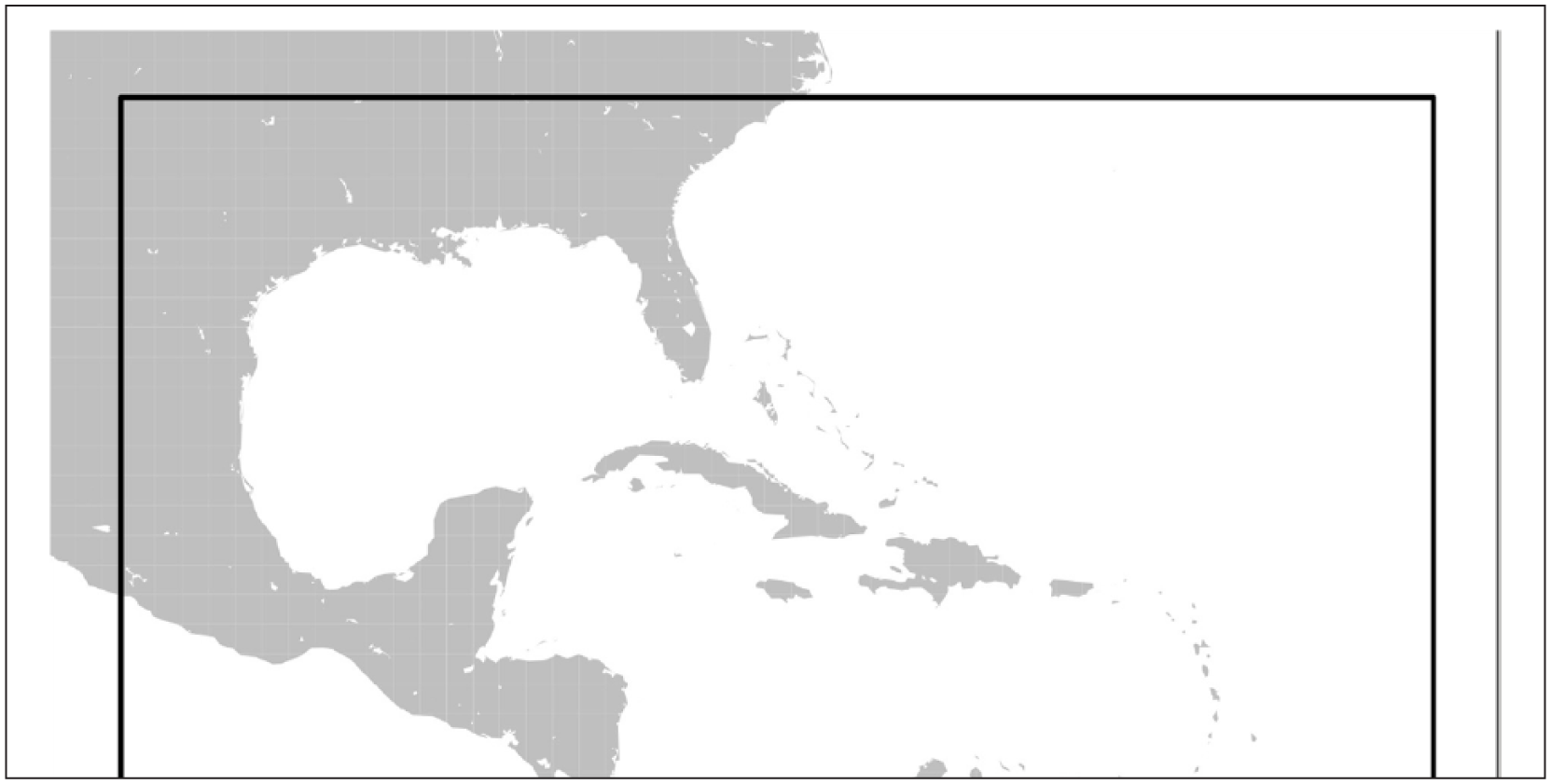
Domain used to run the RCM PRECIS.

The boundary conditions used were those from the GCM ECHAM5 and also from 6 of the 16 members of the set of perturbed physics HadCM3 CGM. In all cases, the emission scenario was SRES A1B, which may be considered as a moderate profile within the SRES (Nakicenovic and Swarts, 2000).

There are two kinds of methods to develop sets of models (model ensemble). The first is the multi-model method, which refers to collecting the outputs of models from different modeling centers and placing them within a repository to ensure access. In essence, this is an ad hoc method, in the sense that it is not completely designed to encompass the full range of uncertainty of models, but has the advantage of being a great “gene bank” of possible components of models (Collins et al., 2006). The other class has been called “Physically Disturbed” (PD), in which the structure of a single model is used and disturbances are introduced to model parameterization schemes (Murphy et al., 2004). Disturbances are introduced either on parameter or parameterization schemes themselves. The advantage of PD is that changes in the model formulations can be performed in a systematic way with great control over the design of the ensemble (Bezanilla et al., 2016).

Currently, the MetOffice at Hadley Centre is in a position to provide the boundary conditions for 17 members of a set of physically perturbed runs for use with the PRECIS RCM in order to allow users to generate a set of high-resolution regional simulations. However, in order to reduce the computational cost, only 6 of the 17 members are used in this work.

For the selection of the six members, the results presented by Sanderson (2011) were used to develop an expert judgment exercise (discussions and interactions between authors) within the Climate Modeling Group in the Caribbean.

The six members were selected carefully as those describing the widest possible range of future uncertainty as given by the values of climate sensitivity of each member. The sixth members of the subset was represented by the standard version of the model HadCM3, which is an unperturbed member. All experiments were performed at 10 m above sea level (ASL) to establish a comparison of the results with surface meteorological stations.

Dataset

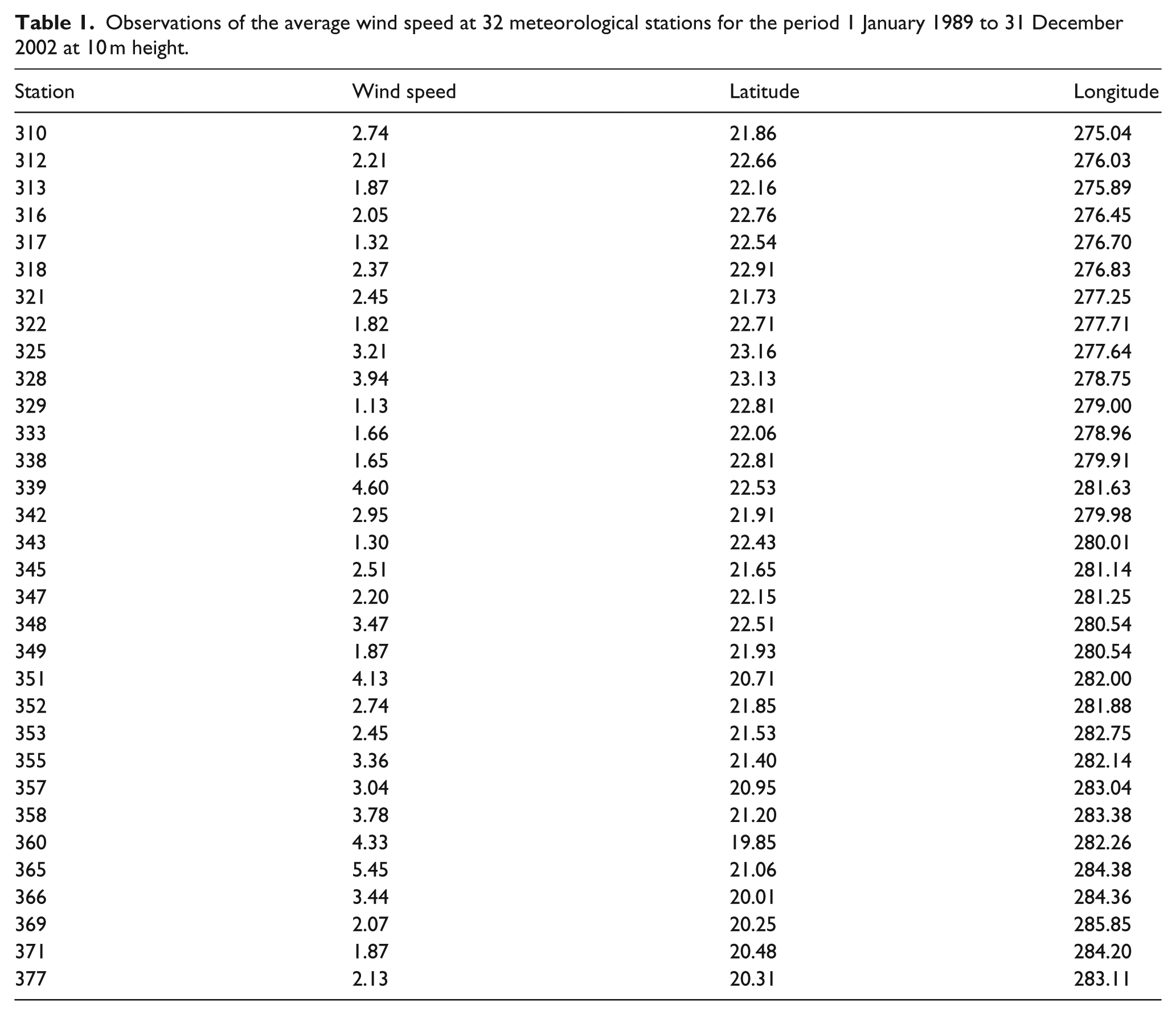
The dataset used for validation consists of 3-hourly observations of wind speed at 32 meteorological stations during the period 1 January 1961 to 31 December 2011 at 10 m height above ground level (AGL) (Table 1). The location of these meteorological stations is shown in Figure 2 where the dots refer to the meteorological stations used for validation. These data, including daily wind speed, estimated from the 3-hourly observations for the period 1 January 1989 to 31 December 2002, were compared with estimated wind from the PRECIS model fed by reanalysis data provided in section “Comparison between PRECIS model output and meteorological stations observation.” The wind power value is calculated using the expression

E_{1} = 0.5 ρ V^{3}

(1)

where the air density $ρ$ is assumed to be approximately 1.19 kg m⁻³ (Roque et al., 2018).

Table 1.

Observations of the average wind speed at 32 meteorological stations for the period 1 January 1989 to 31 December 2002 at 10 m height.

Station	Wind speed	Latitude	Longitude
310	2.74	21.86	275.04
312	2.21	22.66	276.03
313	1.87	22.16	275.89
316	2.05	22.76	276.45
317	1.32	22.54	276.70
318	2.37	22.91	276.83
321	2.45	21.73	277.25
322	1.82	22.71	277.71
325	3.21	23.16	277.64
328	3.94	23.13	278.75
329	1.13	22.81	279.00
333	1.66	22.06	278.96
338	1.65	22.81	279.91
339	4.60	22.53	281.63
342	2.95	21.91	279.98
343	1.30	22.43	280.01
345	2.51	21.65	281.14
347	2.20	22.15	281.25
348	3.47	22.51	280.54
349	1.87	21.93	280.54
351	4.13	20.71	282.00
352	2.74	21.85	281.88
353	2.45	21.53	282.75
355	3.36	21.40	282.14
357	3.04	20.95	283.04
358	3.78	21.20	283.38
360	4.33	19.85	282.26
365	5.45	21.06	284.38
366	3.44	20.01	284.36
369	2.07	20.25	285.85
371	1.87	20.48	284.20
377	2.13	20.31	283.11

Figure 2.

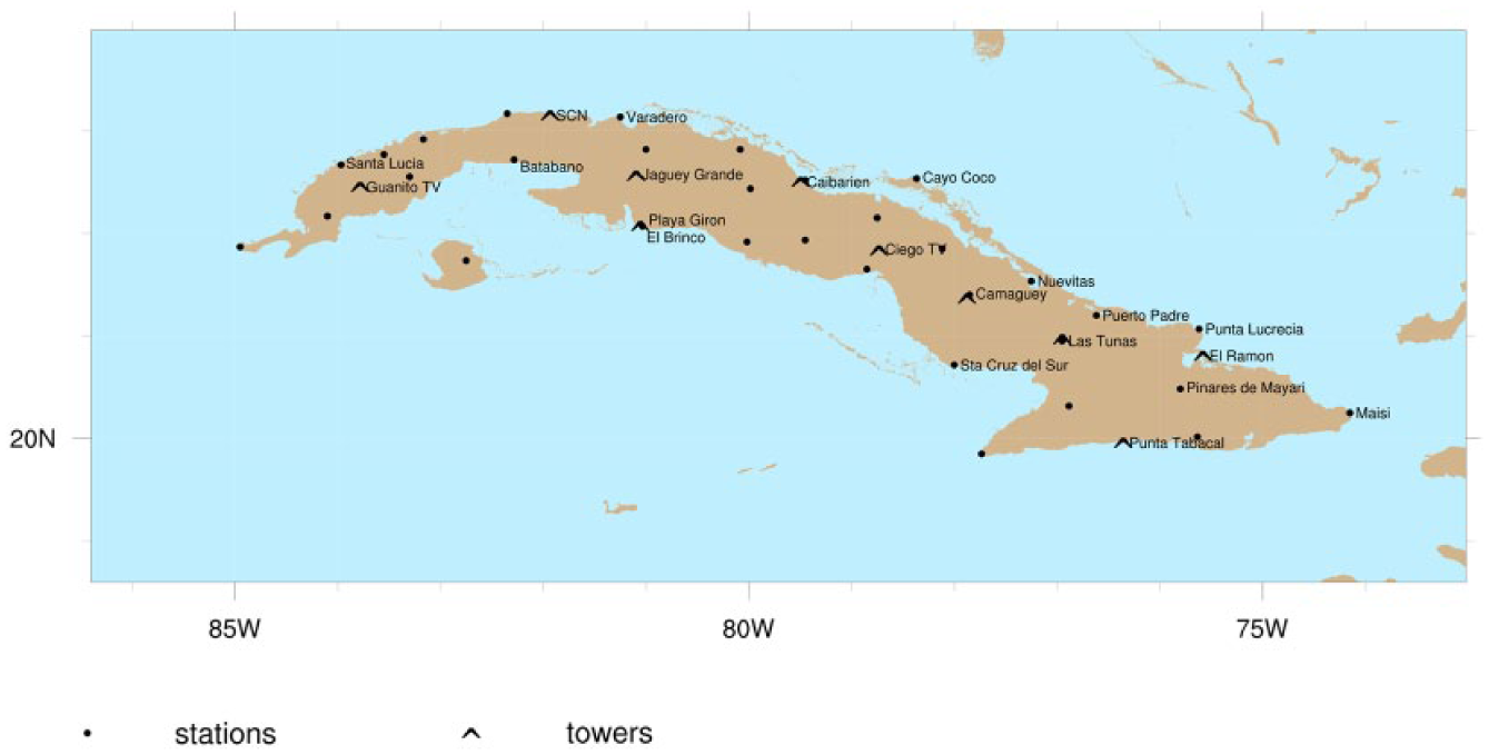
Position of meteorological stations used for model validation.

For this paper, the use of the PRECIS model followed the following procedure:

From the outputs of the model obtained with reanalysis data from the ERA-Interim, the daily averages of the values of the wind speed at 10 m AGL were taken for the period between 1 January 1989 and 31 December 2001.

In order to evaluate the model in the same period of time (1989–2001), we used the average daily values of the wind speed calculated from 3-hourly measurements at 32 of the 68 meteorological stations from INSMET surface network at 10 m height AGL (Table 1).

In order to estimate the temporal variation of the wind at regular intervals (30 years) for each grid point, the differences between the different future periods and the reference period (1961–1990) given by the seven different experiments (PRECIS driven by the six future climate scenarios plus ECHAM) were calculated, which eliminates the systematic error introduced by the model.

In order to verify whether the model simulated the wind magnitude correctly, the values obtained by the seven experiments were compared with the average real wind speed, obtained from the 3-hourly measurements for the 1961–2011 period. The comparison includes also the evaluation of the trend of the simulated versus observed wind speeds using the 10-year moving average.

Finally, in order to study the behavior of the wind resource in the future, the model daily values of the variation of the wind velocity for the surface level for the future periods F1 (2011–2040), F2 (2041–2070), and F3 (2071–2098) were compared with the outputs for the reference period.

Significance

The amount of variation, deviation from the average, or “spread” of the wind speed can be calculated using the standard deviation formula (2) (Schlotzhauer, 2007) for each grid point $i$ , where $V_{k i}$ is the value of the PRECIS wind speed for the ith grid point for day $k$ and ${\bar{V}}_{i}$ is the average speed for all days. $N$ is the total number of simulation days

σ_{i} = \sqrt{\frac{\sum_{k = 1}^{N} {(V_{k i} - {\bar{V}}_{i})}^{2}}{N}}

(2)

The significance level field in the ith grid point is calculated according to Bland and Altman (1996) using the following formula

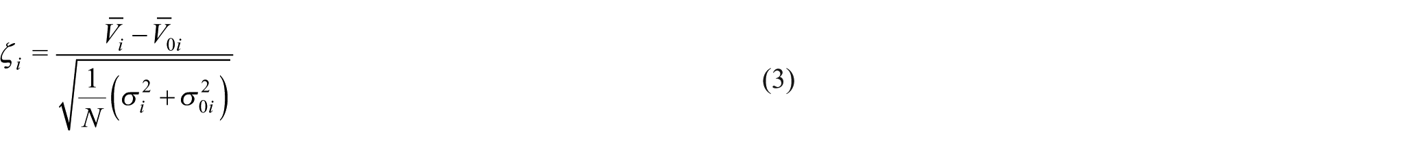
ζ_{i} = \frac{{\bar{V}}_{i} - {\bar{V}}_{0 i}}{\sqrt{\frac{1}{N} (σ_{i}^{2} + σ_{0 i}^{2})}}

(3)

where ${\bar{V}}_{0 i}$ is the average speed of the base period and $σ_{0 i}$ is the standard deviation of the base period.

After calculating the significance $ζ$ for each grid point, we keep only the values that are above the 95th percentile of the entire sample ( $ζ_{i} \geq 1.96$ ), and only those grid points are now taken into account to represent the wind speed bias.

Results

Comparison between PRECIS model output and meteorological station observation

In order to calculate the mean error of the estimated wind speed for the PRECIS RCM system (with respect to the actual measurements at the 32 meteorological stations) driven by reanalysis data (1989–2001), the estimated values at the grid point closest to the stations are used (Figure 3). The Cubic Spline method was used to interpolate the PRECIS model output in order to compare with the surface network station database. The mean absolute error (MAE) for all meteorological stations is 1.56 m s⁻¹. According to the findings in Figure 3, we can say that the PRECIS model tends to overestimate the wind speed, with some exceptions like Punta Lucrecia (365) and Gran Piedra (366). Bezanilla et al. (2016) argued that some of the main factors of the discrepancies in the calculations can be attributed to the size of the model horizontal grid.

Figure 3.

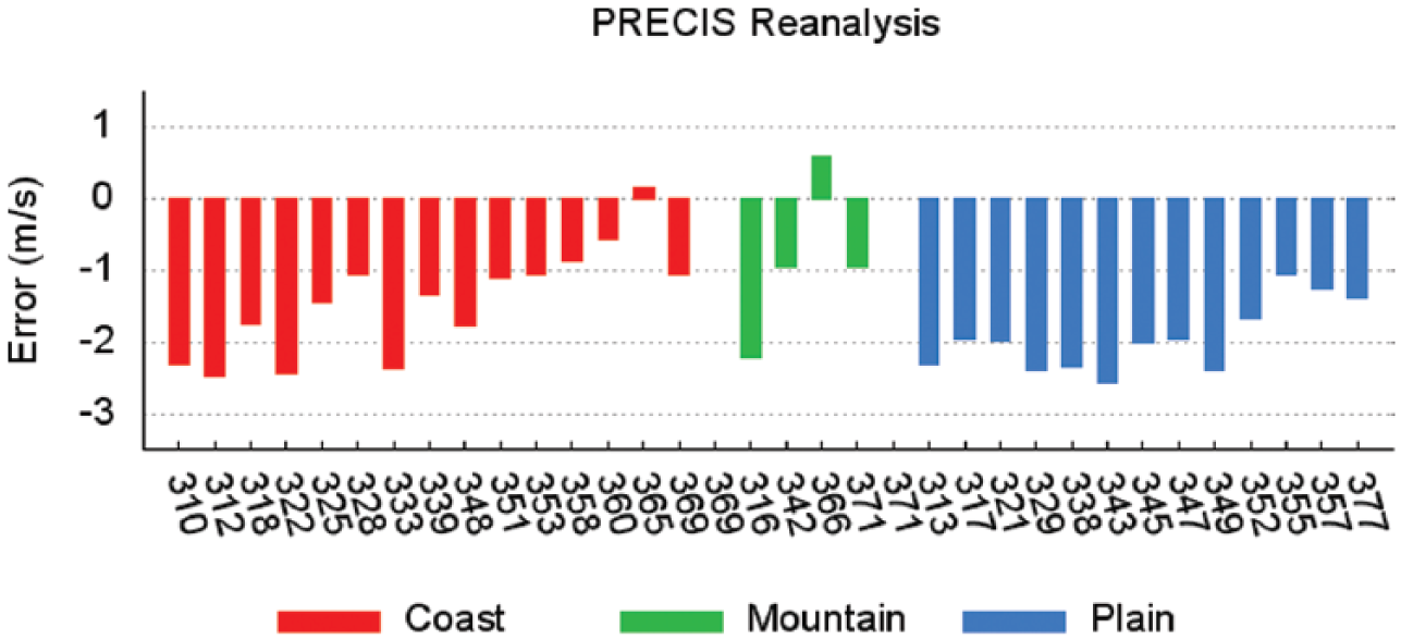
Mean error of the estimated wind speed for the PRECIS model driven by reanalysis data for the 32 meteorological stations selected. The results are shown depending on the type of land with bars red, green, and blue representing coastal, mountainous, and plain areas, respectively.

Figure 4 shows the comparison between the wind speed measured and that estimated by the PRECIS model. The scatter plot of this figure reveals that, in general, the model tends to overestimate the average wind speed near the surface.

Figure 4.

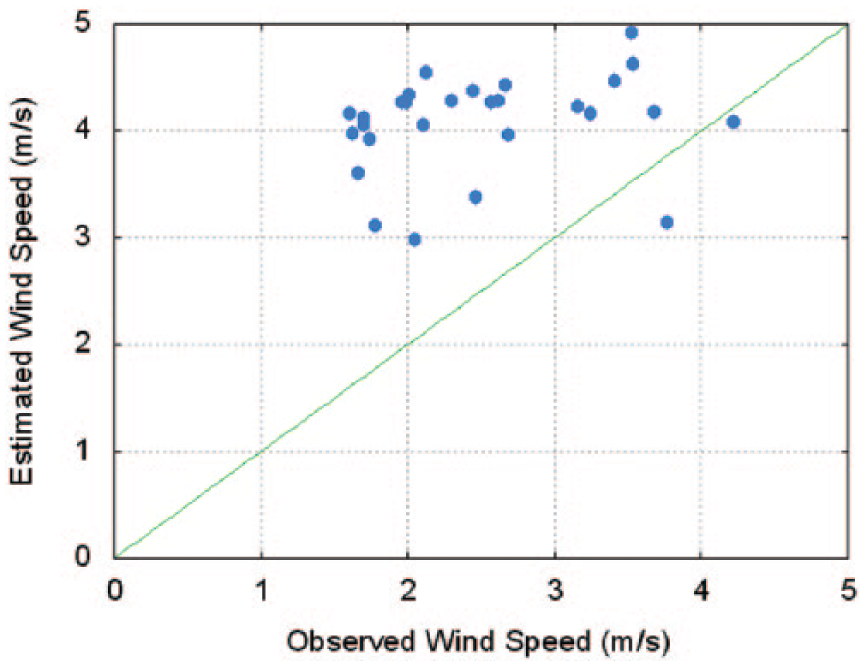
Scatter plots of observed versus estimated mean wind speed for the 32 meteorological stations.

Figure 5 shows the comparison between the MAE between the wind speed and the measured speed at 32 meteorological stations. Also in Figure 5, 10 meteorological stations exhibited absolute errors above 2.00 m s⁻¹, which were those located at Cabo San Antonio (310), Santa Lucía (312), Isabel Rubio (313), La Palma (316), Batabanó (322), Indio Hatuey (329), Playa Girón (333), Sagua La Grande (338), El Yabu (343), and Sancti Spíritus (349). The four stations with the fastest measured winds were those located at Punta de Maisí (4.26 m s⁻¹), Cayo Coco (4.23 m s⁻¹), Punta Lucrecia (4.22 m s⁻¹), and Varadero (4.08 m s⁻¹). For these stations in particular, the PRECIS model estimated the wind resource with reasonably accurate values of wind speed of 5.32, 5.55, 4.08, and 5.07 m s⁻¹, respectively. Of the remaining stations in which wind speed values were obtained below 2.50 m s⁻¹, six of them described MAE values below 1.00 m s⁻¹, and the rest (eight stations) showed MAE in the range of 1.01–1.94 m s⁻¹. The value of the average MAE was 1.56 m s⁻¹. In general, it can be concluded that the PRECIS model overestimated the wind resource, but reasonably estimated it in the coastal areas, with some exceptions such as Cabo San Antonio, Batabanó, and Playa Girón.

Figure 5.

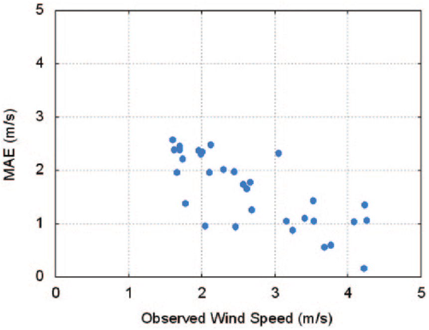
Scatter plots of the observed mean wind speed versus absolute error for the 32 meteorological stations.

To further facilitate the analysis of the results, the spatial distribution of the biases of the mean wind speed is shown in Figure 6.

Figure 6.

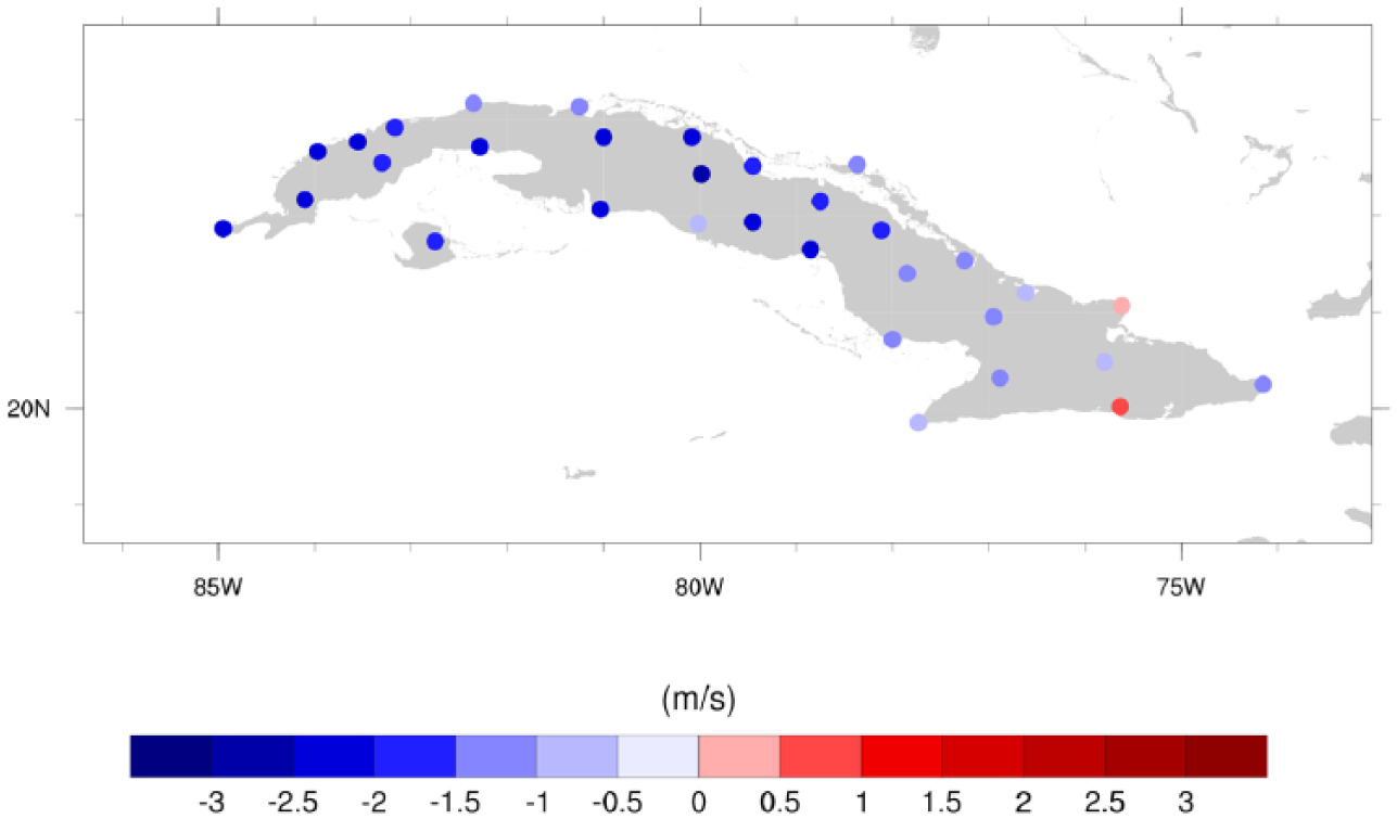
Map of Cuba showing the bias between the observed and estimated 10 m AGL mean wind speed.

To better understand the model performance, and its ability to represent the climatic variability of the wind, the stations in Casa Blanca (with the largest number of years of measurements) in Camagüey, Nuevitas, Puerto Padre, Punta Lucrecia, and Maisí were selected since they are related to the wind studies that are currently carried out in Cuba (Roque et al., 2018).

Time series were constructed using the PRECIS model for mean wind speed in different meteorological stations (black lines) and for wind speed (blue lines), in this case with the reanalysis data at 10 m height AGL for the period between 1 January 1989 and 31 December 2001 (Figure 7). The results indicate that despite the errors of the model, it is able to estimate reasonably well the trend in the wind time series for the selected meteorological stations.

Figure 7.

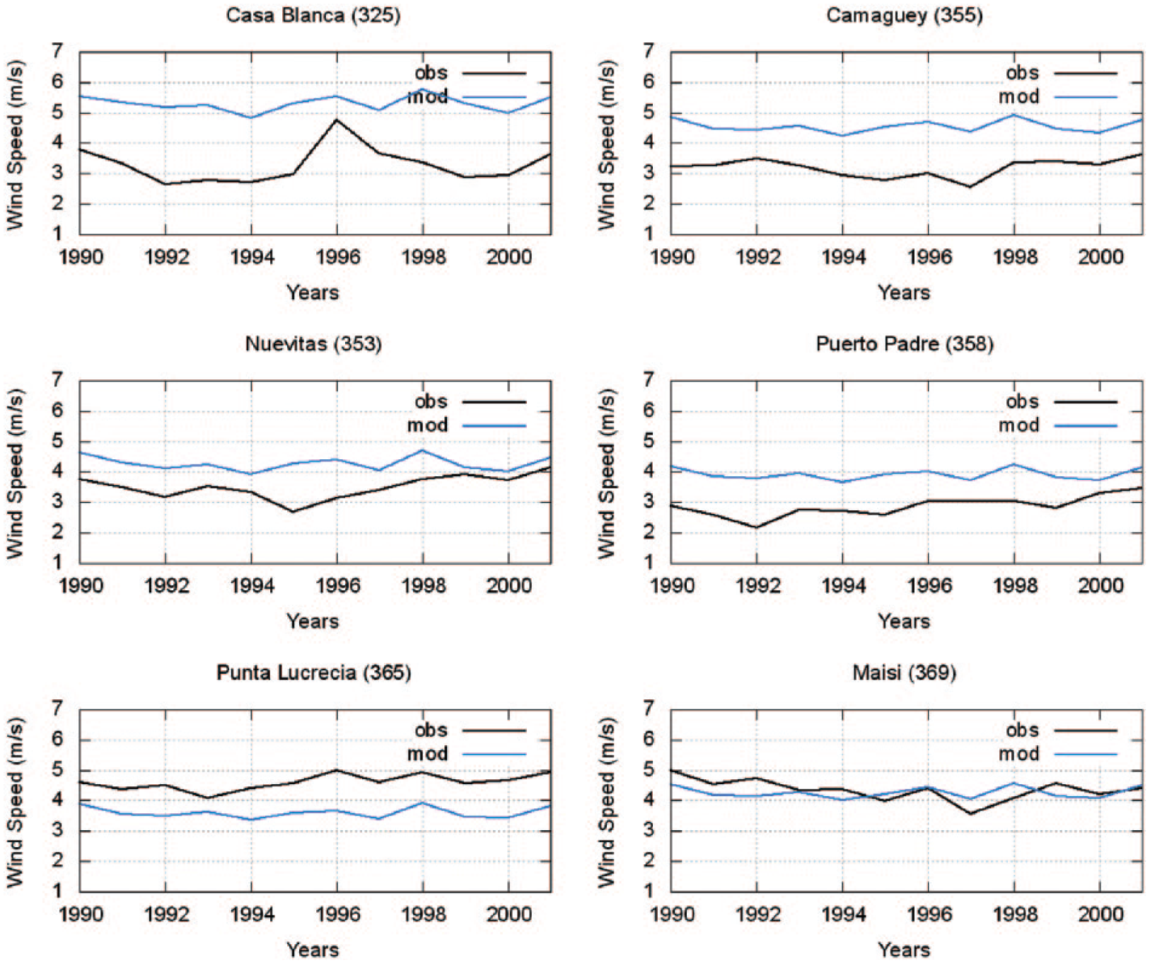
Time series constructed using the PRECIS model for wind speed (blue) and mean wind speed in different meteorological stations (black) at 10 m AGL.

Figure 8 shows the the mean wind speed for each of the periods selected with respect to the base period, taking into account the mean value of the ensemble, given the different scenarios. In this figure, a reinforcement of the magnitude of the wind can be seen, especially toward the second half of the century in regions where the largest wind resources in Cuba are currently located (Alonso et al., 2018; Roque et al., 2018). To assess the significance of this increase, the level of significance was calculated using the methodology described in section “Significance,” and the result is reflected in Figure 9. Setting an absolute threshold value of 1.96, corresponding to 95% of the interval of no significance, would help to identify regions where the increase obtained for the second half of the century is truly important. Filtering of these values is shown in Figure 10, with a significant increase for each of the periods with respect to the base period. It can be seen that for the periods 1991–2010 and F1, the average wind does not experience any change in its magnitude, and from the period F2, it begins to show a rising trend on the north coast from the central provinces to the east of the country, and this will further increase to the period F3. The expected increase in wind speed is between 0.1 and 0.4 m s⁻¹, and it may be higher for higher levels, if the vertical increase in wind speed in the atmospheric surface layer is taken into account (Emeis, 2013). The most relevant aspect of this result is that it can consolidate the current projection of the Cuban wind program until 2030, where the construction of 13 wind farms is proposed precisely in those regions where the increase in the wind speed is expected. Moreover, Cuba’s southern coast experienced a slight decrease in the values of wind speed that will be greater toward the Caribbean Sea.

Figure 8.

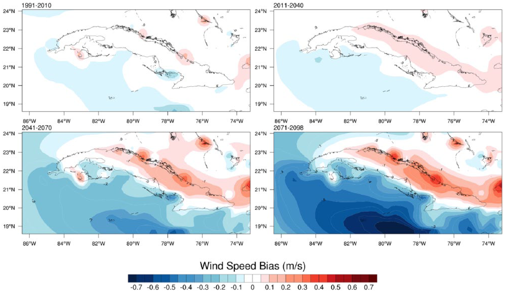
Wind speed bias for each of the periods selected, taking into account the average value of the ensemble, given the different scenarios.

Figure 9.

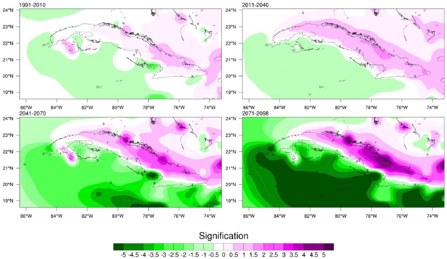
Level of significance between the base period and the various selected time periods.

Figure 10.

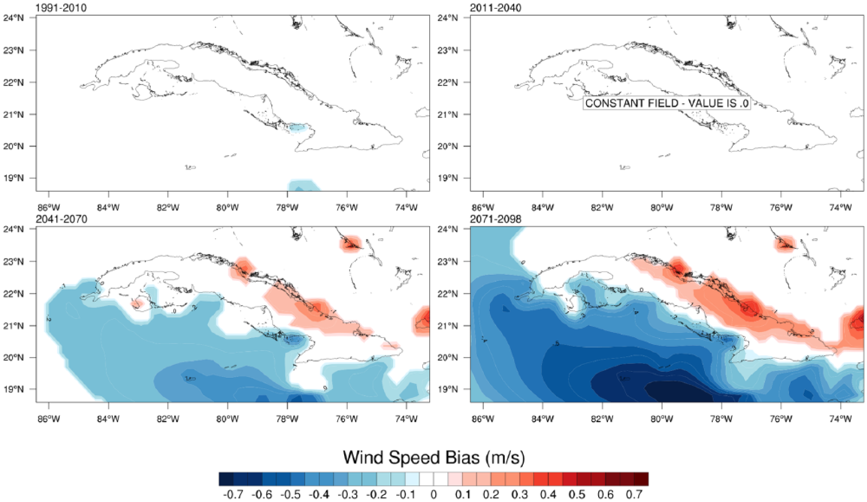
Wind speed bias between the base period and the various selected time periods.

In order to provide greater detail on the behavior found above, Figures 11 to 13 show the values of speed of average annual wind power density given by various experiments using the PRECIS model for Maisí stations, Punta Lucrecia, and Casa Blanca (three selected stations in Figure 7). In the case of the Maisí station, Figure 11 shows that the values of wind speed for all models are between 4.5 and 6.5 m s⁻¹ and power density values are between 150 and 450 W m⁻². The 10-year moving average shows a slight upward trend toward the end of the century. Moreover, in the Punta Lucrecia (Figure 12) station, it is seen that the values of wind speeds for all models are between 3.3 and 5 m s⁻¹ and the power density values are between 70 and 200 W m⁻². The 10-year moving average shows a slight upward trend toward the end of the century. This feature was also found for other stations in the eastern region. However, for the station Casa Blanca (Figure 13) located in the western region, no trend is displayed for wind speed or wind density power, corresponding this analysis with findings, in general, in Figure 10. Figures 14 to 16 show the distribution of the average annual wind frequency given by the ensemble of the PRECIS model (driven by the six future climate scenarios plus ECHAM) and the monthly distribution of the wind speed for Maisí stations, Punta Lucrecia, and Casa Blanca. The stations Maisí and Punta Lucrecia (Figures 14 and 15) show a slight upward trend in the distribution of the average annual wind frequency for values greater than 4 m s⁻¹ in the future periods (F2 and F3); this increase in the wind speed will be mainly reflected in the months of May to October. For the station Casa Blanca (Figure 16), there is no significant change in the distribution of the average annual wind frequency in the future.

Figure 11.

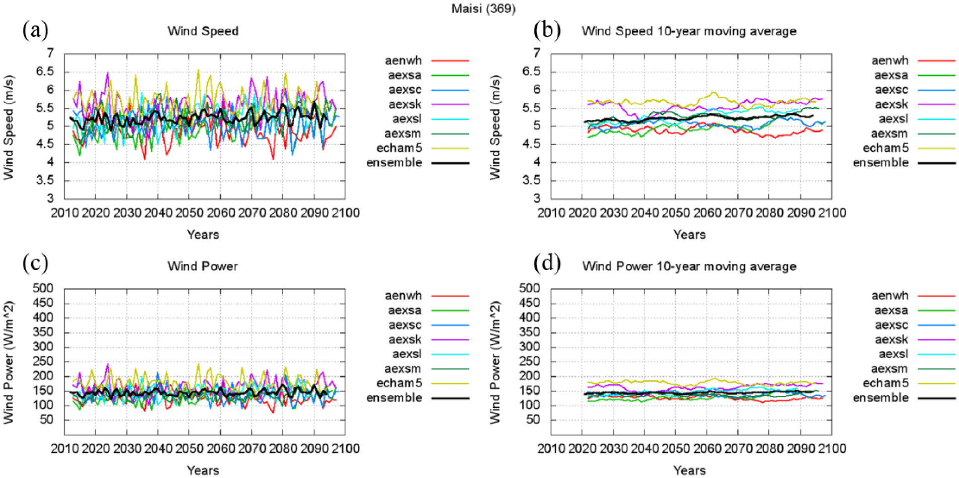
Maisí from 2011 to 2098: (a) speed of the average annual wind for each of the models (six scenarios PRECIS + ECHAM5), (b) 10-year moving average for the annual wind speed, (c) wind power, and (d) 10-year moving average for wind power.

Figure 12.

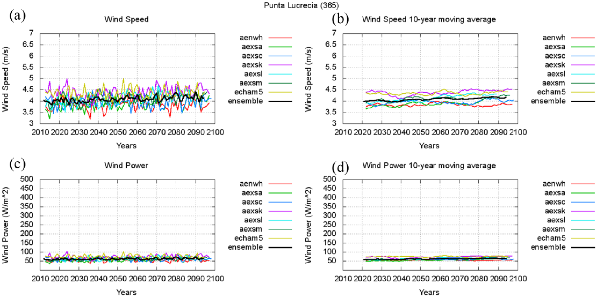
Punta Lucrecia form 2011 to 2098: (a) speed of the average annual wind for each of the models (six scenarios PRECIS + ECHAM5), (b) 10-year moving average for the annual wind speed, (c) wind power, and (d) 10-year moving average for wind power.

Figure 13.

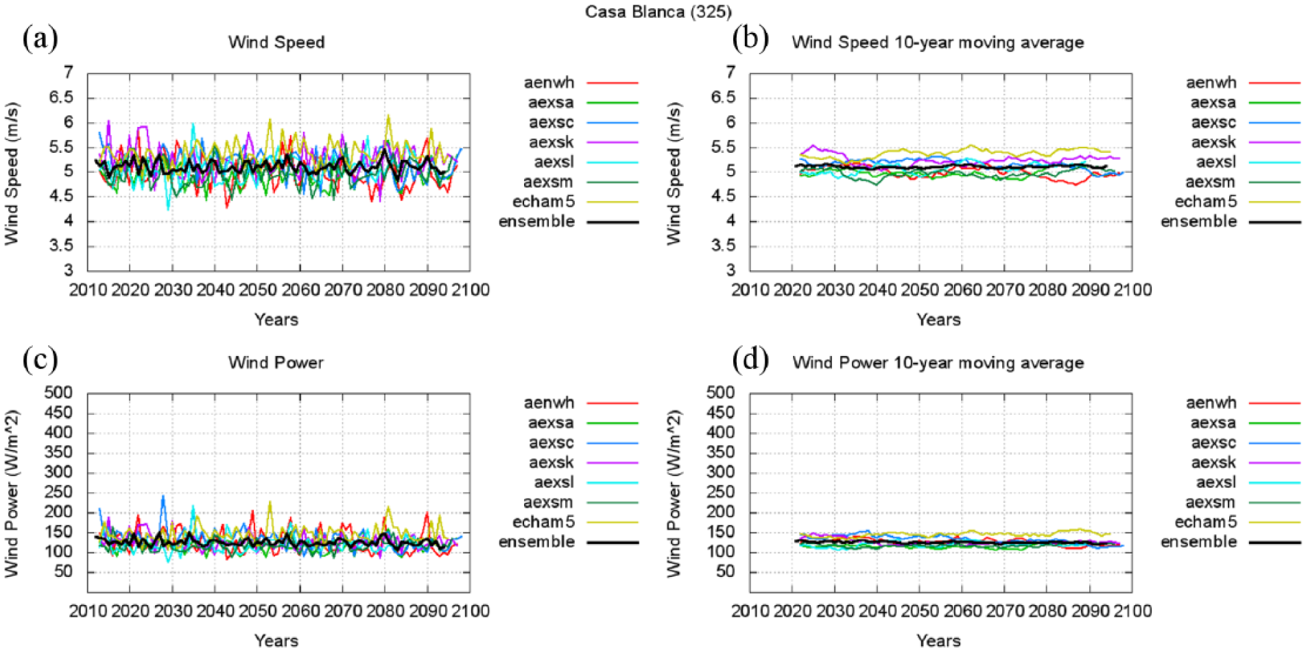
Casa Blanca from 2011 to 2098: (a) speed of the average annual wind for each of the models (six scenarios PRECIS + ECHAM5), (b) year moving average for the annual wind speed, (c) wind power, and (d) 10-year moving average for wind power.

Figure 14.

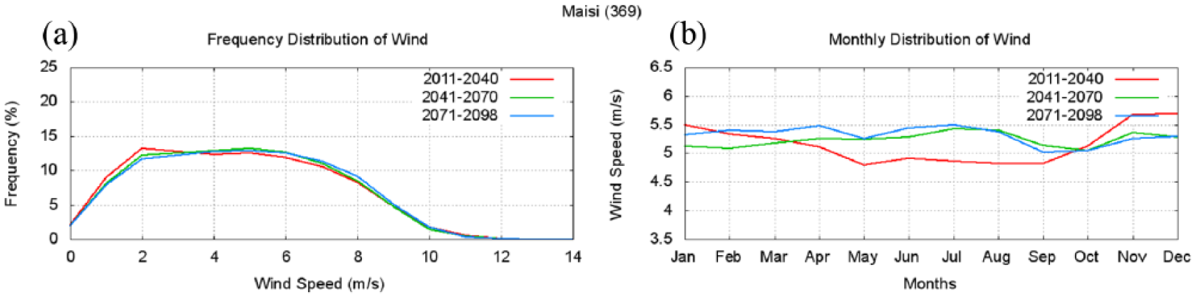
Maisí from 2011 to 2098: (a) distribution of average annual wind frequency for each of the models (six scenarios PRECIS + ECHAM5) and (b) monthly distribution of the wind speed.

Figure 15.

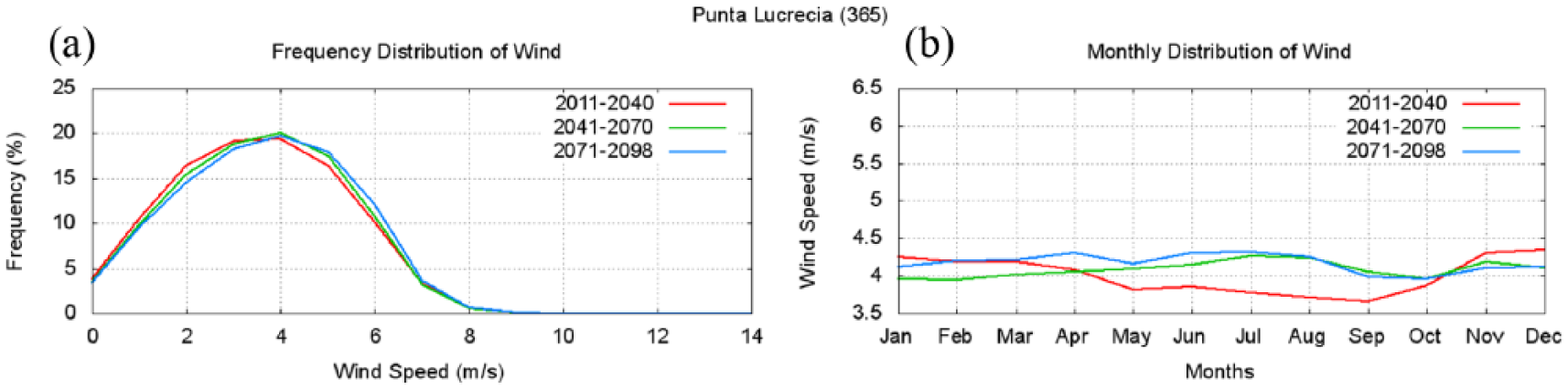
Punta Lucrecia from 2011 to 2098: (a) distribution of average annual wind frequency for each of the models (six scenarios PRECIS + ECHAM5) and (b) monthly distribution of the wind speed.

Figure 16.

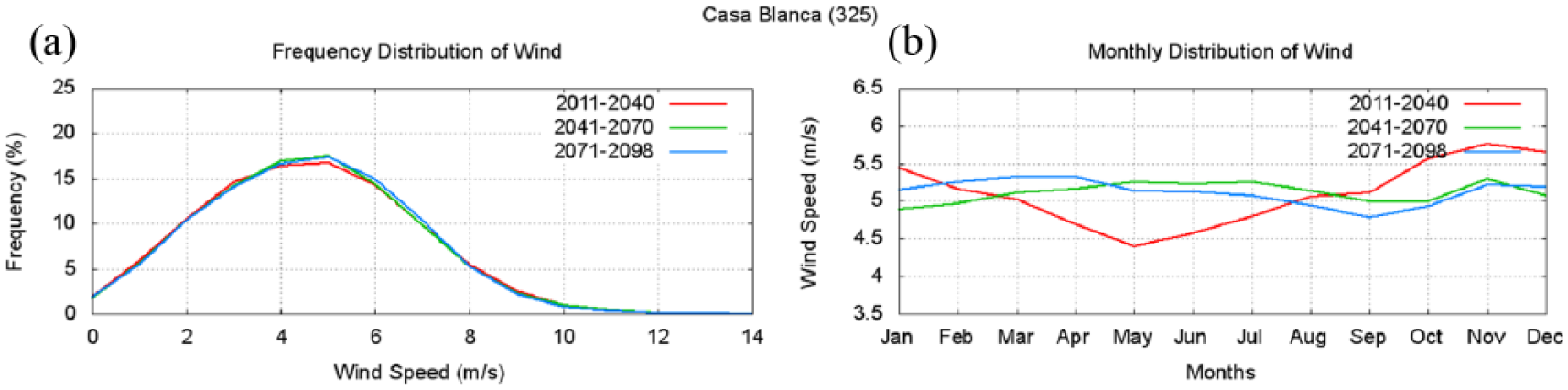
Casa Blanca from 2011 to 2098: (a) distribution of average annual wind frequency for each of the models (six scenarios PRECIS + ECHAM5) and (b) monthly distribution of the wind speed.

Future projection of the wind power of Cuba

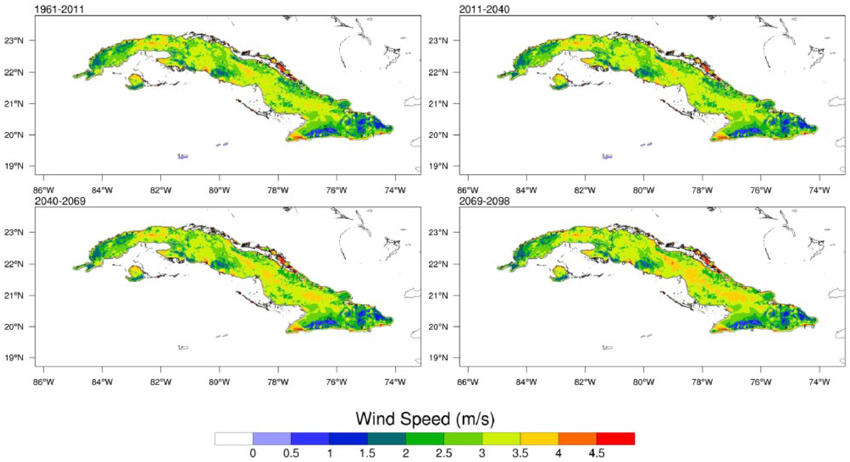
In this section, future projections are presented, which are based on estimates from the reference period (1961–1990) and changes in future periods (F1, F2, and F3), taking approximately intervals of 30 years as recommended by the World Meteorological Organization (WMO, 1989) for conducting the climatological studies. Figure 17 shows the average wind given by the ensemble using the PRECIS model for different periods selected. In this figure, it can be seen that on the north coast the highest values are obtained in correspondence with other works on the estimation of wind resources in Cuba (Alonso et al., 2018; Roque et al., 2018). Figure 18 is as Figure 17, but for the wind power given in W m⁻².

Figure 17.

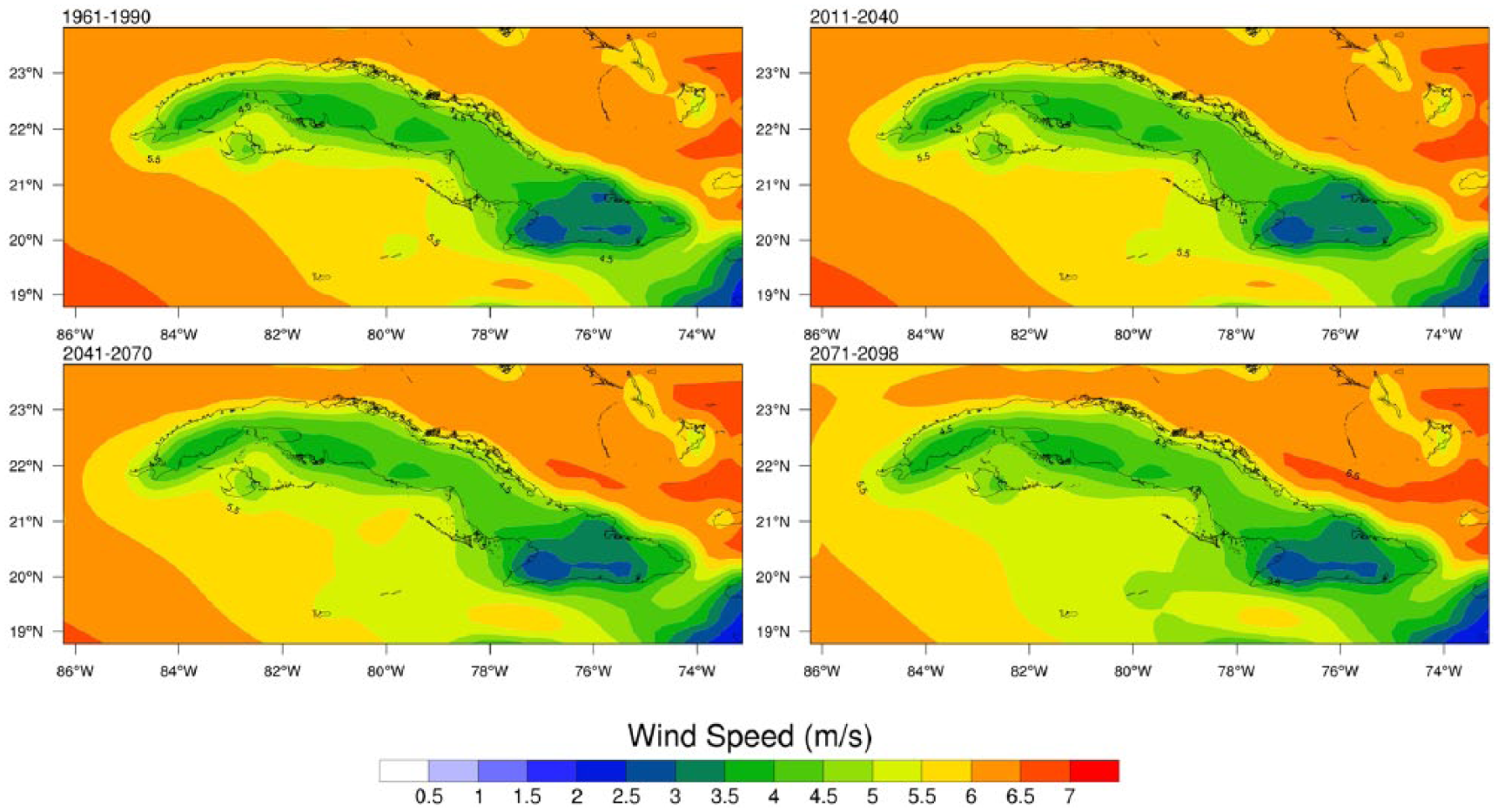
Average wind speed given by the ensemble using the PRECIS model for different selected periods. The values of the average wind speed are given in m⁻².

Figure 18.

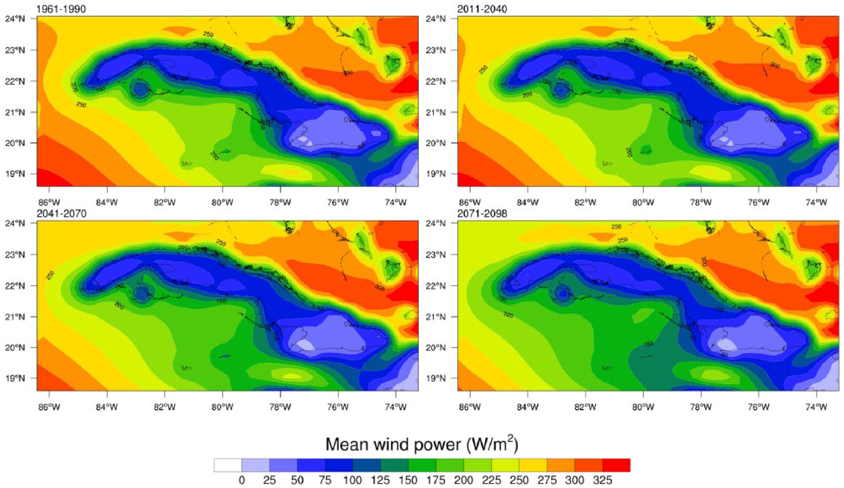
Average wind power given by the ensemble using the PRECIS model for different periods selected. The values of the average wind power are given in W m⁻².

In the previous section the regions where changes are significant from a statistical standpoint are identified. In regions where the changes are significant, this variation will be added to the wind speed outputs of the Numerical Wind Atlas of Cuba generated by Alonso et al. (2018) to estimate the values of wind speed in the three future periods. The values of wind speed in the mean wind speed map at 10 m ASL obtained by Alonso et al. (2018) (Figure 19) are enhanced by the increase in wind speed for each one of the periods already discussed previously in this paper (Figure 10). This increase in the wind speed obtained by PRECIS model is more accurate than the forecast of the model itself, so by subtracting the future outputs from the outputs of the base period the systematic error of the model is canceled (see Figure 3). Then by adding this increase to the current mean wind (here we assume as obtained by Alonso et al. (2018) in Figure 19), a better estimate of the values that wind speeds should reach in the next decades is obtained (Figure 20). Figure 20 shows the values of the wind speed in different future periods throughout the national territory (10 m height ASL), which has tremendous value for the wind energy industry in Cuba.

Figure 19.

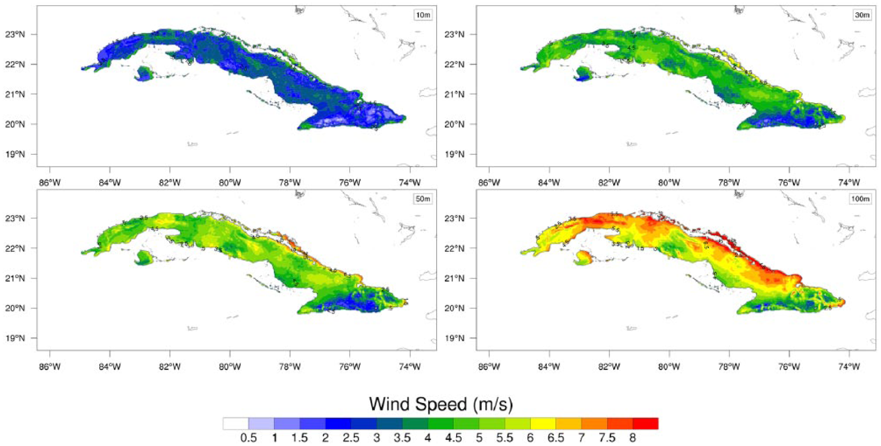
New Wind Atlas Cuba obtained by Alonso et al.’s (2018) at 10, 30, 50, and 100 m height AGL (2007–2009). The values of the average wind speed are given in m s⁻¹.

Figure 20.

Average wind generated by the model WEST-C (Figure 19) plus the increase in wind speed generated by PRECIS (Figure 10) at 10 m height AGL for the periods 1961–2011, 2011–2040, 2040–2069, and 2069–2098. The values of the average wind speed are given in m s⁻¹.

Conclusion and discussion

Wind energy resources assessment has always been a difficult challenge, even more when it comes to future predictions. Climate Change is a fundamental topic of the international scientific community due to the impacts that are expected, and it is necessary to anticipate in advance to act consequently. These impacts comprise all sectors of society, including the electricity sector, which is currently being introduced within the energy matrix of renewable energy resources in Cuba. For this reason, to have a tool capable of estimating the future behavior of the wind, with its uncertainties, is of great interest. In this work, all the verifications were carried out at 10 m height AGL where experimental and observational data were available. The absolute error of wind speed estimated by PRECIS model (Figure 3) is calculated using the Cubic Spline method to interpolate the model output in order to compare with the surface network station database. The results for this first experiment indicate that, overall, PRECIS overestimates the near-surface wind speed and the largest wind resources are obtained on coastal areas, at the top of the hills, and in plateaus. The largest discrepancies between observations and model are found at the stations with observed wind speed below 2.5 m s⁻¹ which are mainly located in coastal regions, areas of dense and high vegetation clusters, and narrow keys that were smoothed out by the model grid spacing. Future use of the coupled micro-mesoscale modeling component in PRECIS may be helpful to further improve the results. In the future, it is observed that the wind resource will be greater in the eastern and northern coast of the country, which is in agreement with other studies on estimation of the wind resource in Cuba. Compared with the baseline it is observed that the major changes will occur in the northeast coast of the country in the second half of this century, and these changes are statistically significant for an increase in the magnitude of the wind between 0.1 and 0.4 m s⁻¹ with a confidence level of 95% to 10 m height AGL, coinciding with the current projection of the Cuban wind program until 2030 where the construction of 13 new wind parks has been planned. The main recommendation that emerges from this work is to extend the spectrum of simulations, combining different GCMs and RCMs to have an adequate number of future simulations. This would allow us to reduce the uncertainty associated with the use of a single RCM combined with several global models. It would also allow us to create a probability distribution function and provide our results probabilistically rather than deterministically.

Footnotes

Declaration of conflicting interests

The author(s) declared no potential conflicts of interest with respect to the research, authorship, and/or publication of this article.

Funding

The author(s) received no financial support for the research, authorship, and/or publication of this article.

References

Alonso

Martinez

Roque

et al . (2018) A post-processing module based on Cressman’s Analysis to improve the Wind Energy Simulation Toolkit (WEST) mapping system. Wind Engineering. Available at: http://www.latestjournalarticles.com/default.asp?tab=3&camefrom=ENERGY&issn=0309-524X&eissn=blank

Angeles

Gonzalez

Erickson

et al . (2007) Predictions of change in the Caribbean region using global general circulation models. International Journal of Climatology 27: 555–569.

Balog

Ruti

Tobin

et al . (2016) A numerical approach for planning offshore wind farms from regional to local scales over the Mediterranean. Renewable Energy 85: 395–405.

Barstad

Sorteberg

Mesquita

(2012) Present and future offshore wind power potential in northern Europe based on downscaled global climate runs with adjusted SST and sea ice cover. Renewable Energy 44: 398–405.

Bezanilla

Centella

Roque

et al . (2016) Escenarios climáticos de alta resolucion sobre el Caribe usando el modelo PRECIS: Análisis preliminar sobre el comportamiento de dos fuentes renovables de energía en Cuba. Informe científico técnico, INSMET. Available at: http://scielo.sld.cu/scielo.php?script=sci_arttext&pid=S1815-59012018000200007

Bland

Altman

(1996) Statistics notes: Measurement error. British Medical Journal 313(7059): 744.

Campbell

Taylor

Stephenson

et al . (2010) Future climate of the Caribbean from a regional climate model. International Journal of Climatology 31: 1866–1878.

Centella

Bezanilla

Borrajero

et al . (2009) Escenarios Climáticos de Alta Resolución para la región de los Mares Interamericanos utilizando el Modelo PRECIS. Informe de Resultado Científico Instituto de Meteorología, p. 53.

Centella

Taylor

Bezanilla

et al . (2015) Assessing the effect of domain size over the Caribbean region using the PRECIS regional climate model. Climate Dynamics 44: 1901–1918.

10.

Collins

Booth

Harris

et al . (2006) Towards quantifying uncertainty in transient climate change. Climate Dynamics 27: 127–147.

11.

Da Silva

Banga

Alves

JMB

(2017) Modeling of wind resources on Mozambique considering a climate change scenario. Revista Brasileira de Meteorologia 32: 157–170.

12.

Diro

Rausher

Giorgi

et al . (2012) Sensitivity of seasonal climate and diurnal precipitation over Central America to land and sea surface schemes in RegCM4. Climate Research 52: 31–48.

13.

Emeis

(2013) Wind Energy Meteorology: Atmospheric Physics for Wind Power Generation. Berlin; Heidelberg: Springer-Verlag, p. 198 (Series: Green Energy and Technology).

14.

Fuentes-Franco

Coppola

Giorgi

et al . (2015) Inter-annual variability of precipitation over Southern Mexico and Central America and its relationship to sea surface temperature from a set of future projections from CMIP5 GCMs and RegCM4 CORDEX simulations. Climate Dynamics 45: 425–440.

15.

Hueging

Haas

Born

(2013) Regional changes in wind energy potential over Europe using regional climate model ensemble projections. Journal of Applied Meteorology and Climatology 52: 903–917.

16.

Jones

Noger

Hassell

et al . (2004) Generating High Resolution Climate Change Scenarios Using PRECIS. Exeter: Met Office Hadley Centre, p. 40.

17.

Karmalkar

Taylor

Campbell

et al . (2012) A review of observed and projected changes in climate for the Islands in the Caribbean. Atmósfera 26: 283–309.

18.

Martínez

Vichot

Bezanilla

et al . (2016) Performance of RegCM-4.3 over the Caribbean region using different configurations of the Tiedtke convective parameterization scheme. Revista de Climatología 16: 77–98.

19.

Matthew

Ohunakin

(2017) Simulating the effects of climate change and afforestation on wind power potential in Nigeria. Sustainable Energy Technologies and Assessments 22: 41–54.

20.

Murphy

Sexton

Barnett

et al . (2004) Quantification of modelling uncertainties in a large ensemble of climate change simulations. Nature 430: 768–772.

21.

Nakicenovic

Swarts

(2000) Special Report on Emissions Scenarios. A Special Report of Working Group III of the Intergovernmental Panel on Climate Change. Cambridge; New York: Cambridge University Press, p. 599.

22.

Pryor

Barthelmie

Clausen

et al . (2012a) Analyses of possible changes in intense and extreme wind speeds over northern Europe under climate change scenarios. Climate Dynamics 38: 189–208.

23.

Pryor

Nikulin

Jones

(2012b) Influence of spatial resolution on regional climate model derived wind climates. Journal of Geophysical Research 117: D03117.

24.

Romanic

Rasouli

Hangan

(2017) Urban wind resource assessment in changing climate: Case study. Wind Engineering 41: 3–12.

25.

Roque

Alonso

Martinez

et al . (2018) Application of the wind energy simulation toolkit in subtropical climates: Wind Atlas of Cuba. Wind Engineering (ISSN: 0309524X (Submitted)).

26.

Saarnak

Bergstrm

Sderberg

(2014) Uncertainties connected to long-term correction of wind observations. Wind Engineering 38(3): 233–248.

27.

Sanderson

(2011) A multimodel study of parametric uncertainty in predictions of climate response to rising greenhouse gas concentrations. Journal of Climate 24: 1362–1377.

28.

Schlotzhauer

(2007) Elementary Statistics Using JMP (ed. PAP/CDR). Cary, NC: SAS Institute (SAS Press), pp. 166–169.

29.

Simmons

Burridge

(1981) An energy and angular-momentum conserving vertical finite difference scheme and hybrid vertical coordinates. Monthly Weather Review 109: 758–766.

30.

Soldatenko

Karlin

(2014) The climate change impact on Russia wind energy resource: Current areas of research. Energy and Power Engineering 6: 371–385.

31.

Taylor

Meehl

RSG

(2012) An overview of CMIP5 and the experiment design. Bulletin of the American Meteorological Society 93(4): 485–498.

32.

Vautard

Thais

Tobin

et al . (2014) Regional climate model simulations indicate limited climatic impacts by operational and planned European wind farms. Nature Communications 5: 3196.

33.

Vichot

Martínez

Centella

et al . (2014) Sensibilidad al cambio de dominio y resolución de tres configuraciones del modelo climático regional RegCM 4.3 para la región de América Central y el Caribe. Revista de Climatología 14: 45–62.

34.

World Meteorological Organization (WMO) (1989) Calculation of monthly and annual 30-year standard normals (WCDP Series). World Meteorological Organization. Available at: https://books.google.com.cu/books?id=z9FonAEACAAJ

35.

Yao

Huang

Lin

(2012) Climate change impacts on Ontario wind power resource. Environmental Systems Research 1: 2.

36.

Benoit

Girard

et al . (2006) Wind Energy Simulation Toolkit (WEST): A wind mapping system for use by the wind-energy industry. Wind Engineering 30: 15–33.