Weather research & forecasting model and MERRA-2 data for wind energy evaluation at different altitudes in Bolivia

Abstract

Wind energy is one of the most promising alternatives for a clean and ecological electricity generation. However, the implementation of efficient wind farms requires accurate data and measurements. This work analyses the MERRA-2 satellite datasets to compare and complement it with WRF simulations in different regions and altitudes in Bolivia, such as the Altiplano, Amazon and Chaco. A 41 years of hourly wind speed from MERRA-2 was used to analyze wind averages and characteristics over the year. WRF simulations for representative months were used to analyze wind shear and wind flows along Bolivia. The main results are related to wind speed index in different sites which varied between 0.90 and 1.09 and the periods of high wind speeds that is May—October in the Altiplano, and June—December in the Amazon and Chaco. However, the main findings are the differences between MERRA-2 data and WRF simulations that is linked to the topography of the sites in study.

Keywords

Wind energy numerical weather prediction WRF MERRA-2 Bolivia

Introduction

Wind speed assessment (WSA) is a key factor for wind energy prospection, feasibility analysis, and implementation (Aldeman et al., 2019). WSA is the base of wind energy resource, wind power potential, wind farm projects, and also for understanding of the meteorology on-site. Commonly, the WSA is obtained by measuring wind speed with meteorological towers and performing different equations, these could be obtained from private companies or national weather services. However, many countries have limitations for accurate measurements of wind speed for wind energy purposes, due to the wind power is a function of the cube of wind speed and it depends of the altitude from the ground. Additionally, meteorological towers are expensive and for an accurate WSA many towers would be required. For these reasons, limited measurements and expensive equipment, Numerical Weather Prediction (NWP) models and global re-analysis data are important alternatives (Al-Yahyai et al., 2010; Gruber et al., 2019).

NWP models consist on solving Navier-Stokes equations of the atmosphere interaction with land surface and, for this reason, there are several applications, such as forecast of weather, air-quality, and hydrological phenomena. However, NWP models need initial and boundary conditions to solve their equations, and global re-analysis data are used for this objective (Bauer et al., 2015; Olson et al., 2019). Furthermore, the Modern-Era Retrospective Analysis for Research and Applications, version 2 (MERRA-2) is one the most promising global re-analysis data, which contains meteorological data since 1980 (Gelaro et al., 2017). MERRA-2 have been used for wind energy analysis in Pakistan (Rabbani and Zeeshan, 2020), Mexico (Perea-Moreno et al., 2019), and Brazil (Olson et al., 2019). Although, MERRA-2 is very useful in climate analysis, the results should be taken cautiously, due to correlation coefficients (R) of MERRA-2 with measurements varied between 0.17 and 0.75 (Rabbani and Zeeshan, 2020). On the other hand, Weather Research and Forecasting (WRF) is one of the most important NWP models and it has been applied in atmospheric research and operational forecasting (Skamarock et al., 2008). WRF has been used for wind speed analysis (Franco et al., 2020), wind resource assessment (Penchah and Malakooti, 2020), wind power forecasting (Hodge et al., 2012; Mamani and Hendrick (2019). Additionally, WRF is effective for improving the spatio-temporal resolution of data, and this aspect is relevant for countries as Bolivia, considering the limited meteorological towers and the large territory of the country.

Although, NWP models and global re-analysis data can be used for WSA the accuracy and limitations should be evaluated. WRF model has been evaluated in different regions of the world and under different meteorological conditions, the main limitations are related to the sensitivity of the physics schemes in relation to the variable to predict and the site (García-Díez et al., 2013). On the other hand, MERRA-2 registers the data each 0.5° × 0.5° grids and in the wind speed is estimated indirectly by tracking features (clouds and water vapor) (McCarty et al., 2016). Already, 3TIER (2009) produced a Wind Atlas of Bolivia using WRF v3.0 simulating a complete year selected randomly between 1998 and 2007. However, the validation was a problem due to scarcity of measurements in the period of the simulations; and data from meteorological towers from northern Chile were considered for that purpose.

Bolivia is located in the center of South America surrounded by Argentina, Brazil, Chile, Paraguay, and Peru. According its position, the country has different meteorological and topographic conditions and for the purpose of this work, it could be divided in three regions: Amazon at the East, Andes at the West, and Chaco at the South (See Figure 1).The Amazon is characterized by large forests, high humidity and 300 m above sea level (masl) of altitude; the Andes could be divided in two sub-regions: Altiplano (Western) and Eastern Bolivian High, the mean altitude is 3900 and 2500 masl, respectively (Garreaud et al., 2009). Finally, the Chaco is characterized by high temperature, low precipitation and mean altitude of 400 masl (Aparicio-Effen et al., 2016).

Figure 1.

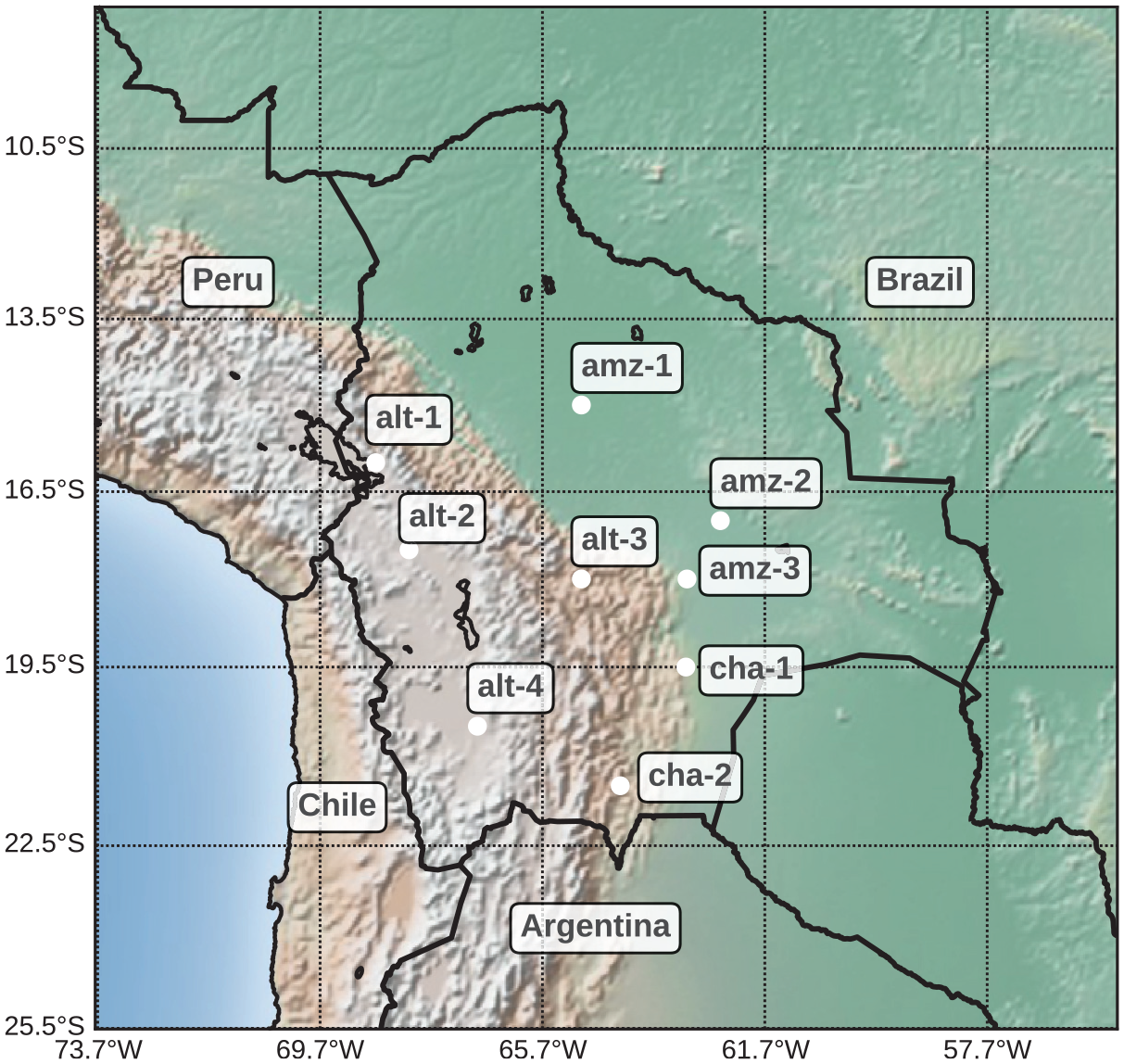
Sites of study in Bolivia.

For the sustainable energetic development of Bolivia a wind farm has been installed in the Eastern Bolivian High (Mamani et al., 2018), and others are under construction in the Amazon and the Chaco (Rojas Candia et al., 2019). However, additional knowledge related to wind speed assessment, wind speed index, wind speed variability, wind climatology, wind characteristics and wind data are required for wind energy operation, projection, integration to the Bolivian interconnected system and implementation of wind energy systems in microgrids (Balderrama et al., 2019).

This work evaluates MERRA-2 wind speed dataset to generate wind speed index, wind variability, wind characteristics for different altitudes and regions of Bolivia, the analysis covers the period 1980-2020. Then, WRF simulations of representative months are compared with MERRA-2 wind speed, and from WRF simulations wind shear is evaluated.

Methodology

Wind speed index and power spectrum density using MERRA-2 data

The wind speed index along Bolivia was evaluated using MERRA-2 data corresponding to 41 years of hourly wind speed. The yearly wind speed index was computed as the yearly mean wind speed divided by the mean wind speed of the 41 years between 1980 and 2020, as is shown in equation (1). The sites of analysis were selected in function of the topographic and meteorological conditions of Bolivia. These topographic conditions could be divided in the Andes, Amazon, and Chaco. The sites selected were four in the Andes, three in the Amazon, and two in the Chaco. The sites names, coordinates and site codes are in Table 1 and their positions in Figure 1. The reanalysis data MERRA-2 (Gelaro et al., 2017) was used for the different sites summarized in the Table 1. Additional techniques were used to evaluate the different wind characteristics along the country, such as the power spectrum density (PSD), long-term analysis of temperature and wind speed; and wind speed by month. However, this analysis was developed selecting at least one site per region as representatives. In the Altiplano, Amazon and Chaco were selected alt-2, amz-3, and cha-2, respectively. These sites were selected due to geographically are closer to the center of each region, also because these have been considered for future wind energy projects. The PSD was computed with the whole MERRA-2 dataset and using Welch’s method. For the long-term analysis, annual averages were used for a linear regression in the period 1980–2020 for temperature and wind speed. Finally, the monthly mean wind speed are plotted and analyzed with electricity demand in Bolivia, data extracted from CNDC (2010) web page. The purpose is to compare the monthly wind speed index with the electricity demand in Bolivia.

WS I_{year} = \frac{\frac{1}{m} \sum_{i = year}^{year + 1} Wind spee d_{i}}{\frac{1}{n} \sum_{j = 1}^{n} Wind spee d_{j}}

(1)

Where:

m = 8760 or 8784 (Leap years)

n = 359424

Table 1.

Sites for study.

Site code	Name	Latitude	Longitude	Altitude*	Terrain
alt-1	Achacachi	S16.00	W68.75	3951	Complex
alt-2	Patacamaya	S17.50	W68.12	3932	Flat
alt-3	Qollpana	S18.00	W65.00	2830	Complex
alt-4	Uyuni	S20.50	W66.87	3690	Flat
amz-1	Trinidad	S15.00	W65.00	158	Flat
amz-2	San Julian	S17.00	W62.50	255	Flat
amz-3	Santa Cruz	S18.00	W63.12	463	Flat
cha-1	El Espino	S19.50	W63.12	770	Flat
cha-2	La Ventolera	S21.50	W64.37	2311	Complex

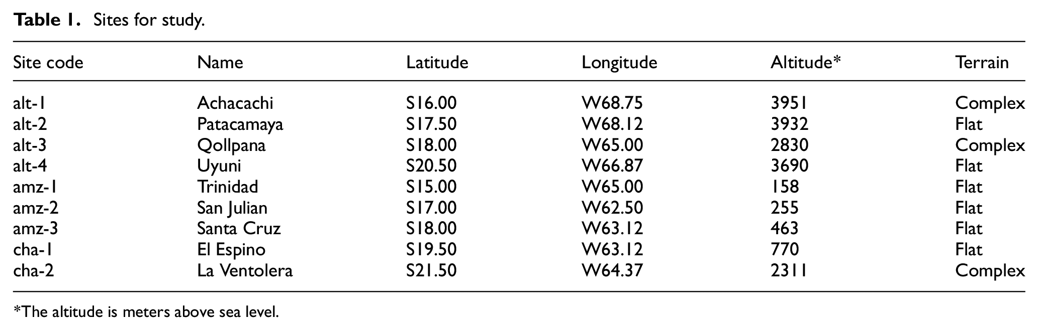
The altitude is meters above sea level.

WRF simulations and post-processing

WRF simulations were used for wind shear estimation, and to construct a wind map with wind vectors in Bolivia. The simulations were executed using WRF-ARW v3.5.1 with a domain size of 100 grids × 100 grids (17.631 S, 65.279 W as center of the domain), 30 km of grid spacing, and 53 vertical levels. The physics models were configured with Thompson scheme (Thompson et al., 2008) (microphysics), RRTMG schemes (Iacono et al., 2008) (shortwave and longwave radiation), and Yonsei University scheme (Hong et al., 2006) (PBL). The simulation consisted in 4 months of the different seasons of the year, March (2018), June (2018), September (2018), and December (2016), corresponding to the southern Autumn, Winter, Spring, and Summer, respectively; and the results of the simulations were saved every hour. The wind shear ( $γ$ ) represents the gradient of the wind speed in function of the altitude from ground; and depends on terrain conditions, sea breeze, and different weather conditions. The wind shear ( $γ$ ) was calculated every hour using linear regression from a linearized equation of the power law, shown in equation (2), then averaged by month. The regression was computed using 12 levels of wind speed at altitudes 4.4, 8.9, 13.3, 19.6, 26.8, 33.9, 44.7, 56.4, 67.1, 85.1, 98.7, 112.2 m above the ground. The wind vectors were build using the vectors spaced every 60 km at 85 m above the ground and for every season of the year.

u = u_{ref} (\frac{z}{z_{ref}})^{γ}

(2)

Results and discussion

Wind variability and wind speed index in Bolivia

The wind speed indexes are shown in two formats: figure and table. Figure 2 shows 41 years of the three regions, such as Altiplano, Amazon, and Chaco. Table 2 shows the wind speed index of all sites of study during the last 11 years.

Figure 2.

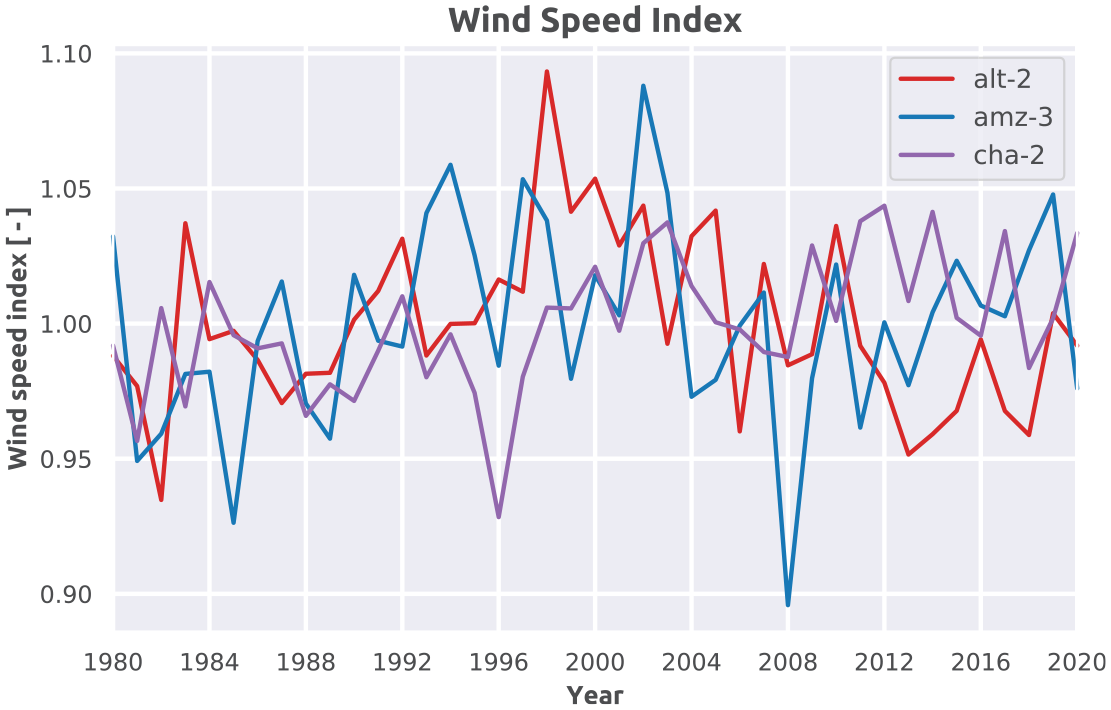
Wind speed index in three representatives sites. Altiplano (alt-2), Amazon (amz-3) and Chaco (cha-2).

Table 2.

Wind speed index of last 11 years.

Site	Mean*	2010	2011	2012	2013	2014	2015	2016	2017	2018	2019	2020
alt-1	4.24	0.989	1.011	0.997	0.966	0.983	0.989	0.955	1.010	0.976	1.043	1.024
alt-2	4.53	1.036	0.992	0.978	0.952	0.959	0.968	0.994	0.968	0.959	1.004	0.992
alt-3	4.71	1.007	0.945	1.002	0.945	0.975	1.036	0.997	0.995	0.981	1.045	0.968
alt-4	4.86	1.065	1.027	0.944	0.997	1.012	1.039	1.050	1.037	0.969	0.997	1.051
amz-1	3.67	1.081	0.967	0.963	0.933	0.998	0.928	0.997	0.960	0.960	0.990	0.943
amz-2	3.52	1.054	0.999	1.000	0.984	1.003	1.004	1.039	0.991	1.013	1.021	0.953
amz-3	6.62	1.022	0.962	1.000	0.977	1.004	1.023	1.007	1.003	1.027	1.048	0.976
cha-1	6.76	0.991	0.938	1.023	0.935	0.986	1.004	0.965	1.002	0.981	1.027	0.993
cha-2	3.95	1.001	1.038	1.044	1.008	1.041	1.002	0.996	1.034	0.984	1.002	1.034

Mean wind speed of the site in m/s.

Figure 2 displays the wind speed index on alt-2 (Patacamaya), amz-3 (Santa Cruz), and cha-1 (La Ventolera) as representatives of the different regions in Bolivia. The minimum wind speed index are on years 1986, 1996, and 2008; and the maximum are on years 1994, 1998, and 2002. Those years coincide with years of moderate ENSO phenomenon which are evaluated using the Oceanic Niño Index (ONI). The ONI index is a technique to identify the El Niño-Southern Oscilation (ENSO) years. The ENSO is defined as a periodical variation of the surface temperature over the tropical Pacific Ocean and this phenomenon affects the precipitation variability of the Bolivian Altipliano. El Niño (positive index) and La Niña (negative index), according their values those ENSO years could be considered weak (0.5 ≤ ONI ≤ 0.99), moderate (1 ≤ ONI ≤ 1.4) and strong (ONI ≥ 1.5) (Canedo-Rosso et al., 2019). The years of minimum wind speed index 1986, 1996 and 2008 have ONI of 1.3, −1.0, and −1.5, respectively; and the years of maximum wind speed index 1994, 1998, and 2002 have ONI of 1.1, −1.5, and 1.3, respectively (Null, 2000). Although, the minimum and maximum wind speed indexes coincide with ENSO years, these are not consistent with El Niño or La Niña events because positive and negative ONI indexes are in both, minimum and maximum. However, these results are consistent with Garreaud and Aceituno (2001) that consider inter-annual variability has more influence in the climate over the Altiplano than ENSO by itself. For example, in the Altiplano wind speed index varies periodically every 3 and 10 years, in the Amazon regions every 2.5 and 4 years, and in the Chaco every 3 years (Figure 2). However, there is an increasing wind speed index since 1980 until the period 1998–2002, after that the wind speed index decreases until 2010. Finally, since 2002 the wind speed index in the Altiplano (alt-2) continues decreasing, in the Amazon (amz-3) slightly increases and in the Chaco (cha-2) keeps most of the years higher than 1.

Table 2 displays the wind speed index of all the sites analyzed in this work. As Figure 2 shows since 2010 the wind speed index varies between 0.95 and 1.05. However, the wind speed index in the Amazon and the Chaco is most of the years higher than 1 and in the Altiplano is below 1. Additionally, these wind speed indexes shows different variability among Altiplano, Amazon, and the Chaco; this characteristic represents an advantage under a high wind energy penetration in the Bolivian interconnected system because, if there is one year with low wind speed in the Altiplano, the high wind speed in the Amazon and the Chaco compensates that insufficiency. Also that hypotheses could be supported by Figure 3 due to in January the Amazon (amz-3) has a wind speed index of 1 and in the Altiplano and the Chaco those are 0.92 and 0.94, respectively. The site alt-3 corresponds to Qollpana wind farm (the unique working wind farm in Bolivia) (Mamani et al., 2018) and even this site is over a mountainous region and 2800 masl its wind characteristics are quite similar to the Amazon regions. This is due to Qollpana wind farm is close to Amazon region and the wind characteristics of the Amazon influences directly to the closest mountainous region of the Andes (Table 2).

Figure 3.

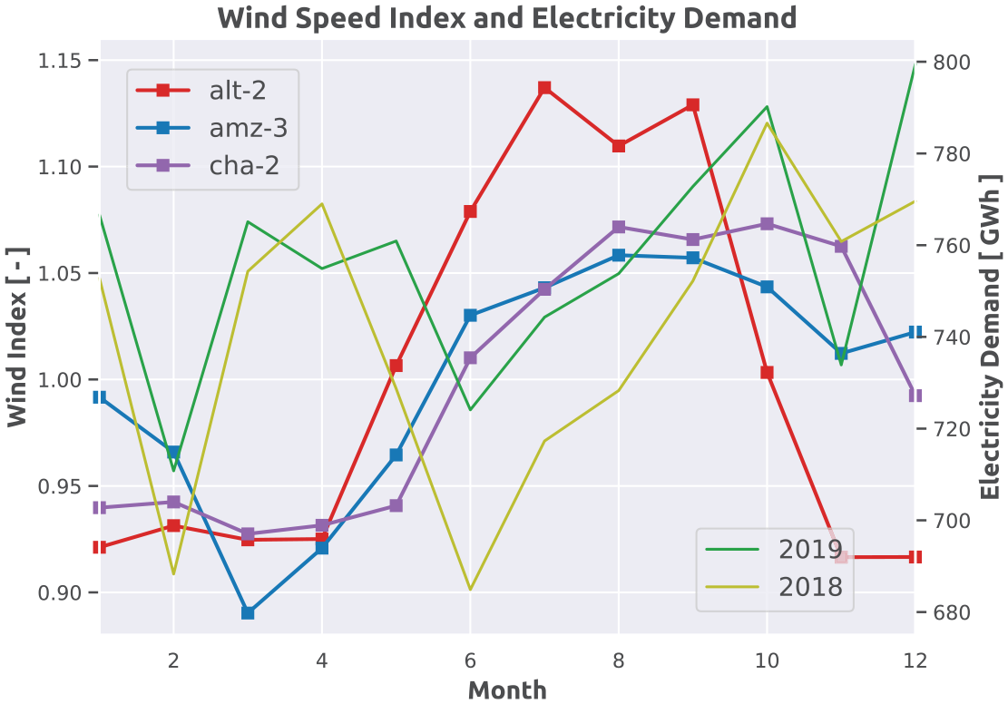
Wind speed index by month in three representatives sites. Altiplano (alt-2), Amazon (amz-3) and Chaco (cha-2) using MERRA-2. Second y-axis electricity demand (GWh) in the Bolivian interconnected system, 2018-2019. Data from CNDC (2010).

Table 3 shows the temperature and wind speed varibility over 41 years in the sites of study. The parameters of the regression are variation (slope) and T-0 and WS-0 are the values in 1980 (intercept). The variation in temperature are between 0.00054 and 0.0548°C yr ⁻¹. In function of the regions the mean decadal increment is 0.17, 0.225, and 0.406°C in the Altiplano, Amazon, and Chaco, respectively. However, the global mean decadal increment in the period 1980–2010 was 0.168°C (Vose et al., 2012) and in the Bolivian Amazon and Chaco increments are considerably higher than the global mean, and those reported by Aparicio-Effen et al. (2016) for the Bolivian Chaco.

Table 3.

Climate analysis in the different regions of Bolivia.

Regression values	alt-1	alt-2	alt-3	alt-4	amz-1	amz-2	amz-3	cha-1	cha-2
*Variation T [°C year⁻¹]	0.0171	0.0154	0.0162	0.0191	0.0057	0.0346	0.0272	0.0264	0.0548
**T-0 [°C]	7.19	7.62	14.74	6.89	26.26	24.81	23.78	22.59	15.51
r Value-T	0.518	0.454	0.615	0.559	0.122	0.596	0.518	0.575	0.826
*Variation WS [m/s year⁻¹]	−0.0011	−0.0011	−0.0022	0.0045	−0.0030	0.0028	0.0029	−0.0082	0.0042
**WS-0 [m/s]	4.26	4.55	4.76	4.78	3.73	3.47	6.56	6.93	3.87
r Value-WS	−0.12	−0.08	−0.13	0.20	−0.21	0.24	0.13	−0.36	0.49

Slope parameter of the linear regression.

Intercept parameter of the linear regression.

The increment/decrement of wind speed in the range 1980–2020 has no trend by reason of low correlation coefficients varies between 0.08 and 0.49. Additionally, the yearly variations are insignificant, for example there is a decadal increment in cha-2 of 0.045 m/s (cha-2) and a decadal decrement in amz-1 of 0.03 m/s. The increment/decrement and their correlation coefficients shown an unclear trend of the wind speed during the period 1980–2020.

Wind patterns along Bolivia

The previous Figure 2 and Table 2 showed some patterns about the wind speed in the different regions of Bolivia and their different variability. However, the mountainous interface between the Altiplano and the Amazon are closely linked, that is the reason alt-3 wind speed index follows the trends of the Amazon sites.

The monthly wind speed index (Figure 3) was computed using the 41 years of data from MERRA-2 taking into account the same three representative sites of the Figure 2. According the Figure 3 the periods of high wind speed are: May—October in the Altiplano (alt-2), June—January in the Amazon (amz-3), and June—December in the Chaco (cha-2). Although, in the Amazon and Chaco the high wind speed is distributed over 7 months, this is only 5% higher than the mean wind speed; in case of the Altiplano the high wind speed is over 6 months; however, this is 10—15% higher than the mean wind speed. Additionally, the increment of the wind speed compared with their minimum are 23% and 16% for Altiplano and Amazon, respectively. Also, the wind speed index is compared with the electricity demand (second y-axis) of the Bolivian interconnected system of 2018 and 2019. The electricity demand has maximum in March, April, November and December reaching demands between 770 and 800 GWh; and the minimum is 680 GWh during February and June. The increment of the electricity demand is followed by the increment of wind speed index since June. However, the period January–May, when the wind speed index is minimum, the electricity demand is regularly around 750 GWh and this low wind speed index could represent a problem under high wind energy penetration scenario.

The Figure 4 shows the Power Spectrum Density (PSD), also known as Van der Hoven spectrum of the wind. The PSD is a measure of the power of a oscillating variable in function of its frequency. In this case the variable is the wind speed and its variance is proportional to the kinetic energy of the wind speed fluctuation (Van der Hoven, 1957). Previous works (Escalante Soberanis and Merida, 2015; Harris, 2008) showed the importance of PSD for description of wind speed variability and identification of variation patterns in the frequency domain. The PSD of the Altiplano shows a strong peak at 1 day, weak peaks at 12 and 8 hours, and a concentration of different peaks after 5 days. The curve after 5 day correspond to the combination of mesoscale, global, and long-term wind speed variation into this is included the ENSO variability (Garreaud and Aceituno, 2001), that is known as synoptic variation (Van der Hoven, 1957). However, there is the diurnal variation and the 12 hours variations that is more related to the day-night cycle (Stull, 1988) due to the sunlight hours during the year have short difference between winter and summer.

Figure 4.

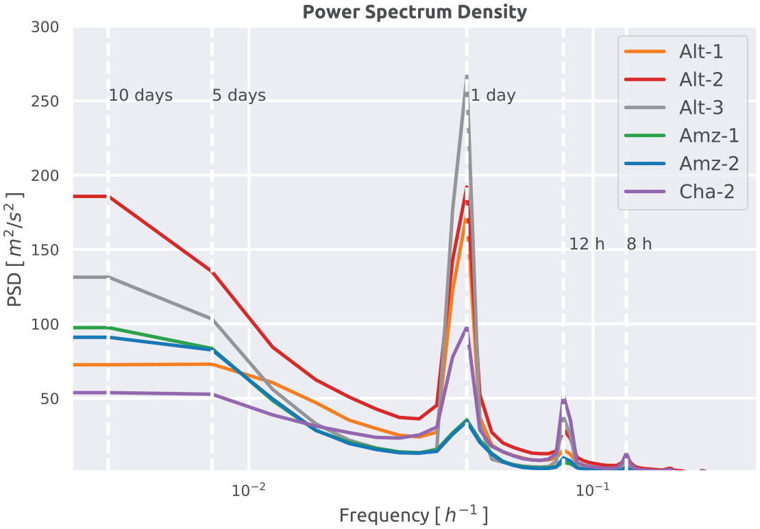
Power Spectral Density in different regions of Bolivia.

MERRA-2 and WRF are compared for the different seasons of the year and alt-2, alt3, amz-2 and cha-2 were selected due to their representativeness according region and terrain. The Andes has flat (alt-2) and mountainous (alt-3) regions, the Amazon is mostly flat and have high vegetation (amz-3) and the Chaco has flat and mountainous (cha-2) zones, cha-2 was selected because there is wind energy projects over there. Table 4 shows the monthly average wind speed from WRF and MERRA-2 and their respective difference. The results in March displays 2 m/s of difference between WRF and MERRA-2 in sites with complex terrain. The difference in amz-3 and alt-2 (both flat) is 1.1 and -0.18 m/s, respectively. However, the difference in alt-2 is minimum (0.18 m/s). The months with higher wind speed, June and September, show higher differences between WRF and MERRA-2 in all sites in study. In June the differences in complex and flat terrain reached 2.11 and 4.76 m/s, respectively. The higher differences are in June and September; the lower in March and December. These are due to: how MERRA-2 estimates the wind speed and the limited ground measurements in the region. The first option is related to MERRA-2 estimates the wind speed in function of cloud movement and June-September are dry periods and the clouds are scarce over the sites under study (McCarty et al., 2016). The second option is related how to improve MERRA-2 data, this consists in correlating MERRA-2 estimates with ground measurements and these are scarce in Bolivia.

Table 4.

Comparison of wind speed from MERRA-2 and WRF.

Site	MARCH			JUNE
	WRF	MERRA	DIFF	WRF	MERRA	DIFF
alt-2	4.20	4.38	−0.18	5.93	4.85	1.08
alt-3	6.70	4.57	2.12	9.38	4.62	4.76
amz-3	8.67	7.58	1.10	9.24	7.13	2.11
cha-2	5.92	3.78	2.15	8.28	3.83	4.45
Site	SEPTEMBER			DECEMBER
	WRF	MERRA	DIFF	WRF	MERRA	DIFF
alt-2	4.91	4.42	0.49	4.37	4.16	0.20
alt-3	9.15	5.53	3.62	7.44	4.92	2.52
amz-3	8.67	7.12	1.55	8.36	7.43	0.92
cha-2	7.02	4.19	2.82	5.99	4.36	1.63

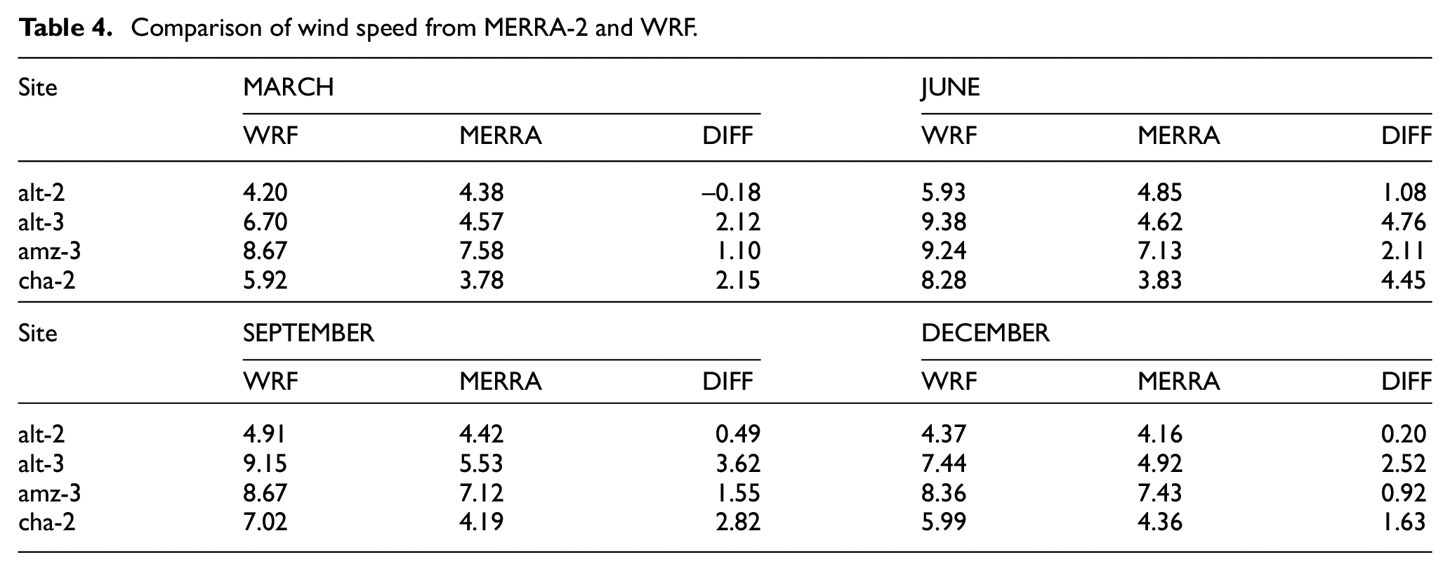
The results of WRF in alt-3 are closer to the measurements due to the wind speed average over there is 8 m/s (Mamani and Hendrick, 2019). However, the measurement is over a specific site and it is not over the grid size (30 km × 30 km). Clearly, WRF provides better estimates of wind speed closer to ground when the terrain is complex; however, the WRF results should be taken cautiously in complex terrain because the model is identifying the mountain winds and it is being extrapolated over all the grid when it occurs in specific sites.

In Figure 5, the wind speed of MERRA2 and WRF are compared in the sites discussed previously. The wind speeds in alt-2 show high variability and the WRF results following the trends of MERRA-2 data; however, there are days (17–27) with no relation between WRF and MERRA-2, although their mean wind speeds are similar. In amz-3 the wind speeds and trends are very similar with clear higher peaks simulated by WRF in the up-trend winds and that explains the 2.11 m/s higher mean wind speed showed by WRF (Table 4). The wind speeds in alt-3 show same trends with a notorious difference of 4 m/s (day 1–17 Figure 5); however, in the days 17–25 the similarities in magnitude between WRF and MERRA-2 are closer. The results in cha-2 show similar minimum winds with large differences in the maximum, these differences WRF and MERRA-2 reached 10 m/s. The wind speed simulated by WRF could be considered closer to the reality due to in cha-2 is being built a wind farm (Rojas Candia et al., 2019) and a mean wind speed of 3.83 m/s could be low for a wind farm project.

Figure 5.

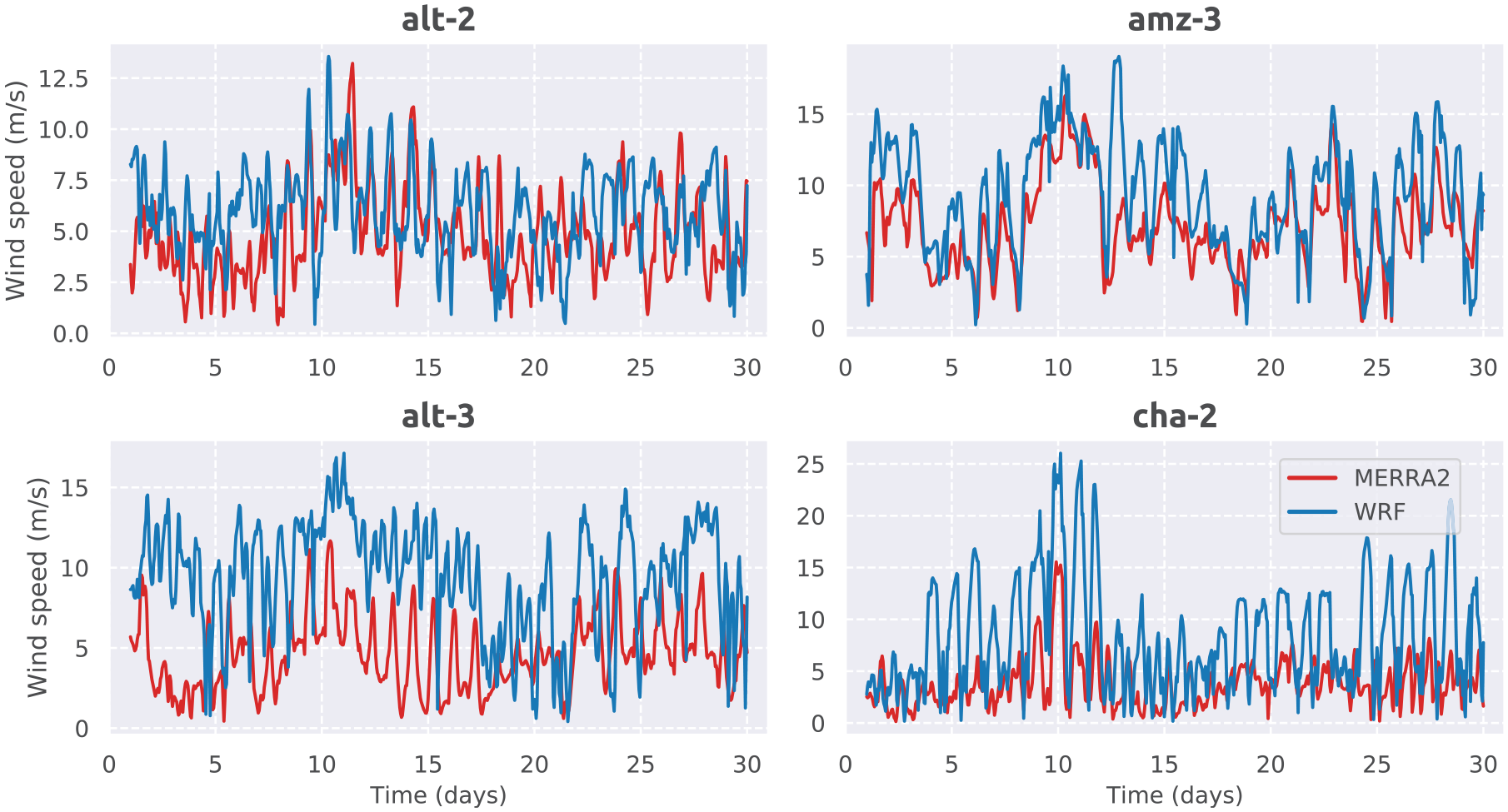
Comparison of wind speed between MERRA-2 and WRF.

The mean wind speed of a complete month and the average wind vectors are shown in the Figure 6, where each month represents a season: March (Autumn), June (Winter), September (Spring), and December (Summer). Most of the time the topographic characteristics define the wind characteristics and Bolivia topographically could be described as the Andes (Altiplano is included), the Amazon and the Chaco, those characteristics and their delimitation could be seen in Figure 1.

Figure 6.

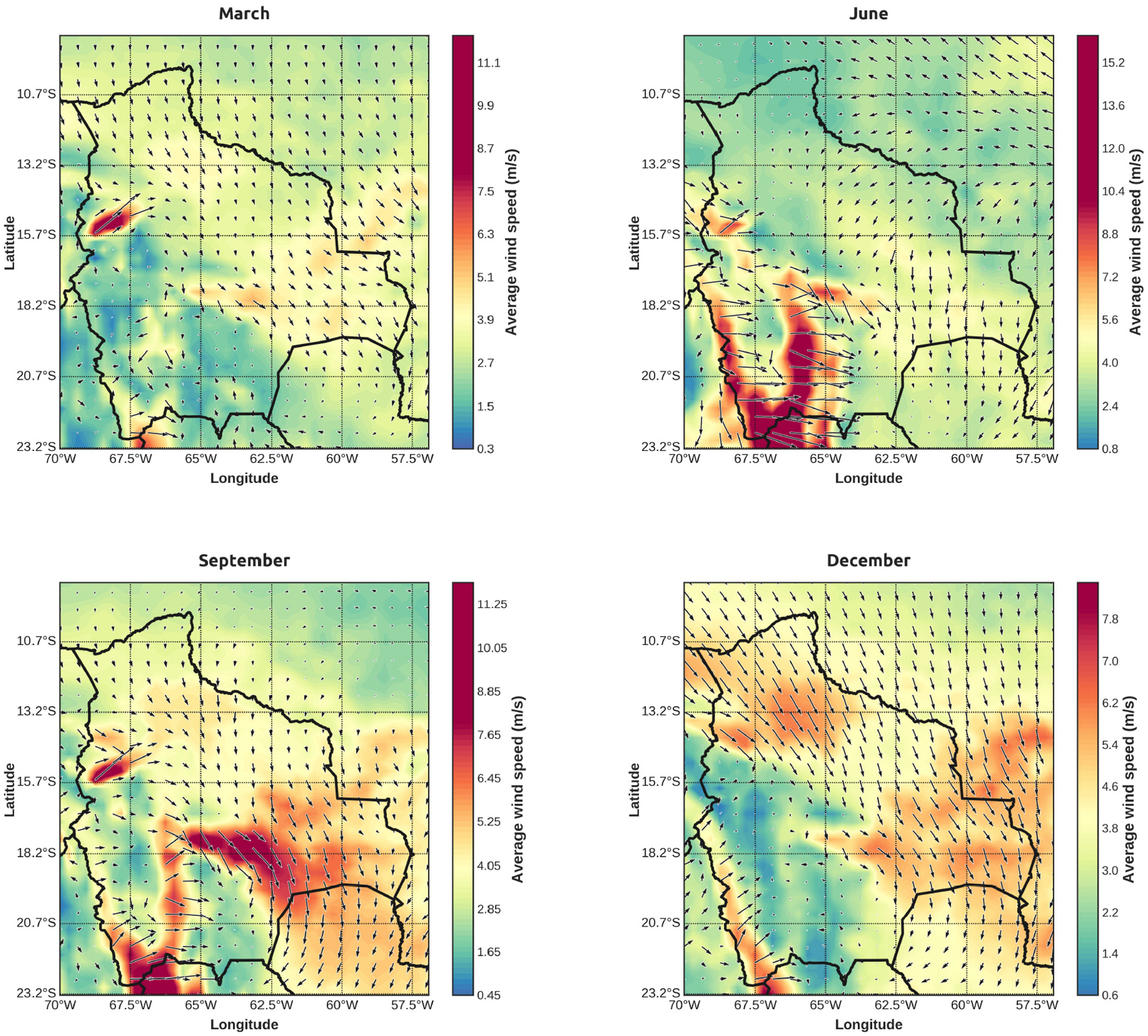
Wind vectors and mean wind speed of different seasons in Bolivia.

In March the mean wind speed reached 11 m/s and it was concentrated close to alt-1 (Andes) and there were wind speed of approximately 6 m/s over amz-2 and amz-3 regions (Amazon). The wind flow in the Amazon goes weakly from North to South, and in the Andes region is chaotic. During June the highest mean wind speed rises to 15 m/s and it is concentrated in the South region of the Bolivian Andes and with a defined wind flow, West to East. This wind characteristics over the southern Bolivian Andes coincide with the upper troposphere characteristics (Veblen et al. (2007); Garreaud et al. (2009); and the high wind speed could be due to up-slopes and down-slopes of the Andes coordillera (topographic conditions could be seen in the Figure 1) in combination with upper troposphere characteristics. In the Amazon region the wind flow is mostly from north to south in combination with the subtropical anticyclone (Veblen et al., 2007); because the anticyclone of the Atlantic generates the counter-clock wise wind flow (Insel et al., 2010).

In September and December the high wind speed is concentrated over Santa Cruz city (amz-3) with wind flows from north to south that follows the up-slopes of the eastern Andes coordillera and with maximum mean wind speed of 11 and 7.5 m/s, respectively. That wind flow produces a recirculating wind flow over the Bolivian Chaco (cha-1 and cha-2). However, the wind over the Andes in September and December have different characteristic. For example, during September the wind characteristic are similar to June; however, during December the wind speed is low and counter-clock wise flow patterns over alt-2; this because the subtropical anticyclone has as center the Bolivian Altiplano and this generates that pattern, as shown in Veblen et al. (2007) and Garreaud et al. (2009).

The Table 5 shows the wind shear of the different sites under study in this work. The region with lowest wind shear were the Andes and the Chaco; and the highest is over the Amazon. This wind shear characteristics are influenced by the the temperature, the surface type and for example, the wind shear for surfaces, such as grass and forest are 0.16 and 0.28, respectively (Emeis, 2013). The Andes and the Chaco are arid and their wind shear are close to 0.16. However, the Amazon is very known for their forests and their wind shear is proximate to 0.28, where amz-2 has the highest wind shear. An important region for wind energy generation is the Andes and there were measurement campaigns during 2013–2014 and some that data is used to compare the observed and WRF simulated wind shear. The observations were at alt-1 (Table 5) and the observed values are always smaller than WRF-simulated with relative errors between 0.5 % (March) and 26 % (September). These differences are mainly due to the gridding spacing in the simulation (30 km) because WRF averages the topographic and surface type of the grid in one single value, for this reason WRF overestimates the wind shear. Additionally, the high wind shear was during the June—September (cold period) and the low wind shear March—December (warm period) due to the wind shear is inversely proportional to temperature. The wind shear in alt-1 is higher for their land characteristics due to the way we computed the absolute value of the wind shear, because in alt-1 (observations and simulations) occurs negative values, which means occurs katabatic winds (Lopez and Howell, 1967).

Table 5.

Wind shear in the different regions of Bolivia.

Month	alt-1	alt-1 Obs	alt-2	alt-3	alt-4	amz-1	amz-2	amz-3	cha-1	cha-2
March	0.176	0.149	0.173	0.143	0.217	0.251	0.322	0.193	0.252	0.153
June	0.186	0.185	0.227	0.146	0.335	0.280	0.305	0.193	0.259	0.180
September	0.227	0.180	0.196	0.143	0.251	0.280	0.340	0.199	0.273	0.141
December	0.168	0.138	0.183	0.144	0.263	0.238	0.313	0.186	0.245	0.155

Conclusions

The wind characteristics in Bolivia for wind energy purposes are calculated and studied using the MERRA-2 dataset and simulations with WRF-ARW model. MERRA-2 was useful to describe the different long-term wind characteristics and WRF-ARW was useful to determine specific wind variation along different regions of Bolivia. The main results are related to wind speed index, wind variability, wind shear and wind speed differences between MERRA-2 and WRF-ARW. The wind speed indexes showed large differences and variability in alt-2 and amz-3 sites, where the maximum wind speed index reached 1.09 (alt-2) and the minimum 0.90 (amz-3). Also the results showed that Amazon wind has strong influence in the wind over the Andean mountains nearby. The MERRA-2 temperature data showed a mean decadal increment of 0.17°C (Altiplano), 0.225°C (Amazon), and 0.406°C (Chaco). In case of the wind the decadal variation showed no trend of increment/decrement over 41 years. The Altiplano showed higher differences between high and low wind along the year in comparison with the Amazon and Chaco. The periods of high wind speed are May—October in the Altiplano; and June—December in the Amazon, and Chaco. Finally, WRF tends to simulate larger wind speeds than MERRA-2, particularly in complex terrains where the difference reached 4.76 m/s.

This work explores additional sources of wind speed data for wind energy studies, such as wind energy projects, wind energy integration (interconnected system and microgrids) and energy balances in the interconnected system. Nowadays, the main region for wind energy projects is around Santa Cruz city (amz-3), due to its proximity to the biggest city in Bolivia. However, there is high wind energy potential in the Southern of the country (border with Argentina and Chile), which is associated with technical challenges, such as new transmission lines, and adequate wind turbines for high altitude conditions.

Footnotes

Copyright

Declaration of conflicting interests

The author(s) declared no potential conflicts of interest with respect to the research, authorship, and/or publication of this article.

Funding

The author(s) disclosed receipt of the following financial support for the research, authorship, and/or publication of this article: The authors would like to thank to Académie de Recherche et d’Enseignement Supérieur (ARES-CCD) for supporting this work, also we acknowledge to the NCAR Research Data Archive () that was esential for this work.

ORCID iD

Rober Mamani

References

3TIER (2009) Bolivia wind atlas: A project for the International Finance Corporation (IFC). Technical report, 3TIER.

Aldeman

Loomis

(2019) Wind energy production uncertainty associated with wind assessments of various intervals. Wind Engineering 44(4): 373–389.

Al-Yahyai

Charabi

Gastli

(2010) Review of the use of Numerical Weather Prediction (NWP) Models for wind energy assessment. Renewable and Sustainable Energy Reviews 14(9): 3192–3198.

Aparicio-Effen

Arana

Aparicio

, et al. (2016) Climate change and health vulnerability in Bolivian Chaco ecosystems. In: Leal Filho

Azeiteiro

Alves

(eds) Climate Change and Health: Improving Resilience and Reducing Risks. Cham: Springer International Publishing. pp.231–259.

Balderrama

Lombardi

Riva

, et al (2019) A two-stage linear programming optimization framework for isolated hybrid microgrids in a rural context: The case study of the El Espino community. Energy 188: 116073.

Bauer

Thorpe

Brunet

(2015) The quiet revolution of numerical weather prediction. Nature 525(7567): 47–55.

Canedo-Rosso

Hochrainer-Stigler

Pflug

, et al. (2019) Drought risk in the Bolivian Altiplano associated with El Niño Southern Oscillation using satellite imagery data. Natural Hazards and Earth System Sciences Discussions 2019: 21: 995–1010.

CNDC (2010) Comite Nacional de Despacho de Carga. Available at: https://www.cndc.bo/estadisticas/index.php (accessed 20 January 2021).

Emeis

(2013) Wind Energy Meteorology: Atmospheric Physics for Wind Power Generation. Springer. Berlin, Heidelberg.

10.

Escalante Soberanis

Merida

(2015) Regarding the influence of the Van der Hoven spectrum on wind energy applications in the meteorological mesoscale and microscale. Renewable Energy 81: 286–292.

11.

Franco

Gutierrez

Cataldo

(2020) An approach to model extreme wind speed distributions using the weather research and forecasting model. Wind Engineering 44(4): 341–360.

12.

García-Díez

Fernández

Fita

, et al. (2013) Seasonal dependence of WRF model biases and sensitivity to PBL schemes over Europe. Quarterly Journal of the Royal Meteorological Society 139(671): 501–514.

13.

Garreaud

Aceituno

(2001) Interannual rainfall variability over the South American Altiplano. Journal of Climate 14(12): 2779–2789.

14.

Garreaud

Vuille

Compagnucci

, et al (2009) Present-day South American climate. Palaeogeography, Palaeoclimatology, Palaeoecology 281(3): 180–195.

15.

Gelaro

McCarty

Suarez

, et al. (2017) The modern-era retrospective analysis for research and applications, version 2 (MERRA-2). Journal of Climate 30(14): 5419–5454.

16.

Gruber

Klckl

Regner

, et al. (2019) Assessing the Global Wind Atlas and local measurements for bias correction of wind power generation simulated from MERRA-2 in Brazil. Energy 189: 116212.

17.

Harris

(2008) The macrometeorological spectruma preliminary study. Journal of Wind Engineering and Industrial Aerodynamics 96(12): 2294–2307.

18.

Hodge

BMS

Ela

Milligan

(2012) Characterizing and modeling wind power forecast errors from operational systems for use in wind integration planning studies. Wind Engineering 36(5): 509–524.

19.

Hong

Noh

Dudhia

(2006) A new vertical diffusion package with an explicit treatment of entrainment processes. Monthly Weather Review 134(9): 2318–2341.

20.

Iacono

Delamere

Mlawer

, et al. (2008) Radiative forcing by long-lived greenhouse gases: Calculations with the AER radiative transfer models. Journal of Geophysical Research: Atmospheres 113(D13) 1–8.

21.

Insel

Poulsen

Ehlers

(2010) Influence of the Andes Mountains on South American moisture transport, convection, and precipitation. Climate Dynamics 35(7): 1477–1492.

22.

Lopez

Howell

(1967) Katabatic winds in the equatorial Andes. Journal of Atmospheric Sciences 24(1): 29–35.

23.

Mamani

Hackenberg

Hendrick

(2018) Efficiency of high altitude on-shore wind turbines: Air density and turbulence effects Qollpana wind farm (Bolivia). Proceedings 2(8): 487.

24.

Mamani

Hendrick

(2019) Wind farm power short-term prediction using WRF model and Kalman filtering. In: 32nd international conference on efficiency, cost, optimization, simulation and environmental impact of energy systems, Wroclaw, Poland, 23–28 June 2019. Institute of Thermal Technology - Gliwice

25.

McCarty

Coy

Gelaro

, et al. (2016) MERRA-2 input observations: Summary and assessment. NASA Tech Rep 46: 64.

26.

Null

(2000) El Niño and La Niña Years and Intensities Based on Oceanic Niño Index (ONI). Available at: https://ggweather.com/enso/oni.htm (accessed 20 January 2021).

27.

Olson

Kenyon

Djalalova

, et al. (2019) Improving wind energy forecasting through numerical weather prediction model development. Bulletin of the American Meteorological Society 100(11): 2201–2220.

28.

Penchah

Malakooti

(2020) The eastern-Iran wind-resource assessment through a planetary boundary layer simulation (2011–2015). Wind Engineering 44(3): 253–265.

29.

Perea-Moreno

Alcala

Hernandez-Escobedo

(2019) Seasonal wind energy characterization in the Gulf of Mexico. Energies 13(1): 93.

30.

Rabbani

Zeeshan

(2020) Exploring the suitability of MERRA-2 reanalysis data for wind energy estimation, analysis of wind characteristics and energy potential assessment for selected sites in Pakistan. Renewable Energy 154: 1240–1251.

31.

Rojas Candia

Balderrama Subieta

, et al. (2019) Techno-economic assessment of high variable renewable energy penetration in the Bolivian interconnected electric system. International Journal of Sustainable Energy Planning and Management 22: 17–38.

32.

Skamarock

Klemp

Dudhi

, et al. (2008) A description of the advanced research WRF version 3. Technical report, NCAR.

33.

Stull

(1988) An Introduction to Boundary Layer Meteorology. Dordrecht: Springer Netherlands.

34.

Thompson

Field

Rasmussen

, et al. (2008) Explicit forecasts of winter precipitation using an improved bulk microphysics scheme. Part II: Implementation of a new snow parameterization. Monthly Weather Review 136(12): 5095–5115.

35.

Van der Hoven

(1957) Power spectrum of horizontal wind speed in the frequency range from 0.0007 to 900 cycles per hour. Journal of Meteorology 14(2): 160–164.

36.

Veblen

Young

Orme

(2007) The Physical Geography of South America. Oxford Regional Environments. Oxford: Oxford University Press.

37.

Vose

Arndt

Banzon

, et al. (2012) NOAAs merged land ocean surface temperature analysis. Bulletin of the American Meteorological Society 93(11): 1677–1685.