Computational investigation of NREL Phase-VI rotor: Validation of test sequence-S measurements

Abstract

A CFD-based assessment and validation of the NREL Phase-VI Sequence-S rotor at seven wind speeds presented here. The ability of a three-dimensional, unstructured, unsteady RANS solver in successfully predicting the wind flow interactions with a rotating, twisted and tapered rotor is described. The uRANS equations were coupled with SST κ-ω turbulence model and a correlation-based Gamma-Theta transition model. The simulations were performed in ANSYS CFX using both Single Reference Frame (SRF) and Multiple Reference Frame (MRF) modelling approaches. A good agreement with measurements is observed at six of seven wind speeds when comparing the integral quantities, the spanwise and chordwise distributions. The only exception is the 10 m/s wind speed case, attributed to the onset of a massive leading edge stall around the mid-span region. It is successfully demonstrated here how uRANS-based CFD computations can be effectively employed in the study of wind turbine rotor aerodynamics.

Keywords

NREL Phase-VI rotor CFD wind turbine aerodynamics RANS S809 airfoil validation

Introduction

Wind energy is at a cusp, poised to revolutionize the energy sector by taking over the burden of continuing to propel the industrial revolution from fossil fuels (Gielen et al., 2018). The trend is unmistakably clear, as evidenced by the steady double-digit annual growth rates of wind power plant installations globally over the last two decades (GWEC, 2017). This momentum is predicted to continue well into the next decade with the successful commercialization of bigger and bigger wind turbines with lower energy production costs by several Original Equipment Manufacturers (OEMs) (Sadorsky, 2021). Such aggressive expansion necessitates optimizing the location of individual wind turbines inside a wind farm to maximize their collective Annual Energy Production (AEP) yield. It also calls for improvement in the existing wind turbine designs to maximize their Coefficient of Power (C_p), especially at all below-rated upstream conditions encountered by a wind turbine in a wind farm. A good understanding of the physics of lower atmospheric wind and wake flow evolutions in different terrains, combined with an ability to accurately predict the aeroelastic response of different turbine designs for various upstream conditions encountered in a wind farm, can help support this cause.

Wind turbine blades often operate in a dynamic environment subjected to ambient turbulence and gusts, resulting in unsteady flow over the entire rotor surface. The wind flow interactions with a turbine rotor is a complex non-linear process. Empirical and CFD models are developed to predict the resulting physical behaviour for various upstream conditions encountered in a wind farm. However, reliable measurements are needed as benchmarks to test and validate the accuracy of these models. One of the most crucial campaigns designed to provide reliable and comprehensive data to the wind turbine modelling community is the National Renewable Energy Laboratory’s (NREL) Phase-VI unsteady aerodynamic experiment (Hand et al., 2001). The NREL campaign was conducted at the National Aeronautics and Space Administration’s (NASA) Ames wind tunnel about two decades back. These measurements employed a two-bladed, stall-regulated and fully instrumented wind turbine having a rotor diameter of 10.058 m and a rated power capacity of 20 kW. The test turbine blades are twisted, tapered and designed exclusively using an S809 airfoil for which a well-documented wind tunnel database is readily available (Hand et al., 2001; Simms et al., 2001). Many measurements covering a wide range of operating conditions were performed as a part of this test campaign. The detailed specifications of the NREL wind turbine, including the various measurements performed with it, can be found in Hand et al. (2001). The data from these tests have proven to be a precious resource for the developers of wind turbine modelling tools (Simms et al., 2001). A validated wind turbine CFD model, in particular, is a handy tool for understanding the three-dimensional aerodynamic interactions and quickly evaluating the performance of various wind turbine rotor designs. The distinct advantage of CFD is its non-reliance on empirical inputs.

Simms et al. (2001) reported a comprehensive summary of the results of blind comparisons between different model predictions and NREL Phase-VI measurements. This exercise aims to benchmark the capabilities of the various wind turbine modelling tools by employing them to predict the output of selected phase-VI campaign cases. However, surprisingly this blind comparison exercise showed wide variations between predictions and measurement results. According to Simms et al. (2001), even the supposedly ‘easy to predict’ no-yaw, steady-state, 7 m/s wind speed case showed wide scatter in integral quantities like turbine power output and blade bending force. The predictions at higher wind speeds produced a 30% to 275% discrepancy compared to the corresponding experimental values when the turbine rotor blades are in a stall.

Sorenson et al. (2002) were among the first to apply the incompressible Reynolds Averaged Navier-Stokes (RANS) solver to simulate the NREL Phase-VI Sequence-S cases, which had an upwind rotor configuration with a yaw angle of 0°. The author performed a series of blind comparison studies to demonstrate the effectiveness of their in-house CFD code, called EllipSys3D, in predicting the performance of the two-bladed NREL wind turbine rotor at six different wind speeds. A good agreement was observed between the measurements and CFD computations in five of six test cases. The ‘10 m/s’ wind speed case was found to be an outlier as it showed significant deviations compared to the measurement results, which incidentally was attributed to the onset of massive flow separation along the span of the rotor blades resulting in a volatile aerodynamic behaviour. To avoid such substantial departures from measurements, the author suggested including transition models in future RANS simulations to more accurately capture the onset of rotor blade stall. Centrifugal forces influence the boundary layer evolution on the blades (Johansen and Sørensen, 2004; Sørensen et al., 2002), and the author presented limiting streamlines as proof to help visualize the radial flow enveloping a stalled rotor blade. Sorenson et al (2002) also stressed the need for 3D CFD computations to help better understand the three-dimensional effects of wind turbine flows.

Duque et al. (2003) employed a lifting-line code called CAMRAD II and a RANS code dubbed OVERFLOW-D to predict the aerodynamic performance of the NREL phase-VI two-bladed, horizontal axis wind turbine. The lifting line computations were performed for axial and yawed operating conditions, while the RANS simulations were conducted only for the axial cases. The authors noted that the OVERFLOW-D code could reliably predict the performance of a stalled rotor under various axial operating conditions. According to the authors, the Navier-Stokes method captures the post-stall behaviour quite well, thus providing a detailed insight into the fluid dynamics of the rotor blade stall. The OVERFLOW-D computations showed significant spanwise radial flow after the onset of the stall. Further, the authors’ analysis demonstrated that the lifting-line code required stall delay models to obtain the correct stall behaviour. However, even with these stall delay models, the lifting-line code still had difficulty in accurately predicting the power produced by a stalled wind turbine rotor.

Potsdam and Mavriplis (2009) relied on the Spalart-Allmaras turbulence model to perform CFD calculations on the NREL Phase-VI wind turbine rotor. The domain was discretized using an unstructured mesh with an adaptive grid refinement technique employed primarily to resolve the tip vortex evolution downstream in the near-wake region. The authors concluded that the results obtained from their unstructured grid solver, NSU3D, agree closely with those obtained from the well-validated structured grid solver, OVERFLOW, but noted that the node count would be larger with the former. Oscillations were reported on the rotor surface static pressure calculated with this unstructured grid solver methodology. Also, the authors performed simulations with both steady and unsteady formulations and reported similar performance predictions using both these approaches. The steady formulation was observed to be computationally more efficient. However, the authors argued that the unsteady formulation helps in modelling the effects of a ground plane, non-uniform inflow, nacelle, and tower.

Gerber et al. (2005) employed the NREL’s Lifting Surface Prescribed Wake code (LSWT) to analyse the performance characteristics of various rotor segments along the span of NREL phase-VI rotor, focussing primarily on the peak and post-peak rotor aerodynamics. The lift and drag coefficients at different radial positions were obtained through an iterative process using the angle of attack distribution predicted by the LSWT and the measured normal and tangential force coefficients. According to the authors, the peak and post-peak power predictions are influenced by five significant aerodynamic events, which must be taken into account by the wind turbine model developers. A stall delay was observed at 30% and 47% blade span just before the peak power, which enhanced the measured power production beyond those predicted using the 2D airfoil data. More importantly, the authors noted a rapid increase in the drag at 47% span as soon as the turbine reaches its peak operating capacity. The authors argued that this drag increase governs the wind turbine’s peak power production. Similar to other studies, they reported total flow separation in the post-peak power region at the highest tested wind speed. The flow separation starts near the blade root at peak power and then moves towards the blade tip region as the wind speed increases, eventually engulfing the whole blade.

Yelmule and Vsj (2013) demonstrated the capabilities of CFD simulations in predicting the complex three-dimensional aerodynamics of the NREL Phase-VI rotor using a Gamma-Theta transition model. The authors validated their CFD computations with NREL Test Sequence-S measurements, which had an upwind rotor configuration with 0° yaw and 3° blade tip pitch angle. The domain was discretized using a structured mesh, and several steady-state simulations were performed using the multi-purpose ANSYS CFX solver. Six of seven test cases reported excellent qualitative and quantitative agreement with measurements. The test case with an input upstream wind speed of 10 m/s was identified as an exception attributed to the onset of the stall. At low wind speeds, say 7 m/s, the flow is found to be nicely attached to the blade surface everywhere along its length except in the region below 30% span. Also, the transition is observed close to mid-chord, as evidenced by the limiting streamlines. During the onset of the stall at 10 m/s, the flow separation starts near the leading edge around the mid-span location. The stall, thus initiated at mid-span, begins to move over the entire blade as the wind speed increases, eventually disrupting the flow over the complete rotor. Yelmule and Vsj (2013) concluded that steady-state CFD computations predict integrated quantities like power and thrust within the measurement uncertainty. However, quantitative differences are observed in pressure distribution on the suction side due to the specific stall behaviour of the S809 airfoil. The CFD simulations also had difficulty capturing the large transient effects occurring at the onset of the stall.

Zhong et al. (2018) demonstrated that the accuracy of RANS-based predictions of the NREL Phase-VI rotor could be significantly improved by calibrating the rotor simulations with the experimental data available for the S809 airfoil. The authors argued that the primary reason for discrepancy is not the 3-D rotational effects but a significant overestimation of the aerodynamic lift forces for the S809 airfoil at the onset of the stall. Further, the authors claimed that the lift coefficients are underestimated in the deep stall region. The discrepancy in rotor simulations shows a high degree of similarity with the corresponding error in airfoil simulations. This discrepancy is greatly reduced by tweaking one of the turbulence closure coefficients in the SST turbulence model. They identified the turbulence closure coefficient that has the most significant impact on the stall predictions in both airfoils and rotors. The error in their RANS-based NREL Phase-VI rotor predictions at all wind speeds is largely reduced when the value of this coefficient is adjusted to match well with the S809 airfoil lift characteristics.

The CFD simulations of the NREL Phase-VI Sequence-S measurement cases were also reported by Song and Perot (2015). The surface pressure distributions and bulk quantities like shaft torque were predicted at seven different ambient upstream wind speeds. Their simulations showed reasonable agreement with experimental values for inlet wind speeds lower than ‘10 m/s’ when the flow is still attached to the blades. However, significant differences between CFD predictions and measurements were observed at all higher wind speeds. The authors attributed those differences to the three-dimensional nature of the separated flow field over the blades and to the turbulence model employed in their calculations. The sensitivity of grid resolution on the resulting accuracy of their CFD predictions is also discussed.

A summary of the NREL Phase-VI CFD model validation case studies reported in the open literature is presented in Table 1. The current work is also included in Table 1 to compare and benchmark it against past studies. In almost all the works discussed above, the authors used 180° periodicity to simulate only one blade. Suppose one assumes the wind turbine rotor blades and tower as stiff members, which is a fair assumption, especially for such a small kW-sized wind turbine (Hand et al., 2001; Simms et al., 2001). Then the aerodynamic response of such a wind turbine’s rotor to different upstream wind conditions is primarily governed by its outer geometry.

Table 1.

Summary of NREL Phase VI CFD model validation cases addressed in the literature.

Reported by	Turbine Geometry	Mesh type	Mesh count	First cell thickness (microns)	Solver	Approach	Turbulence model	Transition model	Wind speeds (m/s)
Duque et al. (2003)	Both rotor blades and hub	Structured grid	~13 million nodes	50	OVERFLOW-D, CAMRAD-II	RANS, Lifting- line	Baldwin-Barth, Free wake model	Beddoes-Leishman dynamic stall model	7, 10, 13, 15, 20, 25
Song and Perot (2015)	Both rotor blades	Unstructured grid	10 million elements	50	OpenFOAM 1.6-ext	RANS	Spalart-Allmaras (S-A)	None	5, 10, 25
Yelmule and Vsj (2013)	One rotor blade with spherical hub. Tunnel walls not considered.	Structured grid	–^a	– ^a	ANSYS CFX 12.1	Unsteady RANS	k- $ω$ SST	Gamma -Theta	5, 7, 10, 13, 15, 20, 25
Potsdam and Mavriplis (2009)	Isolated rotor	Structured grid	8.6 million nodes & 15.7 million nodes	6	NSU3D OVERFLOW-D OVERFLOW-3	RANS	S-A Model, Baldwin-Barth	None	7, 10, 15, 25
Mo and Lee (2012).	Single blade	Structured grid	3 million cells	– ^a	ANSYS FLUENT	RANS	k- $ω$ SST	– ^a	– ^a
Xu and Sankar (2000).	Single blade	Structured	– ^a	– ^a	ln-house code	RANS	Baldwin-Lomax	None	10, 15, 20
Lanzafame et al. (2013)	Both rotor blades	Unstructured grid	9 million polyhedral cells	– ^a	ANSYS FLUENT 13	RANS	Transitional SST	– ^a	– ^a
Sorenson et al (2002).	One rotor blade with spherical hub. With and without tunnel	Structured grid	3.1 & 42 million cells	– ^a	EllipSys3D	RANS	k- $ω$ SST	None	7, 10, 13, 15, 20, 25
Current work	One rotor blade only. Tunnel walls not considered	Unstructured grid	19.4 million nodes & 46.6 million elements	3.75	ANSYS CFX 2021 Rl	RANS	k- $ω$ SST	Gamma -Theta	5, 7, 10, 13, 15, 20, 25

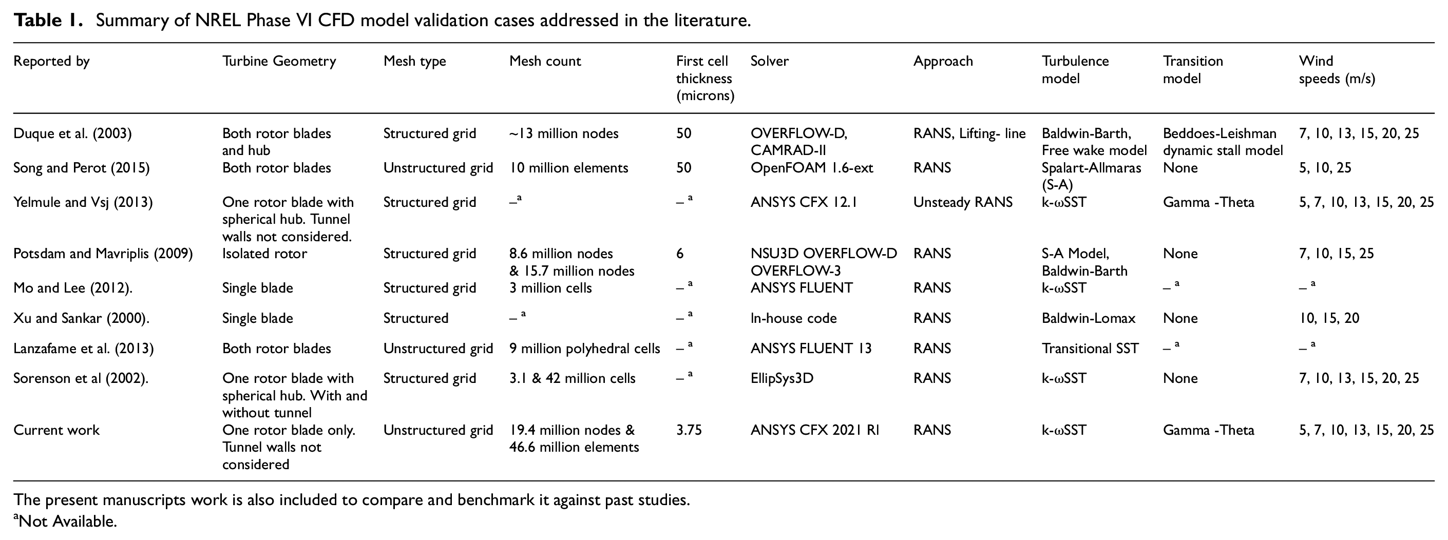
The present manuscripts work is also included to compare and benchmark it against past studies.

Not Available.

The manuscript presents comprehensive validation of unsteady RANS-based CFD computations of the NREL Test Sequence-S cases. The primary objective of the current work is to develop a validated CFD model of a two-bladed rotor using both SRF and MRF approaches. This validated model will then be employed to understand and evaluate the effects of minor design changes (e.g. a modified tip design or inclusion of vortex generators (Zhu et al., 2021)) on a wind turbine’s performance, to evaluate the performance of diffuser-augmented wind turbines (Ohya and Karasudani, 2010; Ohya et al., 2017), and also in other wind farm-level studies. We decided to validate our CFD methodology with a two- and a three-bladed wind turbine. Thus, NREL and MEXICO (Schepers et al., 2014) rotors were chosen as validation case studies for the two- and three-bladed wind turbines, respectively. The validated CFD approach developed here will also be employed to benchmark the drone-based wind measurement system (Subramanian et al., 2015) that is under development at IIT Tirupati.

NREL Phase VI Unsteady Aerodynamic Experiment

The NREL Phase-VI Unsteady Aerodynamics Experiment (UAE) is an excellent validation platform for testing and benchmarking the various wind turbine CFD models and other wind turbine modelling codes (Simms et al., 2001). These measurements provide an opportunity to understand the effects of wind flow interactions with a two-bladed turbine operating in a controlled environment. The measurement campaign was performed in the NASA Ames wind tunnel boasting a test section size of 24.4 m ×36.6 m. The test campaign employed a fully instrumented, stall-regulated horizontal-axis wind turbine having a rotor diameter of 10.058 m and a power rating of 20 kW. Its twisted-tapered blades were designed from a 25% span onwards using an S809 airfoil, whose geometry and aerodynamic characteristics are well documented in the open literature (Hand et al., 2001). The blade root is cylindrical, and a transition piece connects the circular cross-section with the airfoil cross-section. The complete blade geometry is provided in Hand et al. (2001).

The validation data set employed here is from Test Sequence-S, in which measurements were performed using a rigid wind turbine operating in an upwind configuration with no yaw misalignment, having a cone angle of 0° and a constant blade tip pitch angle of 3°. The upstream wind speeds ranged from 5 to 25 m/s. At all tested wind speeds, the rotor was rotated counterclockwise (when viewed from upstream) with a constant speed of 72.1 rpm. The Sequence-S measurements were performed with smooth, clean blades on which the boundary layer was allowed to transition freely (i.e. no zigzag roughness strips were put on the pressure and/or suction sides of the rotor blades). The aerodynamic forces and moments acting on the wind turbine rotor at different operating conditions were carefully measured and documented. The Sequence-S measurements include blade pressures, shaft torque, integrated and sectional aerodynamic loads, sectional inflow conditions, blade root strain and tip acceleration. According to Hand et al. (2001), the data measured in the NREL phase-VI experiment ‘can be considered highly accurate and reliable’; hence no further post-processing was performed on the measurement data. Also, the effects of blockage on measurement results can be considered negligible, as reported by Hand et al. (2001). A detailed description of the NREL phase-VI UAE can be found in Hand et al. (2001).

Computational setup

The validation is performed by comparing the integral, spanwise and chordwise distributions of rotor surface static pressure and loads calculated from CFD simulations with the corresponding values obtained from the NREL Sequence-S measurements. Commercial CFD solvers, like ANSYS CFX, have substantially improved their capabilities in the last two decades to become fast, accurate and reliable tools for solving engineering problems. One of the main reasons for this success is the advent of High-Performance Computing (HPC) clusters. The simulations reported here were executed in the ANSYS CFX 2021 R1 (ANSYS, Inc, 2021a, 2021b) using HPC to understand the physics of turbulent flow interactions with a rotating wind turbine rotor. An integrated package in the ANSYS workbench, called ICEM-CFD (ANSYS, Inc, 2021e), was utilized for meshing. As the underlying physical phenomena are complex and non-linear, the analysis reported here employs the unsteady Reynolds Averaged Navier-Stokes (uRANS) equations coupled with the Shear Stress Transport (SST) κ-ω turbulence model (Menter, 1994). The κ−ω SST turbulence model (Menter, 1993; Wilcox, 1991) is based on two transport equations: one for the turbulent kinetic energy κ and the other for specific turbulent dissipation rate ω, and is known to be very accurate in solving the flow field near wall regions (Zhang et al., 2017). Sørensen (2008) argued that the difference between the performance predictions obtained from transitional and fully turbulent simulations is small for the S809 airfoil; thus, reasonably accurate CFD computations can be performed with the NREL rotor geometry even by assuming the flow as a fully turbulent one. This claim is tested here by including a correlation-based Gamma-Theta transition model to control the laminar-turbulent transition process in the boundary layer (Eleni et al., 2012). The resulting partial differential equations were discretized and solved with a second-order accurate scheme using a finite volume-based CFX solver.

The uRANS based unsteady partial differential equations are shown below.

\frac{\partial ρ}{\partial t} + \frac{\partial}{\partial x_{i}} (ρ u_{i}) = 0

(1)

\begin{matrix} \frac{\partial}{\partial t} (ρ u_{i}) + \frac{\partial}{\partial x_{j}} (ρ u_{i} u_{j}) = - \frac{\partial p}{\partial x_{i}} + \frac{\partial}{\partial x_{j}} [μ (\frac{\partial u_{i}}{\partial x_{j}} + \frac{\partial u_{j}}{\partial x_{i}} - \frac{2}{3} δ_{ij} \frac{\partial u_{i}}{\partial xj})] \\ + \frac{\partial}{\partial x_{j}} (- ρ \bar{u_{i} u_{j}}) \end{matrix}

(2)

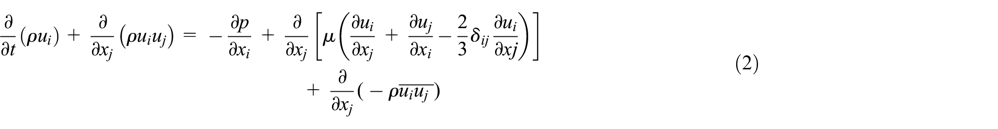
The Reynolds stress term $\bar{u_{i} u_{j}}$ is resolved according to the chosen turbulence model. An eddy viscosity-based turbulence model is chosen here to provide closure for the uRANS equations. At higher wind speeds, when the blade is in a stall or in a deep stall, random oscillations were observed in the CFD-predicted integral quantities like power and thrust. The numerical results presented here are time-averaged values of the last 10 rotor revolutions. The turbulent fluctuations are time-averaged in the RANS approach; thus, the mean flow properties can be accurately predicted. However, these equations must be solved in a moving frame of reference to capture the flow field around a rotating wind turbine blade accurately. Thus, the simulations presented here were performed using two different moving reference frame modelling approaches, Single Reference Frame (SRF) and Multiple Reference Frame (MRF). Both approaches are made possible by taking advantage of the constant rotational speed of the turbine rotor. The relative velocity formulation for the momentum conservation equation contains two additional terms to account for the coriolis and centripetal accelerations. In the case of SRF, the governing equations are solved in a rotating (inertial) frame of reference over the entire computational domain. In contrast, the governing equations in the MRF approach (also known as the frozen rotor approach) are solved in a rotating (inertial) frame of reference only inside a small inner domain containing the rotor. In the MRF approach, this small inner domain containing the rotor is rotated at a constant speed, while the large outer domain surrounding it is stationary relative to the ground. More details on these two moving reference frame modelling approaches can be found in ANSYS, Inc (2021c). The numerical investigation presented here assumes the flow field to be unsteady, compressible, and isothermal.

The computational domains employed in the SRF and MRF simulations are shown in Figure 1. A CAD model of the rotor blade was developed in-house from scratch using the details provided in Hand et al. (2001). The blade and the domain boundaries were modelled in CREO with a tolerance of 10^-8 m, then imported into ICEM-CFD for meshing. The original S809 airfoil has a very sharp trailing edge, but it is truncated at 98% chord length to produce a blunt edge along the entire blade span. The authors sincerely thank Mr. Lee Jay Fingersh from NREL for sharing the original CAD model of the test turbine’s blade tip. The terminologies used for the domain boundaries are shown in Figure 1. The inlet and outlet are located at a distance of four- and sixteen-rotor diameters from the rotor plane, respectively. At the same time, the cylindrical ‘tunnel wall’ boundary is placed at a distance of three rotor radius from the axis of rotation. The outer boundaries of the computational domain are identical in both SRF and MRF simulations. However, the only difference in the MRF model is the presence of a separate small half-cylindrical inner domain surrounding the blade, Figure 1. This inner domain’s semi-circular plane and curved boundary surfaces are positioned at a minimum distance of 2.5 m from the surface of the rotor blade.

Figure 1.

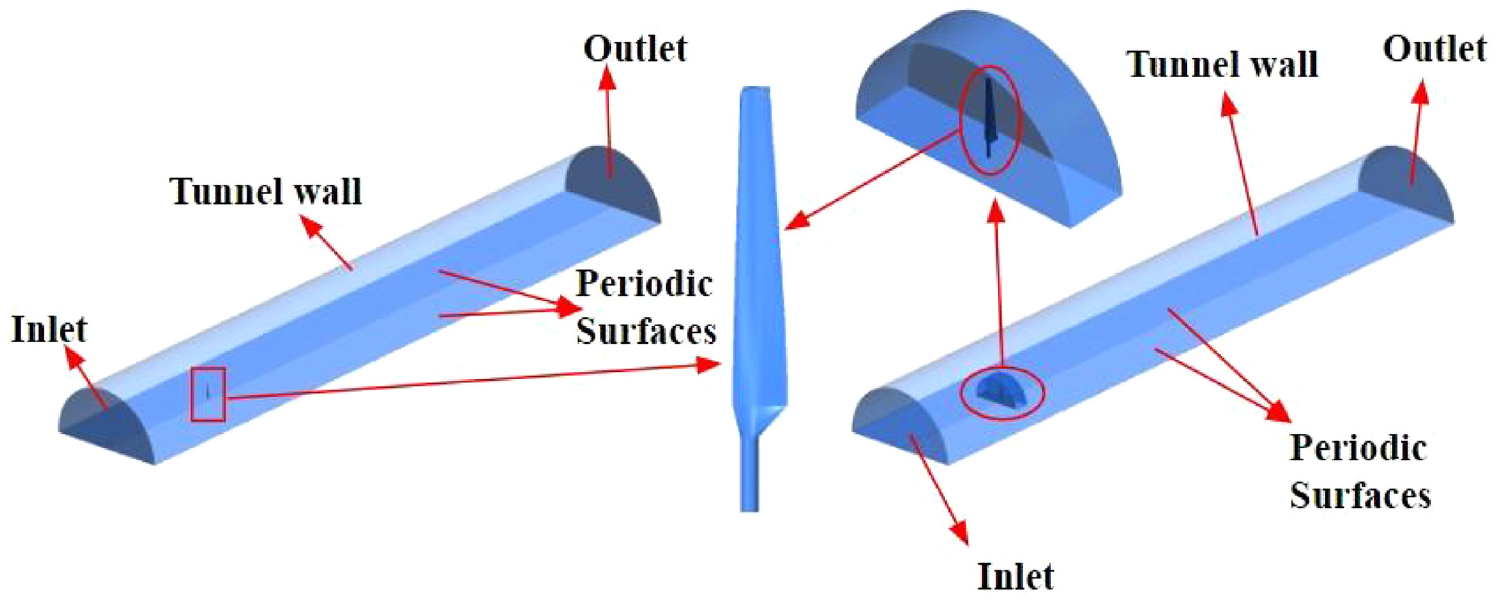
Computational domain: SRF (left) and MRF (right).

A good quality unstructured mesh is generated in ICEM CFD to facilitate the study of boundary layer growth over the blade surfaces. Sorenson et al (2002) reported that the stagnation point at any spanwise section is expected to lie near the leading edge on the pressure side of the rotor blade. Thus, the mesh near the leading edge along the entire blade span is resolved finely (both on the surface and in the direction normal to the surface) to capture the flow field in that region accurately, Figure 2. Similarly, the mesh is finely resolved around the trailing edge region along the entire blade span. The mesh on the blade surface at all spanwise locations covering r/R > 0.2 is refined sufficiently in the chordwise direction to have more than 300 nodes. Enhanced wall treatment requires the first cell centroid near the wall to be located within the viscous sublayer.

Figure 2.

Computational mesh in the vicinity of the rotor blade: Surface mesh on suction side (top), Mesh cut-plane at section A (bottom).

The first cell prism layer height is maintained at 3.75 microns over the entire blade surface to achieve a y⁺<1 everywhere on the rotor surface, which helps resolve the viscous sublayer directly. A total of 48 prism layers with a maximum growth rate of 1.2 is generated around the blade surface to accurately capture the gradients inside the boundary layer. The total extent of the inflation layers at any span location is dependent on the local chord (ANSYS, Inc, 2021d), and hence it varies continuously along the length of the blade. Similarly, the total extent of the inflation layers varies smoothly along the chordwise direction, as shown in Figure 2. These prism layers help accurately model the wall-bounded turbulence caused by the rotor blades.

A detailed mesh refinement study was performed to find the optimum mesh count that produces results independent of the grid resolution. Grid independence study was carried out using four different mesh counts −∼9 million (‘coarse’), ∼17 million (‘medium’), ∼38 million (‘fine’) and ∼68 million nodes (‘very fine’) – to find the optimum mesh size that is still fine enough to discretize the geometry. The mesh is coarsened (or refined) only near the blade surface but is kept nearly the same at all the other locations. These simulations were performed with inlet wind speeds of 10, 15.1 and 25.1 m/s. The integral quantities like power and thrust obtained at all three wind speeds (not shown here) clearly show that the difference between ‘fine’ and ‘very fine’ cases is less than 1%. Also, the spanwise sectional pressure distribution obtained using all four grid levels at the three wind speeds shows similar behaviour between the ‘fine’ and ‘very fine’ mesh cases. Therefore, the ‘fine’ mesh with ∼38 million nodes is considered sufficient, and all the results presented in this manuscript are obtained using it.

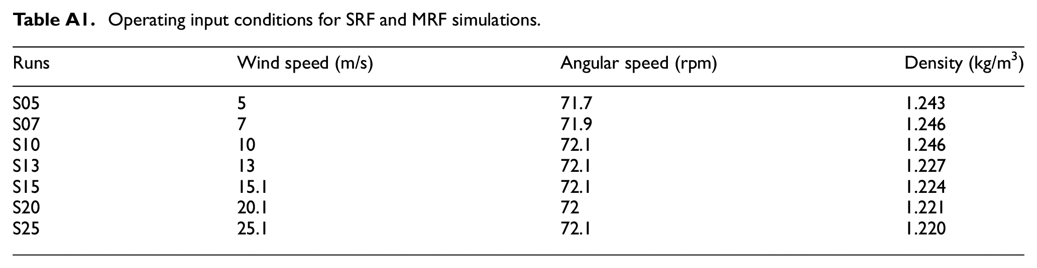
The boundary conditions employed in the stationary frame of reference can be summarized as follows. The inflow properties from NREL measurements (Hand et al., 2001) are supplied as input in the CFD analyses, Table A1 (in Appendix). The air flowing into the domain from the inlet boundary is assumed to be uniform with an isotropic turbulence intensity of less than 1%. The interference due to tunnel wall effects and blockage effects on the flow field around the test wind turbine is assumed to be negligible and thus not included in the CFD simulations. It is a valid assumption, as demonstrated by Sorenson et al (2002). Therefore, in all the SRF-based CFD calculations presented here, the rotor is assumed to operate in an undisturbed environment with an identical boundary condition specified at the inlet and tunnel wall boundaries. All MRF simulations employ a slip wall condition on the tunnel wall boundary. The relative gauge pressure is set to zero at the domain outlet. The blade surface is assumed to be smooth, with a no-slip boundary condition enforced on it. A periodic mesh is generated on the two periodic boundary surfaces, and a periodic boundary condition is provided here. In the case of MRF, the inner and outer domains are connected through a Generalized Grid Interface (GGI). The convergence is monitored by tracking scaled residuals in each iteration, which measures the overall conservation of the flow properties (Taylor, 1997). A numerical solution is considered fully converged once all the residuals and monitor points show a stabilized behaviour for more than 10 rotor revolutions.

Computational investigation with three-dimensional CFD simulations are valuable but remain very time-consuming. The nacelle, tower and hub are not included in our simulations as their influence on the results presented here is considered to be negligible (Song and Perot, 2015; Sørensen et al., 2002; Yelmule and Vsj, 2013). This assumption helps simplify the geometrical complexity of the problem as the modeller can take advantage of the 180° periodicity to model just one-half of the rotor domain containing only one blade, Figure 1. This simplification helps to reduce the computational efforts involved with each simulation. Though only half of the rotor geometry was employed, each simulation took ∼40 hours to complete on an HPC cluster with 64 processors. A total of ∼40 such simulations were performed as a part of the study reported here.

Results and discussions

Integrated quantities

The results obtained from CFD simulations are compared with the data collected by NREL during phase-VI Sequence-S measurements at the NASA Ames wind tunnel. A comparison between the integrated quantities like power, thrust, root flap and root edge moments obtained from measurements with the corresponding time-averaged values predicted by CFD using the SRF and MRF modelling approaches at seven different upstream wind speeds, is shown in Figures 3 and 4. The integrated quantities can be obtained from CFD computations by integrating the local values of static pressure and skin friction acting at all discretized points over the blade surface. The actual experimental values are shown using the best estimate (which is calculated by averaging the data collected over several rotor revolutions (Simms et al., 2001; Taylor, 1997)) along with error bars representing uncertainty of ±1σ in the best estimate (Taylor, 1997). The experimental values are represented using black colour markers, while the CFD results obtained from SRF and MRF modelling approaches are shown using red and green colour markers, respectively. An identical colour trend line is employed to connect all markers of the same colour.

Figure 3.

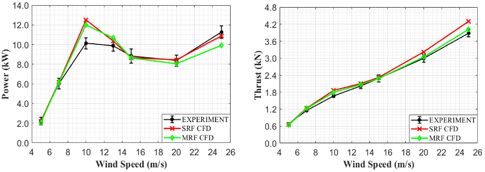
Comparison of power (left) and thrust (right) obtained from NREL Sequence-S measurements versus the corresponding time-averaged values predicted by CFD using the SRF and MRF models at seven different wind speeds. The measurement uncertainty is shown using ±1σ.

Figure 4.

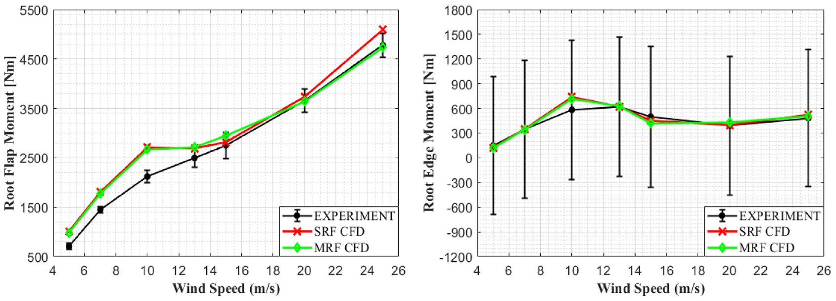
Comparison of blade root flap (left) and edge (right) moments obtained from NREL measurements versus the corresponding time- averaged values predicted by CFD using the SRF and MRF models at seven different wind speeds. The measurement uncertainty is shown using ±1σ.

As seen in Figure 3, there is a good quantitative agreement between CFD predictions and measurements at all wind speeds except for the 10 m/s wind speed case. At 10 m/s, there is an over prediction in power of ∼25% with SRF, and a corresponding over prediction in power of ∼20% with MRF, respectively. The observed difference between CFD predictions and measurements at 10 m/s is attributed to the onset of stall, when flow separation starts to cover the blade. Though a transition model is included in both SRF and MRF simulations to correctly predict the boundary layer transition, it still fails to bridge the gap between measurements and CFD predictions even for the integral quantities. The reason could be attributed to the sensitive nature of the transition process to even small disturbances occurring inside the wind tunnel test section. Nevertheless, these CFD predictions are still in good agreement with what other researchers had reported earlier (Duque et al., 2003; Mo and Lee, 2012; Song and Perot, 2015; Sørensen et al., 2002; Xu and Sankar, 2000; Yelmule and Vsj, 2013; Zhong et al., 2018; Zhou, 2017). At 25.1 m/s, there is a slight under prediction in power and an over prediction in thrust obtained from both SRF and MRF. The rotor is in a deep stall at this highest wind speed (e.g. see limiting streamlines in Figure 14).

As seen in Figures 3 and 4, the difference between MRF and SRF predictions is substantial even for the integral quantities at wind speeds of 10 m/s and higher. However, in the majority of cases, the deviations observed between SRF and MRF predictions compared to measurements is less than ±1σ. Similarly, there is a good qualitative and quantitative agreement between the computed and measured root flap and root edge moments, Figure 4. The large standard deviations in the case of root edge moment is due to the influence of gravitational loads during rotor rotation. Again, the difference between MRF and SRF predictions compared to measurements is more pronounced at 10 m/s. The SRF predictions result in a slightly better agreement with measurements compared to those obtained from MRF. For example, the deviations in captured power between SRF predictions and experimental values are less than the uncertainty in measurements at all wind speeds except at 10 m/s. The overall qualitative trend appears to be nicely captured using both SRF and MRF modelling approaches.

Spanwise variation of force and pressure coefficients

The spanwise distribution of the time-averaged normal (C_N) and tangential (C_T) force coefficients predicted through CFD calculations using SRF and MRF modelling approaches compared to the experimental values at seven different upstream wind speeds is shown in Figure 5. The uncertainty in the measurement values is shown in Figure 5 using plus/minus one standard deviation. For a given wind speed case, the experimental values of the force coefficients, C_N and C_T, at any of the five stations along the blade span are obtained from the surface static pressure measurements assuming a linear variation between any two adjacent pressure taps. Thus, the five different spanwise stations in Figure 5 are the locations (i.e. r/R = 0.3, 0.467, 0.633, 0.8 and 0.95) at which the surface static pressure measurements were performed. CFD predictions of the force coefficients at any section are computed from the SRF and MRF simulations using the formula suggested in Bechmann et al. (2011); Sørensen et al. (2002).

Figure 5.

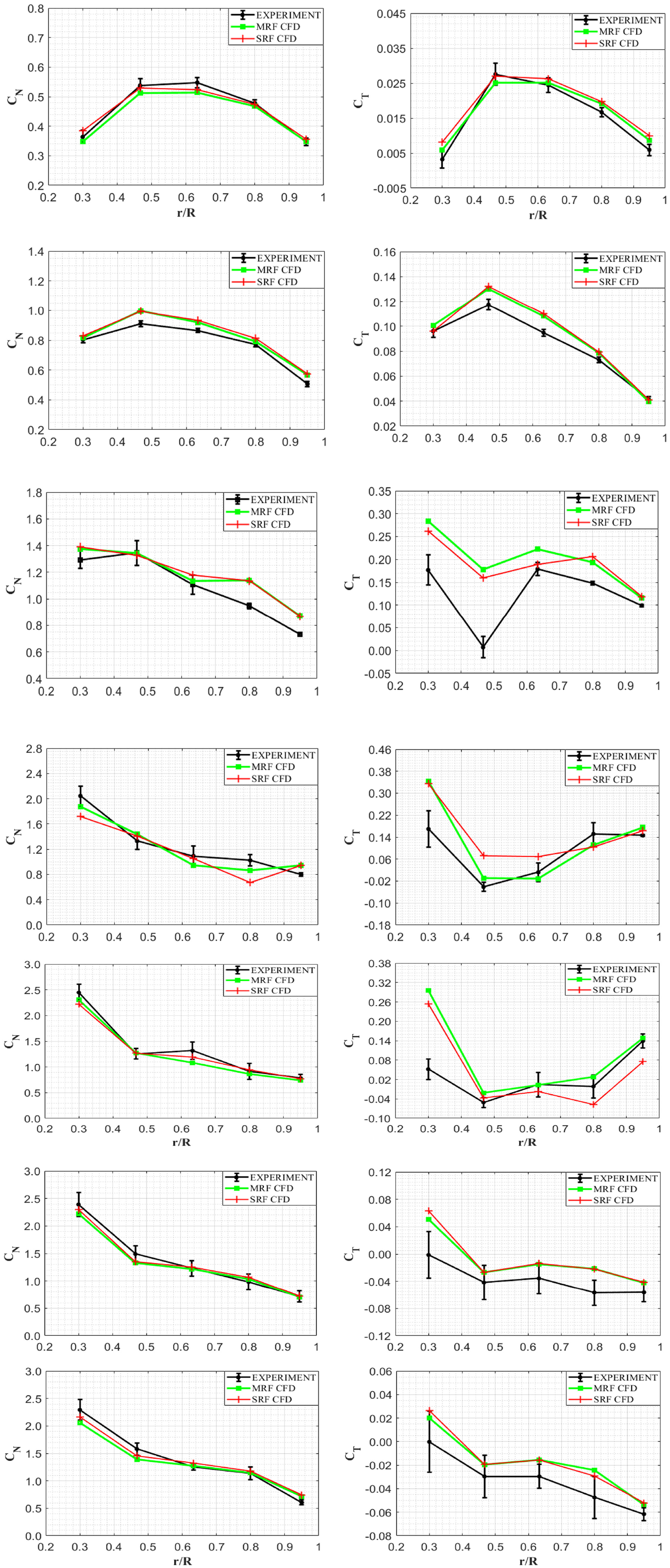
Spanwise distribution of the time-averaged normal (C_N) and tangential (C_T) force coefficients predicted by CFD using the SRF and MRF models compared to the experimental values at seven different wind speeds starting from 5 m/s (top) to 25 m/s (bottom).

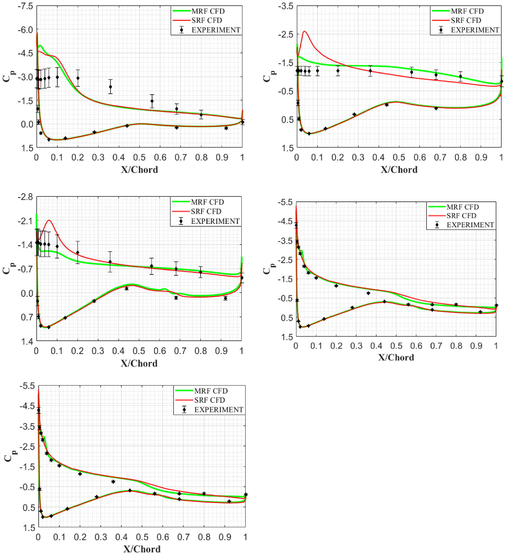
The chordwise static pressure distribution predicted by CFD using SRF and MRF modelling approaches compared to the experimental values at the five different spanwise positions, namely, r/R = 0.3, 0.467, 0.633, 0.8 and 0.95, for the seven wind speed cases are shown in Figures 6 to 12. The measurement uncertainty is again represented using plus/minus one standard deviation. At the lowest wind speeds of 5 m/s and 7 m/s, there is an excellent agreement between SRF and MRF predictions compared to the experimental values, as evident from Figures 5 to 12. The C_N and C_T variations along the blade span are almost correctly captured, qualitatively and quantitatively, using these two modelling approaches. Similarly, the leading edge pressure peaks at the four spanwise locations (i.e. except for the innermost station closest to the root, r/R = 0.3. A possible reason for this is the highly unsteady root vortex flow.) are also accurately predicted using SRF and MRF approaches at these two lowest wind speeds.

Figure 6.

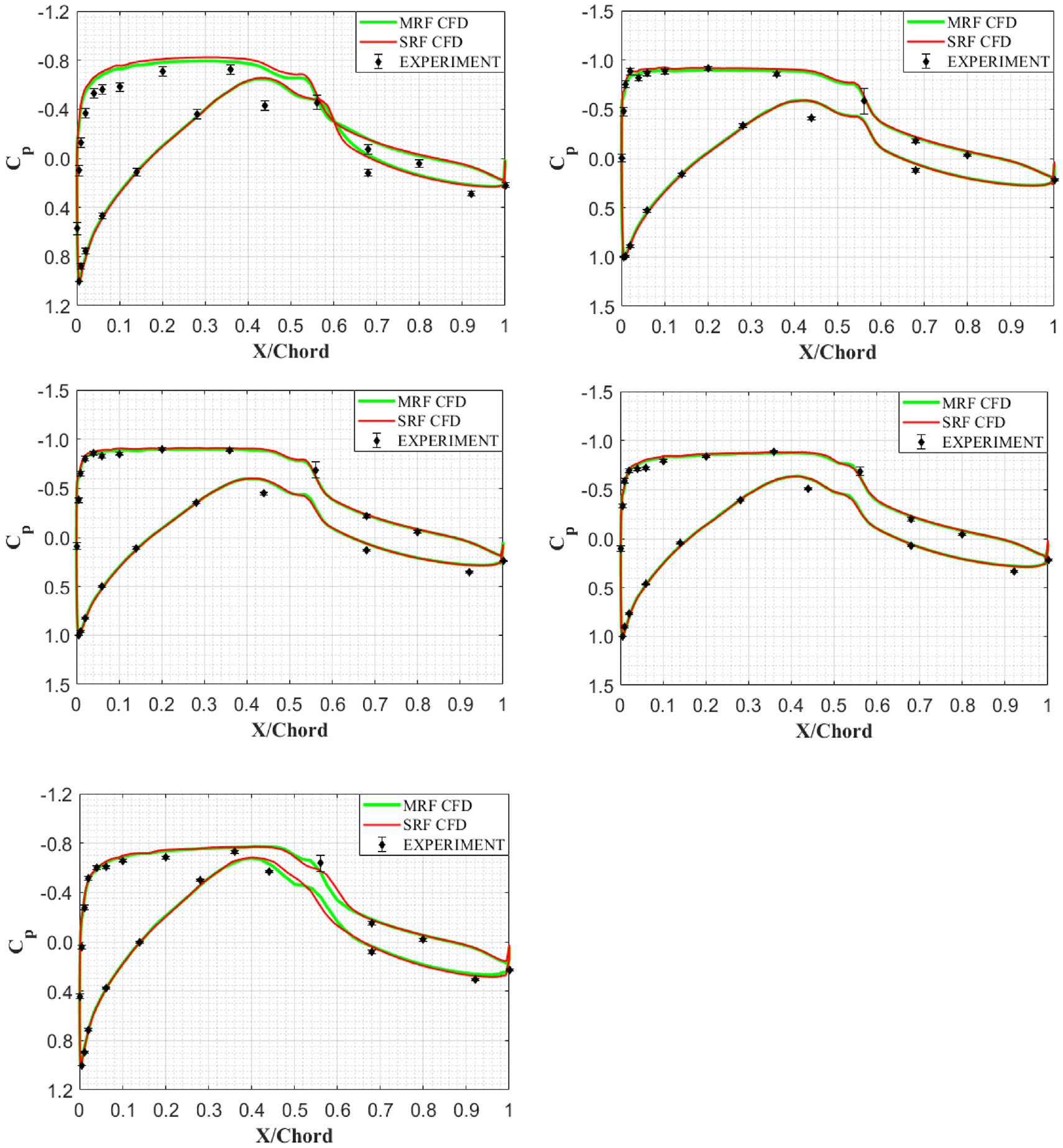
Chord wise distribution of the time-averaged pressure coefficient (C_p) predicted by CFD using the SRF and MRF models compared to the experimental values, both obtained for a wind speed of 5 m/s at spanwise locations of r/R = 0.3 (top left), 0.467 (top right), 0.633 (middle left), 0.8 (middle right) and 0.95 (bottom left). The measurement uncertainty is shown using ±1σ.

Figure 7.

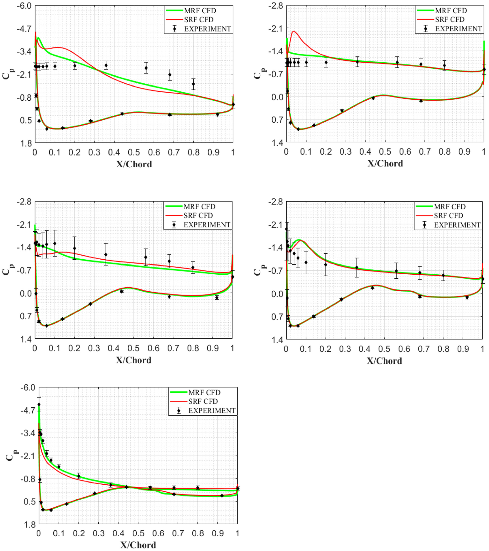
Chord wise distribution of the time-averaged pressure coefficient (C_p) predicted by CFD using the SRF and MRF models compared to the experimental values, both for a wind speed of 7 m/s at spanwise locations of r/R = 0.3 (top left), 0.467 (top right), 0.633 (middle left), 0.8 (middle right) and 0.95 (bottom left). The measurement uncertainty is shown using ±1σ.

Figure 8.

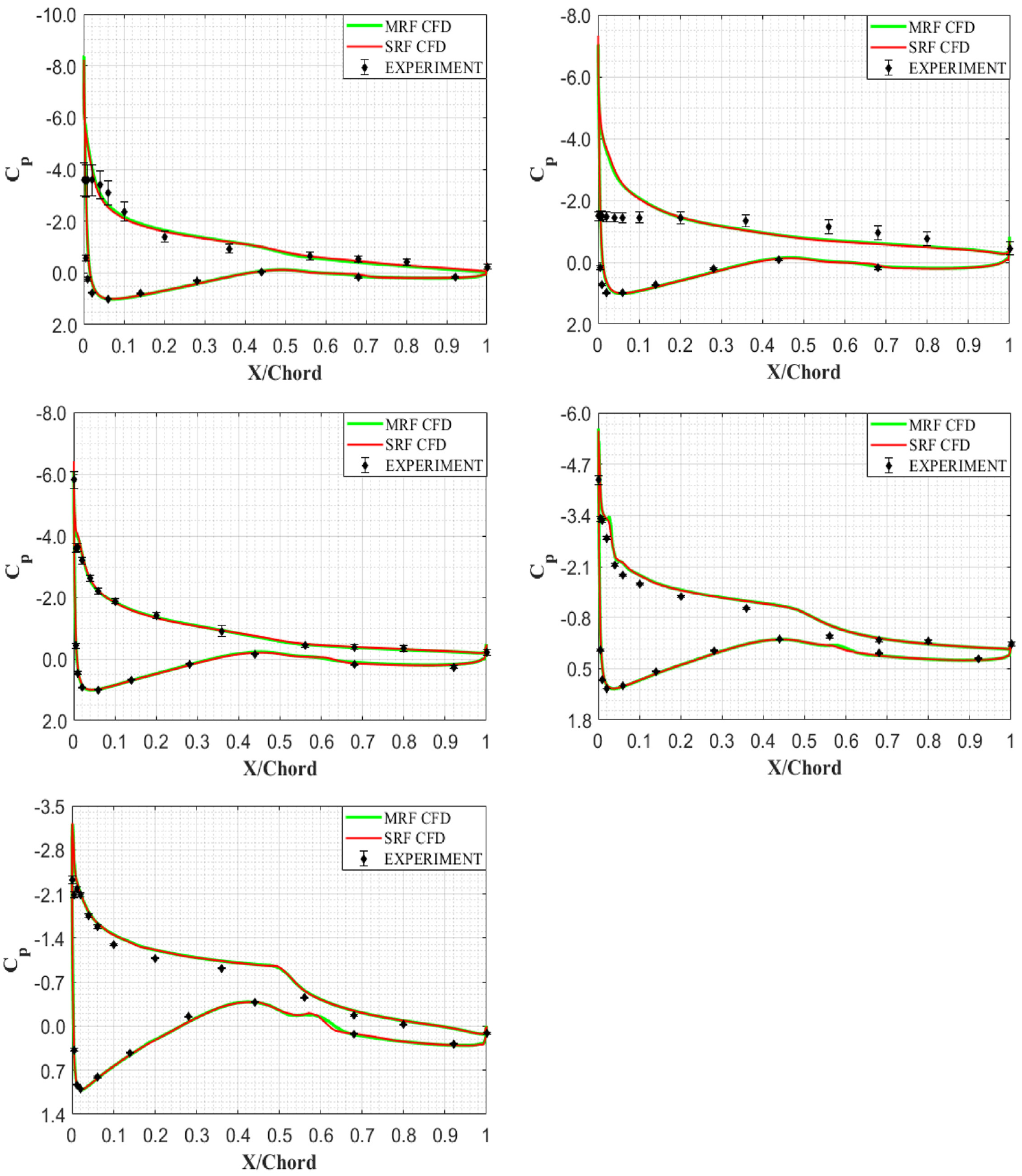
Chord wise distribution of the time-averaged pressure coefficient (C_p) predicted by CFD using the SRF and MRF models compared to the experimental values, both obtained for a wind speed of 10 m/s at spanwise locations of r/R = 0.3 (top left), 0.467 (top right), 0.633 (middle left), 0.8 (middle right) and 0.95 (bottom left). The measurement uncertainty is shown using ±1σ.

Figure 9.

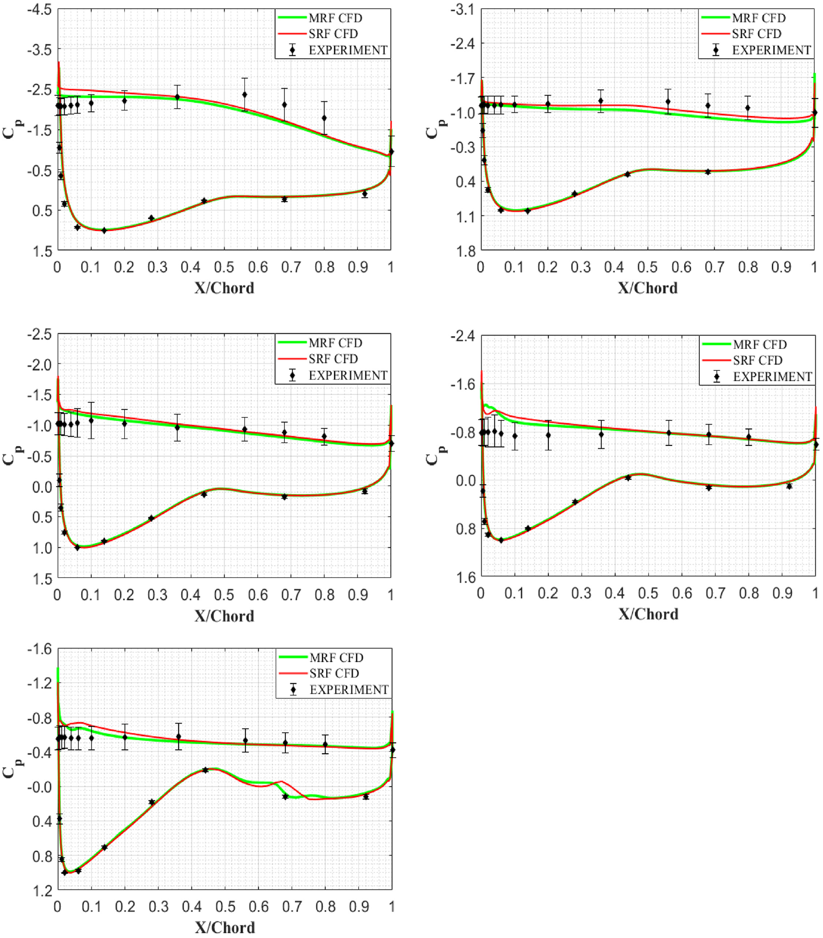
Chord wise distribution of the time-averaged pressure coefficient (C_p) predicted by CFD using the SRF and MRF models compared to the experimental values, both obtained for a wind speed of 13 m/s at spanwise locations of r/R = 0.3 (top left), 0.467 (top right), 0.633 (middle left), 0.8 (middle right) and 0.95 (bottom left). The measurement uncertainty is shown using ±1σ.

Figure 10.

Chord wise distribution of the time-averaged pressure coefficient (C_p) predicted by CFD using the SRF and MRF models compared to the experimental values, both obtained for a wind speed of 15.1 m/s at spanwise locations of r/R = 0.3 (top left), 0.467 (top right), 0.633 (middle left), 0.8 (middle right) and 0.95 (bottom left). The measurement uncertainty is shown using ±1σ.

Figure 11.

Chord wise distribution of the time-averaged pressure coefficient (C_p) predicted by CFD using the SRF and MRF models compared to the experimental values, both obtained for a wind speed of 20.1 m/s at spanwise locations of r/R = 0.3 (top left), 0.467 (top right), 0.633 (middle left), 0.8 (middle right) and 0.95 (bottom left). The measurement uncertainty is shown using ±1σ.

Figure 12.

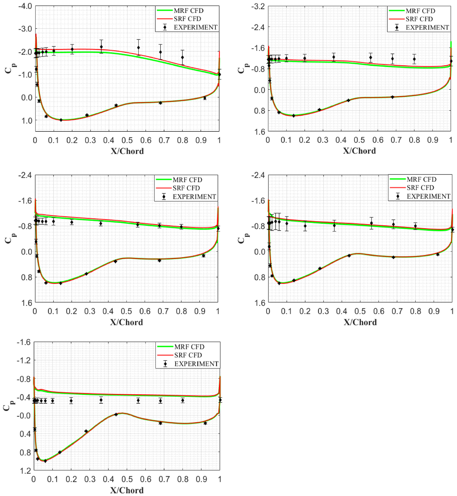
Chord wise distribution of the time-averaged pressure coefficient (C_p) predicted by CFD using the SRF and MRF models compared to the experimental values, both obtained for a wind speed of 25.1 m/s at spanwise locations of r/R = 0.3 (top left), 0.467 (top right), 0.633 (middle left), 0.8 (middle right) and 0.95 (bottom left). The measurement uncertainty is shown using ±1σ.

The reason for such a good agreement between CFD predictions and measurements at low wind speeds is that the flow is mostly attached along the entire blade span except at the innermost station (i.e. at 30% span) located closest to the root. The presence of stalled flow conditions, also called root vortex, on the inboard part of the rotor is evident from the suction side limiting streamlines shown in Figure 14. The small discrepancy observed between CFD predictions and measurements at 30% span can be attributed to the inability of RANS turbulence models to accurately solve separated flows. The turbulence intermittency contour plot on the suction side obtained from SRF and MRF simulations at 7 m/s helps identify the predicted boundary layer transition locations on the blade surface at different spanwise positions. A good agreement between SRF and MRF predictions at low wind speeds is also obvious from these plots.

As the wind speed increases to 10 m/s, a significant discrepancy between CFD predictions and measurements begins to appear around the mid-span region on the suction side of the blade because of the onset of the leading edge stall. The flow separation around the mid-span region is evident from the suction side limiting streamlines obtained using the SRF and MRF modelling approaches, Figure 14. The flow separation thus initiated due to leading-edge stall, and its accompanying localized transient effects, makes it difficult to even detect the suction side pressure peak, as apparent from the r/R = 0.47 station in Figure 8.

Furthermore, the effects of leading-edge stall around the mid-span region are clearly visible in the experimental and CFD predicted values of the tangential force coefficient C_T obtained at 46.7% span, where a sudden dip in C_T serves as a characteristic reminder of its presence around this region. It is apparent that the onset of a stall is not accurately captured in SRF and MRF simulations, even with the inclusion of a Gamma-Theta transition model. The flow over the entire blade is turbulent except for a small portion in the tip region, Figure 13.

Figure 13.

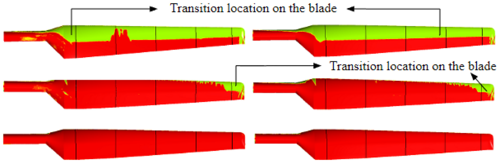
Turbulence intermittency on the suction side predicted by SRF (left) and MRF (right) modelling approaches at wind speeds of 7 m/s (top), 10 m/s (middle) and 20.1 m/s (bottom). The five vertical lines identify the spanwise positions at which surface static pressure is measured.

The boundary layer flow around the mid-span region, in this case, is unstable and very sensitive to even small disturbances (e.g. upstream turbulence levels or blade vibrations or ambient noise) or even to any other minor deviations (e.g. in the manufacturing tolerances of the tested blades, measured mean wind speed levels in the tunnel, etc.). Even a small spanwise shift in the position of the vortices separating near the leading edge would cause changes in the measured static pressure distribution (see limiting streamlines, Figure 14).

Figure 14.

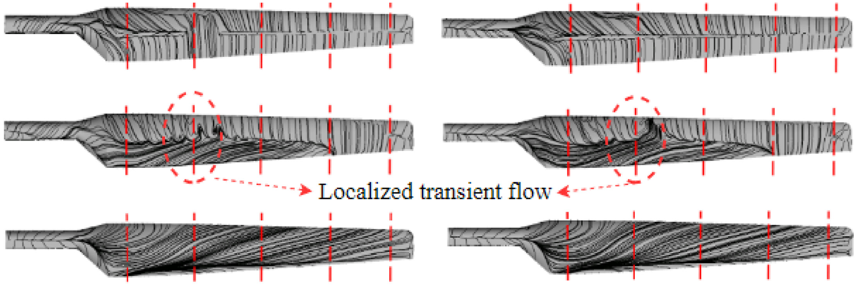
Limiting streamlines on the suction side predicted by SRF (left) and MRF (right) modelling approaches at wind speeds of 7 m/s (top), 10 m/s (middle) and 20.1 m/s (bottom). The five vertical lines identify the spanwise positions at which surface static pressure is measured.

It is worth noting here that a reasonably good agreement between SRF and MRF predictions is seen in all these plots even at 10 m/s. The stall, thus initiated around the mid-span region at 10 m/s, spreads progressively towards the outboard section of the blade surface with an increase in wind speed to 13 m/s, as evidenced by the widening of the characteristic dip in C_T towards the outer span locations.

The wind turbine blade operates in a stall at 13 and 15.1 m/s, with flow separation covering the whole blade surface except around the tip region. Here we start to notice clear differences between SRF and MRF predictions on the suction side towards the inboard sections of the blade. For example, the surface static pressure predicted using the SRF approach contains a peak at 46.7% and 63.3% span that is not present in MRF. A deep stall occurs around the root region at 20.1 and 25.1 m/s, where separated flow persists over the entire blade span including the tip region as evident from the limiting streamlines shown in Figure 14.

As clarified earlier, the deviations in the suction side pressure distribution observed between CFD predictions and measurements in stall and deep stall can be attributed to the problems with RANS turbulence models in accurately solving the separated flows. However, the influence of these deviations on the integrated quantities appears to be minimal as the power predicted by both SRF and MRF still shows surprisingly good agreement with experimental values particularly at the three highest wind speeds of 15.1, 20.1 and 25.1 m/s.

One probable explanation for this could be due to specific stall behaviour characteristics displayed by S809 airfoil at higher angle of attack as noted by Sorenson et al. (2002) and Yelmule and Vsj (2013). A complicated three-dimensional separated flow occurs around the blade tip at higher wind speeds, which is very hard to accurately predict using CFD computations. The deviations seen at the r/R = 0.95 for 20.1 and 25.1 m/s can be attributed to the inability of SRF and MRF models to resolve the tip flow field correctly.

As seen in Figure 5, quantitative differences exist between the experimental data and the CFD-predicted results of normal and tangential force coefficients. However, the overall qualitative trend is still correctly captured using both SRF and MRF approaches at all seven wind speeds. The force coefficients at any spanwise position obtained from experiments are calculated only from 22 surface static pressure measurements, assuming a linear variation between any two adjacent pressure taps. At the same time, CFD computations were performed with ∼600 grid points along the airfoil. Finally, it is worth noting that the sectional force coefficients predicted by SRF and MRF models at all wind speeds are very similar to the values reported by Sorenson et al. (2002) and Yelmule and Vsj (2013).

2D airfoil characteristics extracted from CFD

The S809 airfoil polars extracted from 3D CFD computations using SRF and MRF models at five different spanwise positions of r/R = 0.29, 0.48, 0.66, 0.79 and 0.93 are shown in Figure 15. These 2D aerodynamic characteristics are obtained using the methodology described by Johansen and Sørensen (2004). Also included in Figure 15 are the polar curves for the S809 airfoil with natural transition obtained at a Re = 1E6 in the OSU wind tunnel.

Figure 15.

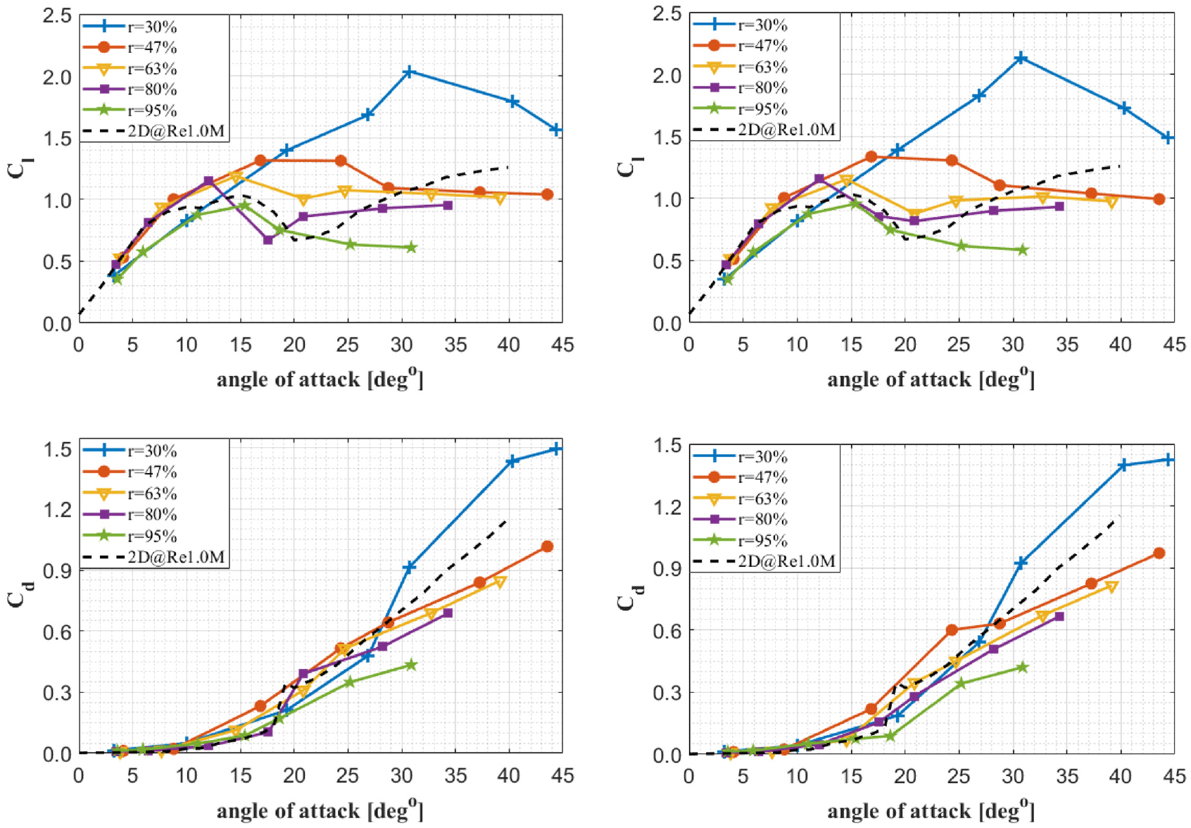
Local polars at five different radial positions extracted from three-dimensional CFD computations using SRF (left) and MRF (right) models.

At the innermost radial location, the lift and drag coefficients predicted by CFD using SRF and MRF approaches at larger angles of attack are greater than the corresponding wind tunnel measurement values. According to Johansen and Sørensen (2004), a probable explanation for this is the stall delay occurring on the inboard section caused by 3D rotational effects, also called ‘Himmelskamp effect’ (Himmelskamp, 1947). The two spanwise locations least affected by the radial flow expected to occur near the root and tip regions are r/R = 0.63 and 0.79. Our CFD predictions show good agreement with the wind tunnel data at these two radial stations. Moving outboard towards the tip, the induced 3D effects from the tip vortices are expected to cause a decrease in the computed lift coefficients. The maximum C_l and the corresponding angle of attack predicted by CFD show a drop approaching values comparable to the 2D airfoil data. Again, the C_l values computed from CFD near the blade tip at r/R = 0.95 are slightly smaller than the corresponding 2D airfoil characteristics due to the 3D-induced effects of tip vortices. Also, a rapid increase in C_d with the angle of attack is evident in Figure 15.

Conclusion

A series of results from the CFD analysis of NREL Phase-VI rotor in upwind configuration with 0° yaw misalignment and a blade tip pitch angle of 3° is documented. These computations are accomplished using a 3D unstructured uRANS solver coupled with SST κ-ω turbulence model and a Gamma-Theta transition model. The simulations were performed in the ANSYS CFX 2021 R1 to validate against the NREL Test Sequence-S measurements using two moving reference frame modelling approaches, SRF and MRF. The results computed using both these approaches (SRF slightly better than MRF) show a good qualitative and quantitative agreement with the measurements at six of the seven tested wind speeds. The only exception is the 10 m/s wind speed case. At low wind speeds (i.e. 5 and 7 m/s), the flow over the rotor blade is mostly attached except on the inboard part of the rotor, as confirmed by the limiting streamlines. The time-averaged CFD predictions obtained from SRF and MRF models show an excellent agreement with the corresponding experimental values at these two wind speeds. As the wind speed increases to 10 m/s, a massive flow separation appears on the suction side near the leading edge close to the mid-span region. This is seen in both SRF and MRF approaches, as evidenced by the limiting streamlines obtained at 10 m/s. The boundary layer flow around the mid-span region is unstable and very sensitive to even small disturbances (e.g. upstream turbulence levels or blade vibrations or ambient noise) or even to any other very small variations (e.g. in the manufacturing tolerances of the tested blades, measured mean wind speed levels in the tunnel, etc.). Thus, the discrepancy between CFD predictions and measurements at 10 m/s is attributed to the inability of uRANS turbulence models to solve separated flows accurately and also due to the presence of transient effects accompanying the flow separation. The inclusion of the Gamma-Theta transition model is insufficient to close the gap between CFD predictions and measurements at 10 m/s. The separation, thus initiated at 10 m/s around the mid-span region, progressively grows with an increase in the upstream wind speed to engulf the entire blade. The blade is in a deep stall at 20.1 and 25.1 m/s, as evinced by the limiting streamlines obtained at these two wind speeds. The quantitative differences observed in the static pressure distribution on the suction side are attributed to the specific stall behaviour of the S809 airfoil. These CFD simulations provide deeper insight into the complex 3D effects of the wind flow interaction with a rotating, twisted, and tapered rotor. The validated SRF and MRF models of the two-bladed wind turbine developed here will be employed to understand and evaluate the effects of minor design changes (e.g. a modified tip design or inclusion of vortex generators) on a wind turbine’s performance, to evaluate the performance of diffuser-augmented wind turbines and also in wind farm-level studies.

Footnotes

Appendix

Table A1.

Operating input conditions for SRF and MRF simulations.

Runs	Wind speed (m/s)	Angular speed (rpm)	Density (kg/m³)
S05	5	71.7	1.243
S07	7	71.9	1.246
S10	10	72.1	1.246
S13	13	72.1	1.227
S15	15.1	72.1	1.224
S20	20.1	72	1.221
S25	25.1	72.1	1.220

Declaration of conflicting interests

The author(s) declared no potential conflicts of interest with respect to the research, authorship, and/or publication of this article.

Funding

The author(s) disclosed receipt of the following financial support for the research, authorship, and/or publication of this article: The authors thank the Science and Engineering Research Board (SERB), Department of Science and Technology, New Delhi [Grant No.ECR/2018/000819] for the financial Support.

ORCID iD

Mujahid Shaik

References

GWEC, (2017) Global Wind Report 2019. Brussels: GWEC, p. 637.

ANSYS Inc (2021a) ANSYS CFX-Solver manager User’s Guide, Release 20.1.

ANSYS Inc (2021b) ANSYS CFX-Solver Theory Guide, Release 2021 R1.

ANSYS Inc (2021c) ANSYS Fluent Theory Guide, Release 2021 R1.

ANSYS Inc (2021d) ICEM CFD Help Manual, Release 2021 R1.

ANSYS Inc (2021e) ICEM CFD User’s Manual, Release 2021 R1.

Bechmann

Sørensen

Zahle

(2011) Cfd simulations of the MEXICO rotor. Wind Energy 14(5): 677–689.

Duque

EPN

Burklund

Johnson

(2003) Navier-Stokes and comprehensive analysis performance predictions of the NREL phase VI experiment. Journal of Solar Energy Engineering 125(4): 457–467.

Eleni

Athanasios

Dionissios

(2012) Evaluation of the turbulence models for the simulation of the flow over a National Advisory Committee for Aeronautics (NACA) 0012 airfoil. Journal of Mechanical Engineering Research 4(3): 100–111.

10.

Gerber

Tangler

Duque

EPN

, et al. (2005) Peak and post-peak power aerodynamics from phase VI NASA Ames wind turbine data. Journal of Solar Energy Engineering 127(2): 192–199.

11.

Gielen

Gorini

Wagner

, et al. (2018) Global Energy Transformation: A Roadmap to 2050. Abu Dhabi: International Renewable Energy Agency.

12.

Hand

Simms

Fingersh

, et al. (2001) Unsteady aerodynamics experiment phase VI: Wind tunnel test configurations and available data campaigns. In: National Renewable Energy Lab., No. NREL/TP-500-2995. Golden, CO, USA.

13.

Himmelskamp

(1947) Profile Investigations on a Rotating Airscrew. Ministry of Aircraft Production.

14.

Johansen

Sørensen

(2004) Aerofoil characteristics from 3D CFD rotor computations. Wind Energy 7(4): 283–294.

15.

Lanzafame

Mauro

Messina

(2013) Wind turbine CFD modeling using a correlation-based transitional model. Renewable Energy 52: 31–39.

16.

Menter

(1993) Zonal two equation kw turbulence models for aerodynamic flows. In: 23rd fluid dynamics, plasmadynamics, and lasers conference, p.2906.

17.

Menter

(1994) Two-equation eddy-viscosity turbulence models for engineering applications. AIAA Journal 32(8): 1598–1605.

18.

Lee

(2012) Cfd investigation on the aerodynamic characteristics of a small-sized wind turbine of NREL PHASE VI operating with a stall-regulated method. Journal of Mechanical Science and Technology 26(1): 81–92.

19.

Ohya

Karasudani

(2010) A shrouded wind turbine generating high output power with wind-lens technology. Energies 3(4): 634–649.

20.

Ohya

Karasudani

Nagai

, et al. (2017) Wind lens technology and its application to wind and water turbine and beyond. Renewable Energy and Environmental Sustainability 2(2): 2.

21.

Potsdam

Mavriplis

(2009) Unstructured mesh CFD aerodynamic analysis of the NREL Phase VI rotor. In: 47th AIAA Aerospace Sciences Meeting Including The New Horizons Forum and Aerospace Exposition, p.1221.

22.

Sadorsky

(2021) Wind energy for sustainable development: Driving factors and future outlook. Journal of Cleaner Production 289: 125779.

23.

Schepers

Boorsma

Gomez-Iradi

, et al. (2014) Final report of IEA Task 29, Mexnext (Phase 2). ECN-E-14-060, Energy Research Center of the Netherlands.

24.

Simms

Schreck

Hand

, et al. (2001) NREL unsteady aerodynamics experiment in the NASA-Ames wind tunnel: A comparison of predictions to measurements. In: National Renewable Energy Lab., No. NREL/TP-500-29494, Golden, CO, United States.

25.

Song

Perot

(2015) Cfd simulation of the NREL phase VI rotor. Wind Engineering 39(3): 299–309.

26.

Subramanian

Chokani

Abhari

(2015) Drone-based experimental investigation of three-dimensional flow structure of a multi-megawatt wind turbine in complex terrain. Journal of Solar Energy Engineering 137(5): 1–10.

27.

Sørensen

(2008) CFD modeling of laminar-turbulent transition for airfoils and rotors using the γ-θ Model. In: 26th AIAA applied aerodynamics conference, p.7323.

28.

Sørensen

Michelsen

Schreck

(2002) Navier-Stokes predictions of the NREL phase VI rotor in the NASA Ames 80 ft × 120 ft wind tunnel. Wind Energy 5(2-3): 151–169.

29.

Taylor

(1997) Introduction to error analysis, the study of uncertainties in physical measurements.

30.

DAVID

Wilcox

(1991) A half century historical review of the k-omega model. In: 29th Aerospace Sciences Meeting, p.615.

31.

Sankar

(2000) Computational study of horizontal axis wind turbines. Journal of Solar Energy Engineering 122(1): 35–39.

32.

Yelmule

Vsj

(2013) CFD predictions of NREL phase VI rotor experiments in NASA/AMES wind tunnel. International Journal of Renewable Energy Research 3(2): 261–269.

33.

Zhang

Sun

van Zuijlen

, et al. (2017) Numerical simulation of transitional flow on a wind turbine airfoil with RANS-based transition model. Journal of Turbulence 18(9): 879–898.

34.

Zhong

Tang

Wang

, et al. (2018) Accurate RANS simulation of wind turbine stall by turbulence coefficient calibration. Applied Sciences 8(9): 1444.

35.

Zhou

(2017) Investigation of applying CFD models to 3D wind turbine simulation. Doctoral dissertation, UNSW Sydney.

36.

Zhu

Chen

Qiu

, et al. (2021) Numerical investigation into rotational augmentation with passive vortex generators on the NREL Phase VI blade. Energy 223: 120089.