Forecast of wind speed based on MLP network model using Levenberg Marquardt and gradient descent algorithms in Tetouan city,Northern Morocco

Abstract

This study aims to find the most powerful algorithm between LM and GD, applying them to the multilayer neural network (MLP) to predict the wind speed of the city of Tetouan. To achieve this we will use the meteorological data of this city from 31/07/2017 to 31/08/2022. The MLP adopted for our study is composed of two hidden layers, 30 neurons in the first layer and 15 in the second, 7 inputs and one output. The data is divided into 80% for training and 20% for testing. The results obtained showed that the Levenberg-Marquardt (LM) algorithm is more efficient than the gradient descent (GD) algorithm with a correlation coefficient R = 0.988102 and a mean square error MSE = 0. 0458. These results will allow us to accurately predict the wind speed of August for the year 2022 in this city.

Keywords

Artificial neural network feedforward neural network multi-layer perceptron (MLP)wind speed prediction optimization algorithm

Introduction

Nowadays, the importance of producing energy from renewable sources is immense for all countries. The promotion of sustainability and environmental health is not the only benefit, but it also promotes economic resilience, energy autonomy, and a more sustainable future for all.

Our research will focus on wind energy, and we chose Tetouan City as the location due to its geographical favorableness for wind energy. The meteorological environment at the chosen site is particularly diverse, so to optimize the use of wind energy in this particular region, it is crucial to have accurate wind speed prediction.

Various methods are established to improve the accuracy of wind speed prediction, including time series techniques such as persistence, ARMA (Autoregressive Moving Average), gray predictor, and Kalman filter. Additionally, machine learning methods such as RNA (Recurrent Neural Networks), RNA-fuzzy, SVM (Support Vector Machines), and others include spatial correlation. (Beauregard-Harvey, 2018).

The effectiveness of these methods depends on the time horizon studied. In this context, we carried out a short-term study based on Tetouan’s historical data, our choice for wind speed forecasting was neural networks because of their ability to control variables with stochastic characteristics.

To predict the future values of wind speed, the MLP model, which is a feed-forward neural network, is used.

We implemented it each time using the two famous algorithms LM and GD in MATLAB on the meteorological data of Tetouan city for 5 years.

In this context, we conducted a short-term study using neural networks, which have proven to be highly relevant and powerful. The study is based on historical data to predict wind speed which has stochastic characteristics. Specifically, we employed a multilayer perceptron (MLP) implemented each time by the two famous algorithms LM (Levenberg-Marquardt) and GD (Gradient Descent). The training was performed in MATLAB using meteorological data from the city of Tetouan over 5 years.

The purpose of this article is to find answers to the following questions:

Is the MLP application suitable to process the data of this site? If yes, which is the most powerful algorithm among LM and GD, and which gives a good accuracy? (Salami et al., 2017).

Methodology

Theoretical study

The multilayer perceptron

A non-looped or forward propagating artificial neural network is constructed of three essential layers, the input layer in the form of variable values (are not neurons) which does not perform any calculation, a hidden layer (or more than one layer), and an output layer. The neurons of each layer are interconnected, while the nodes of the same layer are independent (Qu’est-ce qu’un réseau neuronal artificiel ? - IONOS, n.d.)

The general mathematical model of the multilayer perceptron is illustrated in the diagram below (Figure 1).

Figure 1.

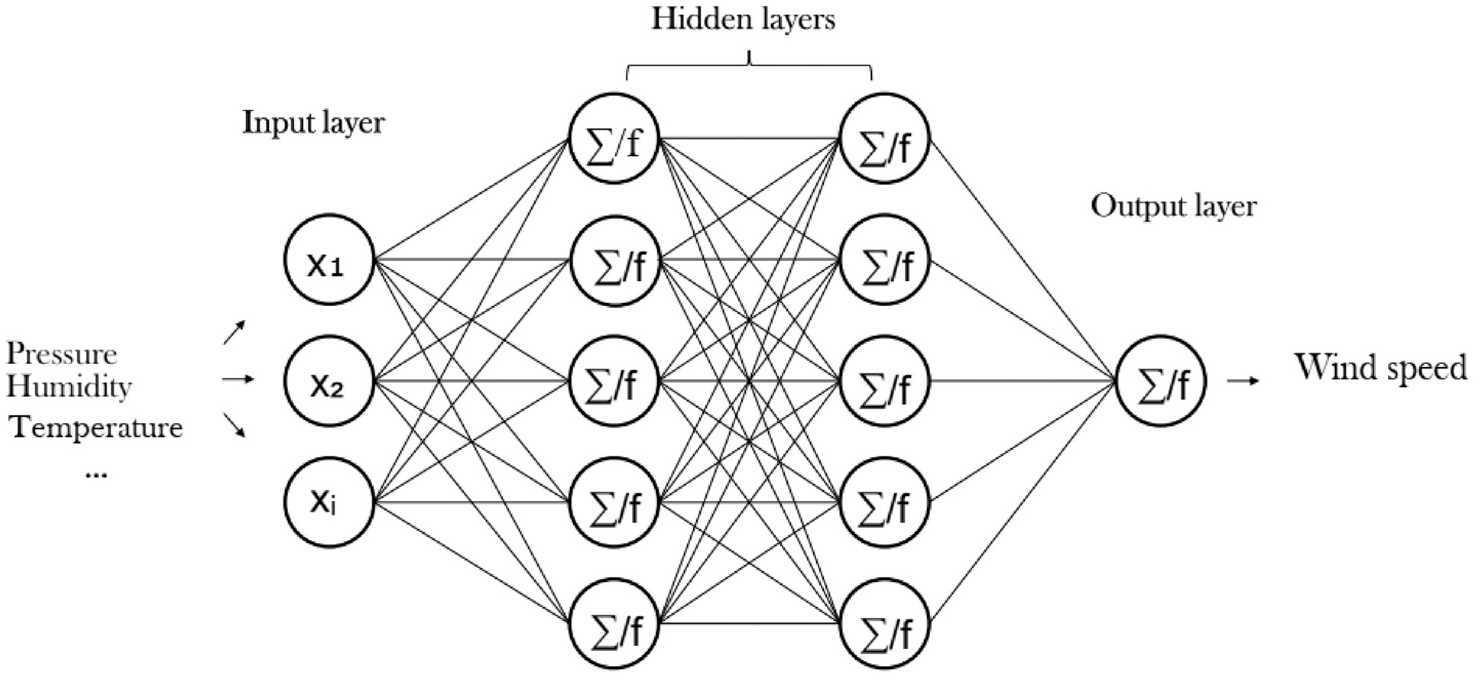
The structure of a multilayer artificial neural network (Beauregard-Harvey, 2018).

The desired output can be calculated by applying the following equation:

y = f (S) = f (\sum w_{ij} x_{i} + b_{i})

(1)

There:

S: Summation function

X_i: Inputs of the neural network

y: The output of the network

w_ij: The connection weights associated with each input.

b_i: Bias (threshold)

f: The hyperbolic-tangent transfer function that allows the neural network to solve complicated models, using the equation:

f = \frac{e^{x} + e^{- x}}{e^{x} + e^{- x}}

(2)

The mathematical model chosen for our study is illustrated in the diagram below (Figure 2).

Figure 2.

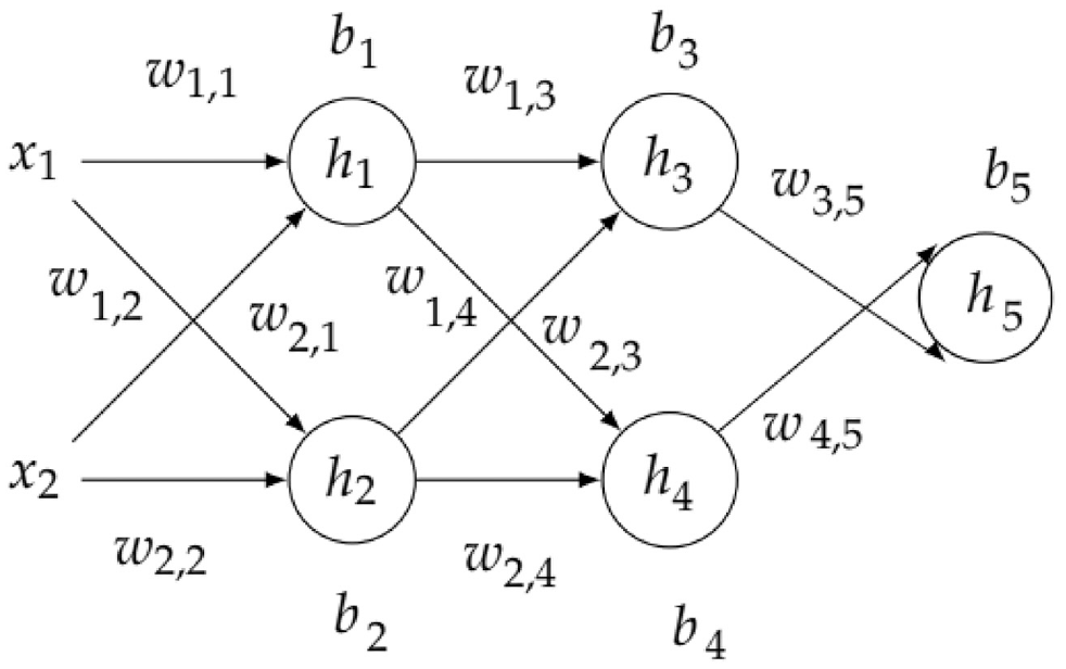
The perceptron with two hidden layers. (Nasr, n.d.).

To obtain the output of each layer, we apply the following mathematical relationships:

h 1 = f (w 1, 1 . x 1 + w 2, 1 . x 2 + b 1)

(3)

h 2 = f (w 1, 2 . x 1 + w 2, 2 . x 2 + b 2)

(4)

h 3 = f (w 1, 3 . h 1 + w 2, 3 . h 2 + b 3)

(5)

h 4 = f (w 1, 4 . h 1 + w 2, 4 . h 2 + b 4)

(6)

h 5 = f (w 3, 5 . h 3 + w 4, 5 . h 4 + b 5)

(7)

During the learning phase, the output of a neuron must exceed the specified threshold to activate, thus allowing the next layer to receive information that propagates in the same direction, so each output represents the input of the neuron that follows it, which justifies the process of forward propagation or feedforward of this model (Nasr, n.d.).

In this article, we try to improve the performance of the neural network by reducing the total error which can be calculated by:

MSE (mean square error) = \frac{1}{n} \sum_{1}^{n} {(Y - Ypred)}^{2}

(8)

RMSE (root mean square error) = \sqrt{\frac{1}{n}} \sum_{1}^{n} {(Y - Ypred)}^{2}

(9)

MAE (Absolu squared error) = \frac{1}{n} \sum_{1}^{n} | (Y - Ypred) |

(10)

Practical study using Matlab

Data preprocessing and normalization

The prediction gives a primordial importance to the preprocessing of the data, it is the first step to be carried out in this study. The collected data are pre-processed via EXCEL to eliminate some non-numerical variables disturbing the learning of the chosen model, and which are in a certain format not acceptable by MATLAB.

After the pre-processing phase, the data with variable scales will be transformed into other appropriate data of comparable scales before providing them to the learning algorithm, so that we can analyze them simply (Ren et al., 2009; Salami et al., 2017).

We will normalize them in an interval [−1,1] via the following relation.

Xnorm = \frac{X_{i} - μ_{i}}{s_{i}} (Alboukadel, 2020)

(11)

With :

X_i: Original data

μ_{i} = \frac{\sum X_{i}}{n b r (X_{i})}

(12)

S_{i} = X m a x - X m i n

(13)

Choice of variables for the prediction model

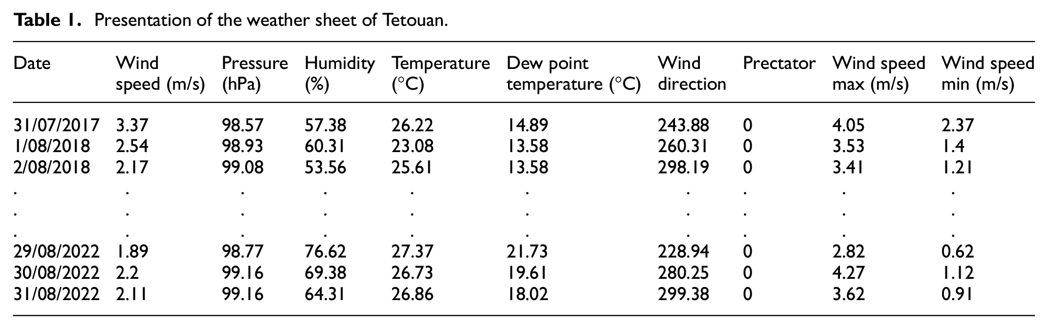
We processed the weather data of the city of Tetouan from 31/07/2017 to 31/08/2022 obtained from the site https://power.larc.nasa.gov/data-access-viewer/ (Table 1).

Table 1.

Presentation of the weather sheet of Tetouan.

Date	Wind speed (m/s)	Pressure (hPa)	Humidity (%)	Temperature (°C)	Dew point temperature (°C)	Wind direction	Prectator	Wind speed max (m/s)	Wind speed min (m/s)
31/07/2017	3.37	98.57	57.38	26.22	14.89	243.88	0	4.05	2.37
1/08/2018	2.54	98.93	60.31	23.08	13.58	260.31	0	3.53	1.4
2/08/2018	2.17	99.08	53.56	25.61	13.58	298.19	0	3.41	1.21
.	.	.	.	.	.	.	.	.	.
.	.	.	.	.	.	.	.	.	.
.	.	.	.	.	.	.	.	.	.
29/08/2022	1.89	98.77	76.62	27.37	21.73	228.94	0	2.82	0.62
30/08/2022	2.2	99.16	69.38	26.73	19.61	280.25	0	4.27	1.12
31/08/2022	2.11	99.16	64.31	26.86	18.02	299.38	0	3.62	0.91

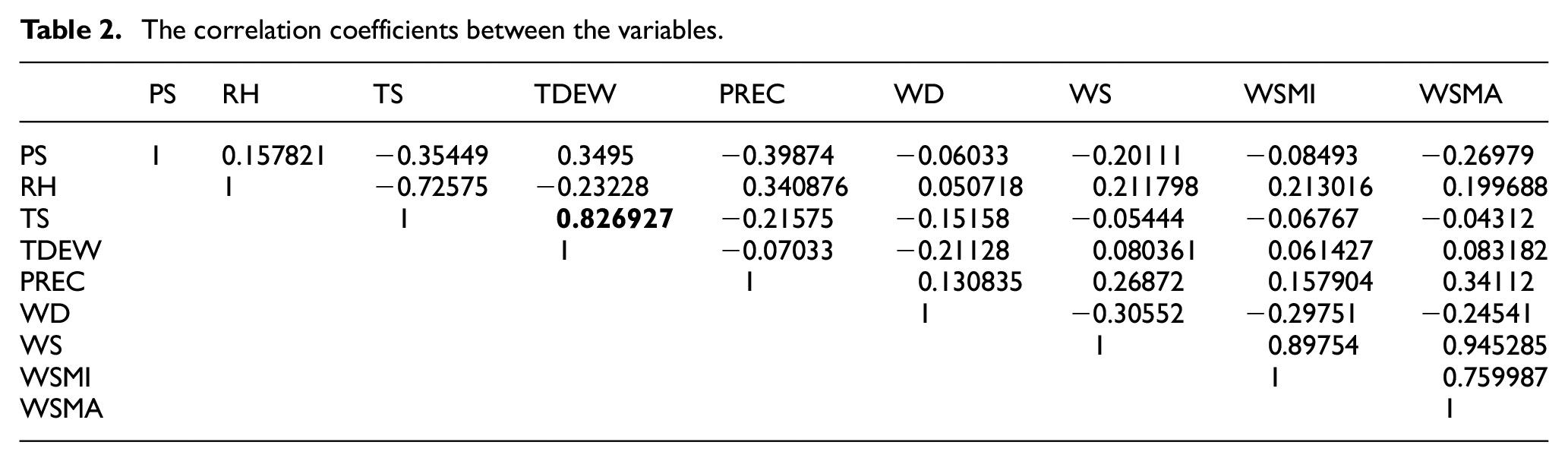
From the table of variables below (Table 2), we notice that the dew temperature and the wind temperature have a coefficient R = 0.826927, this value shows that these two variables have the same climatological characteristics, so they have the same effect on the desired output which allows us to eliminate one of them to avoid all the expensive calculations (Amellas et al., 2020a).

Table 2.

The correlation coefficients between the variables.

	PS	RH	TS	TDEW	PREC	WD	WS	WSMI	WSMA
PS	1	0.157821	−0.35449	0.3495	−0.39874	−0.06033	−0.20111	−0.08493	−0.26979
RH		1	−0.72575	−0.23228	0.340876	0.050718	0.211798	0.213016	0.199688
TS			1	0.826927	−0.21575	−0.15158	−0.05444	−0.06767	−0.04312
TDEW				1	−0.07033	−0.21128	0.080361	0.061427	0.083182
PREC					1	0.130835	0.26872	0.157904	0.34112
WD						1	−0.30552	−0.29751	−0.24541
WS							1	0.89754	0.945285
WSMI								1	0.759987
WSMA									1

The inputs of the model include seven variables, pressure, relative humidity, surface temperature, precipitation, wind direction, maximum and minimum wind speed all at time t. The output is the wind speed that we want to predict at the same time t (Salami et al., 2017).

Programing steps Result and discussion

After preparing the program as shown in (Figure 3), we performed several tests by increasing the number of input variables from five inputs; pressure, temperature, humidity, precipitation, and wind direction; to seven inputs; pressure, temperature, humidity, precipitation, wind direction, minimum wind speed, and maximum wind speed. Thus we changed every time, the number of hidden layers and neurons for each hidden layer, we found that the model has a good performance with seven inputs, two hidden layers with 30 neurons at the first layer and 15 at the second for both algorithms (Figure 4) (Amellas et al., 2020b).

Figure 3.

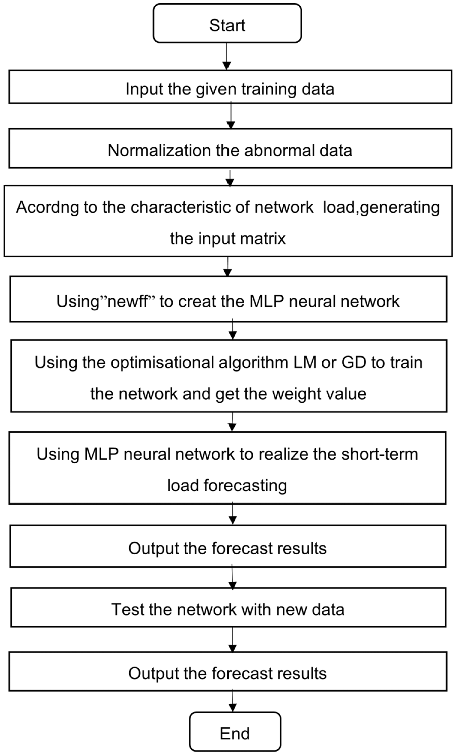
The flowchart of the short-term output prediction program is valid for both algorithms (Ren et al., 2009).

Figure 4.

MLP -2 hidden layers- (30,15) neurons-Tansig activation function.

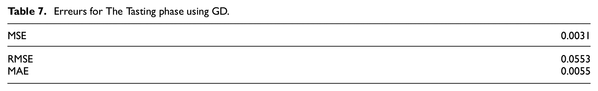
MSE, RMSE, and MAE are errors that show the difference between the actual output and the desired output, we have calculated them for the training and testing phases as shown in Tables 3, 5 and 7.

Table 3.

The training results were obtained by the two algorithms LM and GD

Day	Y (m/s)	Y_{d LM} (m/s)	Y_{d GD} (m/s)	E_LM	E_GD
31/08/2017	4.2800	4.0896	4.5494	0.0458	0.1101	MSE
1/09/2017	4.9300	5.1166	5.2459	0.2139	0.3318	RMSE
2/09/2017	5.9100	5.9859	5.7312	0.1545	0.2466	MAE

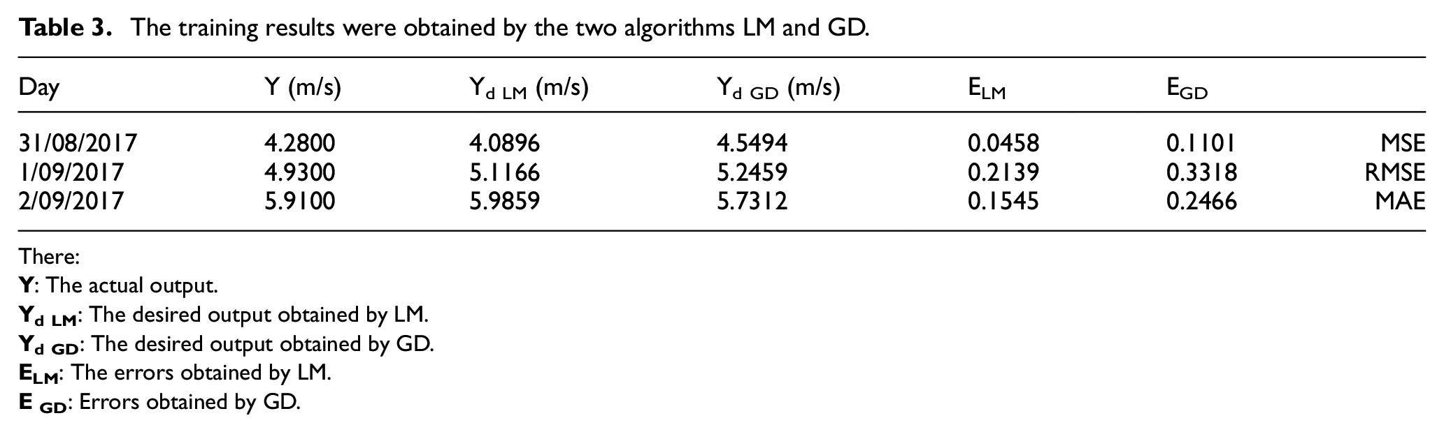
There:

Y: The actual output.

Y_{d LM} : The desired output obtained by LM.

Y_{d GD} : The desired output obtained by GD.

E_LM: The errors obtained by LM.

E_GD: Errors obtained by GD.

The values of coefficient R obtained for the three phases; training, validation, and test are 0.99102, 0.98269, and 0.97673 for LM, 0.97213, 0.97316, and 0.97526 for GD (Figures 5 and 8) these values are close to 1, which shows the strong relationship between the actual and desired output (Figures 6 and 9); consequently, the model chosen for Tetouan city is capable of predicting the wind speed (Amellas et al., 2020b).

Figure 5.

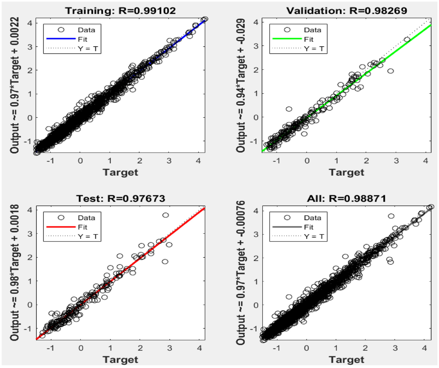
The diagram of the regression obtained by the LM algorithm.

Figure 6.

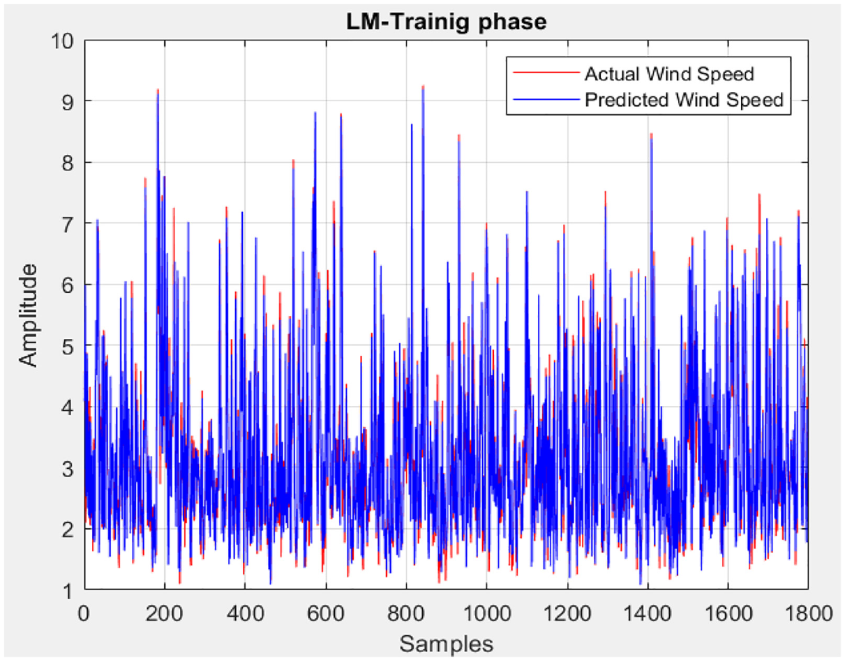
Wind speed prediction obtained by the LM algorithm.

Figure 7 shows that the error decreases after more training epochs but in the case of LM, we notice that it can start to increase on the validation data set when the network starts to overfit the training data. In this case, the training stops after 31 consecutive increases in the validation error, and the best performance of value 0.036094 is obtained from the 11 epoch where the value of the validation error is the lowest (Analyze Shallow Neural Network Performance After Training - MATLAB & Simulink - MathWorks Benelux, n.d.). For the case of GD, the program needs to do 1000 epochs to reach the good performance of value 0.054519 as shown in Figure 10.

Figure 7.

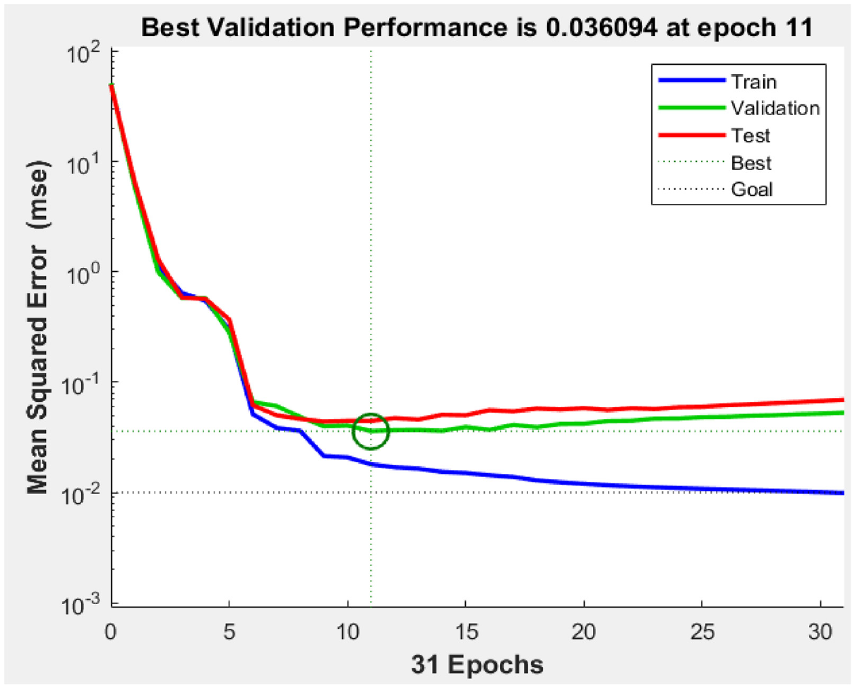
The performance graph obtained by the LM algorithm.

Figure 8.

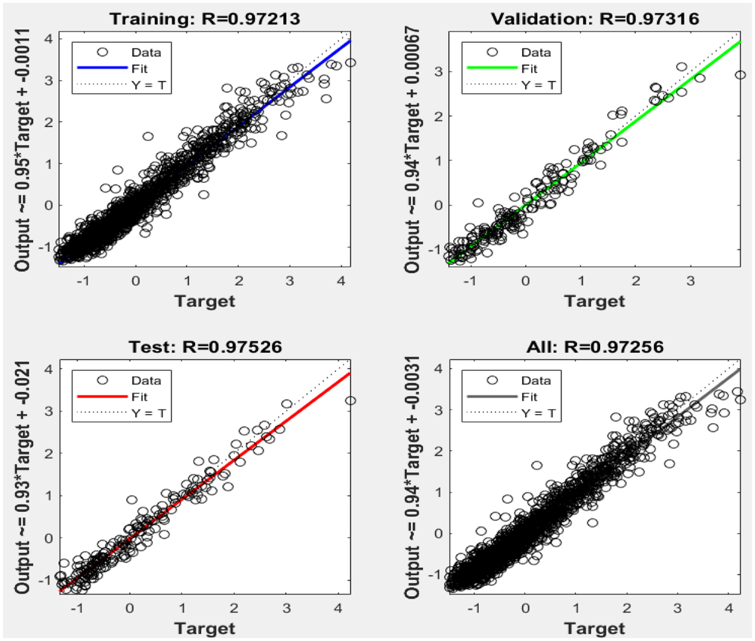
The regression diagram obtained by the GD algorithm.

Figure 9.

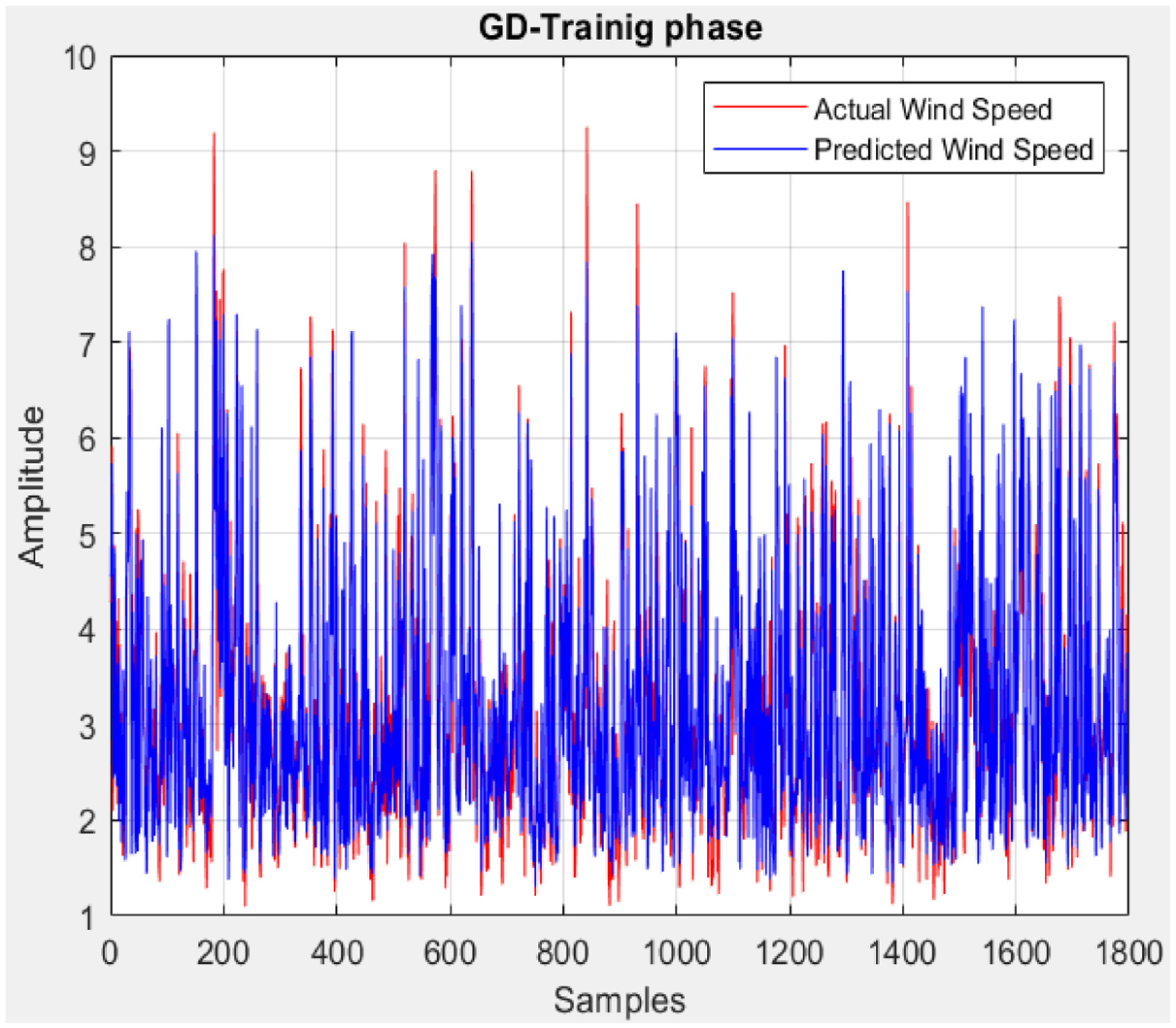
Wind speed prediction obtained by the GD algorithm.

Figure 10.

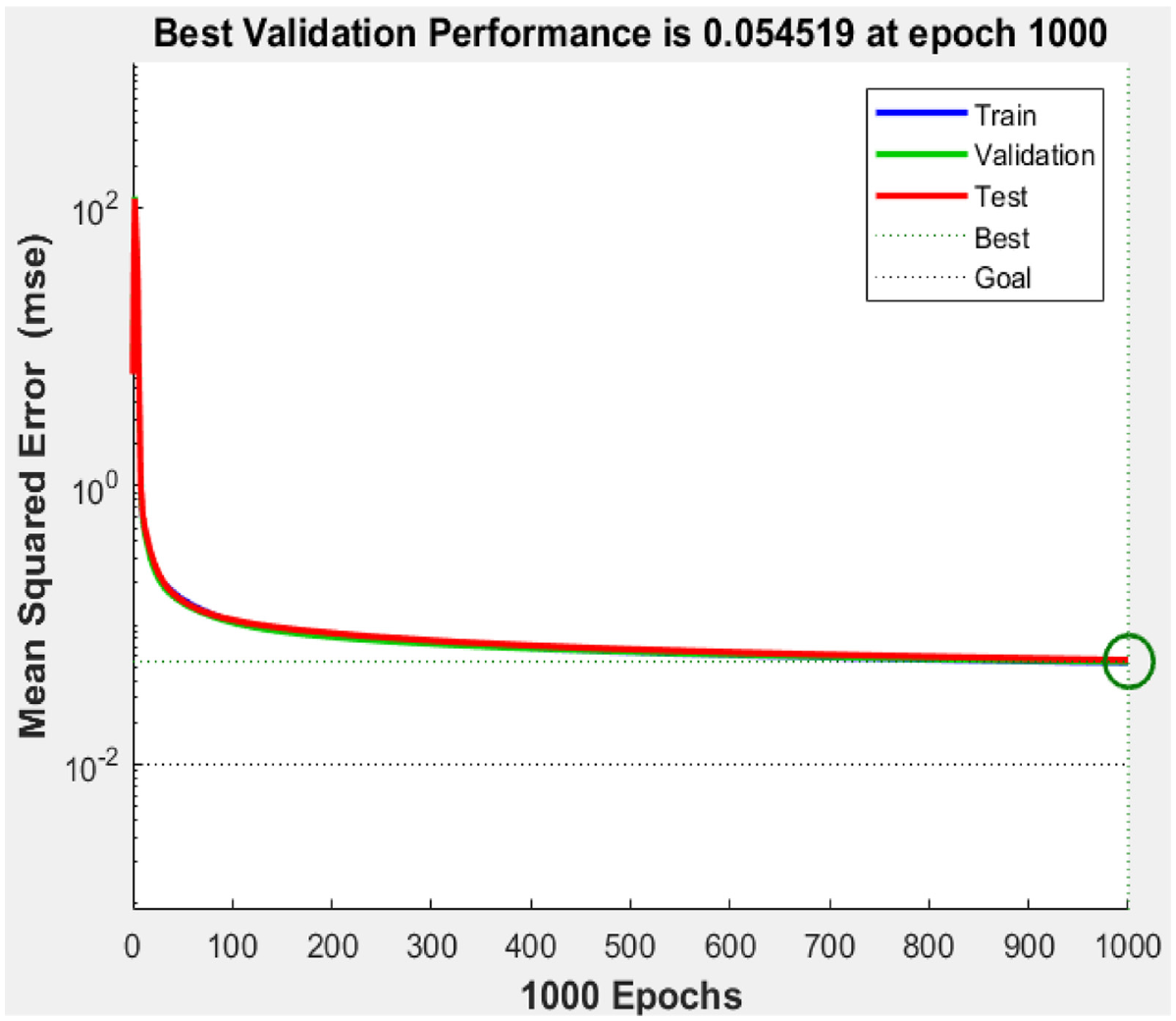
The performance graph obtained by the GD algorithm.

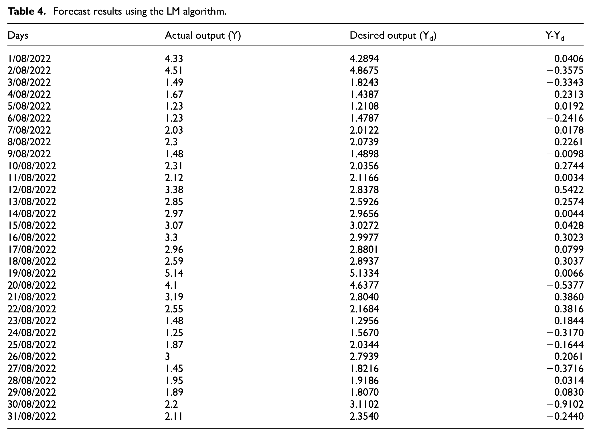
The errors obtained by both algorithms demonstrate that the program is well-trained, which justifies the accurate estimations of the wind speed for August as shown in Tables 4 and 6 and illustrated in Figures 11 and 12. These results demonstrate that the LM algorithm is more effective than GD algorithm for our site.

Table 4.

Forecast results using the LM algorithm.

Days	Actual output (Y)	Desired output (Y_d)	Y-Y_d
1/08/2022	4.33	4.2894	0.0406
2/08/2022	4.51	4.8675	−0.3575
3/08/2022	1.49	1.8243	−0.3343
4/08/2022	1.67	1.4387	0.2313
5/08/2022	1.23	1.2108	0.0192
6/08/2022	1.23	1.4787	−0.2416
7/08/2022	2.03	2.0122	0.0178
8/08/2022	2.3	2.0739	0.2261
9/08/2022	1.48	1.4898	−0.0098
10/08/2022	2.31	2.0356	0.2744
11/08/2022	2.12	2.1166	0.0034
12/08/2022	3.38	2.8378	0.5422
13/08/2022	2.85	2.5926	0.2574
14/08/2022	2.97	2.9656	0.0044
15/08/2022	3.07	3.0272	0.0428
16/08/2022	3.3	2.9977	0.3023
17/08/2022	2.96	2.8801	0.0799
18/08/2022	2.59	2.8937	0.3037
19/08/2022	5.14	5.1334	0.0066
20/08/2022	4.1	4.6377	−0.5377
21/08/2022	3.19	2.8040	0.3860
22/08/2022	2.55	2.1684	0.3816
23/08/2022	1.48	1.2956	0.1844
24/08/2022	1.25	1.5670	−0.3170
25/08/2022	1.87	2.0344	−0.1644
26/08/2022	3	2.7939	0.2061
27/08/2022	1.45	1.8216	−0.3716
28/08/2022	1.95	1.9186	0.0314
29/08/2022	1.89	1.8070	0.0830
30/08/2022	2.2	3.1102	−0.9102
31/08/2022	2.11	2.3540	−0.2440

Table 5.

Erreurs for The Tasting phase using LM.

MSE	0.0016
RMSE	0.0399
MAE	0.0040

Table 6.

Forecast results using the GD algorithm.

Days	Actual output (Y)	Desired output (Y_d)	Y-Y_d
1/08/2022	4.33	3.6414	0.6885
2/08/2022	4.51	4.3590	0.1509
3/08/2022	1.49	2.0429	−0.5529
4/08/2022	1.67	1.4150	0.2549
5/08/2022	1.23	1.1148	0.1151
6/08/2022	1.23	1.2851	−0.0551
7/08/2022	2.03	1.5498	0.4801
8/08/2022	2.3	1.8694	0.4305
9/08/2022	1.48	1.3068	0.1731
10/08/2022	2.31	1.6079	0.7020
11/08/2022	2.12	1.7856	0.3343
12/08/2022	3.38	2.6799	0.7000
13/08/2022	2.85	4.1446	−1.2946
14/08/2022	2.97	2.9753	−0.0053
15/08/2022	3.07	3.1785	−0.1085
16/08/2022	3.3	3.3565	−0.0565
17/08/2022	2.96	3.5030	−0.5430
18/08/2022	2.59	3.1970	−0.6070
19/08/2022	5.14	5.1555	−0.0155
20/08/2022	4.1	4.3150	−0.2150
21/08/2022	3.19	2.9294	0.2605
22/08/2022	2.55	2.4037	0.1462
23/08/2022	1.48	1.5562	−0.0762
24/08/2022	1.25	1.3914	−0.1414
25/08/2022	1.87	1.7704	0.0995
26/08/2022	3	2.7398	0.2601
27/08/2022	1.45	1.8574	−0.4074
28/08/2022	1.95	2.1466	−0.1966
29/08/2022	1.89	1.4495	0.4404
30/08/2022	2.2	2.2725	−0.0725
31/08/2022	2.11	1.8384	0.2715

Table 7.

Erreurs for The Tasting phase using GD.

MSE	0.0031
RMSE	0.0553
MAE	0.0055

Figure 11.

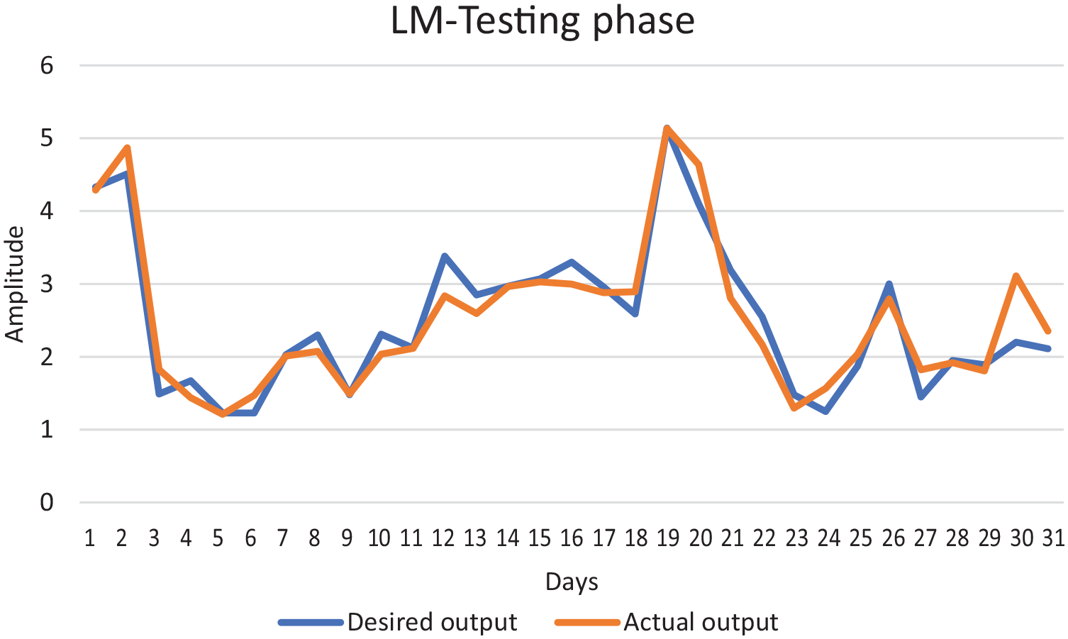
Wind speed prediction for August using the LM algorithm.

Figure 12.

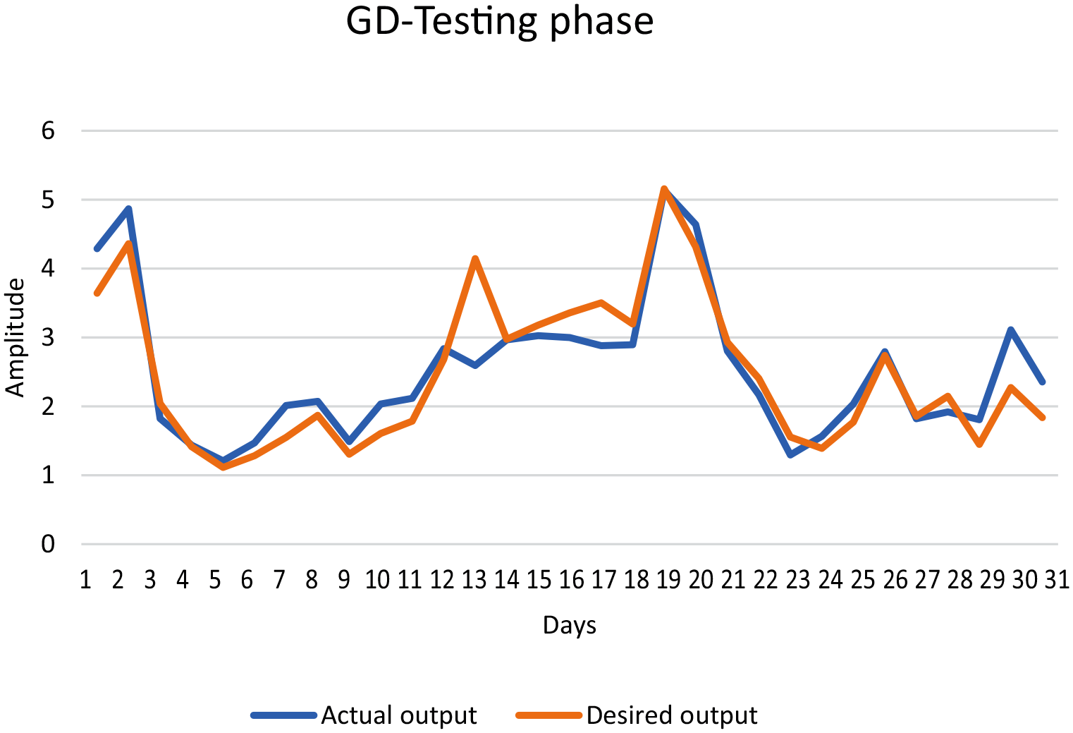
Wind speed prediction for August using the GD algorithm.

Training phase Testing phase

We need to test the program to judge the ability of the chosen model to predict the wind speed, for this purpose, we will apply the sim function to calculate the desired output (Ren et al., 2009)

T d = s i m (n e t, P t e s t)

(14)

Ptest: The test data of the neural network

Conclusion

The MLP study for Tetouan city, implemented by LM or GD in MATLAB to predict wind speed allowed us to conclude:

The application of MLP on dynamic features to identify and predict wind speed is feasible.

The MLP neural network has better fitting ability and higher predictive accuracy.

Despite the good results obtained by the two algorithms, the one of Levenberg Marquardt (LM) remains the most powerful, which gave a good accuracy with a coefficient MSE = 0.0458, compared to GD which has a value of MSE = 0.1101.

In a future article, we will study other predictive models to understand how they work and other algorithms designed to improve their performance.

Footnotes

Author contributions

All authors contributed to the study’s conception and design. Material preparation, data collection, and analysis were performed by [Wissal Masmoudi] and [Abdelouahed Djebli]. The first draft of the manuscript was written by [Wissal Masmoudi] and both authors commented on previous versions of the manuscript. Both authors read and approved the final manuscript.

Declaration of conflicting interests

The author(s) declared no potential conflicts of interest with respect to the research, authorship, and/or publication of this article.

Funding

The author(s) received no financial support for the research, authorship, and/or publication of this article.

Ethical approval

This study does not contain any studies with human or animal subjects performed by any of the authors.

ORCID iD

Wissal Masmoudi

References

Alboukadel (2020) Comment Normaliser et Standardiser les Données dans R pour une Visualisation en Heatmap Magnifique. In: Datanovia. Available at: https://www.datanovia.com/en/fr/blog/comment-normaliser-et-standardiser-les-donnees-dans-r-pour-une-visualisation-en-heatmap-magnifique/ (accessed 29 April 2023).

Amellas

Djebli

Echchelh

(2020a) Levenberg-Marquardt training function using on MLP, RNN and Elman Neural Network to optimize hourly forecasting in Tetouan City (Northern Morocco). Journal of Engineering Science and Technology Review 13(1): 67–71.

Amellas

El Bakkali

Djebil

, et al. (2020b) Short-term wind speed prediction based on MLP and NARX network models Keywords: Artificial neural network Daily prediction Multi-layer perceptron (MLP) NARX Recurrent neural network (RNN). Indonesian Journal of Electrical Engineering and Computer Science18: 150–157.

Analyze Shallow Neural Network Performance After Training - MATLAB & Simulink - MathWorks Benelux (n.d.) Available at: https://nl.mathworks.com/help/deeplearning/ug/analyze-neural-network-performance-after-training.html;jsessionid=d379fc28a97743b3080e4fd09b9d (accessed 29 April 2023).

Beauregard-Harvey

(2018) Amélioration des prévisions immédiates du vent et de la production éolienne. Epub ahead of print May 2018.

Nasr

(n.d.) Perceptron Multicouche Introduction à l’apprentissage automatique Master Sciences Cognitives Aix Marseille Université.

Qu’est-ce qu’un réseau neuronal artificiel ? - IONOS (n.d) Available at: https://www.ionos.fr/digitalguide/web-marketing/search-engine-marketing/quest-ce-quun-reseau-neuronal-artificiel/ (accessed 29 April 2023).

Ren

Liu

Rui

, et al. (2009) Application of Elman Neural Network and MATLAB to load forecasting. In: 2009 International conference on information technology and computer science, Kiev, July 2009, pp.55–59, New York, NY: IEEE. Available at: https://ieeexplore.ieee.org/document/5190016/ (accessed 5 May 2023).

Salami

Ajavon

Kodjo

, et al. (2017) Prédiction de la moyenne horaire de la vitesse du vent sur le site de Lomé par réseau de neurones. Epub ahead of print 2017.